SalaciaML-2-Arctic — a deep learning quality control algorithm for Arctic Ocean temperature and salinity data

We have extended a classical quality control (QC) algorithm by integrating a deep learning neural network, resulting in SalaciaML-2-Arctic, a tool for automated QC of Arctic Ocean temperature and salinity profile data. The neural network component was trained on the Unified Database for Arctic and Subarctic Hydrography (UDASH), which has been quality-controlled and labeled by expert oceanographers. SalaciaML-2-Arctic successfully reproduces human expertise by correcting misclassifications made by the classical algorithm, reducing False Negatives (samples incorrectly classified as “bad”) by 96% for temperature and 99% for salinity. When used in combination with a visual post-QC by human experts, it achieves a workload reduction of approximately 60% for temperature and 85% for salinity. All code and data required to reproduce the analysis or apply the method to other datasets are openly available via PANGAEA and GitHub. Moreover, SalaciaML-2-Arctic is accessible as a browser-based application at https://mvre.autoqc.cloud.awi.de, enabling its use without software installation or programming knowledge.

1 Introduction

Climate change is in full swing with drastic consequences for humankind (Rockström et al., 2023) and the global oceans play a fundamental role by absorbing more than 90% of the anthropogenic heat in the Earth system Li et al. (2023). The Arctic region is one of the most susceptible places on earth revealing dramatic changes also known as Arctic amplification (Rantanen et al., 2022). These environmental changes have been observed by measuring the state of the Arctic for decades with in situ instruments (Centurioni et al., 2019) and satellites (Wei et al., 2022) as well as using models (Xu and Li, 2023) to predict the evolution of the complex system. The detection of change has to rely on baseline measurements, in environmental science, provided in the form of climatologies. Hence the availability and creation of climatologies is crucial to identify and monitor changes. Behrendt et al. (2018, hereafter B2018) compiled a comprehensive hydrographic database (UDASH, Unified Database for Arctic and Subarctic Hydrography) of the northern high latitudes, which can be used for diverse applications such as studies of the ocean state and circulation, model validation and climate indicators (e.g. Lyu et al., 2022; Rabe et al., 2022; Sumata et al., 2018, and more). These hydrographic observations of temperature and salinity are Essential Ocean Variables (EOV) and Essential Climate Variables (ECV), as defined by the Global Ocean Observing System and Global Climate Observing System (GOOS, 2025; GCOS, 2025). A crucial aspect in the creation of baseline datasets is the quality of the data, which should be as good as possible. Data for the UDASH dataset have been retrieved from more than 20 data centers/sources, which follow different quality control procedures and different standards. Hence the challenge of B2018 was to bring the data from diverse sources onto a common quality level by adapting the best quality control algorithms from existing literature and applying them to the data. This involves detecting duplicates, outliers, spikes, suspect gradients, density inversions and more. However, the aim to create a well cleaned dataset in addition to the complex nature and large heterogeneity and diverse variability of the data, caused the algorithmic quality checks being too sensitive, i.e. too many “good” data were classified “bad”. Removing too many “good” data is a crucial problem in many ways, (i) we loose important information on environmental impact, (ii) we loose variability and (iii) we loose time and money, i.e. every sample has a monetary value. As a consequence B2018 applied an extensive visual/manual quality control by visualizing thousands of ocean profiles and correcting misclassifications, mostly by changing the sample classification from “bad” to “good”. Thus, UDASH is an Arctic baseline dataset that sets a benchmark in terms of quality and has the potential in contributing to a new Arctic climatology.

Quality control of ocean measurements is an important topic worldwide. The authors of this paper are members of the organization International Quality-controlled Ocean Database (IQuOD Domingues et al., 2018), that aims at developing a global ocean dataset as a baseline in terms of data consistency and QC. Further, we are involved since many years in the EU SeaDataNet infrastructure (Simoncelli et al., 2018) and EMODnet Chemistry (Lipizer et al., 2023), which compile and quality control ocean data from more than 100 data centers in Europe using sophisticated QC schemes. Although many powerful algorithms exist to identify errors in ocean data (Good et al., 2023; Tan et al., 2023), still the best results are obtained by human ocean expert visual QC. Visual QC is a time demanding effort and algorithmical help is already heavily used. However, existing methods still leave much room for improvement. Artificial intelligence (AI) has the potential to overcome current limitations (Mieruch et al., 2021) by using available large human visually QC’ed datasets. Many other approaches are investigated, e.g. Zhang et al. (2023) used an unsupervised classification QC of Argo float data using a Gaussian mixture model. Xie et al. (2023) used an LSTM (Long short-Term Memory) model to detect outliers in ocean data (unsupervised). QC is an important topic also in other fields, Bandaru et al. (2024) developed a deep learning LSTM for the QC of soil moisture, and Schulz et al. (2025) review very thoroughly the current state-of-the-art of ML for sensor QC. Making use of new and powerful AI programming frameworks and suitable strong computer hardware and large datasets, ML applications on data QC are investigated heavily. Many promising works already exist, however, the future will show if these new tools enter the operational field and support current procedures. Our contribution to this endeavor is the development of an AI algorithm, trained on human expert knowledge to support ocean experts in the time consuming task of ocean data QC. This work outlines the available data and quality control algorithms in Section 2, describes our AI approach and the implementation in Section 3. The results are shown in Section 4. The online service of our tool is presented in Section 5. We conclude with a summary, brief discussion and an outlook in Section 6.

2 Data and quality control

UDASH contains a large and comprehensive number of publicly available ocean data for the time period 1980-2015, north of 65° N. In total UDASH includes 288.532 oceanographic profiles measured mainly with conductivity–temperature–depth (CTD) probes, bottle samples analyzed in the laboratory, mechanical thermographs and expendable thermographs. The crucial point is that the approximately million single observations of in situ temperature and practical salinity (hereafter referred to as “salinity”) have been thoroughly quality controlled based heavily on the works of Gronell and Wijffels (2008). The original dataset can be retrieved from

• https://doi.pangaea.de/10.1594/PANGAEA.872931 (Behrendt et al., 2017).

For our analysis we have created two datasets, one for temperature and one for salinity available at

• https://doi.pangaea.de/10.1594/PANGAEA.983690 (Kreps and Mieruch, 2025).

These datasets can be used to fully reproduce our analysis.

The original quality checks comprise the following tests, which are only roughly explained here, for exact procedures we refer to B2018 and the citations therein.

● Duplicate checks:

○ CTD-sensor data are preferred over water samples analyzed in the laboratory if both are measured at the same time.

○ In the case of “near” duplicates, the profiles with the most data are retained.

● Position checks:

○ Data located over land are excluded.

○ Data from “chaotic” ship tracks, containing unrealistic jumps of the position, are excluded.

● Outlier:

○ Temperatures outside −2 and 15°C and

○ Salinity outside 10 and 38 (depth < 30m) and 25 and 38 (depth ≥30m) are marked “bad”.

● Spikes:

○ Upper 100 m: abs(temperature gradients) ≥0.5°C/m and abs(salinity gradients) ≥0.5m⁻¹ are marked “bad”.

○ Deeper waters: a Hampel identifier has been used, i.e. a sliding window along the profiles, median and standard deviations are calculated to identify and mark outliers; details in B2018.

● Suspect gradients:

○ The depth-by-temperature gradient has been calculated inspired by Gronell and Wijffels (2008), but thresholds have been adopted:

○ Upper 100 m: Gradients between −0.1 and 1m/°C considered “bad”.

○ Deeper waters: Gradients between −0.25 and 5m/°C considered “bad”.

○ For salinity, the salinity-by-depth gradient has been used with the following thresholds:

○ Upper 100 m: Gradients larger 2m⁻¹ considered “bad”.

○ Below 100 m and above 500 m: Gradients larger 1m⁻¹ considered “bad”.

○ Deeper waters: Gradients larger 0.1m⁻¹ considered “bad”.

● Density inversion:

○ Upper 100 m: Gradients smaller −0.08kgm⁻⁴ considered “bad”.

○ Deeper waters: Gradients smaller −0.03kgm⁻⁴ considered “bad”.

● Statistical screening:

○ Different statistical parameters of a profile are compared to surrounding profiles; details in B2018.

B2018 used a procedure that classifies every sample that has been detected by a check with a quality flag, e.g. “2” for the suspect gradient and “4” for the spikes. The thresholds for the tests have been derived empirically based on UDASH subsets that have been fully visually checked. It is reasonable that such hard thresholds will never separate the different error classes exactly in a large dataset like UDASH. The tuning of the thresholds is a compromise of detecting nearly all “bad”, to create a clean dataset, which is desired, by not removing too many “good”. However, regarding the immense size of the dataset a full visual check is not feasible, due to the need for substantial human resources. Therefore, the only way forward is to tune the sensitivity of the thresholds in a way to detect most (nearly all) “bad”, accept the “good” and perform a post-QC only on the “bad” to identify the wrongly classified “bad”, which are actually “good”. Therefore, in this approach we cannot identify False Positives, i.e. wrongly flagged “good” samples. Nevertheless, according to our tests on smaller UDASH subsets, the number of False Positives is very small and acceptable, because of the high sensitivity of the automatic checks. The consequence, however, is that in a large dataset, many samples are flagged as “bad” even though they are actually “good”. If a lot of actually good data were classified as bad, extensive visual inspection of the profiles was previously required to manually verify and correct the classification if necessary.

In this study we develop a deep learning model to imitate the human expertise of correcting the misclassifications by the classic QC checks. The aim is to reduce the workload of the ocean experts. As a starting point we focus on the spikes and suspect gradients, which are similar types of errors (mathematically). For the Statistical screening errors, we are planning to investigate other neural network architectures in the future.

3 Methods

3.1 Concept of artificial intelligence in quality control of ocean data

As explained above, a large number of profiles underwent visual inspection. Specifically, all profiles flagged by the automated checks were examined manually by B2018. During these checks B2018 decided to accept or reject the samples detected as “bad”. Therefore, the result of the visual QC performed by B2018 is that some data samples automatically detected as “bad” were set back to “good” after visual inspection. The final UDASH dataset therefore contains a mixture of “good” and “bad” flagged samples, which are defined on the one hand by strict rules and thresholds, i.e. the classic automatic checks. On the other hand the quality flags are changed by experts during the visual QC. From an algorithmical point of view the dataset therefore contains some “QC ambiguities”. For instance a depth-temperature gradient at 40m depth of size 0.9m/°C would be considered “bad” by the suspect gradient check. However, the following visual QC by the experts could have returned the quality flag of that sample back to “good” (flag 0). The reasons to change a flag from “bad” to “good” are diverse and best explained with expert knowledge. They comprise additional visual checks of that profile against surrounding profiles, knowledge and experience with data from specific regions, depths and seasons, oceanographic knowledge about water dynamics, currents, fronts, sea ridges and many more. The visual QC is therefore complex and it cannot be formulated in the frame of classical algorithms, such as the quality checks above. Here, artificial intelligence provides a suitable instrument, because it is able to “learn” such complex patterns and can mimic human behavior. The challenge is to develop and train an AI algorithm to “learn” human QC or oceanographic expert knowledge, of course without understanding the reasoning.

3.2 The approach of an AI algorithm for ocean temperature and salinity QC

Our approach is based on the works conducted in Mieruch et al. (2021), who developed the SalaciaML algorithm for the Mediterranean Sea, which was probably one of the first attempts to train neural networks on ocean QC. The results in Mieruch et al. (2021) were promising and the algorithm “learned” skilfully to classify “good” and “bad” data. However from a practical point of view SalaciaML was still too sensitive and removed/flagged too many data with good quality. Nevertheless the choice of using a MLP (Multilayer Perceptron) architecture was suitable. We performed a comparative analysis using UDASH data, employing a variety of machine learning algorithms for benchmarking. These included decision trees, k-means clustering, Support Vector Machines (SVM) with various kernels (Linear, RBF, Polynomial with optimized degrees, and Sigmoid), Random Forests with an optimized tree count, K-nearest neighbors with an optimized K value, Linear Discriminant Analysis (LDA), and Naive Bayes. In addition, we utilized deep learning through Convolutional Neural Networks (CNN), where profile segments were represented as matrices and the output reflected the quality flags for each sample within these segments. Among all the methods tested, the Multilayer Perceptron (MLP) demonstrated the highest performance. However, a problem of the MLP is that it is very sensitive, i.e. it detects too many actually “good” data as “bad”. The solution to this problem turned out to be a constraint. Luckily the UDASH data provides such a constraint by design. Our aim is to imitate the human expert not the classical algorithmic checks. We had to apply the MLP only to the samples that have been already flagged “bad” by the classic algorithmic checks. Therefore, the only task of the MLP (the AI) of SalaciaML-2-Arctic is to check and maybe turn the flag - “bad” into the flag “good”, like the human expert. This approach is very different to the one in (Mieruch et al., 2021), where SalaciaML was used to detect “bad” data. With the AI part of SalaciaML-2-Arctic we detect “good” data among the seemingly “bad”, i.e. we correct misclassifications. Thus, SalaciaML-2-Arctic is actually a two-step hybrid model, with a first classical step (the QC checks) and a following AI (MLP) step, which imitates the human expert decision to reduce the final workload for the experts.

3.3 Technical implementation

In the following we describe the technical implementation mostly from a conceptual point of view. However, readers who are not interested in these technical details may skip this section. Those who want to dive deeper into it are recommended to investigate the source code provided at https://github.com/GastonKreps/SalaciaML-2-Arctic (GastonKreps and smieruch, 2025).

● Step 1: From the original UDASH, we removed all samples, which have a missing temperature value (-999).

● Step 2: We implemented the spike and suspect gradient checks in Python to create the classical flags, without human intervention, which are not included in the original UDASH dataset. These classically created flags form our “baseline-model”, against which we evaluate the hybrid classical + MLP model.

● Step 4: Now we constrain the development of the MLP to only “bad” samples that have been detected by our “baseline-model”. Thus, we ignore all “good” samples. Again, what we want is that the MLP “learns” to turn back “bad” flags to “good”, similar to the manual/visual procedure by ocean experts. In a few cases the classical algorithms detected unusual many suspect gradients in a profile, which hampered the training. Therefore we filtered out all profiles with more than 20 flags and leave them for a visual inspection.

● Step 5: The design, training and evaluation with Python Keras (Chollet et al., 2015) and Scikit-learn:

1. Features:

● Year

● Month

● Longitude

● Latitude

● Depth

● Temperature/Salinity

● Gradients

2. Based on several tests we decided to use a fully connected, relative narrow MLP with 4 hidden layers with 64 x 32 x 16 x 8 nodes.

3. We split the flagged as “bad” samples of the profiles randomly into 70% training, 25% validation and 5% testing data. It is important to note that we do not split the profiles themselves to avoid having samples from the same profile in the training data and the test data.

4. For the training we used a “batch size” of 16.384 with the Adam optimizer and binary cross-entropy as the loss function.

5. The dataset to train, validate and test the MLP contains only the flagged as “bad” samples identified by the classical checks, among which are a certain number of wrong classification, which should actually be flagged as “good”. To address the class imbalance in the dataset, we employed the classweight parameter and the ROC (Receiver Operating Characteristic) curve for optimal threshold tuning. The classweight parameter adjusts the weight of each class based on the distribution in the training dataset, ensuring that the minority class is not overlooked during training (Johnson and Khoshgoftaar, 2019). The ROC curve, used with the validation dataset, helped in fine-tuning the classification threshold to achieve a balance between sensitivity and specificity (Mieruch et al., 2021).

4 Results

The results of the classical auto QC and the SalaciaML-2-Arctic, the two step classical + AI system, are best explained by evaluating the loss curves, the confusion matrices, and the ROC curves for temperature and salinity. To fully reproduce our results and/or to use SalaciaML-2-Arctic in real world applications, we provide the algorithms at https://github.com/GastonKreps/SalaciaML-2-Arctic. In addition SalaciaML-2-Arctic can be applied easily to own data at our online app https://mvre.autoqc.cloud.awi.de.

4.1 Temperature

A crucial aspect in machine learning is the evaluation of the loss curve, which is generated during the model training and validation phases. Figure 1 shows the loss curve for the temperature QC. The loss curve represents a measure of the error between predicted classes and actual classes (“good” and “bad”), where we used the binary cross-entropy as loss function. The blue curve in Figure 1 represents the loss during the training – the decrease over the training epoches indicates that the model is indeed “learning”. The orange curve depicts the loss of the model applied during training to the validation dataset, which is not used for the training, hence unknown to the model. The orange curve follows very closely the blue curve, which indicates that the model is nearly as good on unknown data as on training data, which depicts the success of the training. At a certain point an increase is expected, happening when the model starts “learning” the noise pattern in the training set, which is different in the validation set, and thus cannot be predicted by the model. This is the optimal point to stop the training. Another important metric is the ROC curve, illustrated in Figure 2, which provides a graphical representation of the performance of the MLP. The curve plots the True Positive Rate (TPR) against the False Positive Rate (FPR) at various classification threshold settings, offering insights into the trade-off between the TPR and FPR. The objective optimal classification threshold is given by the most top-left point in the curve, which we use accordingly. Thus, the ROC handles the imbalance of the data as well as the confidence of the model by choosing a classification threshold different than 0.5, which would be used in a case of class balance. Here, for temperature, the best threshold is observed at 0.37. Finally we show the confusion matrices for the classical algorithm and the SalaciaML-2-Arctic (MLP part), both applied to the test dataset, i.e. only “bad” classifications by the classical checks.

Figure 1

Figure 1. Loss curve generated during the temperature training and validation phase. The blue curve shows the loss for the training dataset, the orange curve depicts the loss for the validation dataset.

Figure 2

Figure 2. ROC curve for the SalaciaML-2-Arctic system. The curve shows the performance of the validation dataset with the best threshold indicated.

● TP (true positive): The correctly classified “good” data.

● FP (false positive): The false classified “good” data (actually “bad”).

● FN (false negative): The false classified “bad” data (actually “good”).

● TN (true negative): The correctly classified “bad” data.

Since the test dataset only includes samples, which have been classified “bad” by the classic algorithms it is clear that the left confusion matrix (Figure 3) has only True Negatives and False Negatives. Hence the 1199 False Negatives are actually “good”, i.e. have been turned from “bad” to “good” by the human expert. The confusion matrix of the MLP, on the right, shows that the deep learning system is able to identify 96% of the False Negatives, which are actually “good”, resulting in 1151 True Positives. At the same time the MLP is able to keep 99% of the True Negatives, making only a very small error in turning “bad” to “good” wrongly, indicated by the 7 False Positives. Finally we show two example profiles in Figure 4.

Figure 3

Figure 3. Confusion matrices for temperature. Left: classic algorithms, right: MLP, both applied to the test dataset.

Figure 4

Figure 4. Examples, where the SalaciaML-2-Arctic turns seemingly “bad” flags back to “good”. Green circles indicate samples, which have been classified “bad” by the classical algorithms. Blue circles represent the final “bad” data after visual expert QC. Red circles depict the results of the SalaciaML-2-Arctic.

● Green Circles (Classical algorithm): These indicate the data points flagged as “bad” by the classical quality control algorithms.

● Blue Circles (Expert QC): The blue circles represent data points confirmed as “bad” after the visual inspection by human experts.

● Red Circles (SalaciaML-2-Arctic): These circles denote the results by the SalaciaML-2-Arctic model, i.e. keeping the classification as “bad”.

The left panel of Figure 4 shows a profile, where the classical check has identified two “bad” samples. The human expert however changed those back to “good” - we see no blue circle. Similar there is no red circle visible, indicating that the neural network changed the quality of that sample back to “good” as well. This is exactly the workload reduction, because in an operational setting using SalaciaML-2-Arctic, such a profile would have not been shown to the human expert, rather it would have been automatically accepted as “good”. Without the ML component a visual inspection of that profile would have been needed. The right panel of Figure 4 shows a profile, where the classic algorithm detects a “bad” sample, which is kept “bad” by the human expert (blue circle) and the MLP (red circle).

4.2 Salinity

Similar to the parameter temperature we show the results for salinity. Figure 5 represents the loss curve. Here we see again a steep learning progress during the first epochs and a smooth decrease until ca. 900 epochs, where the overfitting starts. Figure 6 depicts the ROC for salinity with an optimal classification threshold at 0.17. The respective confusion matrices are shown in Figure 7. Similar to temperature the left confusion matrix for the classical algorithms (Figure 7) has only True Negatives and False Negatives. Hence the 2717 False Negatives are actually “good”, i.e. have been turned from “bad” to “good” by the human expert. The confusion matrix of the MLP, on the right, shows that the deep learning system is able to identify 99% of the False Negatives, which are actually “good”, resulting in 2678 True Positives. At the same time the MLP is able to keep 98% of the True Negatives, making only a very small error in turning “bad” to “good” wrongly, indicated by the 9 False Positives. Finally we show two example profiles in Figure 8. The left panel of Figure 8 shows again the workload reduction achieved by the neural network component, which would classify this profile as “good”, hence it would not have been shown to the human expert for visual control. The right panel of Figure 8 shows that truly “bad” samples are classified “bad” as well by the neural network.

Figure 5

Figure 5. Loss curve generated during the salinity training and validation phase. The blue curve shows the loss for the training dataset, the orange curve depicts the loss for the validation dataset.

Figure 6

Figure 6. ROC Curve for the SalaciaML-2-Arctic system. The curve shows the performance of the validation dataset with the best threshold indicated.

Figure 7

Figure 7. Confusion matrices for salinity. Left: classic algorithms, right: MLP, both applied to the test dataset.

Figure 8

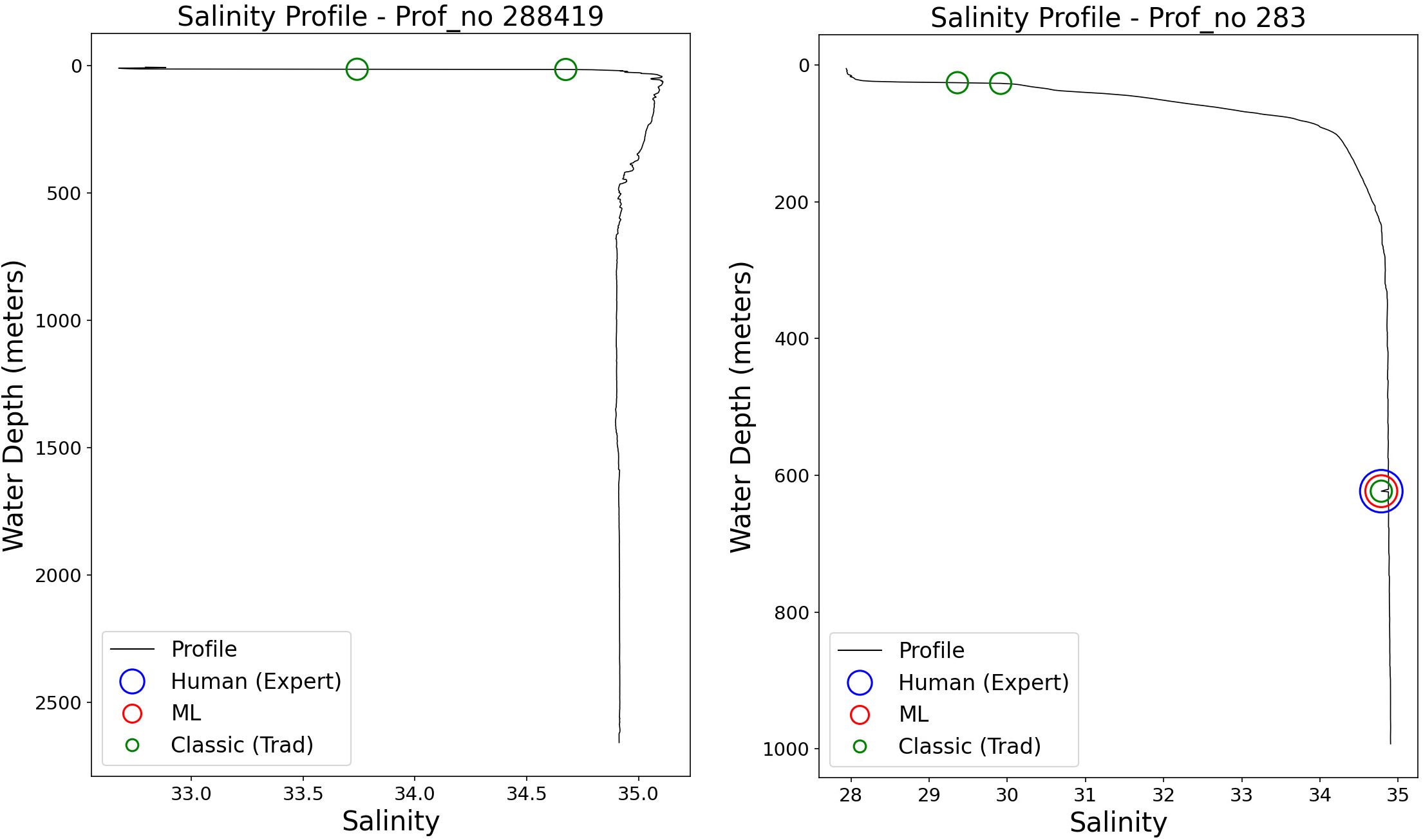
Figure 8. Examples, where the SalaciaML-2-Arctic turns seemingly “bad” flags back to “good”. Green circles indicate samples, which have been classified “bad” by the classical algorithms. Blue circles represent the final “bad” data after visual expert QC. Red circles depict the results of the SalaciaML-2-Arctic.

5 autoQC web app

We have created an online service for users to easily apply SalaciaML-2-Arctic in the browser, without installing any software on private computers. The app, which we name autoQC is available at https://mvre.autoqc.cloud.awi.de. Users have to login via the Helmholtz AAI, a single-sign-on system that provides access via research institutes as well as other systems e.g. ORCID, Google, GitHub. The user has to follow a simple three step procedure, i.e, uploading the data, processing and finally downloading the quality controlled data. At the moment the upload is limited to 50 MB (zipped). If users want to process larger datasets, we suggest to contact us, and we will find solutions. During the data upload the browser must not be closed. As soon as the data are uploaded, the processing starts in the background and users can logout or close the browser. We inform the user via email when the processing is finished. Further, the user has to decide to process either temperature data or salinity data. SalaciaML-2-Arctic adds two extra columns to the data, representing the quality information, i.e. the flags, thus we do not change or remove the original data. One extra column provides the classical flags, the other represents the final SalaciaML-2-Arctic flags. Details how to format the data are given in the dedicated documentation in the online app. The final output data can be downloaded as a simple .csv file.

6 Summary, discussion and outlook

We have developed an AI algorithm, which we name SalaciaML-2-Arctic, to support the QC of ocean temperature and salinity profile data. The tool is a hybrid model based on classic QC checks and a neural network that has been trained by human expert knowledge. The algorithm is available in Python and can be retrieved from our GitHub repository, and the UDASH data are available on the Pangaea website. In terms of FAIR data and algorithms, our work is fully reproducible. SalaciaML-2-Arctic improves existing classical QC procedures using AI. We recommend using SalaciaML-2-Arctic on Arctic temperature and salinity profile data to improve the quality. The SalaciaML-2-Arctic system has “learned” the QC procedure normally done by a human expert, who reevaluates QC’ed data from the classical checks and corrects misclassifications, i.e. data wrongly labeled “bad”. SalaciaML-2-Arctic “learned”, in a supervised setting, doing exactly what otherwise humans do, turning wrong “bad” flags back to “good”. The neural network is nearly as good as the human trainer and corrects 96% of wrong classifications for temperature and 99% for salinity. At the same time SalaciaML-2-Arctic generates nearly no errors, i.e. wrongly turning “bad” to “good”. Therefore we can say that SalaciaML-2-Arctic is a highly skilled system. In a scenario where ocean experts want to apply a post visual QC on the data, of course, all “bad” flagged data (by the MLP) must be inspected. For temperature, according to our test dataset, instead of inspecting 1950 samples, only 792 that are 40.6% have to be analyzed. For salinity only 15.8% of the samples have to be analyzed, i.e. instead of 3191 only 504. However, a small “price” has to be payed for using SalaciaML-2-Arctic, i.e. the few False Positives created by the MLP have to be accepted, because they are classified “good” and thus accepted. Applications can be diverse. If users have a very large dataset and no possibilities or resources for extra time consuming visual QC, SalaciaML-2-Arctic can be applied fully automated and results can be accepted, which provide a good compromise of removing (flagging) the truly erroneous data, but without making too many misclassifications as “bad”. If users have the capabilities and resources for a visual QC on the data, e.g. if it is a small dataset or if users want to create a high quality climatology, then SalaciaML-2-Arctic can be applied as a “first guess” and suggestions of our algorithm can be again inspected by experts and accepted or rejected. In this sense SalaciaML-2-Arctic gives hints to potentially “bad” data and supports experts in more efficiently locating problems in the data, which can be a real workload reduction and efficiency increase.

AI for supporting ocean data QC is still in it’s infancy. However, our results are promising. Ocean data QC is a global challenge and should be approached by international consortia, which is done by IQuOD, SeaDataNet, EMODnet and others. In this frame we will continue the development of the SalaciaML algorithms. The long-term goal is the expansion to global data, to other variables e.g. oxygen, carbon, nutrients, and to handle additional data checks. Therefore, high quality data is needed, QC experts must be included, and visualization and data experts as well as ML and AI specialists have to be involved. This would facilitate developing the future generation of ocean QC systems to support the high quality data product generation, science and decision making, improving the quality and consistency of the data, optimizing the final scientific research and knowledge extracted from the data.

Data availability statement

Publicly available datasets were analyzed in this study. This data can be found here: https://doi.pangaea.de/10.1594/PANGAEA.872931, https://doi.pangaea.de/10.1594/PANGAEA.983690; Code: doi: 10.5281/zenodo.16892415.

Author contributions

SM: Funding acquisition, Writing – review & editing, Software, Writing – original draft, Supervision, Investigation, Resources, Conceptualization, Project administration, Validation, Methodology, Data curation, Visualization, Formal Analysis. GK: Validation, Investigation, Software, Funding acquisition, Writing – review & editing, Visualization, Formal Analysis, Data curation, Methodology. MC: Validation, Visualization, Data curation, Methodology, Formal Analysis, Software, Investigation, Writing – review & editing, Conceptualization. FR: Writing – review & editing, Methodology, Software, Investigation. MV: Methodology, Data curation, Validation, Writing – review & editing. BR: Validation, Methodology, Data curation, Writing – review & editing. ST: Validation, Methodology, Writing – review & editing, Data curation. AB: Writing – review & editing, Validation, Data curation, Methodology.

Funding

The author(s) declare financial support was received for the research and/or publication of this article. This work is funded by the German Ministry of Research and Education (BMBF) under grant number 03F0888A, Mare:N – Küsten-, Meeres- und Polarforschung für Nachhaltigkeit. GK received funding from DataHub Earth and Environment of the Helmholtz Association and HIDA – the Helmholtz Information & Data Science Academy. BR and MV contributed to this work partly through the Changing Arctic Ocean (CAO) program, jointly funded by the United Kingdom Research and Innovation (UKRI) Natural Environment Research Council (NERC) and the BMBF, in particular, the CAO project Advective Pathways of nutrients and key Ecological substances in the ARctic (APEAR) grant number 03V01461.

Acknowledgments

This work would have been not possible without the support of many friends and colleagues. We thank Serdar Demirel for discussion on the first version of the SalaicaML algorithm. Many thanks go to Steffen Seitz for discussion on state-of-the-art machine learning techniques. Many thanks to Jay Ghosh for discussions during the 2024 AGU conference in Washington. We thank AWI's computing center in general and especially StefanPinkernell for great support with the GPU systems and David Kleinhans and Stephan Frickenhaus for project support. We are thankful for being part in the IQuOD community and for their great support.

Conflict of interest

The authors declare that the research was conducted in the absence of any commercial or financial relationships that could be construed as a potential conflict of interest.

Generative AI statement

The author(s) declare that no Generative AI was used in the creation of this manuscript.

Any alternative text (alt text) provided alongside figures in this article has been generated by Frontiers with the support of artificial intelligence and reasonable efforts have been made to ensure accuracy, including review by the authors wherever possible. If you identify any issues, please contact us.

Publisher’s note

All claims expressed in this article are solely those of the authors and do not necessarily represent those of their affiliated organizations, or those of the publisher, the editors and the reviewers. Any product that may be evaluated in this article, or claim that may be made by its manufacturer, is not guaranteed or endorsed by the publisher.

References

Bandaru L., Irigireddy B. C., PVNR K., and Davis B. (2024). Deepqc: A deep learning system for automatic quality control of in-situ soil moisture sensor time series data. Smart Agric. Technol. 8, 100514. doi: 10.1016/j.atech.2024.100514

Crossref Full Text | Google Scholar

Behrendt A., Sumata H., Rabe B., and Schauer U. (2017). A comprehensive, quality-controlled and up-to-date data set of temperature and salinity data for the Arctic Mediterranean Sea (Version 1.0). doi: 10.1594/PANGAEA.872931. Supplement to: Behrendt, A et al. (2017): UDASH -Unified Database for Arctic and Subarctic Hydrography. Earth System Science Data Discussions, 37 pp, doi: 10.5194/essd-2017-92

Crossref Full Text | Google Scholar

Behrendt A., Sumata H., Rabe B., and Schauer U. (2018). Udash – unified database for arctic and subarctic hydrography. Earth System Sci. Data 10, 1119–1138. doi: 10.5194/essd-10-1119-2018

Crossref Full Text | Google Scholar

Centurioni L. R., Turton J., Lumpkin R., Braasch L., Brassington G., Chao Y., et al. (2019). Global in situ observations of essential climate and ocean variables at the air–sea interface. Front. Mar. Sci. 6. doi: 10.3389/fmars.2019.00419

Crossref Full Text | Google Scholar

Chollet F., et al. (2015). Keras. Available online at: https://keras.io. (Accessed April 10, 2025).

Google Scholar

Domingues C., Palmer M., Gouretski V., Kizu S., Macdonald A., Boyer T., et al. (2018). A new world ocean temperature profile product (v0.1): the international quality controlled ocean database (iquod) 263–264.

Google Scholar

GastonKreps and smieruch. (2025). Gastonkreps/salaciaml-2-arctic: Salaciasalaciaml-2-arctic: Unified database for arctic and subarctic hydrography. doi: 10.5281/zenodo.16892415

Crossref Full Text | Google Scholar

GCOS (2025).Essential climate variables. Available online at: https://gcos.wmo.int/site/global-climate-observing-system-gcos/essential-climate-variables/ (Accessed June 6 2025).

Google Scholar

Good S., Mills B., Boyer T., Bringas F., Castelão G., Cowley R., et al. (2023). Benchmarking of automatic quality control checks for ocean temperature profiles and recommendations for optimal sets. Front. Mar. Sci. 9. doi: 10.3389/fmars.2022.1075510

Crossref Full Text | Google Scholar

GOOS (2025).Essential ocean variables. Available online at: https://goosocean.org/what-we-do/framework/essential-ocean-variables/ (Accessed June 6, 2025).

Google Scholar

Gronell A. and Wijffels S. E. (2008). A semiautomated approach for quality controlling large historical ocean temperature archives. J. Atmospheric Oceanic Technol. 25, 990–1003. doi: 10.1175/jtecho539.1

Crossref Full Text | Google Scholar

Johnson J. M. and Khoshgoftaar T. M. (2019). Survey on deep learning with class imbalance. J. Big Data 6, 27. doi: 10.1186/s40537-019-0192-5

Crossref Full Text | Google Scholar

Kreps G. and Mieruch S. (2025). UDASH-SalaciaML-2-Arctic: Unified Database for Arctic and Subarctic Hydrography - Simplified and extended for quality control analyses. doi: 10.1594/PANGAEA.983690

Crossref Full Text | Google Scholar

Li Z., England M., and Groeskamp S. (2023). Recent acceleration in global ocean heat accumulation by mode and intermediate waters. Nat. Commun. 14, 6888. doi: 10.1038/s41467-023-42468-z

PubMed Abstract | Crossref Full Text | Google Scholar

Lipizer M., Molina Jack M. E., Wesslander K., Fyrberg L., Tsompanou M., Iona A., et al. (2023). 2023 EMODnet Chemistry Regional sea eutrophication data collection and Quality Control loop. Tech. Rep. 1. doi: 10.13120/8XM0-5M67. OGS (Istituto Nazionale di Oceanografia e di Geofisica Sperimentale).

Crossref Full Text | Google Scholar

Lyu G., Serra N., Zhou M., and Stammer D. (2022). Arctic sea level variability from high-resolution model simulations and implications for the arctic observing system. Ocean Sci. 18, 51–66. doi: 10.5194/os-18-51-2022

Crossref Full Text | Google Scholar

Mieruch S., Demirel S., Simoncelli S., Schlitzer R., and Seitz S. (2021). Salaciaml: A deep learning approach for supporting ocean data quality control. Front. Mar. Sci. 8. doi: 10.3389/fmars.2021.611742

Crossref Full Text | Google Scholar

Rabe B., Heuzé C., Regnery J., Aksenov Y., Allerholt J., Athanase M., et al. (2022). Overview of the MOSAiC expedition: Physical oceanography. Elementa: Sci. Anthropocene 10, 62. doi: 10.1525/elementa.2021.00062

Crossref Full Text | Google Scholar

Rantanen M., Karpechko A. Y., Lipponen A., Nordling K., Hyvärinen O., Ruosteenoja K., et al. (2022). The arctic has warmed nearly four times faster than the globe since 1979. Commun. Earth Environ. 3. doi: 10.1038/s43247-022-00498-3

Crossref Full Text | Google Scholar

Rockström J., Gupta J., Qin D., Lade S. J., Abrams J. F., Andersen L. S., et al. (2023). Safe and just earth system boundaries. Nature 619, 102–111. doi: 10.1038/s41586-023-06083-8

PubMed Abstract | Crossref Full Text | Google Scholar

Schulz K., Niemann A., and Mietzel T. (2025). A review on how machine learning can be beneficial for sensor data quality control and imputation in water resources management. J. Hydroinformatics, jh2025017. doi: 10.2166/hydro.2025.017

Crossref Full Text | Google Scholar

Simoncelli S., Coatanoan C., and Myroshnychenko V. (2018). Seadatacloud temperature and salinity historical data collection for the mediterranean sea (version 1). product information document (pidoc), technical report, june 2018. doi: 10.13155/57036

Crossref Full Text | Google Scholar

Sumata H., Kauker F., Karcher M., Rabe B., Timmermans M.-L., Behrendt A., et al. (2018). Decorrelation scales for arctic ocean hydrography – part i: Amerasian basin. Ocean Sci. 14, 161–185. doi: 10.5194/os-14-161-2018

Crossref Full Text | Google Scholar

Tan Z., Cheng L., Gouretski V., Zhang B., Wang Y., Li F., et al. (2023). A new automatic quality control system for ocean profile observations and impact on ocean warming estimate. Deep Sea Res. Part I: Oceanographic Res. Papers 194, 103961. doi: 10.1016/j.dsr.2022.103961

Crossref Full Text | Google Scholar

Wei J., Hang R., and Luo J.-J. (2022). Prediction of pan-arctic sea ice using attention-based lstm neural networks. Front. Mar. Sci. 9. doi: 10.3389/fmars.2022.860403

Crossref Full Text | Google Scholar

Xie J., Jiang H., Song W., and Yang J. (2023). A novel quality control method of time-series ocean wave observation data combining deep-learning prediction and statistical analysis. J. Sea Res. 195, 102439. doi: 10.1016/j.seares.2023.102439

Crossref Full Text | Google Scholar

Xu M. and Li J. (2023). Assessment of sea ice thickness simulations in the cmip6 models with cice components. Front. Mar. Sci. 10. doi: 10.3389/fmars.2023.1223772

Crossref Full Text | Google Scholar

Zhang Q., Qian C., and Dong C. (2023). A machine learning approach to quality-control argo temperature data. Atmospheric Oceanic Sci. Lett. 16, 100292. doi: 10.1016/j.aosl.2022.100292. Special Issue: Machine Learning Applications for Atmospheric and Oceanic Sciences.

Crossref Full Text | Google Scholar