Abstract
To address the limitations in identifying complex anomaly patterns and the heavy reliance on manual labeling in traditional oceanographic data quality control (QC) processes, this study proposes an intelligent QC method that integrates Gated Recurrent Units (GRU) with a Mean Teacher–based semi-supervised learning framework. Unlike conventional deep learning approaches that require large amounts of high-quality labeled data, our model adopts an innovative training strategy that combines a small set of labeled samples with a large volume of unlabeled data. Leveraging consistency regularization and a teacher–student network architecture, the model effectively enhances its ability to learn anomalous features from unlabeled observations. The input incorporates multiple sources of information, including temperature, salinity, vertical gradients, depth one-hot encodings, and seasonal encodings. A bidirectional GRU combined with an attention mechanism enables precise extraction of profile structure features and accurate identification of anomalous observations. Validation on real-world profile datasets from the Bailong (BL01) moored buoy and Argo floats demonstrates that the proposed model achieves outstanding performance in detecting temperature and salinity anomalies, with ROC-AUC scores of 0.966 and 0.940, and precision–recall AUCs of 0.952 and 0.916, respectively. Manual verification shows over 90% consistency, indicating high sensitivity and robust generalization capability under challenging scenarios such as weak anomalies and structural profile shifts. Compared to existing fully supervised models, the proposed semi-supervised QC framework exhibits superior practical value in terms of labeling efficiency, anomaly modeling capacity, and cross-platform adaptability.
1 Introduction
Ocean buoys, as key observational platforms, play a vital role in the global ocean monitoring network. These buoys continuously record various physical and chemical parameters from the sea such as temperature, salinity, currents, atmospheric pressure, and wind fields, providing essential scientific support for climate change monitoring, marine ecosystem studies, and ocean disaster early warning systems (Kolukula and Murty, 2025). However, due to the long-term deployment in dynamic and complex marine environments, buoy data are susceptible to anomalies caused by sensor drift (Kent et al., 2019), extreme weather, and equipment aging (Zhu and Yoo, 2016). Therefore, rigorous quality control (QC) procedures are critical to ensure the reliability and usability of buoy observations.
In recent years, for the purpose of tackling the observation characteristics and data properties of various types of ocean buoys, various QC techniques have been developed to enhance the stability of data quality as well as its practical value. Traditional ocean data quality control (QC) methods typically include consistency checks, range tests, and distribution fitting to ensure the temporal, spatial, and physical coherence of the observations (Wen, 2014). In practice, several studies have proposed systematic QC procedures for surface buoy data. For example, Lei et al. (2022) developed a streamlined QC workflow consisting of preprocessing, statistical screening, local feature recognition, error control, and manual inspection. By introducing error tolerance mechanisms, their method effectively avoids excessive data rejection and significantly improves data integrity and representativeness. In addition, for specific parameters such as wave data, Liu et al. (2016) constructed a composite QC framework combining Grubbs’ test and local outlier detection, enabling the preservation of true anomaly events while enhancing sensitivity and adaptability. For moored buoy observations, Li et al. (2019) proposed an automated QC method based on meteorological and hydrological principles, incorporating range checks, extreme value detection, and correlation analysis. For Argo profiling floats, historical profile matching has been widely adopted for anomaly detection and correction—this involves comparing real-time data with statistical features from historical databases to ensure physical and statistical consistency (Wang et al., 2012). Moreover, Argo data also employ a delayed-mode quality control (DMQC) system to correct long-term sensor drift in pressure and salinity measurements, with fine adjustments using the OWC algorithm (Core Argo Data Management Team, 2021).
However, these traditional methods largely rely on manual verification. As data volume and real-time demands increase, their low efficiency and high labor costs have become significant limitations. Consequently, some researchers have attempted to develop automated QC systems based on rule-based techniques such as temperature range checks, vertical gradient analysis, and profile shape recognition, aiming for real-time anomaly detection in buoy datasets (Zhang et al., 2024). Nevertheless, these approaches typically depend on static thresholds and empirical rules, which are insufficient to accommodate the diversity of oceanic environments (e.g., remote regions or ecologically anomalous zones). Furthermore, traditional QC methods heavily rely on historical data for reference, which may itself be contaminated by noise, regional biases, or sparse spatial-temporal coverage, ultimately affecting the accuracy and robustness of quality control.
In recent years, deep learning methods have emerged as promising tools in buoy data quality control due to their nonlinear modeling capabilities, significantly improving anomaly detection accuracy and adaptability. For example, Li et al. (2018) leveraged association rules and clustering to identify extreme meteorological events, building effective anomaly recognition models. Leahy et al. (2018) applied neural networks to classify and correct historical climate observations using multidimensional features such as time, depth, and data source, thereby improving overall data consistency. For Argo profile QC, Sugiura and Hosoda (2020) proposed a learning method based on profile curve shapes, replacing traditional rule-based detection with automatic anomaly identification.
Further developments include the integration of multi-source observational data with neural networks for real-time meteorological anomaly detection (Xu et al., 2021); the application of multilayer perceptrons (MLPs) and deep neural networks (DNNs) to sea temperature classification tasks, enhanced by synthetic minority oversampling and weighted loss functions (Liu et al., 2021); the use of the SalaciaML model for efficient temperature anomaly detection on large Mediterranean datasets (Mieruch et al., 2021); the design of BP network–based automated QC workflows to improve observation consistency (Huang et al., 2023); the construction of particle swarm–optimized BP neural networks for anomaly detection under high-humidity conditions (Wang et al., 2024); and algorithm evaluation for pH data quality control, where the addition of near-surface reference points was proposed to improve QC accuracy (Wimart-Rousseau et al., 2024).
Despite these advances, deep learning–based methods still face significant challenges in real-world applications. Although MLPs and signature-path models have reduced manual effort and improved automation in anomaly detection, their performance remains highly dependent on the availability of high-quality labeled data. In practice, buoy observation data often suffer from sparse labeling, uneven data quality, and class imbalance, which hinder the ability of supervised learning models to fully capture the distribution of anomalous features. Under complex and dynamic oceanic conditions, such models tend to exhibit poor generalization and stability, limiting their broader applicability and scalability.
To address the issues mentioned above, we proposed a novel semi-supervised quality control framework based on the Mean Teacher architecture combined with a GRU-Attention network. This framework was designed to tackle label scarcity, complex anomaly patterns, and the need for real-time application. Structurally, it employed a teacher–student dual-network architecture, where GRU (Gated Recurrent Unit) modules capture temporal dependencies, and attention mechanisms enhance focus on anomalous profile layers. By enforcing consistency regularization between the teacher and student models, the framework enables the student model to learn from large volumes of unlabeled buoy data and discover underlying anomaly patterns, even when labeled data are limited. This approach reduced reliance on human labeling while maintaining high anomaly detection accuracy. In practical applications, the model can be integrated into automated buoy QC workflows for real-time anomaly detection and label generation, thus improving operational efficiency and responsiveness.
2 Data
2.1 Bailong buoy data
The Bailong-01 (BL01) buoy is a key fixed-point ocean observation platform deployed in the southern equatorial Indian Ocean warm pool under the RAMA program (Research Moored Array for African–Asian–Australian Monsoon Analysis and Prediction). It is located offshore to the southwest of Sumatra (see Figure 1 for detailed location). This region lies within the core area of tropical monsoon circulation and is influenced by a combination of oceanic processes, including the Indonesian Throughflow, seamount topography, and tropical gyre modulation (Sprintall et al., 2009), making it an important window for studying monsoon systems, oceanic dynamics, and climate variability. BL01 is capable of long-term, all-weather automatic observations. Its upper section is equipped with various meteorological sensors to measure and record air temperature, relative humidity, atmospheric pressure, wind speed, and wind direction. The lower section hosts multilayer oceanographic instruments, primarily including conductivity–temperature–depth (CTD) sensors and acoustic Doppler current profilers (Aquadopp), which acquire seawater temperature, salinity, and velocity data across multiple depth layers (Ning et al., 2022). The observation depth extends from the sea surface down to 700 meters. This study focused on the 20–100 m depth range, where sensor deployment is relatively dense and both temperature and salinity are measured in real time. This configuration offers high temporal and spatial resolution, making it particularly suitable for quality control and anomaly detection studies (see Figure 2 for the structure of the BL01 buoy).
Figure 1
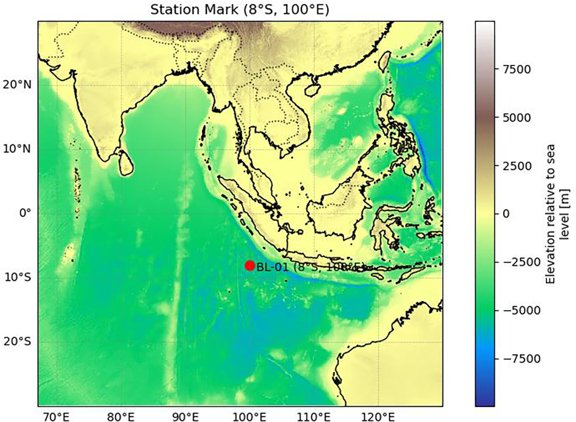
Location of the Bailong-01 (BL01) Buoy. (Bathymetric data source: GEBCO Compilation Group (2024), GEBCO 2024 Grid. DOI: 10.5285/1c44ce99-0a0d-5f4f-e063-7086abc0ea0f.).
Figure 2
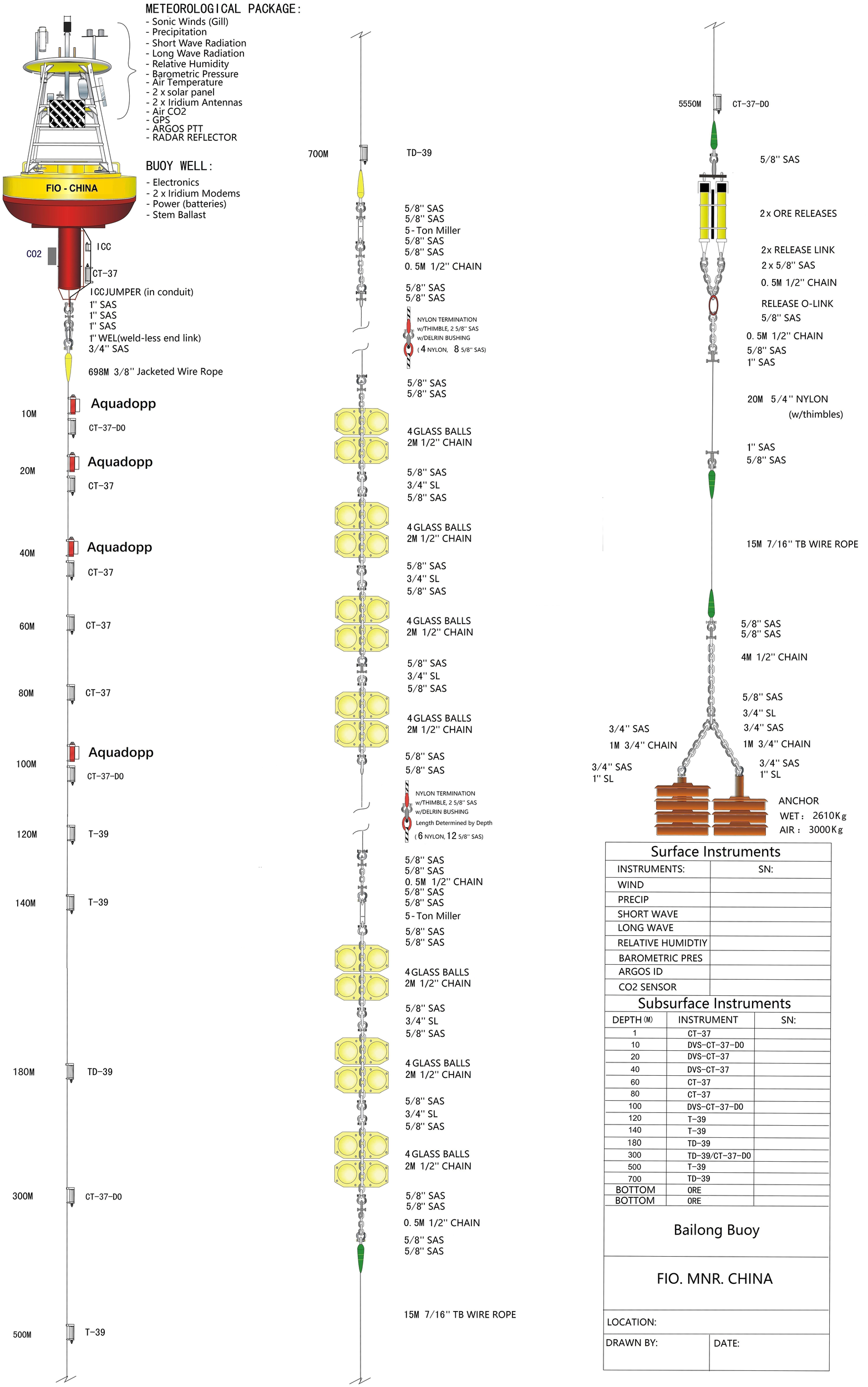
Structural diagram of the BL01 buoy.
The raw observational data used in this study were obtained from the profile sensors deployed during the 2014 and 2016 deployment cycles from the BL01 buoy. The data cover the period from 2014 to 2018 and were uniformly recorded in Standard Time. Measurement units follow international conventions: temperature is recorded in degrees Celsius (°C), salinity in practical salinity units (PSU), depth in meters (m), and pressure in decibars (dbar). The sampling interval is 10 minutes. The two datasets include the following parameter fields:
-
-Depth: Sensor depth (m)
-
-Pressure: Pressure at the observation point (dbar)
-
-Temperature: Seawater temperature (°C)
-
-Salinity: Salinity (PSU)
-
-Standard time: Recorded timestamp (Julian day format)
As shown in the statistical summary in Figure 3, the dataset from April 2014 to April 2015 contained a total of 259,348 records, while the dataset from October 2016 to January 2018 included 324,371 records, yielding a combined total of approximately 584,000 samples.It is important to note that the data used in this study were directly extracted by field technicians after buoy recovery and have not undergone any interpolation, smoothing, or quality control procedures. As a result, the dataset retains all anomalous signals from the original observation process, including disturbances, sensor drift, measurement errors, and pre-deployment test records.
Figure 3
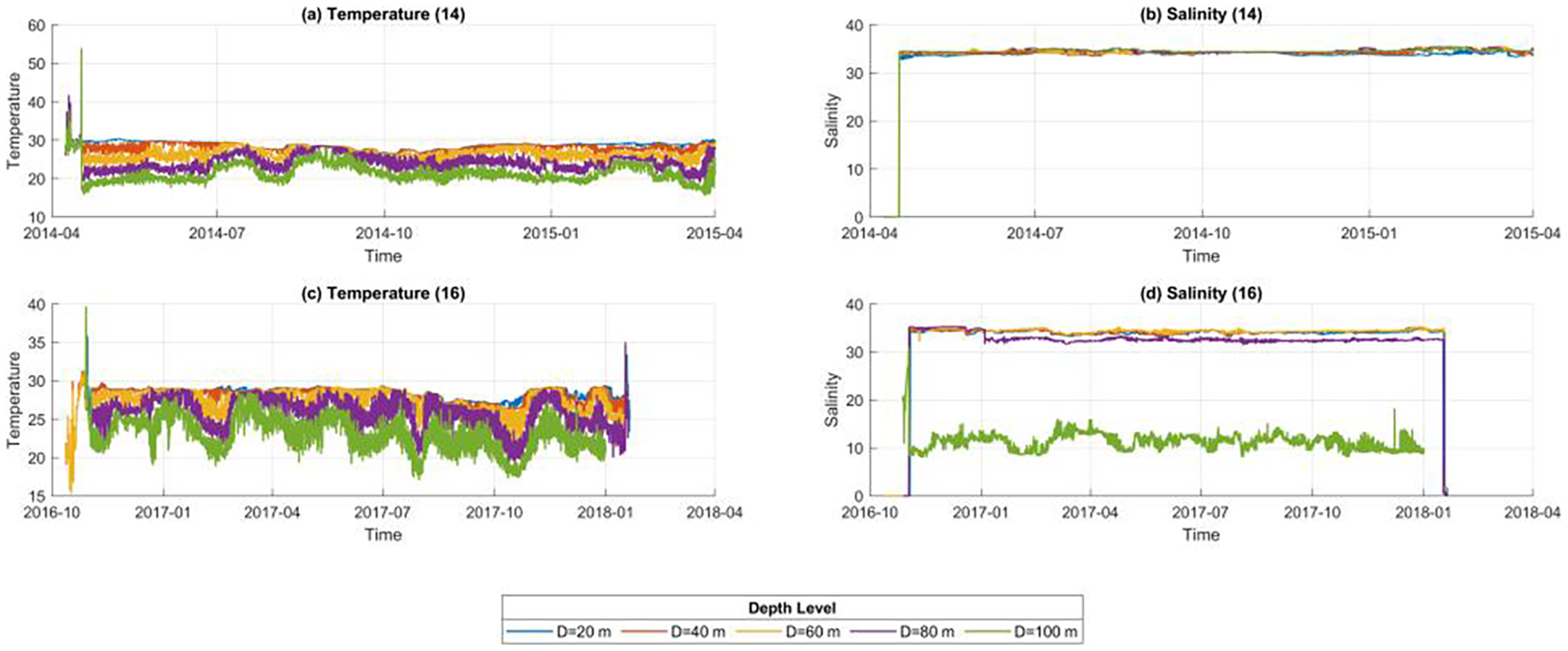
Distribution of BL01 buoy data [(a, b) Temperature and salinity data from 2014–2015; (c, d) Temperature and salinity data from 2016–2018].
2.2 Argo data
The dataset used in this study was obtained from the Argo float observations provided by the Integrated Marine Observing System (IMOS) of Australia. Specifically, four float IDs were selected: 5905211, 5905212, 5905213, and 5905214 (Hill et al., 2015). These floats are based on the NAVIS_EBR platform, manufactured by Sea-Bird Electronics (USA), and are equipped with standard conductivity–temperature–depth (CTD) sensor modules capable of real-time measurement of temperature (TEMP), salinity (PSAL), and pressure (PRES). The observational data are transmitted in real time via the IRIDIUM satellite network to the Commonwealth Scientific and Industrial Research Organisation (CSIRO) for data management and quality control (Wong et al., 2020).
The above floats were deployed sequentially in mid-November 2017 in the tropical region of the southeastern Indian Ocean, within a longitudinal range of 110.25°E to 119°E and a latitudinal band between 13.5°S and 14°S. The floats have remained in stable operational condition, and as of December 2024, each float had completed approximately 259 to 260 profiling cycles. For example, float 5905211 alone had produced approximately 256,921 raw observational records.
The dataset primarily included six core physical parameters: observation date, geographic coordinates (latitude and longitude), pressure (PRES), depth (DEPTH), temperature (TEMP), and salinity (PSAL). Each of these parameters was accompanied by a corresponding quality control (QC) flag—such as TEMP_QC, PSAL_QC, PRES_QC, DATE_QC, and POSITION_QC—to indicate potential data quality issues. For the TEMP and PSAL fields, every data point was tagged with a QC flag: a value of “1” denoted data that had passed QC procedures and was considered valid or high quality, while a value of “0” indicated data that failed QC or was considered anomalous.
After filtering all measurements with depths shallower than 130 m, a total of 110,454 valid records were retained across the four Argo floats. These data points were primarily distributed in the tropical southeastern Indian Ocean, centered around approximately 13.5°S and 119°E, a location geographically close to the Bailong buoy site. The time span of the Argo data begins in November 2017 and continues to the present, and as illustrated in Figure 4, the vertical distributions of temperature and salinity from the selected Argo profiles are clearly presented, providing an overview of their spatial and temporal coverage that complements the Bailong buoy observations.
Figure 4
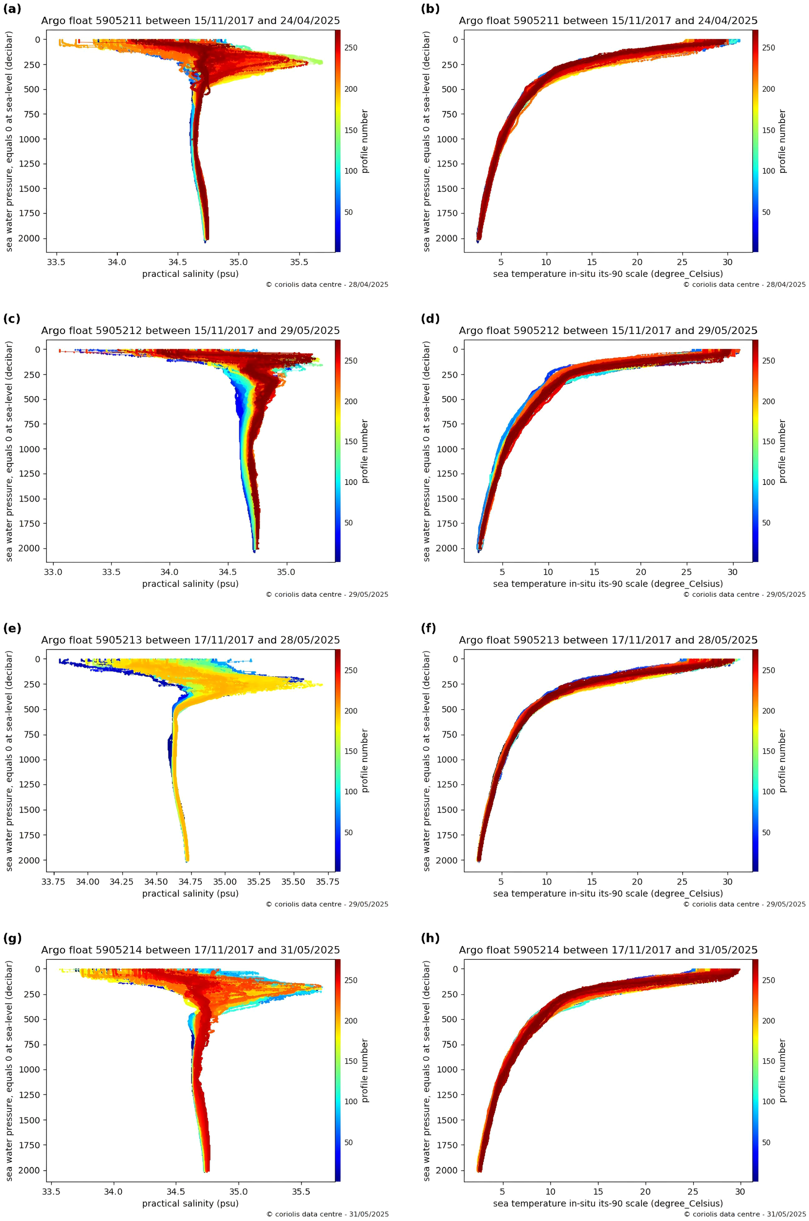
(a-h) Full-profile Argo float observations this figure presents the ocean profile observations from four Argo floats (IDs 5905211–5905214) collected between November 2017 and May 2025. It shows the variation of in situ temperature (ITS-90 scale, °C) and practical salinity (PSU) with depth (pressure, in dbar). In each subplot, color indicates the profile number, transitioning from blue (early observations) to red (later observations), thereby reflecting the temporal evolution of the dataset. Depth is plotted with 0 dbar at the surface, increasing downward. Only data from depths shallower than 130 m are used in this study. Data source: Argo float observations (IDs: 5905211–5905214), retrieved from the official Argo website [(https://argo.ucsd.edu) (https://argo.ucsd.edu)] via the Coriolis Data Center visualization tool, accessed in May 2025.© Argo Data Center. All rights reserved.
3 Methods
3.1 Basic model
Intelligent quality control of ocean buoy profile data faces two major challenges: the high cost of manual labeling and the difficulty of detecting complex anomaly patterns under dynamic ocean conditions. To address the issue of label scarcity and enhance the model’s generalization ability in handling diverse anomalies, this study adopted a semi-supervised learning (SSL) approach. SSL is a machine learning paradigm that leverages a small amount of labeled data alongside a large volume of unlabeled data, aiming to build models with strong generalization performance even in the absence of abundant annotations (Li et al., 2023). In practical applications—especially in fields such as ocean observation, remote sensing, and bioinformatics—acquiring large, high-quality labeled datasets are often expensive and labor-intensive. SSL provides a promising solution via allowing the model to learn structural patterns from labeled samples while using unlabeled data to better understand the overall data distribution, thereby improving its discriminative power and robustness in the input space.
Among SSL techniques, the Mean Teacher model is a widely recognized and effective architecture. It consists of a dual-branch neural network system: a student model and a teacher model. The teacher’s weights are continuously updated using an Exponential Moving Average (EMA) of the student’s weights, maintaining a stable learning target for the student. During training, the student model makes predictions on perturbed inputs, while the teacher model generates target outputs from the original, unperturbed inputs. The consistency between their outputs is minimized via a consistency loss, enabling the model to learn structural patterns from unlabeled data. This approach not only improves the utilization of unlabeled data but also avoids the error accumulation often observed in pseudo-labeling methods (Tarvainen and Valpola, 2017).
The core mechanism of the Mean Teacher framework lies in its use of abundant unlabeled data to drive model training, guided by a stable consistency regularization process that encourages convergence toward meaningful representations. Importantly, no explicit labels are required for the unlabeled data; instead, the model learns through “soft targets” generated by the teacher–student structure (Deng et al., 2021). As a result, the model fits well to labeled samples while also forms robust decision boundaries across the entire input distribution. This property is particularly beneficial in the presence of distributional shifts, outliers, or structurally complex data, where traditional supervised models often struggle to generalize.
In this study, we adopted the Gated Recurrent Unit (GRU) as the backbone network of the Mean Teacher framework to perform time-series modeling and feature extraction. GRU is a variant of recurrent neural networks (RNNs) designed for processing sequential data. It includes update and reset gate mechanisms that effectively capture long-term dependencies while mitigating the vanishing gradient problem (Dey and Salem, 2017).
3.2 Model design
3.2.1 Development framework and environment
The GRU–Mean Teacher model was implemented using the PyTorch deep learning framework. All model development and training procedures were conducted using Python, with the integrated development environment (IDE) set as PyCharm. The Python version used was 3.7.12. Core dependencies include pandas (version 1.3.5) and numpy (version 1.21.6), which both were managed and executed within an Anaconda virtual environment.
3.2.2 Model architecture
The model employed in this study adopted a two-layer GRU architecture (a single-layer version as illustrated in Figure 5), which was applied to both the student and teacher networks within the Mean Teacher framework. Each directional GRU contained 64 hidden units, together forming a contextual encoder capable of capturing both forward and backward information flows. This enhanced the model’s ability to perceive multi-level structural patterns across different oceanographic profile layers.
Figure 5
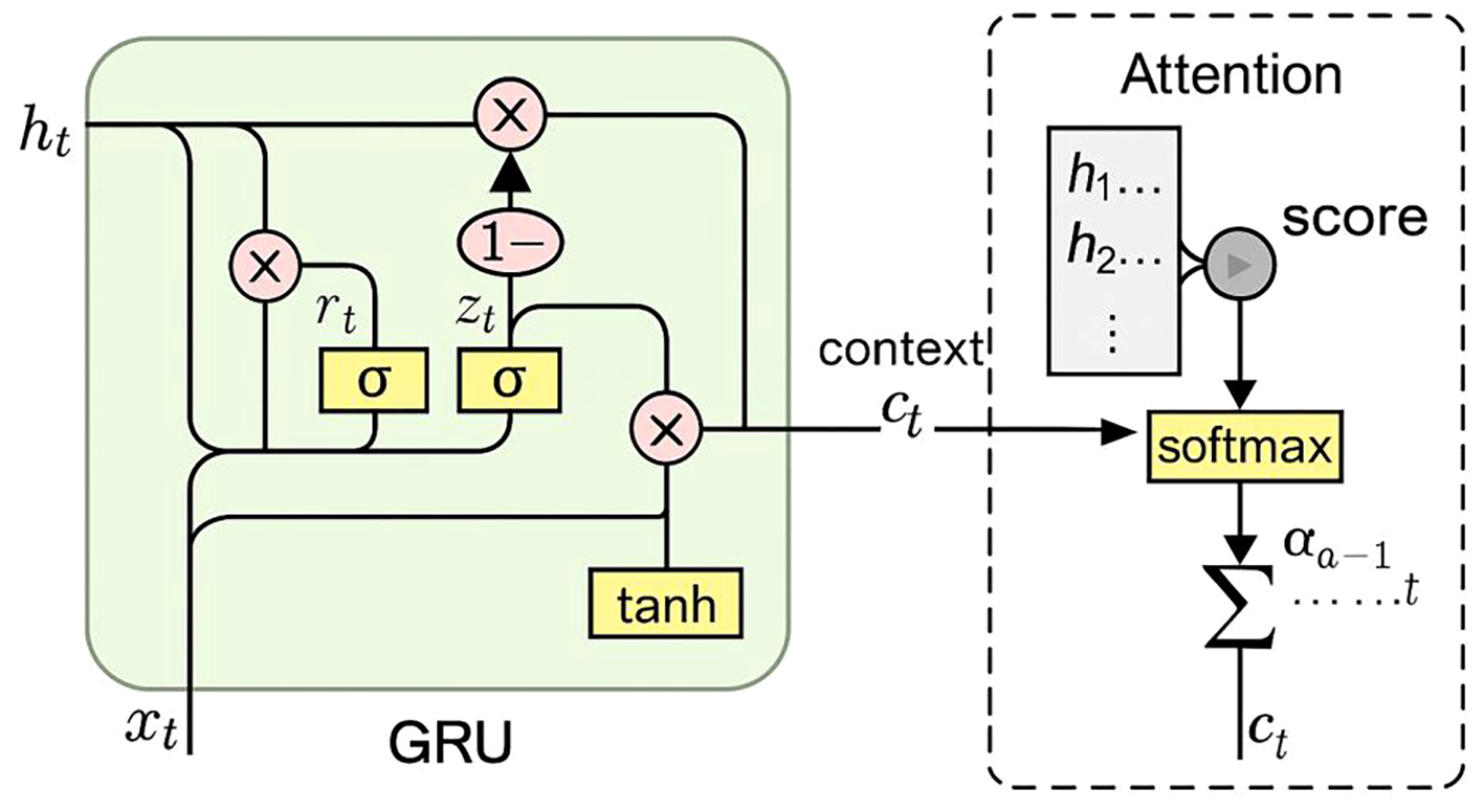
Schematic diagram of the GRU with Attention model for each layer.
On top of the GRU outputs, an attention mechanism was introduced. The primary advantage of the attention mechanism lies in its ability to simulate the way human experts examine profile plots—by focusing on layers with abrupt changes, fluctuations, or salient structural features, while down-weighting redundant or less informative regions (Zhong et al., 2018). Specifically, the model assigned a score to each GRU output using a single-layer fully connected network. These scores were normalized via the Softmax function and used as weights to compute a weighted sum of the GRU outputs. This generated a fused representation that allowed researchers to trace which layers the model “attended to” when making predictions.
After the attention mechanism, layer normalization was applied to stabilize the output. This involved computing the mean and standard deviation across the feature dimension for each sample individually, which helped mitigate numerical fluctuations arising from input variability and gradient accumulation in multi-step GRU hidden states. Such stabilization was of particular importantance when the attention-weighted context vector underwent scale shifts or becomes numerically unstable. Layer normalization thus effectively alleviated gradient oscillation issues that might occur during the joint optimization of anomaly detection (regression) and quality control classification tasks, ensuring training stability and efficient convergence.
In the Mean Teacher framework (as shown in Figure 6), GRUs were embedded in the backbone of both the student and teacher networks, and used to model and predict profile sequences (e.g., TEMP and PSAL as functions of DEPTH). During each training iteration, the student GRU processed perturbed inputs to generate predictions, while the teacher GRU produced reference outputs based on unperturbed data. These outputs were aligned via consistency loss, enhancing the model’s learning capability. Notably, the GRU served a dual role in this semi-supervised setup: it not only contributed to supervised learning objectives (e.g., predicting true labels) but also supported unsupervised consistency constraints, acting both as a feature extractor and an executor of the learning strategy.
Figure 6

Illustration of the overall architecture of the model. The blue solid lines indicate the processing flow of labeled data, while the blue dashed lines indicate that of unlabeled data.
The core idea of the Mean Teacher framework was to maintain two separate neural network models simultaneously: a student model, which underwent parameter updates and drived the main optimization process, and a teacher model, which did not participate in backpropagation. Instead, the teacher’s parameters were updated through the Exponential Moving Average (EMA) of the student’s parameters. Structurally, the student and teacher networks were identical, both comprising the aforementioned GRU + Attention architecture. The only difference lied in how their parameters were updated. Specifically, the parameters of the teacher model are updated at each training step according to Equation 1.
Here, denoted the decay factor, typically set close to 0.99, to maintain the stability of the teacher model. The essence of this strategy lied in introducing a “slow-moving” learning target for the model, allowing the teacher network’s outputs to remain smooth and robust. This facilitated the generation of high-confidence pseudo-labels, which served to guide the student model’s learning direction on unlabeled samples.
During training, the student model received a mixed input comprising both labeled and unlabeled data. For the unlabeled samples, this study implemented a “soft supervision” mechanism through two complementary strategies: on one hand, noise was added to the student model’s inputs (e.g., via Dropout or data perturbations): on the other hand, the teacher model generated stable predictions for the same inputs under noise-free conditions. The consistency loss is defined as the Mean Squared Error (MSE) between the outputs of the student and teacher models, as formalized in Equation 2.
Here, denoted the perturbed input sample, and represented the prediction function of the model. This consistency loss reflected an important cognitive assumption: if the model had a thorough understanding of the input structure, its predictions should remain consistent under input perturbations. This served not only as a form of regularization, but also as a crucial pathway for deep networks to extract underlying structures from unlabeled data.
However, in the early stages of training, the teacher model was still unstable, and the pseudo-labels it generated may lack reliability. Imposing consistency constraints too early may lead to suboptimal convergence or overly confident yet incorrect predictions. To address this issue, this study introduced the consistency ramp-up strategy (Tarvainen and Valpola, 2017), where the influence weight of the consistency loss was gradually increased during the initial training phase. This allowed the model to rely mainly on supervised signals during the first few training epochs, and to enhance the guidance from unlabeled data once the outputs of the student and teacher begin to align. Typically, followed a sigmoid or exponential growth schedule, smoothly transitioning from 0 to a predefined maximum value (e.g., 0.1) over the first 50 epochs.
3.2.3 Loss function design
To simultaneously achieve high-precision modeling of the physical structures of temperature and salinity profiles, as well as effective detection of anomalous observations, this study designed a multi-task loss function framework composed of both regression and classification objectives. This framework integrated supervised signals from labeled samples and incorporated a structured weighting mechanism together with semi-supervised consistency guidance, enabling the model to maintain strong generalization performance and stable learning even under conditions of label imbalance and observational complexity.
For the regression task, Mean Squared Error (MSE) was adopted as the optimization objective to measure the discrepancy between the model’s predicted temperature and salinity values and the original observations. Reconstruction was treated as a core task because most physical oceanographic data exhibited continuity and follow natural laws. By forcing the model to learn the patterns of “normal” profile structures, this approach essentially enhanced the model’s robustness to background noise in a self-supervised manner. In addition, to emphasize the modeling priority of salinity, the MSE loss for salinity was assigned a threefold weight. This design was motivated by observational findings indicating that salinity anomalies were generally more subtle in magnitude yet more difficult to capture with simple trend-based models, and their impacts can be significant. Therefore, reinforcing salinity reconstruction accuracy at the loss level helped the model become more sensitive to low-amplitude but high-impact anomalous behaviors.
For the classification task, a weighted Binary Cross-Entropy (BCE) loss was employed to detect anomalies in TEMP_QC and PSAL_QC labels. To address the real-world imbalance where QC = 0 (anomalous) samples were much fewer than normal ones, this study assigned a significantly higher loss weight to anomalous samples (5 for anomalies vs. 1 for normal samples). This increased the model’s “penalization capacity” for anomalies, guiding it to focus more on these rare yet critical cases during training. Furthermore, to prevent anomalous samples from dominating the gradient updates in the regression loss, their weight in the regression component was downscaled to 0.2, thereby weakening their influence on the reconstruction objective. This differentiated weighting strategy effectively established a “strategic synergy” between tasks: the regression branch focused on learning normal patterns, while the classification branch concentrated on identifying anomalous signals. Together, these components formed a complementary, rather than conflicting, multi-task framework. The total supervised loss for the labeled samples is given by Equation 3.
In the overall training objective, considering that the model needed to handle both labeled and unlabeled samples, a consistency loss was further introduced in this study, Thereby constructing the complete semi-supervised training objective function as shown in Equation 4.
Here, was a dynamic scaling factor that varied with the training progress, used to control the influence of the consistency loss at different stages of training.
In terms of the overall process, during the labeled data training phase, samples were passed through the student model and involved in both regression and classification tasks. The corresponding loss function consisted of two main components: on the one hand, the regression loss minimized the discrepancy between the model’s predicted temperature and salinity values and the true observations, thereby performing the reconstruction task; on the other hand, the classification loss used the actual TEMP_QC and PSAL_QC labels to carry out anomaly detection.
In the unlabeled data training phase, the data were likewise fed into the student model for forward propagation. However, unlike the labeled samples—which relied on supervised signals to optimize classification and regression outputs—the core of this phase lied in guiding the model to learn the underlying data structure through consistency constraints. Specifically, the student model generated predictions based on perturbed inputs, while the teacher model produced reference outputs from the same inputs without perturbation. The discrepancy between the two outputs constituted the consistency loss.
Therefore, in the training process for unlabeled data, the student model did not participate in the classification task but was still indirectly involved in the regression task through the alignment of outputs between the student and teacher models.
3.3 Train
3.3.1 Feature selection
In machine learning research, feature engineering is one of the key factors influencing algorithm performance. Appropriately selecting and designing input features is crucial for enhancing a model’s generalization ability and robustness. Specifically, in this study, based on the practical requirements of oceanographic data quality control and the characteristics of the observational data, we selected a set of representative and informative input features, as detailed below:
-
-Temperature (TEMP): Real-time temperature measurements collected by the buoy (unit: °C);
-
-Salinity (PSAL): Real-time salinity measurements collected by the buoy (unit: PSU);
-
-One-hot Encoded Season: One-hot encoded seasonal feature based on the month of observation;
-
-Temperature Gradient: The gradient of temperature with respect to depth;
-
-Salinity Gradient: The gradient of salinity with respect to depth;
-
-One-hot Encoded Depth: One-hot encoded feature indicating different depth levels.
To enhance the model’s ability to detect anomalous data, this study incorporated not only the raw physical variables directly observed by the buoy—such as temperature (TEMP) and salinity (PSAL)—but also several structured and derived features, aimed at improving the model’s perception of profile structures, seasonal variability, and contextual information. Temperature and salinity served as the fundamental variables for anomaly detection. The One-hot Encoded Season feature transformed the observation month into a one-hot vector representing the corresponding season.The temperature gradient(∂TEMP/∂DEPTH)and salinity gradient (∂PSAL/∂DEPTH) reflected the vertical continuity and rate of change within the profile data, serving as key indicators for identifying sharp transitions or abnormal jumps in the water column. Finally, since buoy data did not always provide full-depth coverage, the One-hot Encoded Depth feature transformed specific measurement depths into discrete dimensions, enabling the model to recognize the depth level of each input sample during the encoding stage (Potdar et al., 2017).
3.3.2 Data pre-processing
To ensure that the deep neural network can effectively learn both physical patterns and anomaly structures during training, this study first performed basic data cleaning and structured feature construction on the raw observational data. Specifically, filtering thresholds were set based on fundamental physical knowledge: only observations with temperature within the range of [−5, 50]°C and salinity within [1, 60] PSU were retained. This process eliminated extreme outliers and invalid placeholder values that could interfere with model gradients, improves the consistency and modelability of the overall data distribution, and prevented disruptions to the model’s convergence trajectory.
For numerical features (such as temperature, salinity, gradient terms, and interaction terms), Z-score normalization was uniformly applied to standardize the input, avoiding learning inefficiencies caused by differences in variable scales. Depth and seasonal information were processed using one-hot encoding. Each observation’s depth was discretized into five representative levels (20 m, 40 m, 60 m, 80 m, and 100 m) and encoded as a 0–1 vector. The seasonal feature was constructed based on the timestamp of each observation: by extracting the month field, each sample was assigned to one of four seasons—spring (March–May), summer (June–August), autumn (September–November), and winter (December–February). A one-hot encoding strategy was then applied to convert these discrete season categories into numerical input vectors.In practice, the procedure first extracted the month from the timestamp, then mapped each sample to its corresponding season category (indexed 0 to 3), and finally generated a binary vector of length 4 to represent seasonal information. For example, spring was encoded as [1, 0, 0, 0], summer as [0, 1, 0, 0], and so on.
To further enhance the model’s ability to capture profile structures, a sliding-window mechanism was introduced. Each observation point was combined with its preceding and succeeding neighbors to form a three-step sequence that incorporated local contextual information, resulting in a structured input tensor of size 3×12. The step size (stride) was set to 1 layer, meaning that the window shifted downward by one depth level at a time. This design ensured sufficient overlap between adjacent windows and allowed the model to capture fine-grained vertical variability. In deep learning, this approach is often referred to as local context enhancement, with the key advantage of transforming point-wise prediction into segment-based structural modeling. Consequently, the model no longer relied solely on the instantaneous state of the current point but also perceived its spatial continuity (Xu et al., 2024). Such contextual modeling is particularly critical for anomaly detection in oceanographic profiles. For example, when salinity at a given depth significantly deviates from that of adjacent layers, the model can more accurately identify this anomaly by comparing it with neighboring points within the sliding window.
3.3.3 Model training
The labeled dataset was divided into four subsets: training data (60%) is used for model parameter learning and updates; validation data (15%) is employed to optimize model hyperparameters and prevent underfitting or overfitting; testing data (10%) was used for threshold adjustment; and control data (15%) was reserved for final model performance evaluation. Unlabeled data was used during training for computing the consistency loss, guiding the student model to learn latent data structures from unlabeled samples and thereby improving generalization.
The network architecture adopted a two-layer GRU structure with 64 hidden units per layer, integrated with attention mechanisms and layer normalization to enhance feature representation and training stability. The training process was based on the Mean Teacher framework, in which the student model made predictions on perturbed inputs (e.g., with added noise), while the teacher model predicted on the same inputs without perturbations. The difference between these predictions formed the consistency loss, which encouraged the student model to align with the data distribution learned from unlabeled inputs.
In terms of the loss function, a dual-task strategy was employed, combining both regression and classification objectives. The regression loss was calculated using Mean Squared Error (MSE), with the salinity loss component weighted three times higher than that of temperature, enabling the model to be more sensitive to subtle salinity anomalies. The classification loss used weighted Binary Cross-Entropy (BCE), where significantly higher weights were assigned to anomalous samples to enhance the model’s sensitivity to rare but critical anomalies.
To avoid misleading gradients caused by the instability of the teacher model during early training, a ramp-up strategy was adopted for the consistency loss, gradually increasing its influence over time. The optimization was performed using the Adam optimizer, with an initial learning rate set to 0.001, and weight decay of 0.01 applied to control model complexity.
The model was trained for 200 epochs, with dropout applied during training to randomly deactivate a subset of neurons, thereby reducing the risk of overfitting. In the later stages of training, the Receiver Operating Characteristic (ROC) curve was used to optimize the anomaly detection threshold (Fawcett, 2006). This threshold optimization considered the class imbalance in the dataset, ensuring high efficiency and accuracy in distinguishing between normal and anomalous data. Finally, model performance was evaluated using a control dataset that was entirely excluded from training, ensuring robust assessment of the model’s generalization capability and real-world applicability.
4 Evaluation results and analysis
4.1 Performance evaluation of the model
To comprehensively evaluate the performance of the proposed semi-supervised temperature and salinity quality control model based on GRU + Attention, two classical classification evaluation metrics were introduced: the Receiver Operating Characteristic (ROC) curve and the Precision-Recall (PR) curve. These metrics respectively assessed the model’s overall discriminative capability and anomaly detection precision, providing a systematic analysis of its performance on the labeled validation dataset.
Figure 7 presented the ROC curve, where the x-axis represented the False Positive Rate (FPR) and the y-axis represented the True Positive Rate (TPR). By varying the reconstruction error threshold used by the model to determine whether a sample was anomalous or not, a series of FPR and TPR pairs were computed to form the ROC curve. The Area Under the ROC Curve (AUC) is widely used in binary classification tasks as a comprehensive performance indicator. Specifically, the closer the AUC value is to 1, the stronger the model’s discriminative ability; conversely, an AUC close to 0.5 indicates performance no better than random guessing.
Figure 7
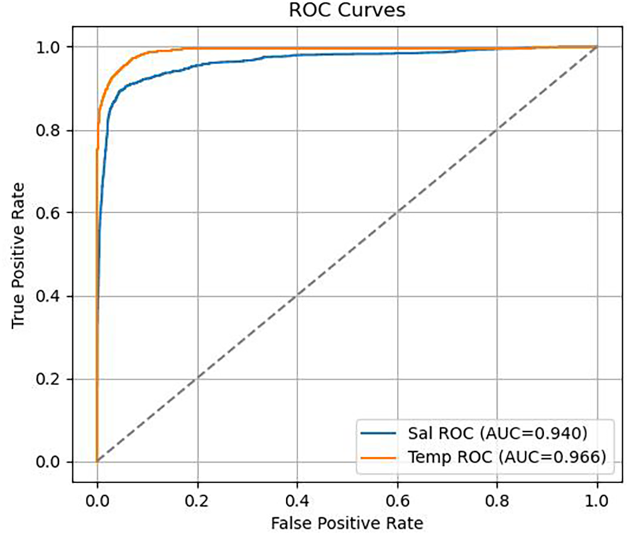
ROC curves for temperature and salinity.
In this experiment, the model achieved an ROC AUC of 0.966 for temperature data and 0.940 for salinity data, both demonstrating strong classification performance. Notably, the model showed high sensitivity and specificity in detecting salinity anomalies.
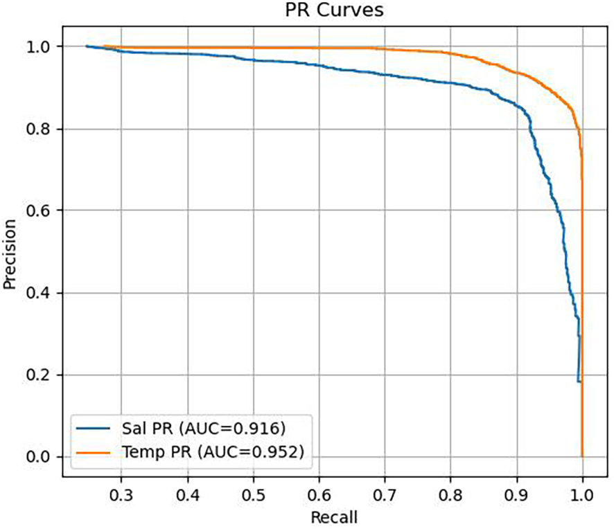
Figure 8 showed the Precision-Recall (PR) curve, where the x-axis denoted Recall and the y-axis denoted Precision. Compared to the ROC curve, the PR curve was more sensitive under conditions of extreme class imbalance (e.g., when anomalous samples were far fewer than normal ones), making it particularly valuable for anomaly detection tasks. The Area Under the PR Curve (PR AUC) reflected the model’s overall trade-off between precision and recall across all possible threshold settings.
Figure 8
PR curves for temperature and salinity.
In this study, the model achieved a PR AUC of 0.952 in the temperature anomaly detection task and 0.916 in the salinity task, both of which were considered high-performance levels. These results indicated that the model not only effectively identifies the majority of anomalous samples (high recall) but also maintained a low rate of false positives (high precision).
Specifically, a higher Recall value indicates that the model has strong sensitivity to anomalies, meaning that the majority of anomalous samples are correctly identified without being missed. Meanwhile, a higher Precision value suggests a lower false positive rate for normal samples, which is beneficial for the stable operation of downstream analysis or alert systems. Notably, in the anomaly detection task for salinity data, the PR AUC reached 0.916, further demonstrating the model’s robustness in handling salinity anomalies, which are often complex, variable, and susceptible to sensor drift. This strong performance was closely related to the training design, in which the salinity regression loss was assigned a higher weight, and the classification loss was adjusted through a weighted strategy.
Moreover, during the model evaluation phase, the input used for anomaly scoring was derived from the model’s reconstruction module, specifically the absolute error between the model’s output (predicted temperature and salinity) and the original input. Binary classification scores were then computed based on the corresponding QC labels. This evaluation method, which was based on reconstruction error rather than raw features, more accurately reflected the direct relationship between the model’s reconstruction capability and its ability to detect anomalies. It also offered a more behaviorally interpretable assessment pathway aligned with the model’s internal mechanisms.
Taken together, the analysis of both the ROC and PR curves clearly demonstrated that the proposed semi-supervised model achieved excellent performance in the task of temperature and salinity quality control. It effectively fulfilled the objective of anomaly detection and exhibited strong potential for practical applications.
4.2 Evaluation of quality control performance
To further validate the anomaly detection and classification capabilities of the proposed semi-supervised quality control model on real-world observational data, this study constructed a standard confusion matrix based on the model’s final prediction outputs and the ground-truth labels (i.e., the control dataset labels). From this matrix, four key performance metrics were derived: True Positive Rate (TPR), False Positive Rate (FPR), False Negative Rate (FNR), and True Negative Rate (TNR):
-
-TPR represented the proportion of actual normal samples that are correctly identified as normal by the model, measuring the model’s ability to recognize valid data.
-
-FPR refered to the proportion of actual anomalous samples that were incorrectly classified as normal, indicating the model’s tendency to produce false negatives for anomalies.
-
-FNR indicated the proportion of actual normal samples that were mistakenly classified as anomalous, reflecting the risk of over-flagging valid observations.
-
-TNR represented the proportion of actual anomalous samples that were correctly identified as anomalies, serving as a key indicator of the model’s anomaly detection capability.
Together, these four metrics formed the core dimensions for evaluating the classification performance of the model. By analyzing these indicators, this study provided a more granular understanding of the model’s behavior under various prediction scenarios, as well as potential risks of misclassification or missed detection.
The confusion matrix consisted of the following fundamental elements:
-
-TP (True Positive): Samples that were truly normal and correctly identified as normal;
-
-FP (False Positive): Samples that were truly anomalous but incorrectly classified as normal;
-
-FN (False Negative): Samples that were truly normal but mistakenly identified as anomalous;
-
-TN (True Negative): Samples that were truly anomalous and correctly identified as anomalous.
In the temperature quality control task, the model demonstrated excellent predictive performance (shows in Figure 9). Specifically, within the control dataset, the model correctly identified 16,750 normal samples (True Positives, TP), while 589 anomalous samples were incorrectly classified as normal (False Positives, FP). On the other hand, only 431 normal samples were mistakenly classified as anomalous (False Negatives, FN), and 2,459 anomalous samples were correctly identified (True Negatives, TN).
Figure 9

Comparison between model-predicted labels and ground-truth labels for the temperature dataset.
Based on these results, four key performance metrics were calculated (shows in Table 1):
Table 1
| TP = 16750 | FP = 589 |
| FN = 431 | TN = 2459 |
| TPR = 0.9748 | FPR = 0.1933 |
| FNR = 0.0252 | TNR = 0.8067 |
Confusion matrix results and performance metrics for temperature quality control (Temp_QC).
-
-TPR (TPR = TP/(TP + FN)) reached 97.48%, indicating that the model achieved very high coverage in detecting normal samples—most normal data were correctly recognized.
-
-FPR (FPR = FP/(FP + TN)) was 19.33%, reflecting the proportion of anomalous samples misclassified as normal, which directly related to the model’s risk of false acceptance in practical deployment.
-
-FNR (FNR = FN/(TP + FN)) was 2.52%, showing a very low probability of missing normal samples, highlighting the model’s reliability in preserving critical data.
-
-TNR (TNR = TN/(FP + TN)) reached 80.67%, demonstrating the model’s strong capability in stably identifying the majority of true anomalies.
In the salinity quality control task, the model likewise demonstrated robust performance characteristics (shows in Figure 10). It successfully identified 15,761 normal samples (TP) and 2,988 abnormal samples (TN), while 768 abnormal samples were incorrectly classified as normal (FP), and 712 normal samples were mistakenly recognized as abnormal (FN).
Figure 10
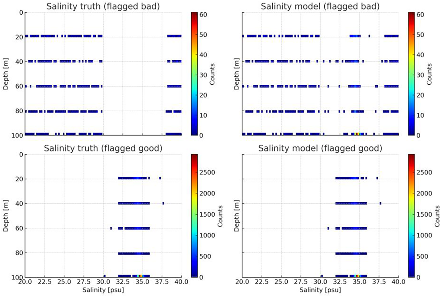
Comparison between model-predicted labels and ground-truth labels for the salinity dataset.
Further metric analysis shows that the true positive rate (TPR) reached 95.68%, indicating the model’s strong ability to correctly recognize normal data. The false positive rate (FPR) was 20.43%, slightly higher than that in the temperature detection task. This may be attributed to the salinity data exhibiting more diverse anomaly patterns and complex physical behaviors during observation, which increased the difficulty of accurate discrimination. The false negative rate (FNR) was 4.32%, meaning that the model maintained a low and acceptable level of missed detections for normal data. Meanwhile, the true negative rate (TNR) was 79.57% (shows in Table 2), suggesting that the model remained stable in identifying abnormal data—although slightly inferior to the temperature detection task, it still effectively met the fundamental requirements of anomaly detection overall.
Table 2
| TP = 15761 | FP = 768 |
| FN = 712 | TN = 2988 |
| TPR = 0.9568 | FPR = 0.2043 |
| FNR = 0.0432 | TNR = 0.7957 |
Confusion matrix results and performance metrics for salinity quality control (Sal_QC).
4.3 Manual inspection
This study also designed and implemented a systematic manual visual inspection procedure as a supplementary method for evaluating the model’s detection accuracy and generalization capability. Manual visual inspection was conducted by analysts with expertise in oceanographic observations, who professionally reviewed the quality control results of unlabeled data. During the assessment, the evaluators considered multiple factors, including historical profile trends and the current station’s environmental context, to determine whether a given data point exhibited unreasonable deviations.
Thousands of data records identified as anomalous by the model were randomly sampled and categorized by depth layers, time periods, and anomaly intensity levels. Each category was then manually verified. During this process, the observers paid special attention to the following three typical types of anomalies:
-
-Abrupt anomalies, characterized by sharp discontinuities or sudden jumps at a single depth point in the temperature or salinity profiles—often indicative of sensor failure or data writing errors.
-
-Gradual drift anomalies, where a systematic deviation appeared across the entire profile (e.g., salinity being uniformly higher by 0.3 PSU), usually associated with calibration errors.
-
-Subtle edge anomalies, which may not exhibit obvious spikes but deviate from historical trends and contradict known physical processes—these often occur near the boundary of normal conditions.
These three types of anomalies were the primary focus of manual verification and served as critical indicators for assessing the model’s comprehensive anomaly detection capability.
To quantitatively assess the consistency between model outputs and manual evaluations, this study calculated the proportion of anomalous samples identified in the unlabeled dataset. The evaluation primarily relied on monthly anomaly rate curves generated by the model on two sets of buoy profile data: the “14” dataset (from April 2014 to April 2015) and the “16” dataset (from October 2016 to January 2018), which were used to quantify the stability of anomaly detection over time.
As shown in Figure 11a, the temperature anomaly rate in Dataset14 remained consistently low throughout the observation period, indicating no abnormal fluctuations. In contrast, Figure 11c showed a slight increase in the temperature anomaly rate of Dataset16 during October 2016 and January 2018, reaching 0.068 and 0.049, respectively, which might be attributed to potential sensor disturbances during deployment and retrieval of the buoy.
Figure 11
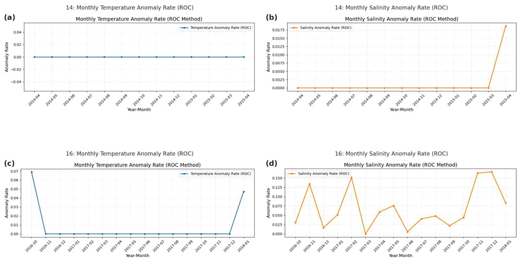
(a–d) Estimated anomaly rates for temperature and salinity in the unlabeled dataset.
In comparison, Figure 11b presented a sudden spike in the salinity anomaly rate of Dataset14 in April 2015, rising to 0.0182, which might also be related to buoy recovery activities. Meanwhile, Figure 11d showed a multi-peak pattern in the salinity anomaly rate of Dataset16, with values reaching 0.1398 in November 2016, 0.1533 in February 2017 (the highest), 0.1647 in November 2017, and 0.1662 in December 2017. Other time points, such as April 2017 (0.0621), May 2017 (0.1006), and January 2018 (0.0857), also exhibited clear upward trends.
These results indicated that the model was more sensitive to salinity anomalies, while remaining relatively conservative in detecting temperature anomalies.
From the overall feedback of the manual inspection process, the observers generally agreed that the model’s outputs were highly interpretable and reliable. After conducting manual visual inspections on the two buoy datasets in the early stages of the study, it was found that when the buoy was stably deployed and in good operational condition, the likelihood of abnormal values appearing in the sensor-recorded profiles was relatively low. In other words, the presence of genuine anomalies in the data itself was sparse and limited.
Therefore, the near-zero monthly anomaly rates observed in the temperature detection results (as shown in Figures 11A, C) serve as a clear indication of the model’s effective ability to distinguish true anomalies. Regarding salinity, the fluctuating anomaly rates in the Dataset16 (Figures 11B, D) were partially confirmed through manual inspection: some anomalies were indeed false positives, caused by the model misclassifying boundary samples. This was likely due to the semi-supervised model’s heightened sensitivity to subtle deviations in the absence of labels, especially for salinity, where tolerance for minor shifts was lower.
However, another important factor was the aftermath of the strong El Niño event in 2015, which led to a prolonged period of low-salinity conditions during recovery. In such cases, the identified salinity anomalies reflected genuine physical changes in ocean structure, rather than conventional data quality issues. Despite this, the researchers still recommended using the model’s outputs as the primary basis for manual review, with flagged anomalies being prioritized for further expert verification.
As described above, during the in-depth analysis of the model’s anomaly detection results, it was observed that some data samples consistently identified as anomalous over extended periods were, upon manual verification, not caused by data errors or sensor malfunctions, but rather by actual physical processes associated with intrusions of anomalous water masses. The hydrographic characteristics of such water masses often exhibited significant numerical deviations from the typical background fields—for example, low temperature with high salinity, high temperature with low salinity, or normal temperature with low salinity. As a result, the model automatically classified them as anomalies based on reconstruction error and probabilistic judgment mechanisms.
However, from the perspective of ocean dynamical processes, such water masses represent genuine physical phenomena and should be considered “atypical but physically plausible” observations. These cases should not be simply categorized as invalid data or erroneous measurements, but rather interpreted in the broader context of environmental variability and oceanographic events.
Taking the 100-meter depth observational data from 2016 as an example, the model consistently labeled this depth layer as anomalous over several consecutive periods.
However, manual verification through profile visualization and comparison with historical data from the same period revealed that these “anomalieswere” actually caused by a significant low-salinity water mass intrusion event. This water mass induced a marked decrease in salinity in the vertical profile, which deviated substantially from the deep-water distribution patterns learned by the model. Although these data points were statistically classified as outliers, from an oceanographic perspective, they represent important variations in the observed environment.
This phenomenon not only suggested the need to incorporate stronger physical priors during model training to avoid misclassifying real oceanic processes, but also highlighted the potential value of semi-supervised learning models in oceanographic research. Such models can be used not only for anomaly elimination and quality control but also as auxiliary tools for exploring atypical oceanographic events.
By reviewing model-identified anomalies and verifying them manually, researchers can extract samples that may correspond to unusual water masses, internal waves, oceanic fronts, or sudden hydrographic structure changes. These insights serve as important clues for subsequent physical process modeling and mechanism analysis. In fact, such “informative misclassifications” may carry greater scientific significance than accurate labels themselves, demonstrating the unique potential of semi-supervised quality control models in supporting exploratory ocean analysis and anomaly detection.
5 Comparative analysis of models
Although deep learning has demonstrated strong data modeling capabilities across various fields in recent years, its applications in ocean data quality control (QC) remain relatively limited. Existing deep learning models that are directly applicable to QC tasks are few in number, differ significantly in architecture and training strategies, and lack systematic comparison and evaluation. To thoroughly investigate the adaptability and performance differences of various deep learning paradigms in buoy-based QC tasks, this study proposes a deep neural network QC model that integrates GRU for sequential modeling with the semi-supervised Mean Teacher framework, balancing temporal dynamics with adaptability to label scarcity. This model is systematically compared with the currently representative fully supervised model—SalaciaML, which is based on a multilayer perceptron (MLP) architecture. The SalaciaML model uses a two-layer fully connected MLP structure, taking static input features such as temperature, depth, and gradient. It relies on large-scale, high-quality manually labeled datasets and is trained in a fully supervised manner. Primarily applied in well-observed regions like the Mediterranean Sea, where annotated data are abundant, this model achieves high classification accuracy. In previous evaluations, it achieved a ROC-AUC of 0.952 for temperature anomaly detection, with TPR (true positive rate) of 89% and TNR (true negative rate) of 86%, performing well in binary classification tasks for good/bad samples. However, SalaciaML has several limitations in terms of model design and scalability. First, it entirely depends on labeled data and cannot learn effectively from unlabeled samples, significantly limiting its application in data-sparse regions. Second, it supports QC only for the temperature variable and lacks generalizability to other key parameters such as salinity and density. Third, due to its use of static features as input, it fails to capture profile structure and temporal dynamics, making it less effective in identifying weak anomalies or nonlinear profile transitions.
To address these issues, the GRU + Mean Teacher model proposed in this study introduces a semi-supervised learning mechanism that overcomes dependence on large volumes of labeled data. The key advantage of this model lies in its ability to jointly train with a small number of labeled samples and a large number of unlabeled observations. It uses a teacher network to generate high-confidence pseudo-labels for unlabeled samples and leverages consistency regularization to guide the student model in gradually approximating a reliable anomaly classification boundary. Structurally, the model adopts a two-layer GRU architecture to process vertical profile sequences (e.g., temperature and salinity as functions of depth), and integrates an attention mechanism at the output to enhance sensitivity to local anomalies. Moreover, a sliding window mechanism is used to construct contextual feature sequences, allowing the model to capture vertical trends between adjacent layers, thereby improving its ability to detect structural anomalies such as thermocline displacement, edge drift, or subtle outliers.
In performance evaluations, the semi-supervised model achieved an average ROC-AUC of 0.953 on the validation set, with a TPR of 96.58% and a TNR of 80.12%, demonstrating stable and reliable performance in both temperature and salinity anomaly detection. Furthermore, even when applied to a large volume of unlabeled data using pseudo-labels for auxiliary evaluation, the model maintained approximately 90% accuracy, reflecting strong label efficiency and generalization capability (shows in Table 3). In contrast, although SalaciaML achieved comparable results in some metrics, its applicability is limited to the temperature variable and is not effective on unlabeled data.
Table 3
| Comparison dimension | SalaciaML model | Proposed model (this study) |
|---|---|---|
| Type of Data Used | Only Labeled Data (Fully Supervised) | Labeled+ Unlabeled Data (Semi-supervised, 1:5 ratio) |
| QC Parameters | Temperature | Temperature, Salinity |
| ROC-AUC | 0.952 | 0.953 (Average) |
| True Positive Rate (TPR) | 89% | 96.58% |
| True Negative Rate (TNR) | 86% | 80.12% |
Model comparison.
It is worth noting that despite the proposed model achieving excellent performance in TPR, the relatively lower TNR indicates some limitations in comprehensive anomaly detection. Several factors contribute to this lower TNR: First, from the instrumentation perspective, the moored buoys used in this study are equipped with high-performance CTD sensors from Sea-Bird (USA), which offer excellent accuracy, stability, and resistance to interference. These sensors rarely produce systematic errors or observation faults under normal operating conditions, resulting in a very low proportion of true anomalies in the raw data. This leads to pronounced class imbalance in the training set. Although sample weighting was employed to enhance the model’s focus on anomaly classes, the model still tends to adopt conservative predictions near the decision boundary, leading to missed weak anomalies. Second, some anomalies exhibit subtle variations or indistinct boundaries in the profile, making them prone to misclassification as normal fluctuations—this is particularly common in depth ranges with highly continuous profiles. Additionally, the consistency regularization in the Mean Teacher architecture enforces prediction invariance under perturbations. To avoid systematic bias due to false positives, the model adopts a more conservative strategy when dealing with borderline cases. While this “conservative recognition” enhances overall prediction stability, it can limit the model’s ability to detect weak or concealed anomalies.
More importantly, the flexibility of the GRU + Mean Teacher model in training strategy and data adaptability significantly enhances its scalability for real-world ocean observation tasks. When facing platforms deployed in different regions or under varying observation conditions, the model can rapidly adapt and optimize using only a small number of manually QC’ed samples, making it especially suitable for remote marine areas with scarce annotations but high monitoring demands.
It should be noted that the performance metrics of SalaciaML are directly quoted from its original publication, where the model was trained on a large Mediterranean dataset. Therefore, these results are not strictly comparable with our re-trained models on Argo and Bailong buoy data, and they are provided only as a qualitative reference to highlight methodological differences.
6 Conclusion
This study addresses the challenge of quality control for buoy-based ocean profile data by proposing a deep learning QC approach that combines the sequential modeling capabilities of GRU with the semi-supervised Mean Teacher framework. The method is designed to overcome the limitations of both traditional QC techniques and existing deep learning models, particularly their weak ability to detect complex anomaly patterns and their strong reliance on manually labeled data. The study utilized data from moored buoys and Argo profiling floats, constructing high-dimensional structured input features, including temperature, salinity, pressure, depth, gradients, interaction terms, seasonal encodings, and depth one-hot vectors. A sliding window mechanism was incorporated to enhance contextual modeling capability.
In terms of model architecture, GRUs were employed to extract sequential features from vertical profiles, combined with an attention mechanism to highlight key layers, and layer normalization was applied to stabilize the multi-task learning process. During training, the model adopted the Mean Teacher framework, using consistency regularization to guide learning from unlabeled data when only partial QC labels were available, thereby improving the model’s generalization performance. The loss function was designed with a joint optimization strategy combining regression errors for temperature and salinity and classification loss, with higher weights assigned to salinity and anomalous samples in the classification task, thus reinforcing the learning focus on critical anomalies.
Experimental results showed that the model achieved excellent performance on ROC and PR curve evaluations, with both temperature and salinity AUC values exceeding 0.94 and strong PR-AUC scores. In the confusion matrix, TPR exceeded 90%, and the model reached approximately 90.0% consistency with human visual assessments. More importantly, the model demonstrated high sensitivity to weak anomalies, structural shifts, and water mass intrusions, suggesting its potential for exploring underlying physical processes.
However, several aspects remain to be further investigated and optimized for practical deployment and cross-regional application. Firstly, the current model still primarily relied on statistical deviations when identifying anomalies, which may lead to misclassification of physically valid but statistically abnormal events (e.g., water mass intrusions or frontal thermoclines). Future improvements may include incorporating more physical constraints, such as vertical stability criteria (N²), mixed layer depth, and other ocean dynamical parameters, to guide the neural network with physical priors. Secondly, although the model performed well on the control dataset, it still faces challenges of data sparsity and feature shift in ultra-deep or low-frequency regions. Future work should explore adaptive layer normalization, meta-learning, or domain adaptation techniques to enhance cross-platform generalization. Third, the current model treated temperature and salinity anomalies within a unified architecture, while their underlying physical mechanisms and anomaly behaviors differ significantly. In future designs, multi-branch networks or task-decoupling mechanisms may be introduced for more targeted modeling strategies. Furthermore, to improve model interpretability, attention-based or SHAP-based explainable learning frameworks can be incorporated to assist expert decision-making and model refinement. On the deployment side, the model could be integrated with ocean observation systems through embedded QC modules or edge-computing units, enabling near real-time quality control and feedback at the buoy level, and facilitating a closed-loop system of observation–evaluation–feedback–optimization. Finally, in response to the increasing heterogeneity of global multi-source oceanographic data, future efforts should move toward multi-modal collaborative learning, integrating satellite, meteorological, and auxiliary datasets to improve the model’s spatial adaptability and intelligence level.
Statements
Data availability statement
The original contributions presented in the study are included in the article/Supplementary Material. Further inquiries can be directed to the corresponding author.
Author contributions
WS: Methodology, Software, Data curation, Investigation, Writing – original draft, Visualization, Conceptualization, Validation. CN: Funding acquisition, Writing – review & editing, Writing – original draft, Supervision, Formal analysis, Project administration, Data curation, Conceptualization, Resources, Methodology. BM: Writing – review & editing, Methodology. CL: Writing – review & editing, Writing – original draft, Data curation. HL: Data curation, Writing – review & editing. ZY: Writing – review & editing, Supervision. LZ: Writing – review & editing, Investigation.
Funding
The author(s) declare financial support was received for the research and/or publication of this article. This work was supported by the National Key Research and Development Program of China (Grant number 2022YFC3104301); Deployment of a Deep-Sea Moored Buoy (Grant number B23202318101).
Conflict of interest
The authors declare that the research was conducted in the absence of any commercial or financial relationships that could be construed as a potential conflict of interest.
Generative AI statement
The author(s) declare that no Generative AI was used in the creation of this manuscript.
Any alternative text (alt text) provided alongside figures in this article has been generated by Frontiers with the support of artificial intelligence and reasonable efforts have been made to ensure accuracy, including review by the authors wherever possible. If you identify any issues, please contact us.
Publisher’s note
All claims expressed in this article are solely those of the authors and do not necessarily represent those of their affiliated organizations, or those of the publisher, the editors and the reviewers. Any product that may be evaluated in this article, or claim that may be made by its manufacturer, is not guaranteed or endorsed by the publisher.
Supplementary material
The Supplementary Material for this article can be found online at: https://www.frontiersin.org/articles/10.3389/fmars.2025.1661373/full#supplementary-material
References
1
Core Argo Data Management Team (2021). Delayed-mode quality control manual (Version 3.1) (France: Argo Data Management).
2
Deng J. Li W. Chen Y. Duan L. (2021). “ Unbiased mean teacher for cross-domain object detection,” in 2021 IEEE/CVF Conference on Computer Vision and Pattern Recognition (CVPR), Nashville, TN, USA. Piscataway, NJ: IEEE4089–4099. doi: 10.1109/CVPR46437.2021.00408
3
Dey R. Salem F. M. (2017). “ Gate-variants of Gated Recurrent Unit (GRU) neural networks,” in 2017 IEEE 60th International Midwest Symposium on Circuits and Systems (MWSCAS), Boston, MA, USA. Piscataway, NJ: IEEE1597–1600. doi: 10.1109/MWSCAS.2017.8053243
4
Fawcett T. (2006). An introduction to ROC analysis. Pattern Recognition Lett.27, 861–874. doi: 10.1016/j.patrec.2005.10.010
5
Hill K. Moltmann T. Meyers G. Proctor R. (2015). The Australian integrated marine observing system (IMOS). Marine Technology Society Journal, 44(6), 65–72. doi: 10.4031/MTSJ.44.6.13
6
Huang W.-J. Yang B.-F. Lu H.-G. Wei C.-M. (2023). Research on meteorological data quality control methods based on BP neural network. J. Chengdu Univ. Inf. Technol.38, 392–397. doi: 10.16836/j.cnki.jcuit.2023.04.003
7
Kent E. C. Rayner N. A. Berry D. I. Eastman R. Grigorieva V. G. Huang B. et al . (2019). Observing requirements for long-term climate records at the ocean surface. Front. Mar. Sci.6. doi: 10.3389/fmars.2019.00441
8
Kolukula S. S. Murty P. L. N. (2025). Enhancing observations data: A machine−learning approach to fill gaps in the moored buoy data. Results Eng.26, 104708. doi: 10.1016/j.rineng.2025.104708
9
Leahy T. P. Llopis F. P. Palmer M. D. Robinson N. H. (2018). Using neural networks to correct historical climate observations. J. Atmospheric Oceanic Technol.35, 2053–2059. doi: 10.1175/JTECH-D-18-0012.1
10
Lei F. Wan Y. Shang S. (2022). Study on quality control process and method of surface environmental elements of marine buoys. J. Ocean Technol. (China)41, 10–25. doi: CNKI:SUN:HYJS.0.2022-04-002
11
Li Y. Xu C. Tang X. Li X . (2023). Semi-supervised learning theory and applications. Acta Automatica Sin.49, 899–911. doi: 10.16507/j.issn.1006-6055.2022.07.001
12
Li T. Zhang C. Zhang S. Lu Z. (2018). An association rule–based marine meteorological data quality control algorithm using interestingness measures. Modern Electronic Technol.41, 138–142. doi: 10.16652/j.issn.1004-373x.2018.22.034
13
Li X. Zou D. Feng W. Xie W. Shi L. (2019). Study of quality control methods for moored buoys observation data,” 2019 international conference on meteorology observations (ICMO). Chengdu China2019, 1–4. doi: 10.1109/ICMO49322.2019.9026114
14
Liu S. H. Chen M. C. Dong M. M. Gao Z. G. Zhang J. L. Wu S. Q. et al . (2016). A practical quality-control method for outliers in marine buoy data. Mar. Sci. Bull.35, 264–270. doi: CNKI:SUN:HUTB.0.2016-03-005
15
Liu Y.-L. Wang G.-S. Hou M. Xu S.-S. Miao Q.-S. (2021). Application of deep learning in quality control of sea temperature observation data. Mar. Sci. Bull.40, 283–291. doi: CNKI:SUN:HUTB.0.2021-03-005
16
Mieruch S. Demirel S. Simoncelli S. Schlitzer R. Seitz S. (2021). SalaciaML: A deep learning approach for supporting ocean data quality control. Front. Mar. Sci.8. doi: 10.3389/fmars.2021.61174
17
Ning C.-L. Xue L. Jiang L. Li C. Gao F. Yu W.-D. (2022). A solution for global communication system sharing of Bailong buoy data. J. Hohai Univ. (Natural Sci. Edition)50, 91–95. doi: CNKI:SUN:HHDX.0.2022-03-012
18
Potdar K. Pardawala T. Pai C. (2017). A comparative study of categorical variable encoding techniques for neural network classifiers. Int. J. Comput. Applications.175, 7–9. doi: 10.5120/ijca2017915495
19
Sprintall J. Wijffels S. E. Molcard R. Jaya I. (2009). Direct estimates of the Indonesian Throughflow entering the Indian Ocean: 2004–2006. J. Geophys. Res.114, C07001. doi: 10.1029/2008JC005257
20
Sugiura N. Hosoda S. (2020). Machine learning technique using the signature method for automated quality control of Argo profiles. Earth Space Sci.7, e2019EA001019. doi: 10.1029/2019EA001019
21
Tarvainen A. Valpola H. (2017). “ Mean teachers are better role models: Weight-averaged consistency targets improve semi-supervised deep learning results,” in Proceedings of the 31st International Conference on Neural Information Processing Systems (NIPS’17) ( Curran Associates Inc., Red Hook, NY, USA), 1195–1204.
22
Wang Y.-Z. Tao W. Lu S.-Y. (2024). Preliminary study of a neural network–based quality control method for meteorological observation data during the “return of the south” phenomenon. Meteorological Res. Appl.45, 37–44. doi: 10.19849/j.cnki.CN45-1356/P.2024.2.06
23
Wang H.-Z. Zhang R. Wang G.-H. An Y.-Z. Jin B.-G. (2012). Quality control techniques for Argo buoy temperature and salinity profile observation data. Chin. J. Geophysics55, 577–588. doi: CNKI:SUN:DQWX.0.2012-02-019
24
Wen Y. (2014). Study on the quality control of marine environment observation data. Agric. Network Inf.2), 35–38. doi: CNKI:SUN:JSJN.0.2014-02-011
25
Wimart-Rousseau C. Steinhoff T. Klein B. Bittig H. Körtzinger A. (2024). Technical note: assessment of float pH data quality control methods – a case study in the subpolar Northwest Atlantic Ocean. Biogeosciences21, 1191–1211. doi: 10.5194/bg-21-1191-2024
26
Wong A. P. S. Wijffels S. E. Riser S. C. Pouliquen S. Hosoda S. Roemmich D. et al . (2020). Argo data 1999–2019: two million temperature-salinity profiles and subsurface velocity observations from a global array of profiling floats. Front. Mar. Sci.7. doi: 10.3389/fmars.2020.00700
27
Xu S. Chen S. Xu R. Wang C. Lu P. Guo L. (2024). Local feature matching using deep learning: A survey. Inf. Fusion.107, 102344. doi: 10.1016/j.inffus.2024.102344
28
Xu M. Nian F. Chen K. Gou Z. Huang C. Li Z. (2021). Application of artificial intelligence techniques in the quality control of meteorological observation data. Available online at: https://kns.cnki.net/kcms2/article/abstract?v=GkDm8A2i92VHicy7BIo1TP8BenkyoSJn_6jOElPsx8XWk4ulFNNuVnUAka5B20rwhltWOpk6Xa1rtTONz1B5X5nWZ747CiRxEDUSCZog7OzVLjLM8LKA4da_9pWDtunEusoexttj3AxRBplhxHK3mTSEN8HBAWgYEHCPAuM5Tv4QjHjMuRBYTltiD-ed7dG9&uniplatform=NZKPT&language=CHS (Accessed June 22, 2025).
29
Zhang B. Cheng L. Tan Z. Gouretski V. Li F. Pan Y. et al . (2024). CODC-v1: A quality-controlled and bias-corrected ocean temperature profile database from 1940–2023. Sci. Data11, 666. doi: 10.1038/s41597-024-03494-8
30
Zhong G. Yue G. Ling X. (2018). Recurrent attention unit. arXiv preprint arXiv:1810.12754. arXiv:1810.12754.
31
Zhu X. Yoo W. S. (2016). Dynamic analysis of a floating spherical buoy fastened by mooring cables. Ocean. Eng.121, 462–471. doi: 10.1016/j.oceaneng.2016.06.009
Summary
Keywords
data quality control, GRU, mean teacher, buoy profile data, ocean observations
Citation
Shao W, Ning C, Ma B, Li C, Li H, Yao Z and Zeng L (2025) Intelligent quality control of ocean buoy profile data using a GRU-mean teacher framework. Front. Mar. Sci. 12:1661373. doi: 10.3389/fmars.2025.1661373
Received
08 July 2025
Accepted
13 October 2025
Published
06 November 2025
Volume
12 - 2025
Edited by
Yang Ding, Ocean University of China, China
Reviewed by
Xuefeng Zhang, Tianjin University, China
Wen Zhang, National University of Defense Technology, China
Updates
Copyright
© 2025 Shao, Ning, Ma, Li, Li, Yao and Zeng.
This is an open-access article distributed under the terms of the Creative Commons Attribution License (CC BY). The use, distribution or reproduction in other forums is permitted, provided the original author(s) and the copyright owner(s) are credited and that the original publication in this journal is cited, in accordance with accepted academic practice. No use, distribution or reproduction is permitted which does not comply with these terms.
*Correspondence: Chunlin Ning, clning@fio.org.cn
Disclaimer
All claims expressed in this article are solely those of the authors and do not necessarily represent those of their affiliated organizations, or those of the publisher, the editors and the reviewers. Any product that may be evaluated in this article or claim that may be made by its manufacturer is not guaranteed or endorsed by the publisher.