Abstract
In the North Pacific Ocean off the Kamchatka Peninsula, nonlinear internal waves (NLIWs) are still studied insufficiently. The purpose of the study was to establish patterns in the distribution of NLIW characteristics and the reasons for their significant variability. The study used Sentinel-1 radar images from 2015 to 2024, along with data from the FESOM-C tidal model, Landsat 8, Sentinel-2, and estimates of Kamchatka walleye pollock population. In total, 3,895 NLIW events were identified, revealing “hot spots” with high wave activity, mainly east of the Fourth Kuril Strait, on Kamchatka’s shelf, and around the Shipunsky Peninsula. NLIW characteristics obtained from satellite observations were supplemented by in-situ measurement near the Shipunsky Peninsula. NLIWs peaked in summer and were least active in winter. The maximum occurrence within а year was linked to the strong subsurface pycnocline, intensified tidal currents, and weak winds. “Hot spots” coincided with areas of strong diurnal tidal currents, suggesting that topographically trapped diurnal internal tide generates many NLIWs. Results also demonstrate NLIW influence on chlorophyll-a distribution and their potential role in supporting feeding base of juvenile walleye pollock, indicating the importance of internal waves in shaping the local ecosystem.
1 Introduction
Nonlinear internal waves (NLIWs) are commonly observed in coastal regions throughout the World Ocean and play a significant role in horizontal and vertical exchange processes in the upper ocean layer (Helfrich and Melville, 2006; Jones et al., 2020; Lucas and Pinkel, 2020). The shelf and steep continental slope adjacent to the Kamchatka Peninsula and the northern Kuril Islands on the Pacific Ocean are no exception. NLIWs in this area have been identified through both satellite observations (Etkin and Srnirnov, 1992; Lavrova et al., 1999; Serebryany, 2000; Jackson, 2004) and in situ measurements (Pao and He, 2002; Pao and Serebryany, 2005; Sabinin and Serebryany, 2007; Svergun and Zimin, 2020; Svergun et al., 2023). Previous studies have shown that in this region NLIWs may form as a result of the disintegration of internal diurnal tides (Svergun et al., 2023). Simulations using a nonlinear two-dimensional (in vertical section) model of inviscid, incompressible stratified flow with climatological data from World Ocean Atlas 2018 (WOA18) and smoothed analytical bathymetry for the Avacha Bay (Shcherbakova et al., 2024) demonstrate that NLIWs can be generated by the disintegration of internal tidal waves over steep topography, irrespective of the tidal forcing period. However, in the study region NLIW generation can be also influenced by other mesoscale factors. These include the formation of nonstationary internal lee waves arising when critical (in terms of the Froude number) tidal flows interact with bottom inhomogeneities (Itoh et al., 2014), the interaction of internal wave energy beams with the surface pycnocline (Sabinin and Serebryany, 2007) and instabilities of large-scale meanders of the Kuril-Kamchatka Current (Lavrova et al., 1999; Svergun and Zimin, 2020).
The Kuril-Kamchatka Current are the cold current on shelf and continental slope along of east coast of the Kamchatka Peninsula and the North Kuril Islands and, together with the Oyashio Current and the Alaska Stream, is part of the Western Pacific Subarctic Gyre. Complex bathymetry and variable wind regime are the reason that meanders and eddies consistent features of the Kuril-Kamchatka Current which have a significant impact on the hydrological structure of the region’s waters (Andreev and Pipko, 2022; Zimin et al., 2024). With the exception of shallow waters, the vertical stratification of waters belongs to the Pacific type of subarctic structure. This structure consists of three layers: seasonal surface layer, cold subsurface layer and warm intermediate layer. In summer, the temperature reaches 10–12°C with a salinity of about 33 psu in the heated surface layer of 10–30 m thick. Under it to a depth of 200–300 m there is a cold subsurface layer with a core of minimum temperature of 0–2°C and a smooth change in salinity to 33.5 psu. Below, the temperature and salinity increase rapidly reaching stable values of about 4 °C and 34.5 psu at depths of 400–500 m throughout the year. During the cold season, the surface layer disappears due to cooling, especially in the shelf zone where already in December the water temperature becomes homogeneous from the surface to the bottom. In winter, a uniform cold layer is formed, the temperature of which can reach negative values. The stability of the water column in the upper layers is ensured mainly by salinity. In shallow areas of the shelf and in the Kuril Straits, intense tidal currents can form vertically mixed stationary zones during all seasons (Shevchenko et al., 2025; Konik et al., 2024).
An analysis of satellite remote sensing data for the year 2019 by Svergun and Zimin (2020) showed that signatures of NLIWs were most frequently observed across all seasons in the following areas: east of the Fourth Kuril Strait, near Cape Lopatka, over the southeastern shelf of the Kamchatka Peninsula, around the Shipunsky Peninsula, and in the southern part of the Kronotsky Bay (Figure 1). According to the terminology used by Sabinin and Serebryany (2007), these regions can be classified as “hot spots” in the internal wave field. However, the total number of detected NLIWs in the study area varied significantly throughout 2019 with the lowest number of surface manifestations recorded between January and March and the highest between July and September. A subsequent study of Sentinel-1 radar imagery for August during the period 2017-2021revealed substantial interannual variability in the number of observed NLIW manifestations in the region (Svergun et al., 2023). This raises questions about the reliability of earlier assessments regarding the stationarity of internal wave “hot spots” and the robustness of NLIW characteristics inferred from single-year datasets. The availability of multi-year Sentinel-1 SAR images archives now provides an opportunity to derive more robust estimates of the spatial and temporal occurrence of NLIWs and their properties, as well as to investigate the underlying causes of their variability.
Figure 1
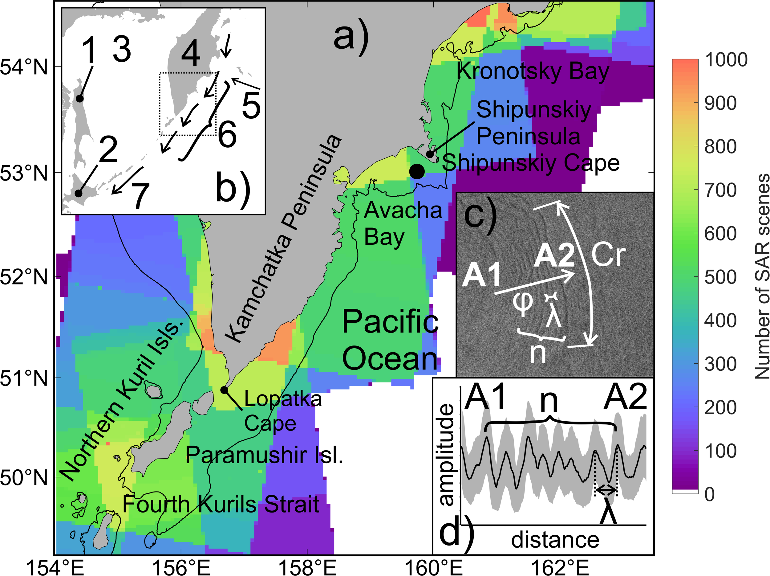
Study region. (a) Coverage of SAR images for all years from 2015 to 2024; the black dot marks the location of the in situ measurement site. The black contour indicates the 200 m isobath. (b) Schematic of the general circulation in the studied region. The dashed rectangle indicates the area shown in panel (a). 1 – Sakhalin Island, 2 – Hokkaido Island, 3 – Sea of Okhotsk, 4 – Kamchatka Peninsula, 5 – Alaska Stream, 6 – Kuril-Kamchatka Current, 7 – Oyashio Current. (c) Surface manifestation of NLIWs on SAR image and wave parameters; Cr – length of the leading crest, λ – wavelength, φ – propagation direction, n – number of waves in the packet, A1-A2 – cross-section. (d) Schematic illustration of сross-section of radar signal intensity across the NLIWs manifestation shown in panel (c). The thick black line represents the averaged signal intensity, while the gray area indicates the variability range along the entire extent of the NLIWs.
The study by Svergun et al. (2023) notes that areas of frequent NLIW occurrence (“hot spots”) on the eastern Kamchatka shelf and in the Kronotsky Bay coincide with the spawning grounds and early development areas of the eastern Kamchatka population of walleye pollock (Gadus chalcogrammus, Pallas, 1814), as reported by Buslov (2008). In a synthesis of recent data on key spawning regions and the state of the spawning stock of Eastern Kamchatka pollock based on long-term observations, the study by Varkentin and Saushkina (2022) highlights that the depth of peak spawning activity in submarine canyons varies. Furthermore, results from a targeted field experiment conducted in the canyons of the Avacha Bay (Konik et al., 2024) demonstrated a consistent relationship between changes in the vertical distribution of pollock eggs and diurnal and semidiurnal thermocline oscillations. These findings support the hypothesis that variability in hydrological conditions associated with internal wave activity may influence pollock egg distribution in this region.
Previous studies have reported that internal waves can redistribute concentrations of biogenic material and plankton (Vázquez et al., 2009; Shroyer et al., 2010; Navrotsky et al., 2012; Muacho et al., 2013; Nishino et al., 2015; Villamaña et al., 2017; Reid et al., 2019; Garwood et al., 2020; Ma et al., 2023; Guan et al., 2023), ultimately affecting the distribution and survival of commercially important marine organisms (Ezer et al., 2010; Embling et al., 2013; Greer et al., 2014; Bondur et al., 2020; McBride et al., 2024). This suggests that information on the interannual variability of NLIW may be of considerable relevance for fisheries management in this region. To date, no studies have investigated the interannual variability of NLIW across different seasons with a focus on their biological impacts in the study area.
The objective of this study is to obtain statistically robust estimates of intra-annual and seasonal variability in nonlinear internal waves characteristics in the Pacific waters adjacent to the Kuril-Kamchatka region and to identify the underlying drivers of this variability. The analysis will be based on the processing of available radar imagery from 2015 to 2024, supported by outputs from a regional tidal model and in situ data. The discussion section of the paper will explore the relationship between NLIW manifestations, chlorophyll-a concentration, and the recruitment of the eastern Kamchatka walleye pollock (Gadus chalcogrammus) population.
2 Methods
2.1 Satellite observations
NLIWs signatures were identified in synthetic aperture radar images (SAR images) acquired by the Sentinel-1A and Sentinel-1B satellites, operating in the C-band, using Interferometric Wide swath mode with spatial resolution of 20 m and swath width of 250 km. The satellite images were downloaded from the Alaska Satellite Facility. A total of 3491 SAR images were available for the period from January 2015 to December 2024. The spatial distribution of SAR image coverage across the study area is shown in Figure 1.
As shown in Figure 1a, the highest satellite data availability (over 700 SAR images over 10 years) is observed in the area of the Fourth Kuril Strait, the southeastern shelf of the Kamchatka Peninsula, and the northern part of the Kronotsky Bay. The continental shelf and upper continental slope are covered by 300 to 400 SAR scenes in ten years, while the open-ocean region beyond the shelf is covered by fewer than 200 scenes in ten years.
The SAR images were processed using the Sentinel Application Platform (SNAP) software developed by the European Space Agency, which is freely distributed under the GNU General Public License v3 (https://step.esa.int/main/download).
Surface manifestations of NLIWs are identified in SAR imagery as quasi-parallel, alternating bright (rough surface) and dark (smoothed surface) arc-shaped bands which are grouped into wave packets (Robinson, 2010). The visibility of NLIW surface signatures in radar imagery is due to the modulation of gravity-capillary waves by the divergent and convergent components of surface currents induced by internal waves (Alpers, 1985). In this study, NLIW manifestations were visually detected in SAR images, and further analysis of their properties followed the methodology described by Kozlov et al. (2022). A visual search for signatures resembling the shapes in Figure 1c was conducted on the SAR images. Using the built-in tools of SNAP software, a curve matching the shape of the leading crest of the manifestation was constructed as well as a cross-section of the radar signal intensity (Line A1–A2) along the entire extent of the NLIW manifestation (Figures 1C, D). For each identified feature the following parameters were determined: coordinates of the leading crest, number of waves in the packet (n), length of the leading crest (Cr), mean wavelength (λ), and propagation direction (φ). The number of waves per packet was visually counted as the number of visible arc-shaped bands or as the number of peaks in the radar signal intensity cross-section. The mean wavelength was calculated along A1–A2 by averaging the distances between adjacent bands within wave packet. The direction of propagation was determined along the normal to arc-shaped curve in middle of leading crest (Figure 1c). All derived NLIW characteristics were compiled into a unified database.
To identify “hot spots” in the field of NLIW manifestations — areas where NLIWs are most frequently observed, following Sabinin and Serebryany (2007) — an occurrence frequency was computed as the ratio of the number of NLIW events to the number of SAR images within grid cells of 0.2° latitude × 0.24° longitude. “Hot spots” were defined as areas where NLIW occurrence exceeded the background level (0.05) by at least a factor of two. This level was chosen as the long-term average occurrence frequency of NLIWs throughout the entire study region.
To estimate NLIW phase speeds, pairs of optical images taken within the same season (spring–summer) by OLI/TIRS sensors onboard Landsat-8 and MSI sensors onboard Sentinel-2 (levels L1 and L2, with spatial resolutions of 30 and 10 m, respectively) were analyzed, provided that the time difference between image acquisitions did not exceed 30 minutes. On these images visually similar NLIW manifestations—matching in shape and location—were identified, and the displacement of their leading crests was measured. The NLIW phase speed was then computed as the ratio of crest displacement to the time interval between image acquisitions. Propagation direction was defined as the direction of crest displacement. These satellite-based velocity estimates were compared to theoretical values derived from the dispersion relation for a two-layer stratification (Konyaev and Sabinin, 1992; Kozlov et al., 2022). In this case, the phase speed of the NLIW is defined as: , where is acceleration due to gravity, , are the density of the upper and lower layers, correspondently, is the thickness of the upper layer, is full depth. Stratification parameters were found from in situ vertical profiles of sea temperature and salinity which were available and close to place and date of the detected NLIW packages.
To illustrate the role of tidal forcing in the generation of NLIWs, examples of SAR images containing two consecutive NLIW packets propagating in the same directions were selected. The distance between these NLIW packets was interpreted also as the wavelength of the internal tide which generates them. The time interval between the generations of the packets was calculated as ratio of this distance to internal wave speed and then was compared with period of the dominant diurnal tidal harmonic (K1) of 23.93 hours.
To assess the potential influence of NLIW propagation on the redistribution of chlorophyll-a, optical imagery from the MSI sensor onboard Sentinel-2 (L1, 10-m resolution) was used for the period from April to August in 2018 and 2024. For 2018, 26 cloud-free images (cloud cover<30%) were available; for 2024, 17 such images were analyzed. On these images structures resembling NLIW manifestations—displaying alternating bright and dark bands in the blue and green channels—were visually identified. Fragments containing such features were processed using the C2RCC algorithm [https://c2rcc.org/] to retrieve chlorophyll-a concentration. To jointly assess the interannual variability of chlorophyll-a and the number of wave packets in the identified NLIWs “hot spots”, MODIS chlorophyll-a data (4 km resolution) were averaged over 1° boxes centered on the “hot spot” locations using the GIOVANNI online tool [https://giovanni.gsfc.nasa.gov/giovanni/].
2.2 Tidal model data
Total tidal currents were derived from a regional simulation of barotropic tidal dynamics off the southeastern coast of the Kamchatka Peninsula using the finite-volume model FESOM-C (Romanenkov et al., 2023). The regional model was implemented on an unstructured triangular mesh with spatial resolution adapted to local bathymetry. Barotropic tidal velocities were estimated for the entire study period and included the following tidal constituents: M2, S2, N2, K2, K1, O1, P1, and Q1. The use of a regional tidal model provides a more accurate representation of tidal currents compared to global tidal models. Notably, the tidal regime in the study area is classified as mixed with a dominance of diurnal constituents over semidiurnal ones.
2.3 Reanalysis data
Daily and monthly mean fields of seawater temperature and salinity from January 2015 to December 2024, obtained from the Copernicus Global Ocean Physics Reanalysis product (CMEMS GLORYS12v1 GLOBAL_MULTIYEAR_PHY_001_030) (https://doi.org/10.48670/moi-00021), were used to calculate buoyancy frequency and density gradient.
Additional parameters derived from this dataset included mixed layer thickness, which was used to analyze factors influencing the interannual and intraannual variability of NLIW manifestations. As an additional forcing factor, hourly wind speed data were used during period 2015–2024 from the WIND_GLO_PHY_L4_MY_012_004 reanalysis product (https://doi.org/10.48670/moi-00185) and then were averaged to monthly values.
2.4 In Situ measurements
To support the analysis of NLIW characteristics inferred from SAR imagery, in situ observations were conducted in August 2024 in the Avacha Bay (see marker in Figure 1). Measurements were performed from a drifting vessel over the shelf at depths ranging from 150 to 200 m using a CTD48M probe (Germany). The vessel’s drift speed throughout the survey did not exceed 0.05 m/s, as determined via a Garmin Ertex 21 GPS receiver. The CTD probe was deployed and recovered using a winch at an average vertical speed of 1 m/s, scanning the upper 50–55 m of the water column. The total duration of the intensive CTD profiling time series was approximately 6 hours. Vertical temperature profiles were linearly interpolated in depth while preserving the temporal resolution, allowing reconstruction of isotherm displacements. Based on the fluctuations of the isotherm associated with the pycnocline core, individual NLIWs were identified and their key properties—wave height and period—were determined. According to Kozlov et al. (2022), wave height was defined as the mean of the amplitudes of the leading and trailing slopes, and the wave period was computed as the time interval between successive isotherm deflection maxima. The resulting wave periods and phase speeds were used to estimate characteristic wavelengths via the dispersion relation for two-layer stratification. These estimates were then compared with parameters of NLIWs observed in satellite images.
2.5 Juvenile Walleye pollock abundance data
In the discussion of how NLIWs may influence chlorophyll-a variability—and thus the food availability for juvenile fish—estimates of the abundance of 2-year-old Eastern Kamchatka walleye pollock cohorts (2017–2024 years classes) were used, as presented by Varkentin et al. (2024). These estimates were obtained using a cohort state-space model combined with an unscented Kalman smoother (Ilin, 2022). In addition to standard inputs such as the age–year catch matrix, mean body weight, and proportion of mature individuals, the model was calibrated using standardized indices of catch per unit effort, spawning stock biomass, and egg production in the main spawning area located in the deep-water canyons of the Avacha Bay.
3 Results
3.1 NLIW manifestations from multi-year satellite data
During the analysis of SAR images, 3895 manifestations of NLIW packets were identified. The number of waves within a packet reached up to 45, while the length of the leading wave crest varied between 2 and 174 km. Most frequently, wave groups consisted of 8 to 14 waves with wavelengths within the packet ranging from 290 to 480 m and leading crest lengths from 22 to 51 km. The average packet comprised 10 waves with an approximate wavelength of 350 m and a leading crest width of about 29 km. The spatial distribution of the leading crests of NLIW packets is shown in Figure 2a, and the occurrence frequency is presented in Figure 2b. NLIW manifestations were observed almost ubiquitously over the shelf and continental slope. In areas with depths exceeding 2000 m, wave’s groups were predominantly recorded in the Avacha Bay and south of it. The maximum NLIW occurrence frequency (approximately on every seventh image) was found in the Kronotsky Bay region, near Cape Shipunsky, and south of the Fourth Kuril Strait. In these areas the occurrence frequency exceeds the background level by at least a factor of four, allowing these zones to be classified as “hot spots” for NLIW manifestations. These “hot spots” are detected near the northern Kuril Islands, on the southeastern shelf of the Kamchatka Peninsula, in the Kronotsky Bay, and near Cape Shipunsky.
Figure 2
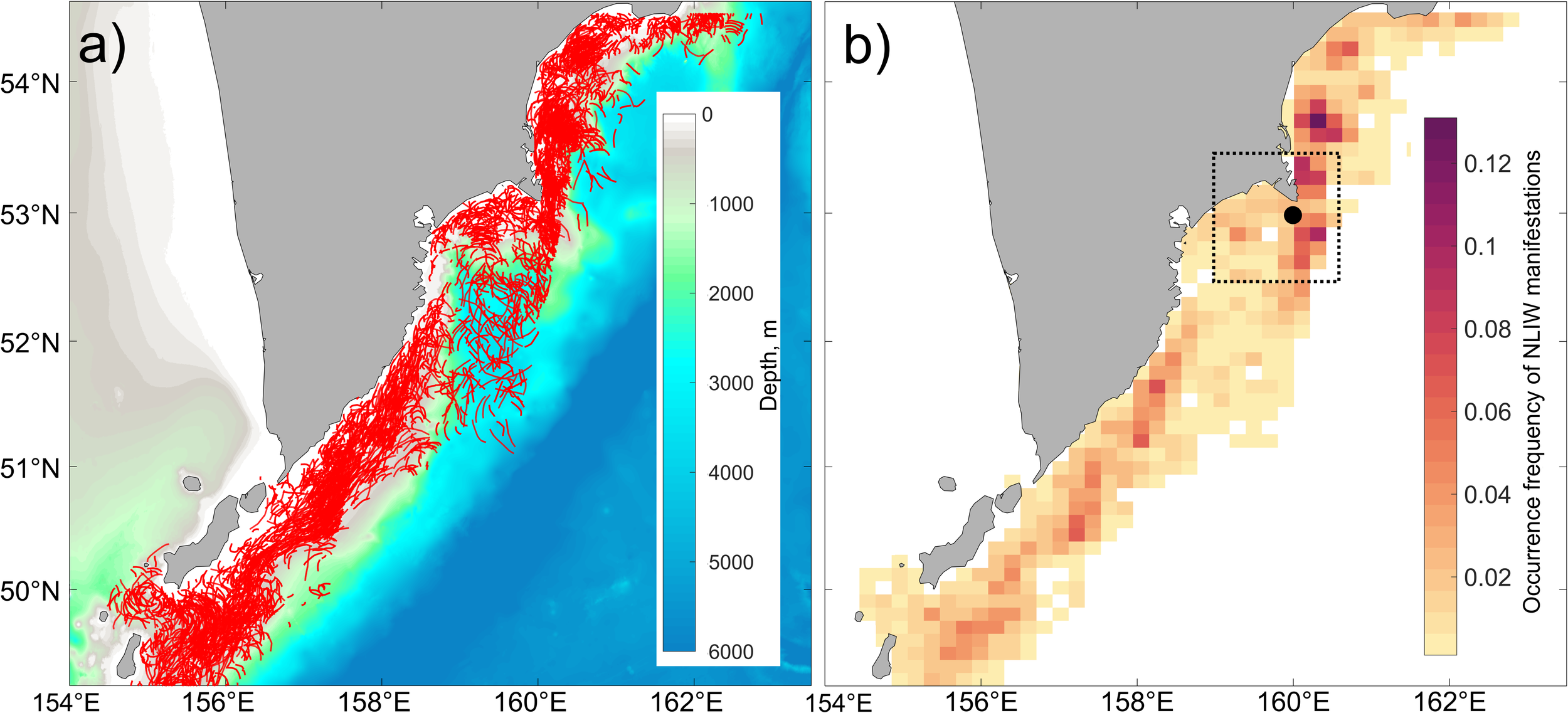
Spatial distribution over the entire period from 2015 to 2024: (a) Locations of leading crests of NLIW manifestations (red curves); (b) Frequency of NLIW occurrence. The black rectangle in panel (b) indicates the “hot spot” area near Cape Shipunsky, and the black circle marks the location where interannual variability of hydrometeorological factors was analyzed.
Data on the interannual variability of detected NLIW manifestations are summarized in Table 1. It should be noted that the distribution of available SAR images across years is uneven: approximately 200 images per year were processed for the study area in 2015–2016, whereas more than 450 images per year were available in 2019–2021. The data show that when the number of available images is low, there is a correlation between data volume and the number of detected wave manifestations. However, once a certain data threshold is reached (over 300 images), this dependence disappears, indicating that such data volume is sufficient for a representative assessment of wave activity for a given year. On average, in years with adequate coverage of SAR images, about 420 NLIW packet manifestations are recorded in the study area annually. The highest ratio of waves per image was observed in 2024 and the lowest in 2020. Despite pronounced interannual fluctuations, there is an overall increasing trend in the number of recorded wave manifestations over the study period.
Table 1
| Year | Number of SAR images, pcs | Number of wave packets, pcs | Avg. number of waves per packet (n), pcs | Avg. wavelength (λ), m | Avg. length of leading crest (cr), km |
|---|---|---|---|---|---|
| 2015 | 182 | 226 | 13 | 351 | 44 |
| 2016 | 194 | 315 | 13 | 332 | 45 |
| 2017 | 368 | 397 | 13 | 322 | 27 |
| 2018 | 398 | 418 | 12 | 335 | 24 |
| 2019 | 445 | 439 | 7 | 433 | 20 |
| 2020 | 466 | 347 | 11 | 362 | 35 |
| 2021 | 452 | 459 | 11 | 397 | 32 |
| 2022 | 321 | 431 | 12 | 282 | 27 |
| 2023 | 327 | 310 | 11 | 345 | 35 |
| 2024 | 338 | 553 | 7 | 373 | 19 |
Annual statistics of NLIW characteristics.
The average number of waves per packet and the length of the leading crests did not exhibit a consistent multi-year trend and showed no pronounced interannual variability (Table 1). Annually both individual wave manifestations (solitons) and large packets containing 35–45 waves (4–5 times greater than the average) were observed. The individual wavelengths varied widely, ranging from 70 to 1500 m. The length of the leading crests of NLIW packets ranged from 2 to 170 km. The mean values of this parameter during the first two years of the study period were 1.5–2 times higher than those in the subsequent eight years, which is likely due to the limited availability of satellite data in the initial years. In years with good SAR data coverage the average crest length was approximately 27 km.
3.2 Seasonal and monthly variability of NLIWs
The seasonal variability of internal wave manifestations can be inferred from Figure 3. The SAR data coverage for each season is substantial with more than 800 images available for the winter and spring seasons and over 900 images for summer and autumn.
Figure 3
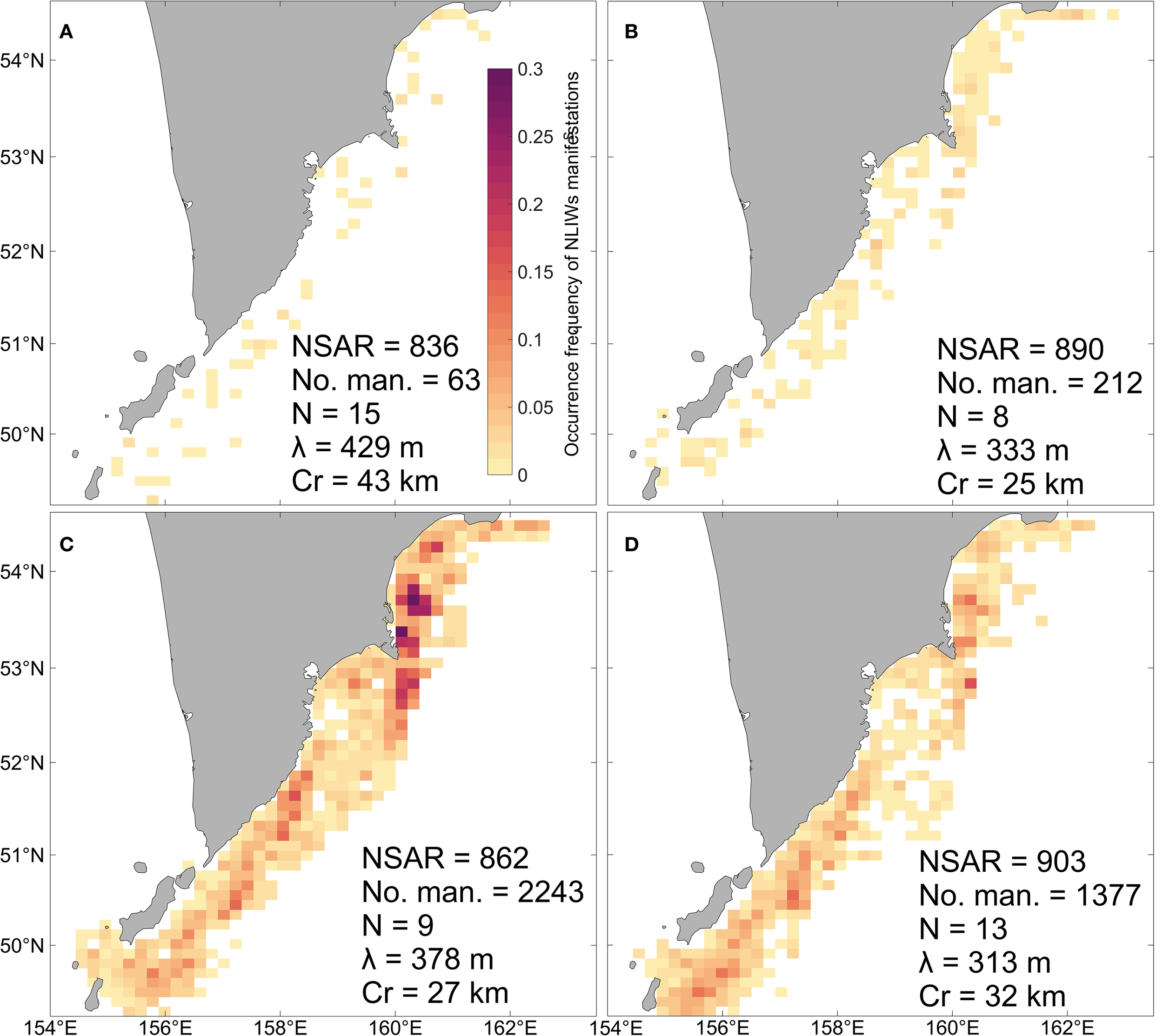
Spatial distribution of NLIW occurrence frequency by multi-year seasonal averages: (A) winter, (B) spring, (C) summer, (D) autumn. NSAR – number of SAR images, NSIWs – number of SAR internal wave manifestations, N – average number of waves in a packet, λ – average wavelength, Cr – average length of the leading crest.
Figure 3A shows that the winter period is characterized by low NLIW occurrence (less than 0.025) across the study region. Isolated, scattered manifestations are primarily recorded along the shelf break and near the continental slope. Overall, the number of waves detected during winter is several times lower than in other seasons. However, the wave packets tend to be more pronounced with the leading crest length averaging over 40 km. These packets also contain a larger number of waves with individual wavelengths exceeding 400 m compared to other seasons.
In the spring period (Figure 3B) the number of detected waves increases by a factor of 3.5 compared to winter, though their geometric dimensions are significantly smaller. The highest occurrence frequencies (0.03–0.04) are observed in the Kronotsky Bay, near the Cape Shipunsky, and in specific areas of the shelf and continental slope off the southeastern Kamchatka Peninsula. In the rest of the region occurrence frequencies remain below 0.025.
During summer (Figure 3C) the number of waves recorded increases by an order of magnitude compared to spring, while the geometric characteristics of the packets remain similar to those in the preceding season. The highest frequencies (exceeding 0.25) are found in the Kronotsky Bay, near the Cape Shipunsky, on the southeastern Kamchatka shelf, and near the Fourth Kuril Strait.
In autumn (Figure 3D) the number of detected waves decreases by half relative to summer. However, packets with larger crest lengths and higher numbers of waves are registered. The maximum occurrence frequency (above 0.12) is observed near the northern Kuril Islands, along the southeastern Kamchatka coast, and near the Cape Shipunsky, where the absolute peak in occurrence is recorded.
Thus, Figure 3 reveals significant seasonal variability in both the frequency and spatial distribution of areas with elevated NLIW occurrences within the study region.
Table 2 presents the intra-annual variability of NLIW occurrences by month. The distribution of SAR images throughout the year is fairly uniform; however, the number of detected waves varies substantially: the minimum values are observed in February, while the maximum (up to 70 times higher) occur in August. Overall, the lowest monthly wave counts (fewer than 21) are recorded from January to March, and the highest—in July and August (over 820). Meanwhile, other wave parameters show less pronounced fluctuations and generally follow the seasonal pattern described above.
Table 2
| Month | Number of SAR images, pcs | Number of wave packets, pcs | Avg. number of waves per packet (n), pcs | Avg. wavelength (λ), m | Avg. length of leading crest (Cr), km |
|---|---|---|---|---|---|
| January | 259 | 20 | 17 | 455 | 51 |
| February | 272 | 14 | 14 | 479 | 40 |
| March | 309 | 21 | 10 | 381 | 33 |
| April | 297 | 69 | 8 | 338 | 27 |
| May | 284 | 122 | 8 | 321 | 22 |
| June | 276 | 385 | 9 | 367 | 28 |
| July | 286 | 866 | 10 | 303 | 30 |
| August | 300 | 992 | 9 | 447 | 24 |
| September | 300 | 824 | 13 | 324 | 30 |
| October | 296 | 453 | 14 | 289 | 35 |
| November | 307 | 100 | 13 | 336 | 32 |
| December | 305 | 29 | 15 | 387 | 39 |
Average characteristics of NLIW occurrences by month.
3.3 Causes of interannual and seasonal variability of NLIWs
In our previous studies (Svergun et al., 2023, 2024), we examined the relationship between high NLIW occurrence in certain years and months and factors that could explain the spatial distribution features of NLIWs. “Hot spots” were identified where more than 50% of all recorded NLIW manifestations were observed. Parameters such as tidal body force (TBF), topographic criticality, and internal Froude number were evaluated, demonstrating the importance of tidal forcing in explaining the causes and features of NLIWs in the region. The results obtained in the present study do not contradict this idea but rather complement it. The stability of these “hot spot” areas both seasonally and interannually supports the hypothesis of their tidal origin.
In the present work we expand our understanding of the variability features of NLIW manifestations for the area best covered by different observational data, which is close to the “hot spot” near Cape Shipunsky (marked by a black rectangle in Figure 2b). A joint analysis was conducted of NLIW variability together with the following factors: (1) upper layer stratification parameters, (2) surface wind speed, and (3) velocities of total tidal currents.
Figure 4 shows the curves of mean values of the above characteristics averaged over 10 years for each month in the “hot spot” near Cape Shipunsky. The shaded corridor indicates the minimum and maximum values of each characteristic per month. Although, as previously noted by Svergun et al. (2024), the masking influence of wind on the number of NLIW manifestations can be significant, the main factors controlling their variability are a combination of favorable hydrological conditions and the strength of tidal forcing. A high multi-year mean occurrence frequency of NLIW manifestations, corresponding to the upper quartile and equal to 1.86, is observed from June to September. This is associated with a multi-year mean density gradient ranging from 0.06 to 0.11 kg/m4, surface mixed layer depth of approximately 10 meters, wind speed between 4 and 8 m/s, and tidal current velocity from 0.22 to 0.26 m/s.
Figure 4
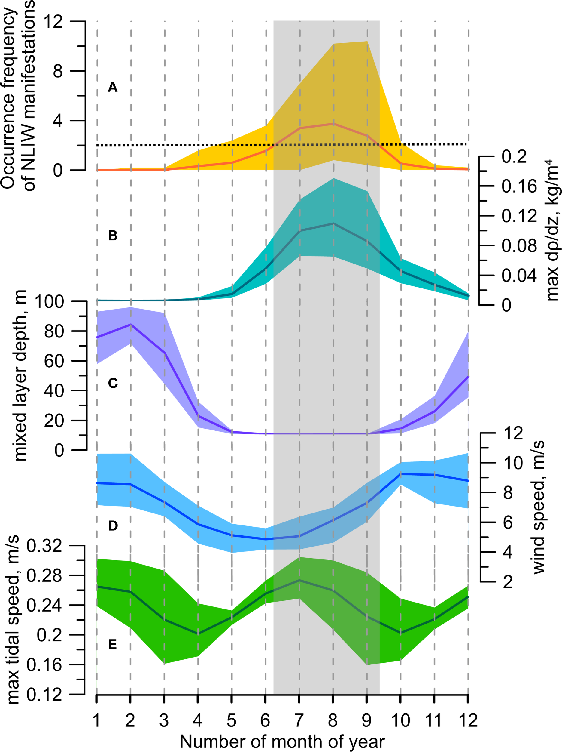
Seasonal variability based on multi-year monthly averages for the “hot spot” near Cape Shipunsky: (A) occurrence frequency of NLIW manifestations; (B) magnitude of maximum vertical density gradient; (C) mixed layer thickness; (D) surface wind speed; (E) maximum total tidal current velocity from the FESOM-C model. The horizontal dashed line in panel (A) indicates the upper quartile of the multi-year mean occurrence frequency of NLIW manifestations. The gray rectangle in panels (B–E) marks the range of variability of hydrometeorological characteristics corresponding to a high occurrence frequency of NLIW manifestations.
Thus, maximum probabilities of NLIW occurrences (defined as the ratio of detected NLIW events to the number of SAR images) occur during the warm months from June to September. During these months we also observe the sharpest pycnocline, minimum thickness of the upper mixed layer, and wind speeds generally below the threshold, above which NLIW detection by SAR dramatically decreases. Additionally, the highest tidal current speeds are observed, whose semiannual modulation in this region is primarily explained by the combination of K1 and P1 tidal harmonics (Svergun et al., 2023).
The pattern of interannual variability and the range of seasonal variability of NLIW manifestations closely coincide with the change in the maximum of density gradient. It is important that this maximum occurs in the pycnocline at the lower boundary of the upper mixed layer formed due to summer heating. Weak density gradient due to autumn-winter convection corresponds with the reduction in the number of surface NLIW manifestations even with high tidal current velocities. Thus, it can be concluded that only a combination of hydrological conditions such as strong subsurface pycnocline, intensified tidal currents and weak winds is linked to the maximum of NLIW occurrences.
3.4 Characteristics of NLIWs from in situ observations
As shown in the previous section, the area near Cape Shipunsky is characterized by high NLIW activity based on SAR data. To verify the correspondence between the characteristics of the detected NLIWs and fluctuations of the near-surface pycnocline (thermocline), results from intensive CTD profiling were used (Figure 5). The temperature records in the 5 to 50 m layer show short-period oscillations with maximum amplitudes observed in the 10 to 20 m layer, where CTD profiling revealed a pronounced seasonal pycnocline with a density gradient of 0.08 kg/m4 coinciding with the thermocline.
Figure 5
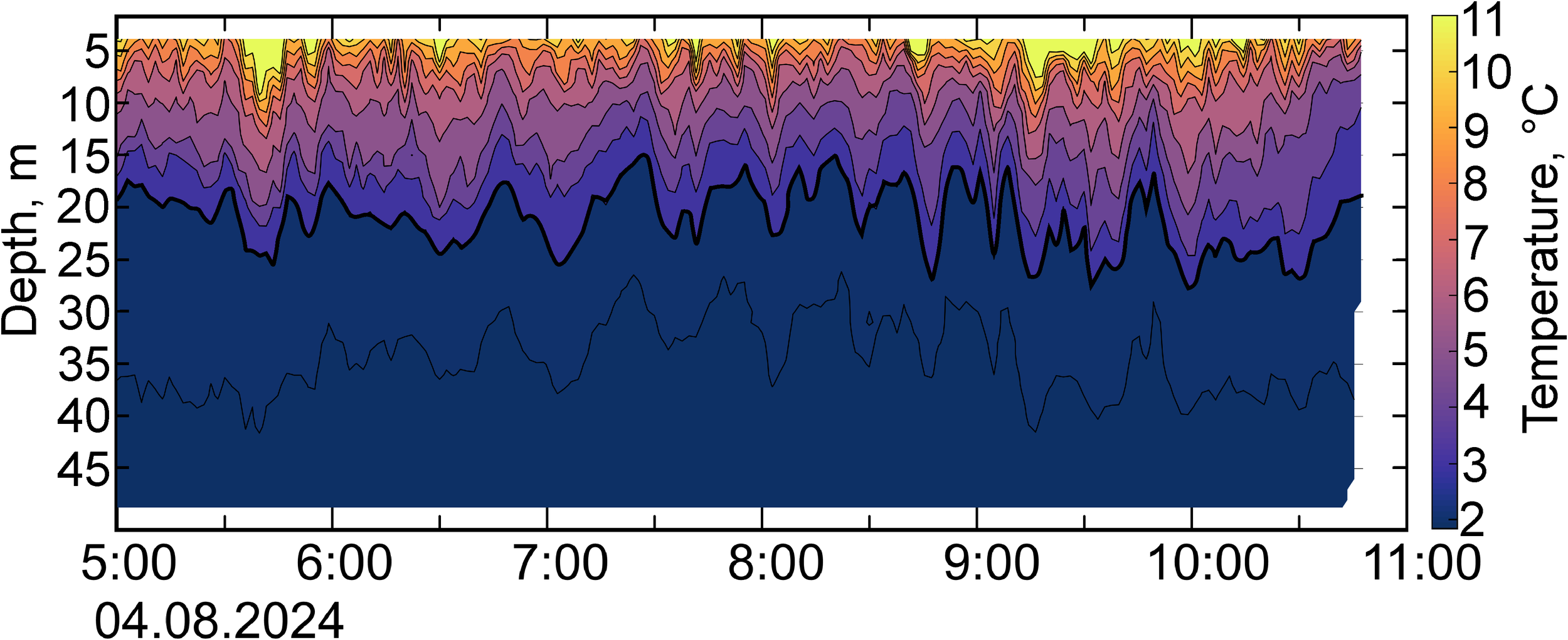
Temperature fluctuation record near Cape Shipunsky based on high-frequency CTD-48M profiler scans. The thick black line indicates the isotherm (2.5°C) corresponding to the lower bound of the pycnocline, which was used for calculating the amplitudes and periods of the NLIWs.
The amplitudes of NLIWs recorded by in situ methods ranged from 0.5 to 3.5 m with an average amplitude of 1.5 m. The NLIW period varied from 6 to 20 minutes. The phase speed was about 0.4 m/s estimated from CTD data (see Section 2.1). Accordingly, the wavelengths as the product of the phase speed and periods ranged from 140 to 480 m and this is consistent with the wavelength range observed in satellite images.
4 Discussion
4.1 Peculiarities of NLIW generation
To verify the validity of the two-layer model dispersion relation for estimating the phase speed of NLIWs, an analysis was performed on the propagation speed of surface manifestations of NLIWs using sequential satellite images. Figure 6 shows the positions of wave fronts superimposed on a bathymetric map along with their propagation directions and the vertical density distribution from in situ data. The phase speed.estimates obtained from tracking the displacement of successive NLIW manifestations closely agrees with one derived from the dispersion relation for two-layer stratification (0.17 m/s from the two-layer dispersion relation versus 0.18 m/s calculated as the ratio of the distance between NLIW manifestations on two consecutive images to the time interval between them). This confirms the adequacy of applying the two-layer approximation in this place. It is noteworthy that based on tidal model data and the observed propagation directions of NLIWs, their formation is likely caused by the interaction of tidal currents with the shelf break. To further test this hypothesis, another example is considered.
Figure 6
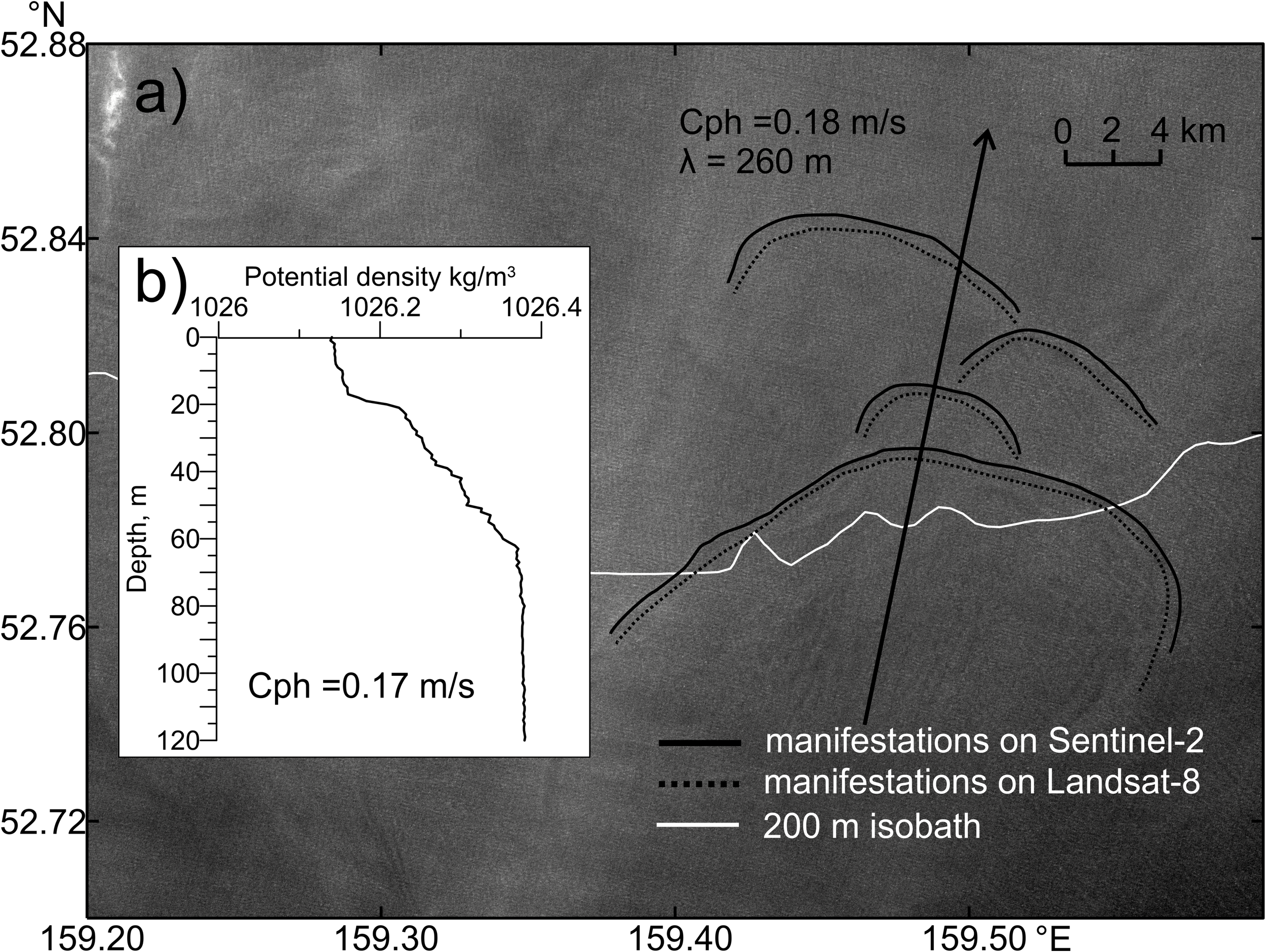
Analysis of NLIWs propagation characteristics based on sequential satellite images: (a) Fragment of the MSI Sentinel-2 green channel image from 25.04.2018 00:26 UTC showing the positions of leading wave crests of NLIW manifestations (solid lines – from MSI Sentinel-2 at 25.04.2018 00:26, dashed lines – from OLI/TIRS Landsat-8 at 25.04.2018 00:16). denotes the phase speed and λ the wavelength estimated from sequential satellite images; (b) Vertical distribution of potential density from in situ measurements taken on 11 April 2018 at the location 52.817°N, 159.02°E (marked with a cross). Here indicates the phase speed estimated using the two-layer approximation.
Figure 7 shows two successive packets of NLIWs, presumably propagating from a single generation source, which we believe, as in the previous case, is located at the shelf break. The distance between the leading crests is 27 km. The vertical distribution of seawater density (panel b), based on reanalysis data in the observed NLIW area, justifies using the dispersion relation for a two-layer stratification to estimate the internal wave propagation speed and thus we get = 0.29 m/s. The period between the two generation events was estimated as the ratio of the distance between the leading crests (25.6 km) to the internal wave speed of 0.29 m/s, yielding approximately 24 hours. This daily period between consecutive NLIW generation events serves as further evidence supporting the tidal generation mechanism.
Figure 7
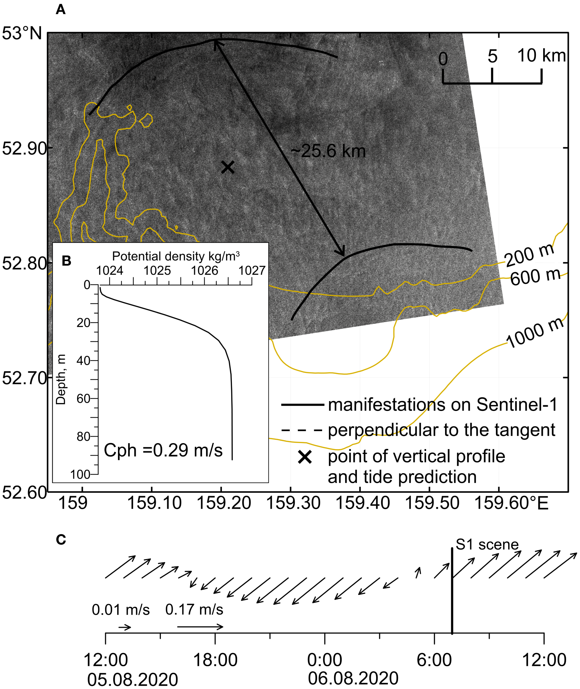
Consecutive manifestations of NLIW packets on a single radar image: (A) fragment of Sentinel-1 image from 06.08.2020 07:17 with marked positions of leading crests of NLIW packets; (B) vertical distribution of potential density from reanalysis data dated 06.08.2020; (C) total tidal currents from the regional FESOM-C model at the same location marked with a cross (the vertical line indicates the time of the satellite image).
Let us focus on the characteristics of tidal currents in the Avacha Bay area, specifically in the “hot spot” near Cape Shipunsky (see Figure 2b), where the individual cases of NLIW manifestations shown in Figures 6 and 7 were examined. Figure 8 presents ellipses of tidal currents for the semidiurnal M2 and diurnal K1 harmonics as well as background currents in the upper layer.
Figure 8
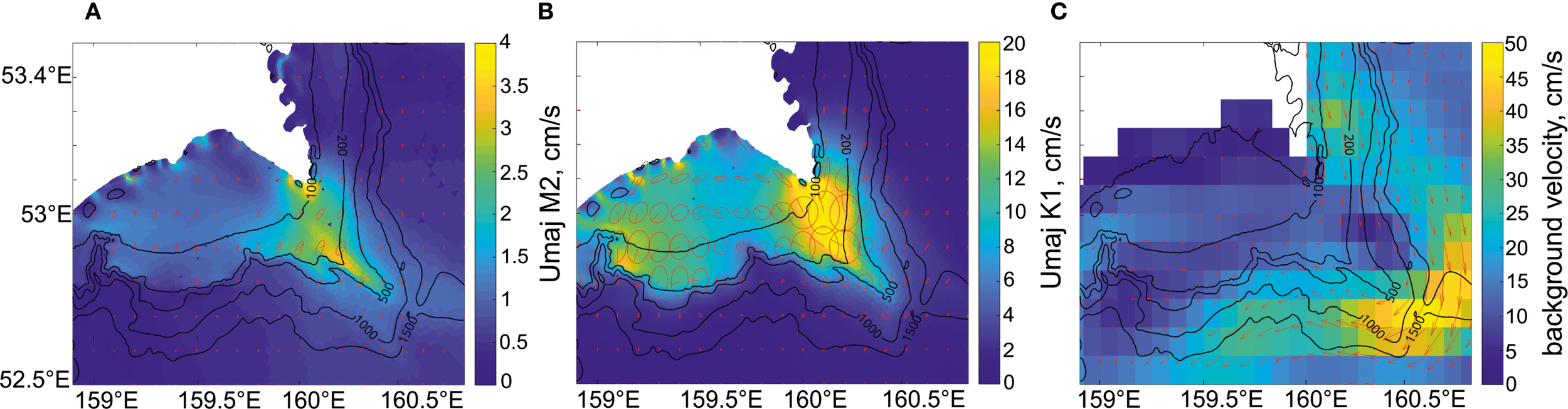
Barotropic tidal current ellipses of principal harmonics (regional model FESOM-C): (A) M2; (B) K1 and (C) mean daily surface currents for 05.08.2020 according to reanalysis data. The amplitude of tidal current velocity (major semiaxis of the tidal ellipse) is represented by color. The ellipses are shown after interpolation of model current characteristics onto a uniform grid. Notice the value of the color scale is different for each of the current maps.
A significant difference between semidiurnal and diurnal tides in the study area is explained by the influence of trapped shelf waves (Romanenkov et al., 2023), which may arise due to intense scattering of the diurnal barotropic tide by coastal and bottom heterogeneities. As shown in Figure 8, the diurnal harmonic currents locally increase near Cape Shipunsky and directly in front of the deep submarine canyon, where they exceed the semidiurnal harmonic currents by an order of magnitude. It should be noted that the area of maximum NLIW occurrence (see Figure 2) corresponds to the area of maximal tidal currents. Considering the tide as a source of internal waves, it should be borne in mind that tides at subinertial frequencies can only generate internal waves that cannot freely propagate away from their generation sites but rather dissipate or break down into NLIW due to nonlinear effects. For the subinertial internal semidiurnal tide at high Arctic latitudes the process of disintegration into high-frequency waves has been confirmed by observations and modeling (Morozov and Paka, 2010; Morozov, 2018). In our case, the diurnal (subinertial) components of the total tidal current prevail over the semidiurnal components; therefore, the topographically trapped internal diurnal tide can be regarded as the source of numerous NLIWs.
In the case presented in Figure 7, the exact moment of NLIW packet generation cannot be determined with certainty. However, we suggest that the most probable timing corresponds to the interval of maximum tidal currents, when their direction aligns with the background flow and the internal Froude number approaches unity. The internal Froude number was estimated as the ratio of the total current speed to the NLIW phase speed: , where , is the magnitude of the tidal current at the time of directional alignment with the background flow within the diurnal cycle, is the magnitude of the background current according to reanalysis data, and is the phase speed of the NLIW. According to Vlasenko et al. (2005), when internal tidal waves undergo transformation and evolve into packets of NLIWs.
4.2 Influence of NLIWs on chlorophyll-a redistribution
A total of 33 instances of banded brightness patterns in the blue and green channels, potentially associated with the redistribution of chlorophyll-a concentrations by propagating NLIWs (Vázquez et al., 2009; Muacho et al., 2013, 2014), were identified across 43 Sentinel-2 images collected between April and August of 2018 and 2024. For these cases, chlorophyll-a concentrations were retrieved using the C2RCC algorithm. An example of chlorophyll-a distribution in an area of frequent NLIW activity near Cape Shipunsky is shown in Figure 9.
Figure 9
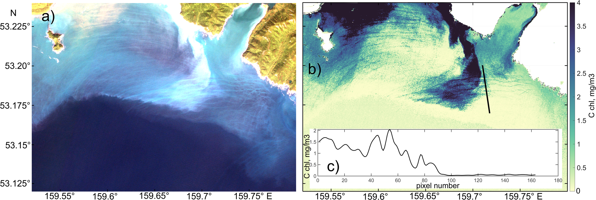
(a) Example of a true-color composite image from MSI Sentinel-2 acquired on 26 August 2024; (b) chlorophyll-a concentration retrieved using the C2RCC algorithm; (c) cross-sectional distribution of chlorophyll-a along the transect indicated in panel (b).
Figure 9a illustrates the presence of suspended matter in the shelf region near Cape Shipunsky, ranging in color from blue-green to white. The scene exhibits distinct banded structures, bright stripes against a darker background, that closely resemble surface manifestation of NLIW packet. The chlorophyll-a retrieval using the C2RCC algorithm (Figure 9b) reveals that concentrations within the high-brightness bands range from 1 to 4 mg/m³. The same banded pattern, attributable to NLIWs and apparent in true-color composites, is also preserved in the chlorophyll-a concentration field. A transect across one such feature shows concentrations varying from 0.5 to 2 mg/m³, while surrounding waters display nearly zero values.
This spatial pattern is typical of nearly all observed cases of brightness banding in the blue and green channels during both spring and summer. The majority of observed NLIW manifestations propagate shoreward and are located over the shelf and continental slope. Thus, this example demonstrates that in “hot spots” NLIWs propagating onto the shelf may play a significant role in redistributing phytoplankton biomass.
Given that August is the month of peak NLIW activity (see Table 2), we analyzed the interannual variability of chlorophyll-a concentration and NLIW occurrence frequency in the “hot spot” region near Cape Shipunsky. The analysis covered Augusts from 2017 to 2024 (see Figure 10).
Figure 10
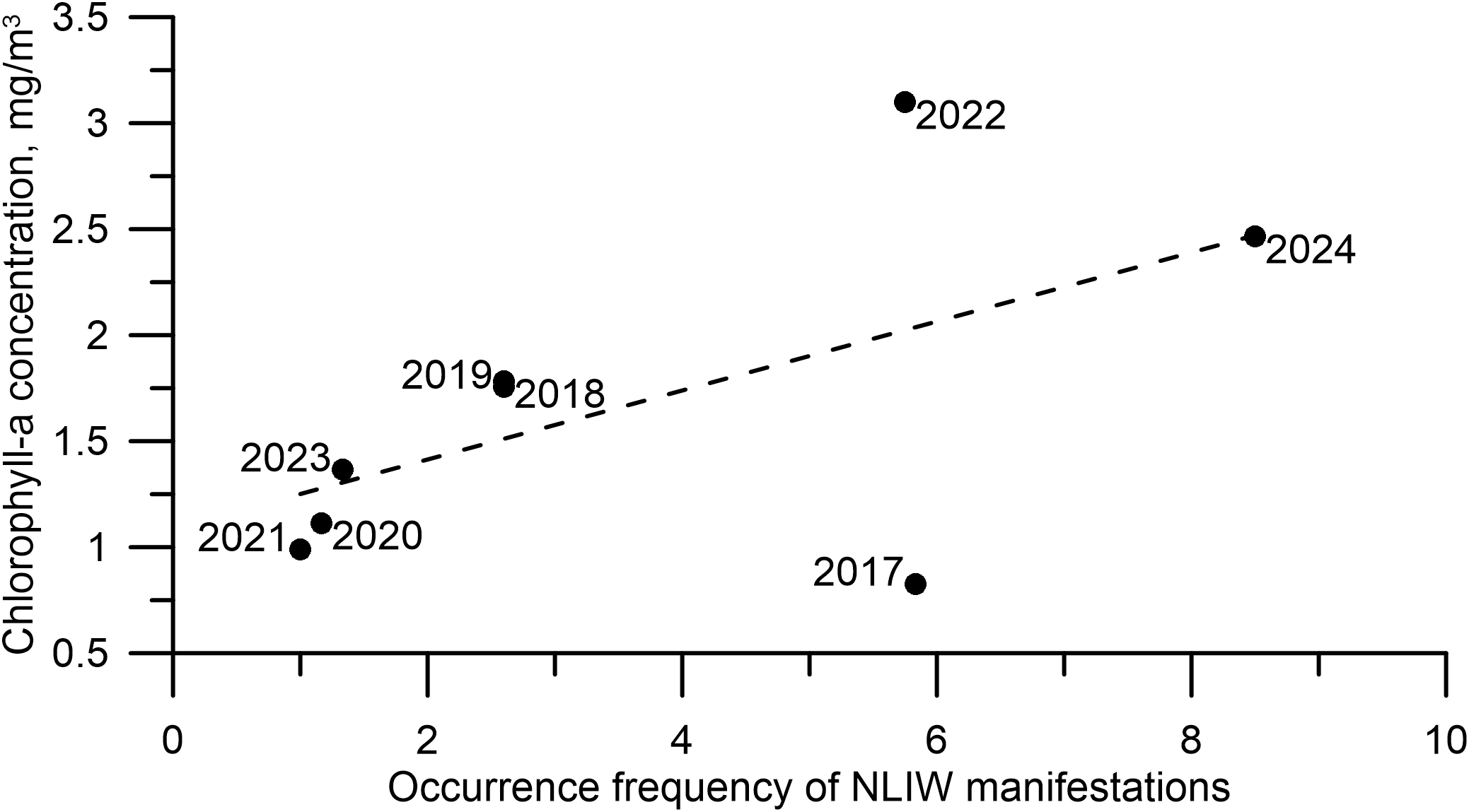
Variability of chlorophyll-a concentration (MODIS data) and frequency of NLIW occurrences in the “hot spot” region near Cape Shipunsky during Augusts from 2017 to 2024. The dashed line shows the linear approximation of the relationship between the described variables with R² (coefficient of determination) equal to 0.4.
In general, the lowest frequencies of NLIW occurrences correspond to the lowest chlorophyll-a concentrations, while the highest frequencies align with peak concentrations. However, a notable area stands out where moderately high NLIW occurrence frequencies are associated with both low and high chlorophyll-a concentrations. Despite this scatter, the relationship between chlorophyll-a concentration and NLIW frequency can be roughly approximated by a linear trend, though with some caveats. This suggests that multiple factors likely influence chlorophyll-a variability. Nonetheless, the frequent appearance of NLIW-like surface patterns in regions of enhanced green-channel brightness in optical satellite imagery supports the potential existence of such a relationship.
It is well established that food availability during the transition of fish larvae to exogenous feeding plays a critical role in determining fish cohort recruitment success. This issue, as it pertains to walleye pollock in the Sea of Okhotsk, was addressed to some extent by Gorbatenko et al. (2004) and Maksymenkov (2007). The diet of larval and post larval stages is not particularly diverse with both the composition and size of consumed prey strongly dependent on larval size. Phytoplankton generally serves as a food source only at the very onset of exogenous feeding (Kamba, 1977; Maksymenkov, 1984; Nishiyama et al., 1986). However, in certain regions—such as the Korea Bay and the Pacific waters off Kamchatka Peninsula — phytoplankton plays a significant role in the diet from the earliest larval stages.
As larvae grow, smaller prey items are progressively replaced by larger ones. In many areas nauplii of copepods dominate the diet of larvae up to 14 mm in length. In some locations eggs of copepods and euphausiids are also commonly consumed by smaller larvae. With increasing size the larval diet becomes more diverse. By 6–8 mm length early copepodite stages, as well as small copepods such as Oithona similis, Pseudocalanus minutus, Acartia longiremis, and others, begin to appear in the diet. From 14 mm onwards Pseudocalanus minutus becomes the dominant prey item. The role of this species—across both early developmental stages and adults—is exceptional in the diet of pollock larvae. Pseudocalanus minutus typically constitutes a major portion of the plankton community, both as nauplii and copepodites, and in most cases determines the condition of the larval feeding base for pollock (Shuntov et al., 1993).
Abundance and availability of planktonic prey are not always the primary factors ensuring high survival of fish larvae (Drinkwater and Myers, 1987; Gaard, 1999; Sundby, 2000). Of particular importance for larval survival are the early-summer formation of subsurface “growth layers”, where large aggregations of walleye pollock larvae are often observed. If these layers contain sufficient concentrations of accessible prey, they may significantly enhance larval survival.
Given the potential role of NLIWs in delivering nutrients to shelf waters that stimulate phytoplankton growth, we examined the abundance of 2-year-old pollock and the frequency of NLIW manifestations over the period May–September. In Figure 11 lowest frequencies of NLIW occurrences correspond to the lowest abundance of 2-year-old walleye pollock with a two-year lag, while the highest frequencies align with peak abundance with a two-year lag. However, this trend is not observed in 2019/2017 and 2023/2021. A joint interpretation of Figures 9 and 10 suggests that NLIWs may play a role in regulating the abundance of ichthyoplankton and early fish life stages. Clearly, further testing of this hypothesis will require new targeted observational evidence.
Figure 11
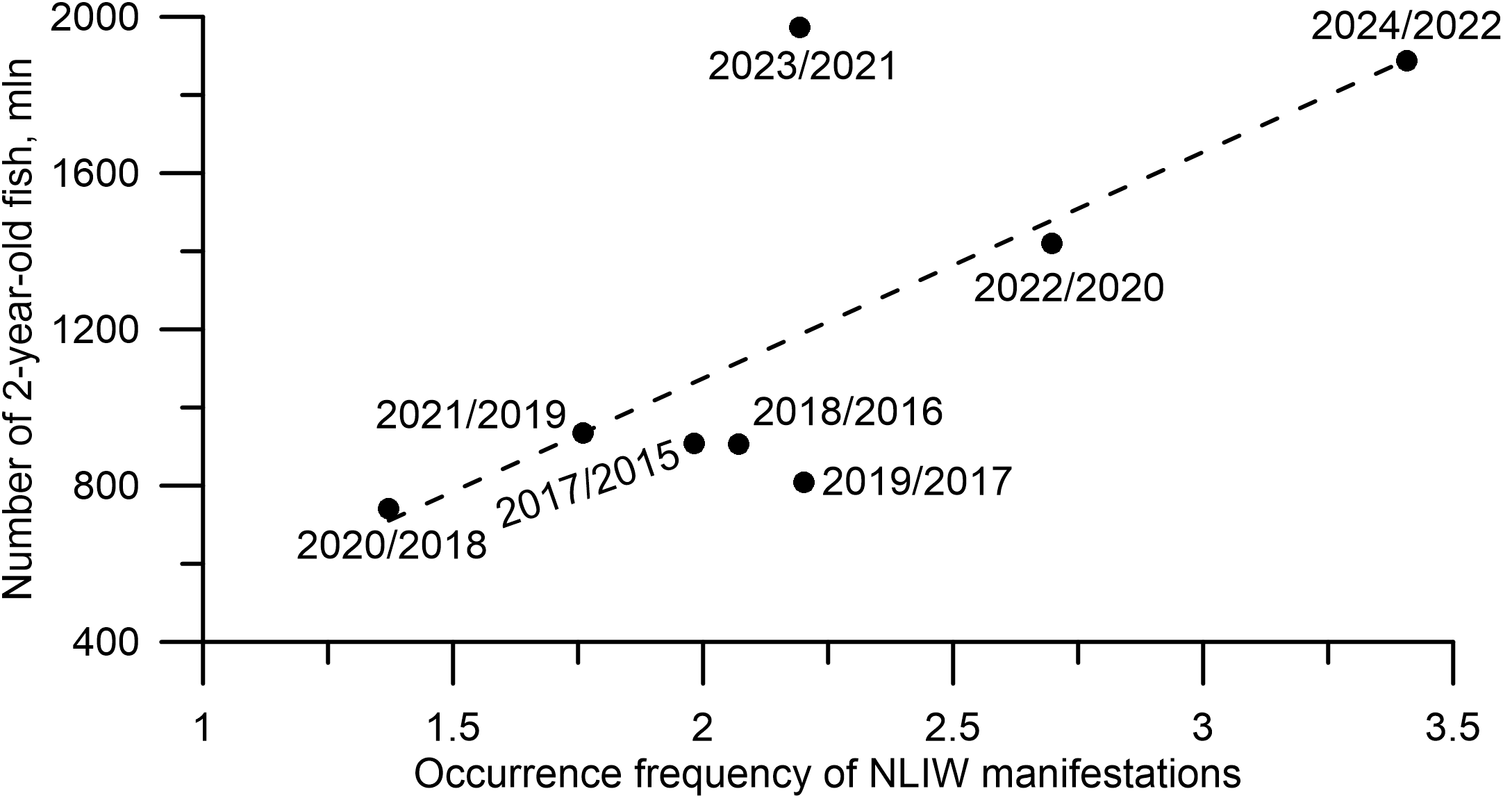
Interannual variability in the abundance of 2-year-old walleye pollock and the frequency of observed NLIW manifestations from May to September during 2017/2015–2024/2022. The dashed line shows the linear approximation of the relationship between the described variables with R² (coefficient of determination) equal to 0.6.
5 Conclusions
The analysis of radar satellite imagery from 2015 to 2024 enabled the detection of approximately 4,000 NLIW manifestations in the Pacific Ocean off the Kamchatka Peninsula and the northern Kuril Islands. NLIW packets were observed nearly continuously across the shelf, continental slope, and deepwater parts of the Avacha Bay. Based on the frequency of NLIW occurrences, several “hot spot” regions were identified east of the Fourth Kuril Strait, over the southeastern Kamchatka shelf, and around the Shipunsky Peninsula, and in the Kronotsky Bay. The highest frequency and number of NLIW manifestations across all “hot spots” occur during the summer season.
The interannual stability of these “hot spots” areas, supported by several illustrative cases, confirms the previously proposed hypothesis of their tidal origin, notably involving diurnal tidal components—an atypical feature for most regions of the World Ocean. Statistically robust estimates of the intra-seasonal variability of NLIW characteristics were obtained. Notably, despite seasonal fluctuations, the geometric properties of NLIW packets remained stable on interannual timescales. Using the “hot spot” near the Shipunsky Peninsula as a case study, we demonstrated that the annual number of observed NLIW events is modulated by the presence of a strong subsurface pycnocline, tidal current strength, and wind forcing.
In turn, increased NLIWs activity over the shelf enhances phytoplankton development—and consequently ichthyoplankton survival—through mixing of the surface layer and upward transport of nutrients from deeper layers. These findings suggest a local contribution of NLIWs to shaping the productivity of the oceanic surface layer. It is worth emphasizing that environmental drivers operating on such short timescales are often overlooked as conventional approaches in fisheries oceanography and ichthyology tend to focus on population dynamics and environmental variability at seasonal and interannual scales.
A promising direction for future research is the development of a regional tidal model that incorporates the complex nonlinear and baroclinic dynamics responsible for observed NLIWs clustering in “hot spots”, along with targeted multidisciplinary (hydrological and ichthyological) field campaigns in these areas.
Statements
Data availability statement
The original contributions presented in the study are included in the article/Supplementary Material. Further inquiries can be directed to the corresponding author.
Author contributions
AZ: Supervision, Writing – original draft, Writing – review & editing, Funding acquisition, Data curation, Formal analysis, Conceptualization, Methodology. ESv: Supervision, Formal analysis, Visualization, Funding acquisition, Data curation, Software, Writing – original draft, Conceptualization, Methodology, Writing – review & editing, Validation. ESo: Data curation, Writing – original draft, Formal analysis, Visualization, Methodology, Software, Funding acquisition, Conceptualization, Writing – review & editing. DR: Formal analysis, Writing – original draft, Funding acquisition, Software, Methodology, Data curation, Writing – review & editing. AV: Validation, Data curation, Writing – review & editing, Formal analysis, Writing – original draft, Funding acquisition. AK: Software, Funding acquisition, Writing – review & editing, Formal analysis, Writing – original draft, Data curation. OA: Writing – review & editing, Data curation, Software, Funding acquisition, Validation. AM: Validation, Writing – original draft, Data curation. IV: Writing – original draft, Validation, Data curation.
Funding
The author(s) declare financial support was received for the research and/or publication of this article. This research was supported by the Russian Science Foundation, project no. 23-17-00174 (https://rscf.ru/en/project/23-17-00174/).
Acknowledgments
The authors express their gratitude to the research team of the 2004 Pacific Floating University program aboard the R/V Professor Multanovskiy, during which in situ observations of NLIWs were conducted as part of the All-Russian Research and Educational Program “Floating University” (Agreement No. 075-03-2024-117). The authors are grateful to Ekaterina S. Kochetkova for her help in editing English text of the manuscript.
Conflict of interest
The authors declare that the research was conducted in the absence of any commercial or financial relationships that could be construed as a potential conflict of interest.
Generative AI statement
The author(s) declare that no Generative AI was used in the creation of this manuscript.
Any alternative text (alt text) provided alongside figures in this article has been generated by Frontiers with the support of artificial intelligence and reasonable efforts have been made to ensure accuracy, including review by the authors wherever possible. If you identify any issues, please contact us.
Publisher’s note
All claims expressed in this article are solely those of the authors and do not necessarily represent those of their affiliated organizations, or those of the publisher, the editors and the reviewers. Any product that may be evaluated in this article, or claim that may be made by its manufacturer, is not guaranteed or endorsed by the publisher.
Supplementary material
The Supplementary Material for this article can be found online at: https://www.frontiersin.org/articles/10.3389/fmars.2025.1662937/full#supplementary-material
References
1
Alpers W. (1985). Theory of radar imaging of internal waves. Nature314, 245–247. doi: 10.1038/314245a0
2
Andreev A. Pipko I. (2022). Water circulation, temperature, salinity, and pCO2 distribution in the surface layer of the east kamchatka current. J. Mar. Sci. Eng.10, 1787. doi: 10.3390/jmse10111787
3
Bondur V. G. Serebryany A. N. Zamshin V. V. (2020). Registering fish shoals attracted by solitary intensive internal waves. Dokl. Earth Sci.492, 471–474. doi: 10.1134/S1028334X20060033
4
Buslov A. V. (2008). Walleye pollock of the eastern Kamchatka coast: modern state of stock and recommendations for rational exploitation. Izvestiya. TINRO.152, 3–17.
5
Drinkwater K. F. Myers R. A. (1987). Testing predictions of marine fish and shellfish landings from environmental variables. Can. J. Fish. Aquat. Sci.44, 1568–1573. doi: 10.1139/f87-189
6
Embling C. B. Sharples J. Armstrong E. Palmer M. R. Scott B. E. (2013). Fish behavior in response to tidal variability and internal waves over a shelf sea bank. Prog. Oceanogr.117, 106–117. doi: 10.1016/j.pocean.2013.06.013
7
Etkin V. S. Srnirnov A. V. (1992). “ Observations of internal waves in ocean by radar methods,” in (Proceedings) IGARSS’92 International Geoscience and Remote Sensing Symposium, International Space Year: Space Remote Sensing, Vol. 1. 143–145 (Hamburg: IEEE). doi: 10.1109/IGARSS.1992.576651
8
Ezer T. Heyman W. D. Houser C. Kjerfve B. (2010). Modeling and observations of high-frequency flow variability and internal waves at a Caribbean reef spawning aggregation site. Ocean. Dyn.61, 581–598. doi: 10.1007/s10236-010-0367-2
9
Gaard E. (1999). The zooplankton community structure in relation to its biological and physical environment on the Faroe shelf 1989-1997. J. Plankton. Res.21, 1133–1152. doi: 10.1093/plankt/21.6.1133
10
Garwood J. C. Musgrave R. C. Lucas A. J. (2020). Life in internal waves. Oceanography33, 38–49. doi: 10.5670/oceanog.2020.313
11
Gorbatenko K. M. Merzylyakov A. Shershenkov S. (2004). Feeding patterns in different size larvae of walleye pollack, Theragra chalcogramma (Pallas 1814) on the shelf of western Kamchatka. Russian J. Mar. Biol.30, 113–120. doi: 10.1023/B:RUMB.0000025987.11438.72
12
Greer A. T. Cowen R. K. Guigand C. M. Hare J. A. Tang D. (2014). The role of internal waves in larval fish interactions with potential predators and prey. Prog. Oceanogr.127, 47–61. doi: 10.1016/j.pocean.2014.05.010
13
Guan Z. Ge R. Li Y. Zou L. Yang S. (2023). Diel variation of phytoplankton communities in the northern south China sea under the effect of internal solitary waves and its response to environmental factors. Water15, 2422. doi: 10.3390/w15132422
14
Helfrich K. R. Melville W. K. (2006). Long nonlinear internal waves. Annu. Rev. Fluid. Mech.38, 395–425. doi: 10.1146/annurev.fluid.38.050304.092129
15
Ilin O. I. (2022). On application of Kalman filters in cohort models. Izv. Tikhookean. Nauchno-Issled. Inst. Rybn. Khoz. Okeanogr.202, 601–622. doi: 10.26428/1606-9919-2022-202-601-622
16
Itoh S. Tanaka Y. Osafune S. Yasuda I. Yagi M. Kaneko H. et al . (2014). Direct breaking of large-amplitude internal waves in the Urup Strait. Prog. Oceanogr.126, 109–120. doi: 10.1016/j.pocean.2014.04.014
17
Jackson C. R. (2004). An Atlas of Internal Solitary-like Waves and their Properties (Alexandria: Global Ocean Associates), 560. Available online at: https://www.internalwaveatlas.com/Atlas2_index.html.
18
Jones N. L. Ivey G. N. Rayson M. D. Kelly S. M. (2020). Mixing driven by breaking nonlinear internal waves. Geophys. Res. Lett.47, e2020GL089591. doi: 10.1029/2020GL089591
19
Kamba M. (1977). Feeding habits and vertical distribution of walleye pollock, Theragra chalcogramma, (Pallas) in early life stage in Uchiura Bay, Hokkaido. Res. Inst. N. Pac. Fish. Hokkaido. Univ., 175–197.
20
Konik A. A. Zimin A. V. Atadzhanova O. A. Svergun E. I. Romanenkov D. A. Sofina E. V. et al . (2024). Intra-day variability of vertical water structure and distributions walleye pollock eggs in the deep-sea canyons of avacha bay: A field experiment during the spawning period. Fundam. Appl. Hydrophys.17, 77–89. doi: 10.59887/2073-6673.2024.17(4)-6
21
Konyaev K. V. Sabinin K. D. (1992). Volny vnutri okeana (Leningrad: Gidrometeoizdat), 272.
22
Kozlov I. E. Atadzhanova O. A. Zimin A. V. (2022). Internal solitary waves in the white sea: hot-spots, structure, and kinematics from multi-sensor observations. Remote Sens.14, 4948. doi: 10.3390/rs14194948
23
Lavrova O. Y. Sabinin K. D. Badulin S. I. (1999). “ Radar observation of internal wave and current interactions,” in Proceedings of the 1999 IEEE International Geoscience and Remote Sensing Symposium (IGARSS'99) 'Remote Sensing of the Systems Earth - A Challenge for the 21st Century' (Hamburg: Institute of Electrical and Electronics Engineers), Vol. 1. 159–161. doi: 10.1109/IGARSS.1999.773433
24
Lucas A. J. Pinkel R. (2020). Observations of coherent transverse wakes in shoaling nonlinear internal waves. J. Phys. Oceanogr.52, 1277–1293. doi: 10.1175/JPO-D-21-0059.1
25
Ma L. Bai X. Laws E. A. Xiao W. Guo C. Liu X. et al . (2023). Responses of phytoplankton communities to internal waves in oligotrophic oceans. J. Geophys. Res.: Oceans.128, e2023JC020201. doi: 10.1029/2023JC020201
26
Maksymenkov V. V. (1984). Pishhevye otnoshenija lichinok nekotoryh ryb v zal. Korfa. Voprosy ihtiologii24, 972–978.
27
Maksymenkov V. V. (2007). Nutrition and food relationships of young fish living in river estuaries and coastal areas of Kamchatka (Petropavlovsk-Kamchatskij: KamchatNIRO), 278.
28
McBride K. MacKinnon J. Franks P. J. S. McSweeney J. M. Waterhouse A. F. Palóczy A. et al . (2024). A juvenile journey: Using a highly resolved 3D mooring array to investigate the roles of wind and internal tide forcing in across-shore larval transport. Limnol. Oceanogr.69, 2364–2376. doi: 10.1002/lno.12675
29
Morozov E. G. (2018). Oceanic Internal Tides: Observations, Analysis and Modeling: A Global View (Berlin: Springer), 304. doi: 10.1007/978-3-319-73159-9
30
Morozov E. G. Paka V. T. (2010). Internal waves in a high latitude region. Oceanology50, 668–674, 5. doi: 10.1134/S0001437010050048
31
Muacho S. da Silva J. C. B. Brotas V. Oliveira P. B. Magalhaes J. M. (2014). Chlorophyll enhancement in the central region of the Bay of Biscay as a result of internal tidal wave interaction. J. Mar. Syst.136, 22–30. doi: 10.1016/j.jmarsys.2014.03.016
32
Muacho S. Silva J. C. Brotas V. Oliveira P. B. (2013). Effect of internal waves on near-surface chlorophyll concentration and primary production in the Nazaré Canyon (west of the Iberian Peninsula). Deep. Sea. Res. Part I.: Oceanograph. Res. Papers.81, 89–96. doi: 10.1016/j.dsr.2013.07.012
33
Navrotsky V. V. Pavlova E. P. Liapidevskii V. (2012). Internal waves and their biological effects in the shelf zone of sea. Vestnik. Far. Eastern. Branch. Russian Acad. Sci.6, 22–31.
34
Nishino S. Kawaguchi Y. Inoue J. Hirawake T. Fujiwara A. Futsuki R. et al . (2015). Nutrient supply and biological response to wind-induced mixing, inertial motion, internal waves, and currents in the northern Chukchi Sea. J. Geophys. Res.: Oceans.120, 1975–1992. doi: 10.1002/2014JC010407
35
Nishiyama Т. Hirano К. Haryn T. (1986). The early life history and feeding habits of larval walleye pollock Theragra chalcogramma (Pallas) in the southeast Bering Sea. Bull. INPFC.45, 177–227.
36
Pao H. P. He Q. (2002). Generation and Transformation of Intense Internal Waves on Shelves (Washington: The University of Maryland, COAA Scientific Workshop, Collage Park).
37
Pao H. P. Serebryany A. N. (2005). “ Studies of intense internal gravity waves: field measurements and numerical modeling,” in Advances in Engineering Mechanics Reflections and Outlooks: In Honor of Theodore T-Y Wu. Eds. ChuangA. T.TengM. H.ValentineD. T., (Moscow: World Scientific Publishing Co.) 286–296. doi: 10.1142/9789812702128_0021
38
Reid E. C. DeCarlo T. M. Cohen A. L. Wong G. T. Lentz S. J. Safaie A. et al . (2019). Internal waves influence the thermal and nutrient environment on a shallow coral reef. Limnol. Oceanogr. Lett.64, 1949–1965. doi: 10.1002/lno.11162
39
Robinson I. S. (2010). “ Internal waves,” in Discovering the Ocean from Space. Springer Praxis Books ( Springer, Berlin, Heidelberg), 453–483. doi: 10.1007/978-3-540-68322-3_12
40
Romanenkov D. A. Sofina E. V. Rodikova A. E. (2023). Modeling of Barotropic tide off the southeastern coast of the kamchatka peninsula in view of the accuracy of global tidal models in the northwest pacific ocean. Fundam. Appl. Hydrophys.16, 45–62. doi: 10.59887/2073-6673.2023.16(4)-4
41
Sabinin K. D. Serebryany A. N. (2007). Hot spots” in the field of internal waves in the ocean. Acoust. Phys.53, 357–380. doi: 10.1134/S1063771007030128
42
Serebryany A. N. (2000). “ Internal waves on Pacific shelf of Kamchatka (Preliminary results of internal wave field observations),” in Proceedings of the US-Russia workshop on experimental acoustics. Ed. TalanovV. I. ( Institute of Applied Physics, Nizhny Novgorod), 116–122.
43
Shcherbakova V. S. Rouvinskaya E. A. Kurkina O. E. (2024). Numerical modeling and analysis of spatiotemporal features of the field of internal waves in Avacha bay. Ecol. Syst. Devices.9, 44–56. doi: 10.25791/esip.9.2024.1474
44
Shevchenko G. V. Chastikov V. N. Ulchenko V. A. (2025). Features of hydrological regime nearby the pacific coast of the northern kuril islands based on ship oceanographic surveys. Phys. Oceanogr.32, 253–269.
45
Shroyer E. L. Moum J. N. Nash J. D. (2010). Vertical heat flux and lateral mass transport in nonlinear internal waves. Geophys. Res. Lett.37, L08601. doi: 10.1029/2010GL042715
46
Shuntov V. Volkov A. Temnyka O. Dylepova E. (1993). Pollock in the ecosystems of the far-eastern seas (Vladivostok: Pacific Institute of Fisheries and Oceanology), 426.
47
Sundby S. (2000). Recruitment of Atlantic cod stocks in relation to temperature and advectlon of copepod populations. Sarsia85, 277–298. doi: 10.1080/00364827.2000.10414580
48
Svergun E. I. Sofina E. V. Zimin A. V. Kruglova K. A. (2023). Seasonal variability of characteristics of nonlinear internal waves in the Kuril-Kamchatka region by Sentinel 1 data. Cont. Shelf. Res.259, 104986. doi: 10.1016/j.csr.2023.104986
49
Svergun E. I. Zimin A. V. (2020). Characteristics of short-period internal waves in the avacha bay based on the in situ and satellite observations in August-September 2018. Phys. Oceanogr.27, 278–289. doi: 10.22449/1573-160X-2020-3-278-289
50
Svergun E. I. Zimin A. V. Konik A. A. (2024). Short-period internal waves in the pacific area of the Kamchatka peninsula and the northern Kuril Islands according to 2017–2021 satellite radar observations. Sovremennye. Problemy. Distancionnogo. Zondirovanija. Zemli. iz Kosmosa.21, 251–260. doi: 10.21046/2070-7401-2024-21-2-251-260
51
Varkentin A. I. Saushkina D. Y. (2022). On some issues of pollock reproduction in the Pacific waters adjacent to Kamchatka and the Northern Kuril Islands in 2013-2022. Trudy. VNIRO.189, 105–119. doi: 10.36038/2307-3497-2022-189-105-119
52
Varkentin A. I. Tepnin O. B. Saushkina D. Zimin A. V. Svergun E. I. (2024). “ The yield of generations of East Kamchatka pollock and some of the reasons for it,” in Conservation of the biodiversity of Kamchatka and adjacent seas: Proceedings of the XV All-Russian Scientific Conference dedicated to the 130th anniversary of the birth of the outstanding Russian researcher of the ichthyofauna of the Far East, Petropavlovsk-Kamchatsky, Moskow, November 14-15, 2024. 400 ( Publishing House of the Wildlife Conservation Center). doi: 10.53657/KBPGI041.2024.43.18.035
53
Vázquez A. Flecha S. Bruno M. Macias D. Navarro G. (2009). Internal waves and short-scale distribution patterns of chlorophyll in the Strait of Gibraltar and Alborán Sea. Geophys. Res. Lett.36, 23. doi: 10.1029/2009GL040959
54
Villamaña M. Mouriño-Carballido B. Marañón E. Cermeño P. Chouciño P. da Silva J. C. B. et al . (2017). Role of internal waves on mixing, nutrient supply and phytoplankton community structure during spring and neap tides in the upwelling ecosystem of Ría de Vigo (NW Iberian Peninsula). Limnol. Oceanogr. Lett.62, 1014–1030. doi: 10.1002/lno.10482
55
Vlasenko V. Stashchuk N. Hutter K. (2005). Baroclinic Tides: Theoretical Modeling and Observational Evidence (Cambridge: Cambridge University Press), 351. doi: 10.1017/CBO9780511535932
56
Zimin A. V. Romanenkov D. A. Konik A. A. Atadzhanova O. A. Svergun E. I. Varkentin A. I. et al . (2024). Multiscale Eddies dynamics in the pacific ocean adjacent to the kamchatka peninsula and the northern kuril islands. Ecol. Saf. Coast. Shelf. Zones. Sea.3, 16–35.
Summary
Keywords
internal waves, Sentinel-1, ocean tides, FESOM-C model, CTD profiling, chlorophyll-a, fishery resources, northern Pacific Ocean
Citation
Zimin A, Svergun E, Sofina E, Romanenkov D, Varkentin A, Konik A, Atadzhanova O, Makhovikov A and Vinogradova I (2025) Interannual variability of nonlinear internal wave characteristics in the Pacific Ocean off the Kamchatka Peninsula and the Northern Kuril Islands. Front. Mar. Sci. 12:1662937. doi: 10.3389/fmars.2025.1662937
Received
09 July 2025
Accepted
09 September 2025
Published
26 September 2025
Volume
12 - 2025
Edited by
Jing Yu, Chinese Academy of Fishery Sciences (CAFS), China
Reviewed by
Nancy Soontiens, Fisheries and Oceans Canada (DFO), Canada; Kumar Ravi Prakash, Indian Institute of Technology Delhi, India
Updates
Copyright
© 2025 Zimin, Svergun, Sofina, Romanenkov, Varkentin, Konik, Atadzhanova, Makhovikov and Vinogradova.
This is an open-access article distributed under the terms of the Creative Commons Attribution License (CC BY). The use, distribution or reproduction in other forums is permitted, provided the original author(s) and the copyright owner(s) are credited and that the original publication in this journal is cited, in accordance with accepted academic practice. No use, distribution or reproduction is permitted which does not comply with these terms.
*Correspondence: Alexey Zimin, zimin2@mail.ru
Disclaimer
All claims expressed in this article are solely those of the authors and do not necessarily represent those of their affiliated organizations, or those of the publisher, the editors and the reviewers. Any product that may be evaluated in this article or claim that may be made by its manufacturer is not guaranteed or endorsed by the publisher.