The impact of submesoscale frontogenesis on microscale turbulence in the Tsushima Warm Current

The process of submesoscale frontogenesis within the Tsushima Warm Current (TWC) front, and the enhancement of the microscale turbulence associated with this frontogenesis, was examined using in situ observational data. Multiple sections across the front captured deformation flow on the western side of the southward-flowing meander crest from the main axis of the TWC front. The frontogenesis was caused by deformation within the observed area. Submesoscale patches encompassing different water masses were found near the growing front. Observation of microstructure revealed that the turbulent dissipation rates and the vertical diffusivity were relatively large near the area of strong deformation flow and patchy structure. This turbulence is attributed to frontogenesis and the patchy pattern of the water mass. The estimation of the vertical buoyancy flux and the resulted energy conversion revealed that only a few percent of the energy supplied by the ageostrophic secondary circulation needs to cascade into turbulence to account for the observed turbulent dissipation. The results indicate that the submesoscale frontogenesis and the resulting submesoscale water mass patterns, which are ubiquitous over the global ocean, contribute to the turbulent mixing and consequently to the effective energy cascade.

1 Introduction

Oceanic frontogenesis driven by background deformation flows is ubiquitous over the global ocean and is associated with major ocean currents such as the Kuroshio (Ito et al., 2023; Kaneko et al., 2012; Nagai et al., 2009) and the Gulf Stream (Gula et al., 2014; Hales et al., 2009; Mensa et al., 2013), as well as with mesoscale eddies (Chapman et al., 2024; Ito et al., 2021). This frontogenesis has been studied as part of research into submesoscale phenomena (Mahadevan, 2016; McWilliams, 2016; Tandon and Nagai, 2019; Thomas et al., 2008) and is characterized by a horizontal scale of O(1–10 km), and Rossby (Ro) and Richardson (Ri) numbers close to one. The frontogenesis is accompanied by an ageostrophic secondary circulation (ASC) that generates a strong vertical motion in the seawater, the magnitude of which extends from O(10 m day⁻¹) up to 100 m day⁻¹ (Thomas et al., 2008). This enhanced vertical motion results in the rapid vertical transport of dynamical (Capet et al., 2008a, b, c; Lapeyre and Klein, 2006; McWilliams, 2016; Nagai et al., 2009; Sasaki et al., 2014) and biogeochemical (Lévy et al., 2018; Smith et al., 2016) quantities. The frontogenesis is important for vertical mixing, the energy cascade (Capet et al., 2008a, b, c; Garrett and Loder, 1981; McWilliams, 2008; Nagai et al., 2009; Qiu et al., 2014, 2017; Sasaki et al., 2014; Thompson, 2000), and the primary productivity (Ito et al., 2023; Klein and Lapeyre, 2009; Lévy et al., 2018; Mahadevan, 2016).

A coincidental occurrence related to the frontogenesis and the turbulent mixing caused by the energy cascade has been observed (Nagai et al., 2009). The energy source for the turbulent mixing is the increase in potential energy caused by the frontogenesis and the release of this through the ASC. The ASC is a closed circulation with upwelling (downwelling) on the less (more) dense side of evolving fronts. This vertical circulation suppresses excessive strengthening of the front between adjacent water masses, which is driven by the deformation in the background current field (McWilliams et al., 2009; McWilliams, 2016). The relationship between frontogenesis and microscale turbulence via the development of the ASC has been addressed previously (Nagai et al., 2009). However, the spatiotemporal characteristics of this relationship have received little attention to date. In addition, the energy balance of the frontogenesis and the turbulent mixing remains unclear.

The Tsushima Warm Current (TWC) develops in the southern part of the Japan Sea, a marginal sea in the northwestern Pacific Ocean, and flows between the Asian landmass and the Japanese archipelago (Figure 1A). The TWC meanders frequently (Kawabe, 1982a, b; Morimoto et al., 2000); consequently, eddy activity is strong, especially in the Yamato Basin (Figure 1A; Maúre et al., 2017; Morimoto et al., 2000; Yabe et al., 2021). The deep (ca. 3700 m), cold, and homogenous water column overlies over the sea floor (known as The Japan Sea Proper Water), despite being a marginal sea. Therefore, the dynamical characteristics of the phenomena produced in the Japan Sea resembles those in the global ocean. Consequently, the Japan Sea provides a suitable setting in which to study the physical characteristics of various phenomena (Ichiye, 1984). In fact, previous studies have described oceanic internal waves driven by atmospheric disturbances (Igeta et al., 2009; Kawaguchi et al., 2020, 2021, 2023; Mori et al., 2005) and mesoscale phenomena in the Japan Sea (Maúre et al., 2017).

Figure 1

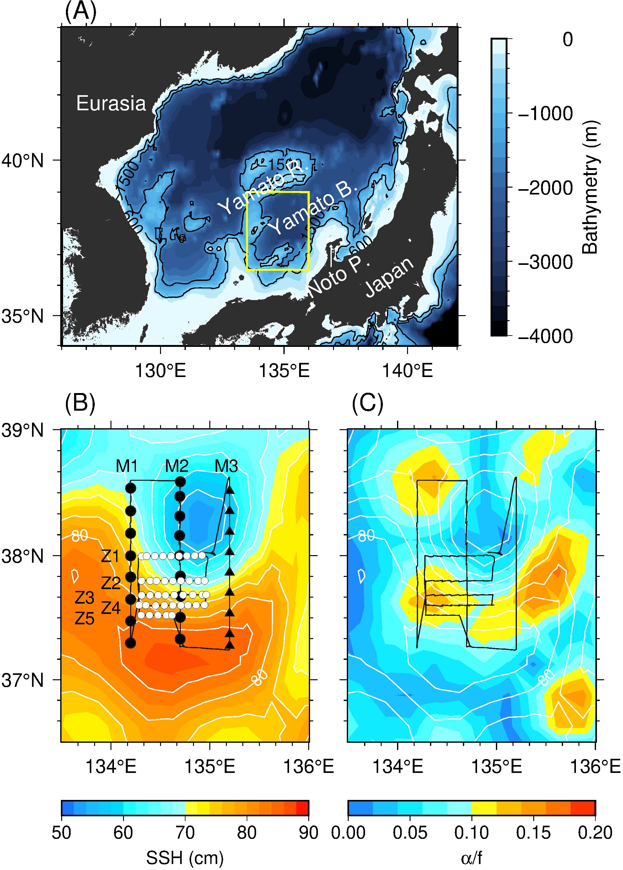
Figure 1. (A) Bathymetry around the study domain (yellow rectangle). Black lines indicate 600 and 1000 m isobaths. (B) locations of VMP (circles) and XCTD (triangles) stations and horizontal distribution of sea surface height (SSH; shading) on 27 June 2021. Closed and open circles denote the meridional (M1 and M2) and zonal (Z1–Z5) VMP sections, respectively. Black line indicates the ship’s track. (C) Horizontal distribution of strain rate (α; shading) normalized by f on 27 June 2021.White contours indicate the SSH at an interval of 4 cm.

Japan Fisheries Research and Education Agency (FRA) and Atmosphere and Ocean Research Institute (AORI) conducted a series of observation in the Japan Sea (called FATO: FRA-AORI TWC Observatory). Within the framework of the FATO project (Kawaguchi et al., 2020, 2021, 2023; Wagawa et al., 2020; Yabe et al., 2021), we carried out intensive observations of the multi-scale physical processes (i.e., meso-, submeso- and micro-scale features) at the periphery of the TWC front during June–July 2021. Over this study period, the spatial distribution of the sea surface height (SSH) revealed a southward-flowing meander of the TWC front (Figure 1B). We completed our the intensive survey across the western side of this meander crest. It is well known that convergent motion develops on the western side of such meander crests (Spall, 1995; Wang, 1993), and often coincides with the frontogenesis. In the present study, we monitored the submesoscale frontogenesis and submesoscale water mass patterns using in situ hydrographic data collected during the FATO observational campaign. We use these observations to evaluate the submesoscale frontogenesis quantitatively and consider how it affect turbulent-scale mixing.

The remainder of this paper is organized as follows. Section 2 describes the data acquisition during the campaign and the subsequent data processing. In section 3, we present the results of hydrographic surveys across the TWC front to show snapshots of the physical structures, and use high-density microstructure measurements to reveal the frontogenesis at the TWC front and the contribution of this frontogenesis, as well as resulting submesoscale water mass patterns, to the turbulent mixing. Section 4 considers the energy conversion caused by the frontogenesis and the analogy between the deformation of the TWC and that of the Kuroshio and mesoscale eddies as an example of other fronts, and presents the conclusions.

2 Materials and methods

2.1 Hydrographic data

The intensive survey was conducted using R/V Shinsei-maru of the Japan Agency for Marin–Earth Science and Technology (JAMSTEC) from 25 June to 2 July 2021, along three meridional (M1–M3) and five zonal (Z1–Z5) sections (Figure 1B). These sections were selected to resolve the detailed structure on the western side of the southward meander crest of the TWC front. The distance between the meridional lines was ~45 km, and that between Z1 and Z2 was ~20 km, and between the remaining zonal lines was ~9 km. Along all lines except M3, microstructure and hydrographic observations were conducted using a profiler (VMP-250; Rockland Scientific; hereinafter VMP) at horizontal intervals of approximately 20 and 10 km along the meridional and zonal sections, respectively. Temperature (T) and salinity (S) were measured using expendable conductivity–temperature–depth profilers (XCTD; Tsurumi Seiki, type 1) from the surface to a depth of 1000 m along M3.

Slow-response CTD sensors installed on the VMP acquired T and S at a sampling frequency of 64 Hz during descent. Raw data from the VMP-based CTD observations were compiled to produce 1-m averages down the vertical profiles after relevant post-screening procedures (Kawaguchi, 2019). Potential temperature (θ), potential density (σ_θ), and buoyancy were calculated using the T and S values obtained by the VMP-based CTD and XCTD. Buoyancy was calculated as follows:

$\begin{array}{ll}b=-g\rho /{\rho }_0,& (1)\end{array}$

where g is gravitational acceleration, ρ is the in situ density, and ρ₀ = 1028 kg m⁻³ is a reference density. The zonal (b_x) and meridional (b_y) derivatives of b (Equation 1) were calculated along each section to determine the strength of the TWC front and its temporal variability. x and y are zonal and meridional coordinates (positive eastward and northward), respectively, and subscripts denote the derivatives. In calculating the gradient, priority was given to obtaining the velocity shear over a wide area (making use of more data) rather than smoothing to adjust to the same level of horizontal resolution; i.e., along both the meridional and zonal lines, the x and y derivatives were determined from the forward difference. Along the meridional lines, the x and y derivatives were calculated at intervals of approximately 45 and 20 km, respectively, whereas both the x and y derivatives were calculated at intervals of approximately 9–10 km along zonal lines Z2–Z5. Because Z1 as away from the TWC front and Z2, the profiles along Z1 was not used in the gradient calculation. Note that the gradient characteristics remained unchanged when the resolution was adjusted to the zonal or meridional resolution. The value of spiciness (π) was defined through its differential:

$\begin{array}{ll}d\pi =\rho ({\alpha }_t d\theta +\beta dS),& (2)\end{array}$

where ${\alpha }_t=-{\rho }^{-1}(\partial \rho /\partial \theta )$ and $\beta =-{\rho }^{-1}(\partial \rho /\partial S)$ are the coefficients of thermal expansion and saline contraction, respectively. Note that, herein, the symbol π refers to spiciness, not the mathematical constant pi. The value of π is a useful density-compensated tracer for examining water transport along an isopycnal. The value of π (Equation 2) was calculated using the polynomial expansion of Flament (2002). The zonal (π_x) and meridional (π_y) derivatives of π were calculated using a similar equation to the calculation of the buoyancy gradient. In addition, the eastward geostrophic velocity (U) was calculated using the T and S profiles with a reference level of 1000 m along transect M3.

2.2 Microstructure data

The VMP collected high-resolution vertical profiles of current shear and temperature gradient at a temporal frequency of 512 Hz as it descended at around 0.5 m s⁻¹ from the surface to a depth of ~400 m. The dissipation rates of turbulent kinetic energy (ϵ) and the variance of the temperature gradient (χ) were evaluated by integrating the auto-spectral density along the vertical wavenumber coordinate. The integration limits for ϵ and χ were treated following Kawaguchi et al. (2021). The eddy diffusivity (K_z) was estimated using ϵ and the vertical buoyancy gradient (b_z)as follows (Osborn, 1980):

$\begin{array}{ll}{K}_z=0.2ϵ/b_z.& (3)\end{array}$

The thermal diffusivity based on χ (K_θ) was estimated as follows:

$\begin{array}{ll}{K}_{\theta }=\chi /2{\theta }_{z}2.& (4)\end{array}$

The diffusivity was evaluated using the dissipation rates and the diffusion coefficients (Equations 3, 4) in relation to the submesoscale frontogenesis and water mass patterns.

2.3 Deformation and ASC

Northward and eastward current velocities (u and v, respectively) were measured using a shipboard RDI 38-kHz acoustic Doppler current profiler (ADCP) at depth intervals of 16 m. These data were calibrated for angle misalignment using bottom tracking data (Joyce, 1989). The ship velocities were measured using the Global Positioning System. Current velocity profiles were estimated at intervals of 5 min. The current velocity profiles were further averaged between each VMP and XCTD station using ~15 profiles. This is to exclude the data immediately after leaving an observation point and before stopping because the speed of the vessel changes significantly at these points. We also calculated the zonal (u_x and v_x), meridional (u_y and v_y), and vertical (u_z and v_z) derivatives of u and v, where z indicates the vertical coordinates (positive upward), in a similar manner to calculating the buoyancy gradient for the horizontal difference.

We used the absolute SSH data set produced and distributed by the Copernicus Marine and Environment Monitoring Service (https://marine.copernicus.eu/) provided on a 0.25° × 0.25° grid to detect the deformation flow near the TWC front. We calculated the lateral strain rate (α) to measure the deformation, which can cause frontogenesis. The rate was derived as follows:

$\begin{array}{ll}\text{ α}= {[{({U^g}_x-{V^g}_y)}^2+{({V^g}_x+{U^g}_y)}^2]}^{1/2}={({\sigma }_n+{\sigma }_s)}^{1/2},& (5)\end{array}$

where U^g = −(g/f₀)h_y and V ^g = (g/f₀)h_x are the zonal and meridional geostrophic velocities calculated from SSH (h), respectively, and σ_n and σ_s are the normal and shear components of strain, respectively. The large value of α contributes to frontogenesis when it induces convergence in the cross-frontal direction and elongation along the frontal axis. Conversely, attention must be paid to the fact that divergence in the cross-frontal direction may result in frontolysis. When the value of α is as large as O(10⁻⁵ s⁻¹), the deformation is likely to be driven by the background mesoscale confluence (Nagai et al., 2009). The value of α was estimated to be ~1.0 × 10⁻⁵ s⁻¹ (not shown) and that normalized by f was >0.1 on the western side of the southward meander crest of the TWC front (Figure 1C). The estimated range of α for the downstream region of TWC was slightly smaller than that reported for the Kuroshio deformation area (Ito et al., 2023; Nagai et al., 2009). As the intensity of the TWC is modest compared with the Kuroshio, the TWC frontogenesis is more likely to develop from the perspective of the value of α in the observed area. In addition, the estimate of α in the ocean interior was obtained by replacing U^g and V^g in Equation 5 with the ADCP-measured u and v to examine the deformation in the ocean interior.

To evaluate the evolution of the deformation and frontogenesis, we calculated the temporal evolution of the horizontal buoyancy gradient as follows (Hoskins, 1982):

$\begin{array}{ll}\frac{D}{Dt}{\mathrm{\nabla }}_{h}b = \left[\begin{array}{c}-u_x{b}_x-v_x{b}_y\\ -u_y{b}_x-v_y{b}_y\end{array}\right]\equiv \left[\begin{array}{c}{Q}_1\\ Q_2\end{array}\right]=\mathbf{Q},& (6)\end{array}$

where b is assumed to be forced by a horizontal two-dimensional, nondivergent flow. According to Equation 6, the components of the Q-vector (i.e., Q₁ and Q₂) may cause the temporal variation in the frontal structure in the zonal and the meridional directions, respectively. The first and second terms in Q₁ (Q₂) represent the stretching (tilting) and tilting (stretching) components, respectively. An intensification of the horizontal density gradient, indicative of increased b gradient, enhances the contrast between light and dense water masses, i.e., frontogenesis. Nevertheless, when shear flow causes a reorientation of the gradient from one axis to another, the resulting increase of gradient cannot be simply interpreted as frontogenesis. The temporal evolution of π was examined by replacing b_x and b_y in Equation 6 with π_x and π_y:

$\begin{array}{ll}\frac{D}{Dt}{\mathrm{\nabla }}_h\pi = \left[\begin{array}{c}-u_x{\pi }_x-v_x{\pi }_y\\ -u_y{\pi }_x-v_y{\pi }_y\end{array}\right]\equiv \left[\begin{array}{c}{Q_1}^{\pi }\\ {Q_2}^{\pi }\end{array}\right]=\mathbf{\text{Q}}.& \text{(6')}\end{array}$

An increase in the π gradient indicates the convergence of water masses with different properties, regardless of whether their density difference. Therefore, this parameter serves as an indicator for evaluating the convergence and fragmentation of water masses with distinct properties associated with frontogenesis.

Assuming that the strengthening of the front by the deformation is slumped and balanced by the frictionally driven ASC (Nagai et al., 2008; Thomas and Ferrari, 2008; Thompson, 2000) under steady-state, the Boussinesq approximation, and a constant eddy viscosity coefficient, the two-dimensional scaling relationship in zonal fronts, based on the governing equation for a density current with removal of the advective terms, is as follows (Garrett and Loder, 1981; Nagai et al., 2009):

$\begin{array}{ll}{K}_v{u}_{zzy}=f{v}_y,& (7)\end{array}$

where K_v is the vertical eddy viscosity coefficient. Note that v_y is the stretching component of α in the along-front direction; i.e., the frontogenesis caused by the stretching fluid motion is offset by the eddy viscosity. In addition, when only the frontogenesis is initiated by the deforming motion of the fluid, the ASC may traverse the zonal front and then produce a diapycnal buoyancy flux ($F_b$) that can be estimated as follows (McWilliams, 2016):

$\begin{array}{ll}{F}_b~w^{\prime }{b}^{\prime }~\alpha h^2{b}_{x}2/f^2,& (8)\end{array}$

where h is the turbulent boundary layer thickness. The total buoyancy flux is obtained by integrating Equation 8 throughout the cross-section.

Furthermore, the magnitude of the vertical velocity driven by the ASC (w_ASC) associated with the zonal oriented front was estimated more quantitatively by inverting a simplified 2D version of the omega equation (i.e., the quasi-geostrophic form of the Sawyer–Eliassen equation [Hoskins et al., 1978]) as follows:

$\begin{array}{ll}{(N^2{w}_{\text{ASC}})}_{yy}+f^2{w}_{\text{ASC}}\mathrm{zz}=2g{(v_y{\rho }_y)}_y/{\rho }_0,& (9)\end{array}$

where N² = −(g/ρ₀)∂ρ/∂z is the buoyancy frequency. We calculated the buoyancy anomaly ($b\text{'}$) as the difference between in situ buoyancy and the along-front mean buoyancy. Then, the conversion from the available potential energy to the kinetic energy (i.e., adiabatic vertical buoyancy flux; C_ASC) was calculated as follows:

$\begin{array}{ll}{C}_{\text{ASC}}=w_{\text{ASC}}{b}^{\prime }.& (10)\end{array}$

The integrated value of the C_ASC along the section provides a quantitative estimate of energy contribution from the ASC to the flow including turbulence.

3 Results

3.1 General features of the TWC front

During the study period (June–July 2021), the TWC was meridionally confluent around the western side of the southward meander crest (around 37.6°N on the M1 and M2 transects; Figure 2) and divergent in the downstream region (around 37.4°N on the M3 transect). Cyclonic and anticyclonic eddies were located to the north and south, respectively, of the TWC (herein referred to as CE and ACE, respectively). The southward flow (0.2–0.5 m s⁻¹) along the TWC meander was captured north of the M1 and M2 transects, in the track between M1 and M2, and along Z1 and Z2. The southward flow changed its main-axis orientation from the southeast to eastward as the location of the survey moved south (around 37.6°N). A northward to northeastward flow with a speed of 0.1–0.3 m s⁻¹ was observed near the southern end of the M1 and M2 transects and along the track between M2 and M3. Therefore, in the upstream section of the observation area (i.e., on the western side of the southward meander crest), there was convergent flow in the cross-front direction. The velocity of the converging flow exceeded 0.7 m s⁻¹ south of the M2 transect and east of Z4 and Z5. South of M3 across the downstream area of the TWC front, the TWC flowed in a northeastward direction to the north of the front, but in a southeastward direction to the south of the front. This convergence and divergence are consistent with theoretical studies (Spall, 1995; Wang, 1993) and in situ observations in the Kuroshio region (Ito et al., 2023).

Figure 2

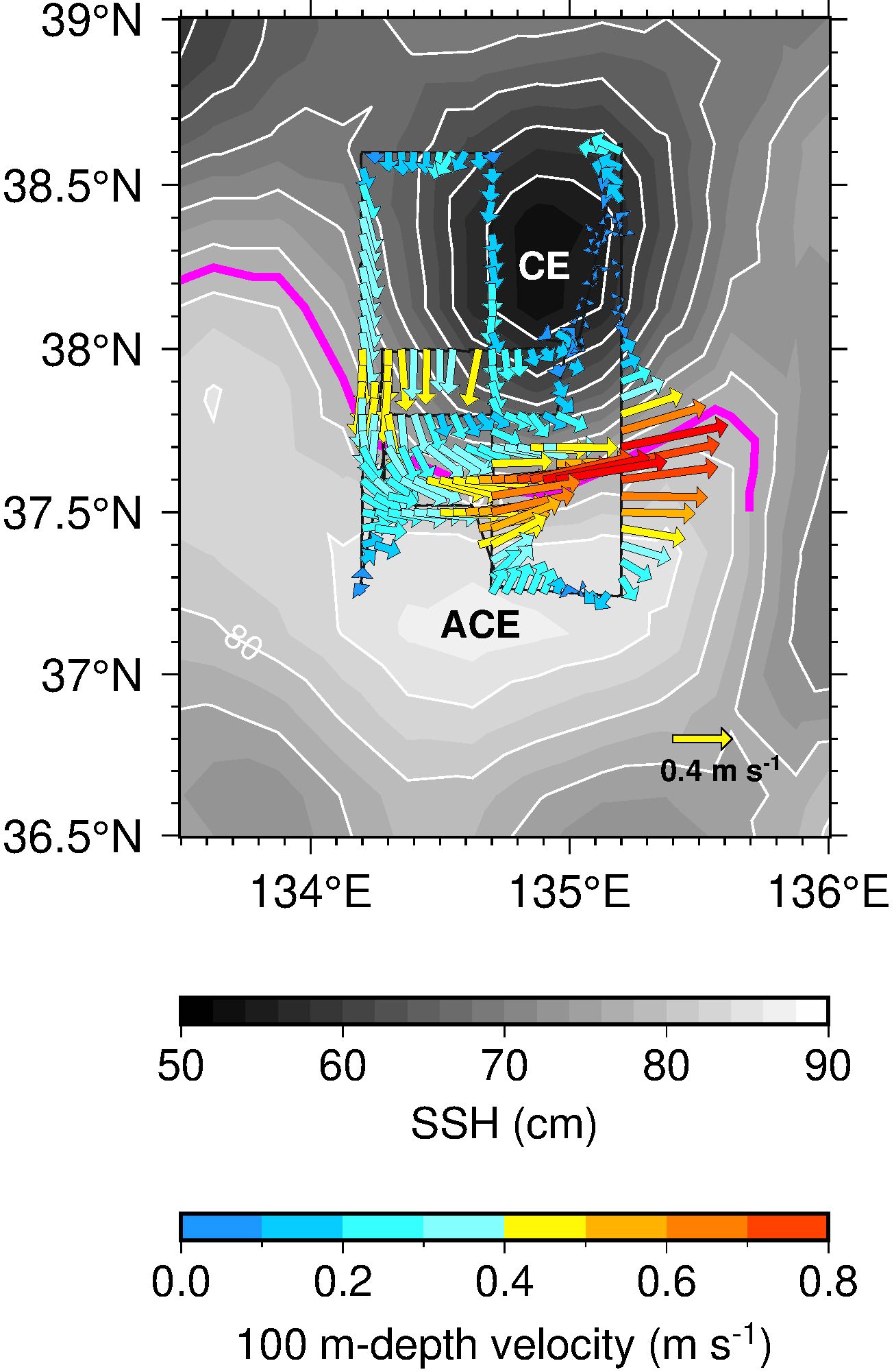
Figure 2. Horizontal velocity (m s⁻¹) at a depth of 100 m observed by ADCP (arrows). Black line is the ship’s track, and white contours indicate the SSH at an interval of 4 cm. Magenta line indicates the main-axis of the TWC. CE (ACE) denotes the center of the cyclonic (anticyclonic) eddy north (south) of the TWC.

The survey along the M3 transect, which was undertaken to capture the general water mass structure, showed well-defined TWC frontal structures (Figure 3). A density level of 26.4σ_θ resided around 300 m depth near the latitude of 37.42°N, whereas it shoaled up to 50 m around 38.26°N. This is plausibly accounted for by isopycnal heaving resulting from the CE (Figure 2). The CE served to uplift the Japan Sea Proper Water, characterized by θ ≈ 1°C and S ≈ 34.1, to a depth of about 150 m (Figures 3A, B). South of the isopycnal slope, a distinct water mass characterized by warm (θ > 14°C) and saline (S > 34.3) properties was found, particularly between the surface and a depth of 50 m. In contrast, a thick subsurface water mass with θ ≈ 11°C and S ≈ 34.1 was present between depths of 100 and 250 m. A large negative horizontal density gradient (i.e., the TWC front) was observed between the warm water mass within the ACE and the CE (Figure 3G). According to our calculation of the geostrophic balance, the zonal geostrophic velocity (U) was 0.6 m s⁻¹ (Figure 3D), and the zonal velocity measured by the ADCP (u) was approximately 0.7 m s⁻¹ (Figure 3E) in the TWC front. As confirmed from the plan view of the horizontal velocity (Figure 2), there was also a northward (southward) component north (south) of the front around 37.6° N (Figure 3F).

Figure 3

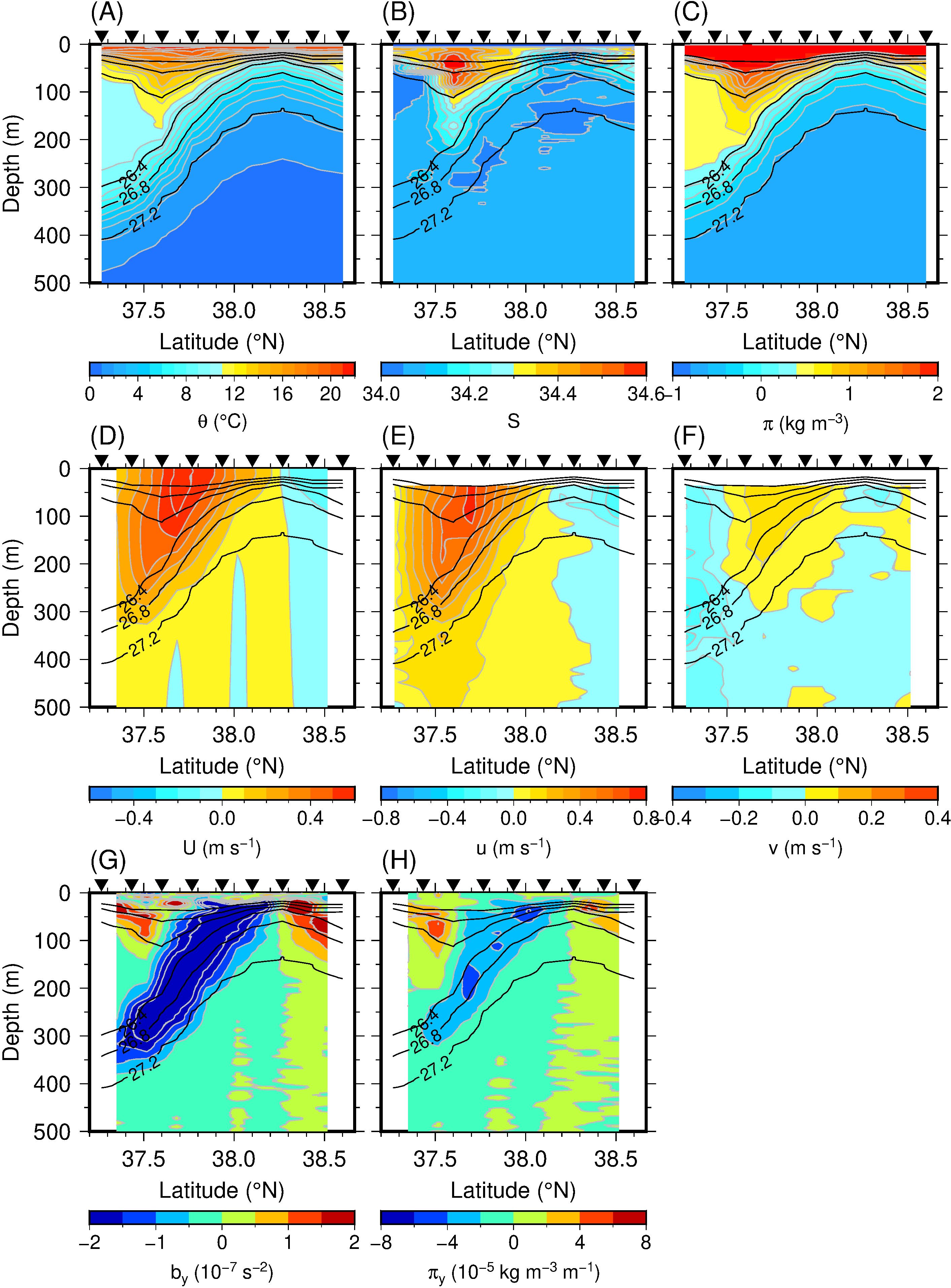
Figure 3. Sections of (A) θ (°C), (B) S, (C) π (kg m⁻³), (D) U (m s⁻¹), (E) u (m s⁻¹), (F) v (m s⁻¹), (G) b_y (10⁻⁷ s⁻²), and (H) π_y (kg m⁻³ m⁻¹) along the M3 transect. Black inverted triangles at top of each panel indicate XCTD stations. Black lines denote σ_θ with a contour interval of 0.4 kg m⁻³ from 25.2 to 27.2 kg m⁻³.

Patches of warm and saline (i.e., high π) water with a horizontal scale of <20 km were observed near the TWC front (Figures 3A–C). In the surface layer, a patch with S > 34.6 was centered at a depth of 50 m around 37.60°N, which was a thick structure compared with the ambient water. In its lower layer, a patch with a local maximum of θ ≈ 11–13°C and S ≈ 34.3 was found at a depth of 170 m. A similar patch was also observed along the M1 and M2 transects (Figure 4), suggesting that they constituted a submesoscale filament. Inside this patch, π was greater (≈ 0.7 kg m⁻³) than in the surrounding water at the same depth (Figure 3C). The slight difference in π was evident when calculating its gradient (Figure 3H). The near-surface and deeper patches of high π values described above present as large values of π_y (≈ 4 × 10⁻⁵ kg m⁻³ m⁻¹ around 37.5°N centered at a depth of 75 m, and ≈ −4 × 10⁻⁵ kg m⁻³ m⁻¹ around 37.7°N centered at a depth of 200 m, respectively). Slightly less saline (S < 34.05) water than the surroundings was observed in the upper part of the thick uniform layer south of the TWC front and along the 27.2σθ isopycnal in the front and inside the CE (Figure 3B). However, this salinity patch was compensated by the temperature and did not present as extrema values of π and π_y (Figures 3C, H).

Figure 4

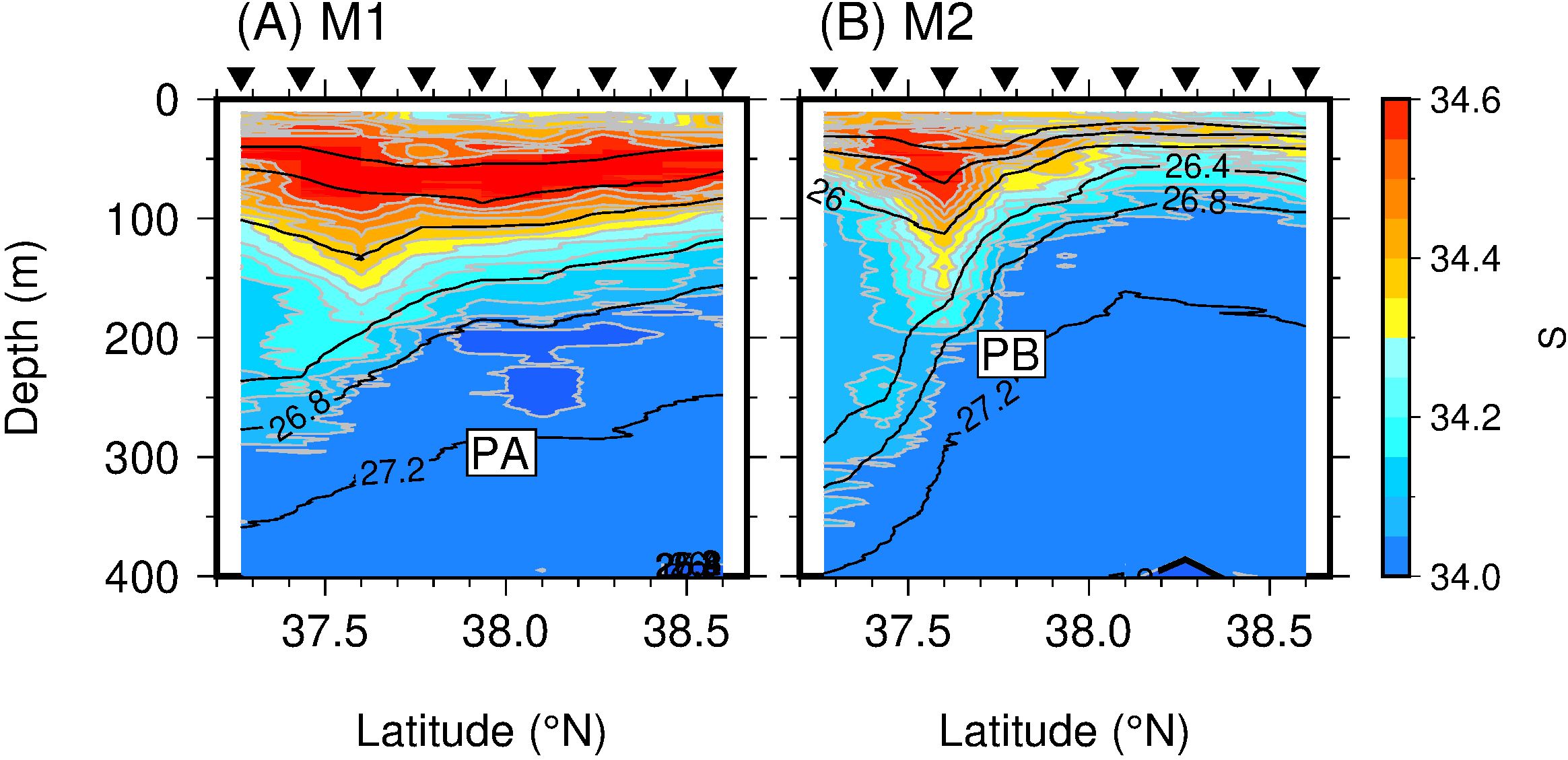
Figure 4. Sections of S along the (A) M1 and (B) M2 transects. Black inverted triangles at top of each panel indicate VMP stations. Black lines denote the observed VMP σ_θ with a contour interval of 0.4 kg m⁻³ from 25.2 to 27.2 kg m⁻³. PA and PB denote the low- and high-S patches, respectively.

We examined the S distribution to confirm the water mass pattern along the M1 and M2 transects (Figure 4). It should be noted that the distribution of S along M3 is already illustrated in Figure 3B. The general structure was similar to that along M3 (Figure 3B). Focusing on the patchy structure, we found a patch with S > 34.6 centered at a depth of 50 m around 37.60°N along M1 and M2, with convex downward isopycnals (Figure 4). Below this patch, another patch with S ≈ 34.1–34.4 was found, and was particularly well developed along M2 (Figure 4B). A similar structure was also recognized along M3, suggesting that they constituted a submesoscale filament. A low-S (S < 34.0) patch was centered at 38.1°N at depths of 200–250 m along M1 (Figure 4A). A similar low-S patch was also observed along M3, albeit at a slightly different location and with slightly different S values (Figure 4B). The low-S patch along M1 and the vertically aligned high-S patch along M2 are herein referred to as PA (patch A) and PB (patch B), respectively.

3.2 Deformation flow and frontogenesis

The Velocity shear between the M1 and M2 transects showed deformational flow causing frontogenesis near the TWC front (Figure 5). The value of u_x was positive near the front, indicating an increase in the eastward velocity downstream (from M1 to M2; Figure 5A). The value of v_x was large at the northern end of the front in the surface layer, with the northward component increasing downstream (Figure 5B). Large values were also centered around 38°N at a depth of 400 m. The southwestern end of the Yamato Ridge (water depth of 500–600 m) is located in this region (Figure 1A), and the velocity shear caused by the influence of the bottom topography appears to have been captured. As anticipated, the value of u_y was positive south of the velocity maximum and negative north of it (Figure 5C). This is because, to the south (north) of the velocity maximum, the eastward velocity increases (decreases) toward the north. A large negative v_y value was recorded near the front, indicating convergent flow in the cross-front direction (Figure 5D). The value of σ_n near the front was positive (Figure 5E; σ_n > 3 × 10⁻¹⁰ s⁻²) due to the positive u_x and negative v_y (Figures 5A, D) there. Large negative and positive values of v_y over the Yamato Ridge could cause convergence and divergence, respectively, in the cross-front direction. Between the M1 and M2 transects, the contribution of σ_s was not as large as that of σ_n (Figure 5F). Thus, the contribution of σ_n relative to α was significant, and the strong deformation flows (α/f > 0.2) caused the TWC frontogenesis. This value of α is larger than that estimated from the SSH (Figure 1C) and comparable to that reported in previous studies (Nagai et al., 2009; Ito et al., 2023) for the occurrence of frontogenesis in the Kuroshio region. In addition, the condition α/f < 1 indicates that the frontal sharpening stage was exponential rather than super-exponential (Hoskins and Bretherton, 1972), supporting the interpretation that frontogenesis was driven by the deformation flow rather than the convergence of the ASC. The strong deformation associated with the TWC front is herein referred to as DA (deformation A), and that over the Yamato Ridge as DB (deformation B; Figure 5G).

Figure 5

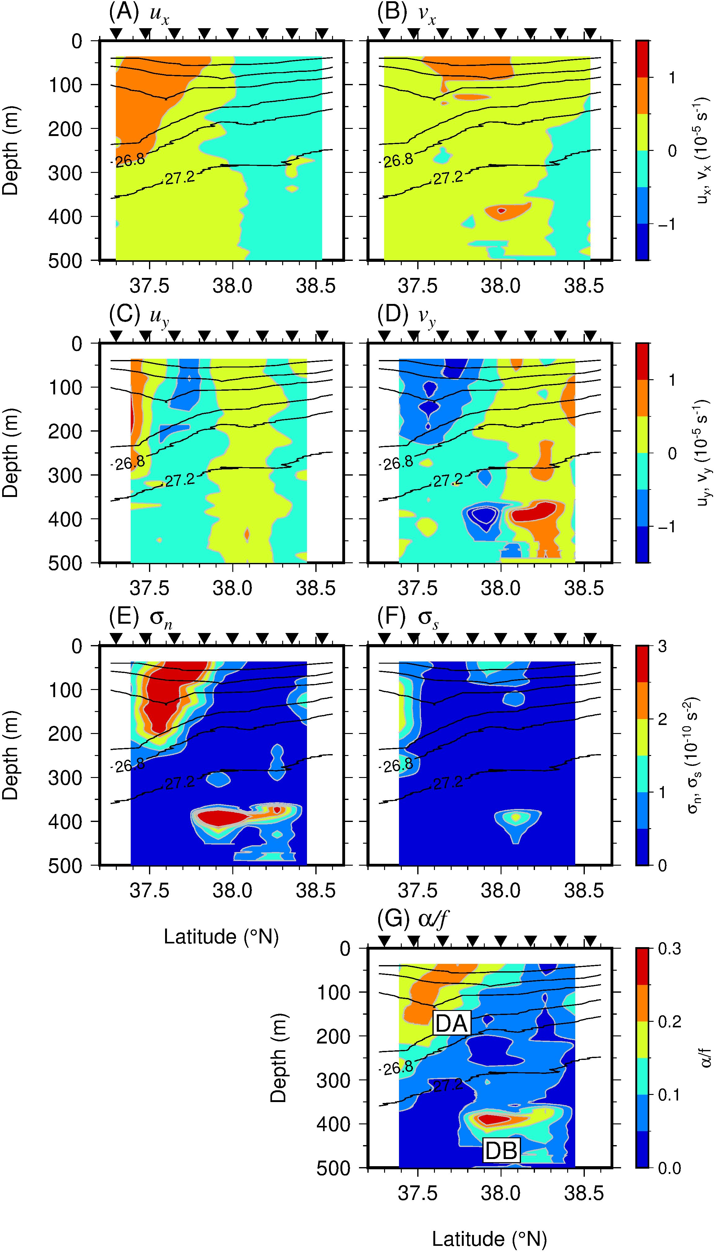
Figure 5. Sections of (A) u_x (10⁻⁵ s⁻¹), (B) v_x (10⁻⁵ s⁻¹), (C) u_y (10⁻⁵ s⁻¹), (D) v_y (10⁻⁵ s⁻¹), (E) σ_n (10⁻¹⁰ s⁻²), (F) σ_s (10⁻¹⁰ s⁻²), and (G) α normalized by f between the M1 and M2 transects. Black inverted triangles at top of each panel indicate VMP stations. Black lines denote observed VMP σ_θ with a contour interval of 0.4 kg m⁻³ from 25.2 to 27.2 kg m⁻³. DA and DB in (G) denote the strong deformation associated with the TWC front and the Yamato Ridge, respectively.

Deformation flow was also present between the M2 and M3 transects, while the stretching in the along-front direction and convergence in the cross-front direction weakened, and the contribution of the velocity shear increased (Figure 6). The values of u_x and v_y near the TWC front were positive and negative, respectively (Figures 5A, D), but their magnitudes were not as large as those upstream (Figures 5A, D). Thus, the value of σ_n was also relatively small (Figure 6E). Negative (positive) values of v_x south (north) of the front were consistent with divergence downstream (Figure 6B). The value of u_y was particularly large between M2 and M3 (Figure 6C). This shear can increase the meridional gradient by tilting the tracer gradient in the zonal direction (Equation 6). As a result, the value of σ_s was large in the subsurface layer of the TWC front (Figure 6F; at depths of 100–300 m around 37.6°N), which was also reflected in the value of α (Figure 6G; herein, DC: deformation C).

Figure 6

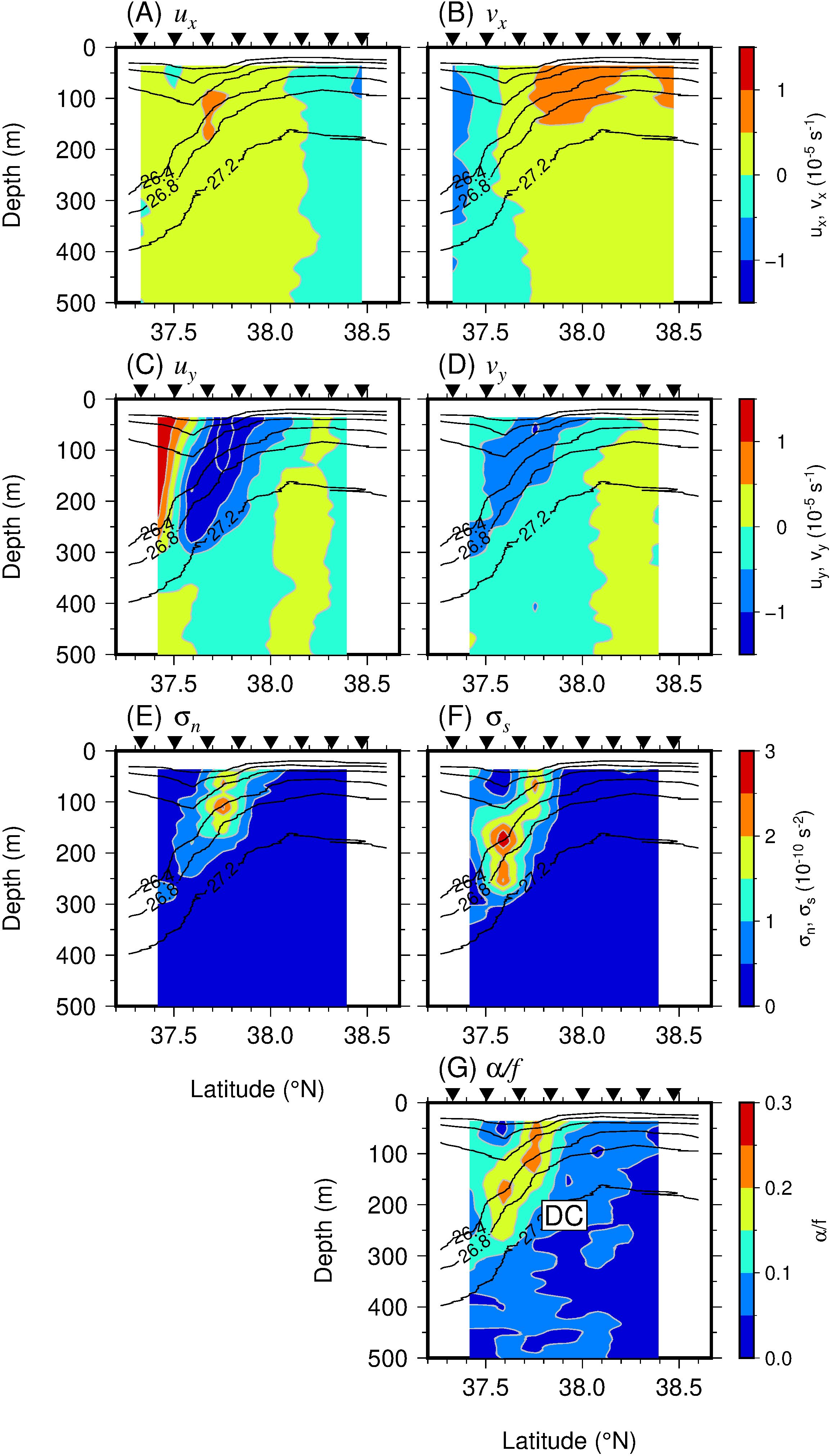
Figure 6. As for Figure 5, but between the M2 and M3 transects. DC in (G) denotes the strong deformation associated with the TWC front.

The velocity distribution identified in the meridional transects is expanded in the higher-resolution zonal transects shown in Figure 7. Here, we show the velocity shear between Z3 and Z4 (Figure 1B), where the feature was pronounced because the transects were close to the TWC front (Figure 1B). The zonal stretching (Figure 7A) and the meridional convergence (Figure 7D) in the surface layer (from the surface to a depth of 150 m) were consistent with the velocity distribution identified in the meridional transects (Figures 5, 6). As the TWC changed its main-axis direction from southward to eastward, the southward component of v became small east of the section (Figure 2). Thus, the sign of v_x was positive (Figure 7B). Due to this turning of the TWC, the eastward velocity was large toward the south in the surface layer; i.e., the value of u_y was negative (Figure 7C). At depths below 250 m, there were partial areas with a pronounced eastward velocity turning north (i.e. u_y > 0), and this trend was particularly clear along the intermediate line between Z3 and Z4.

Figure 7

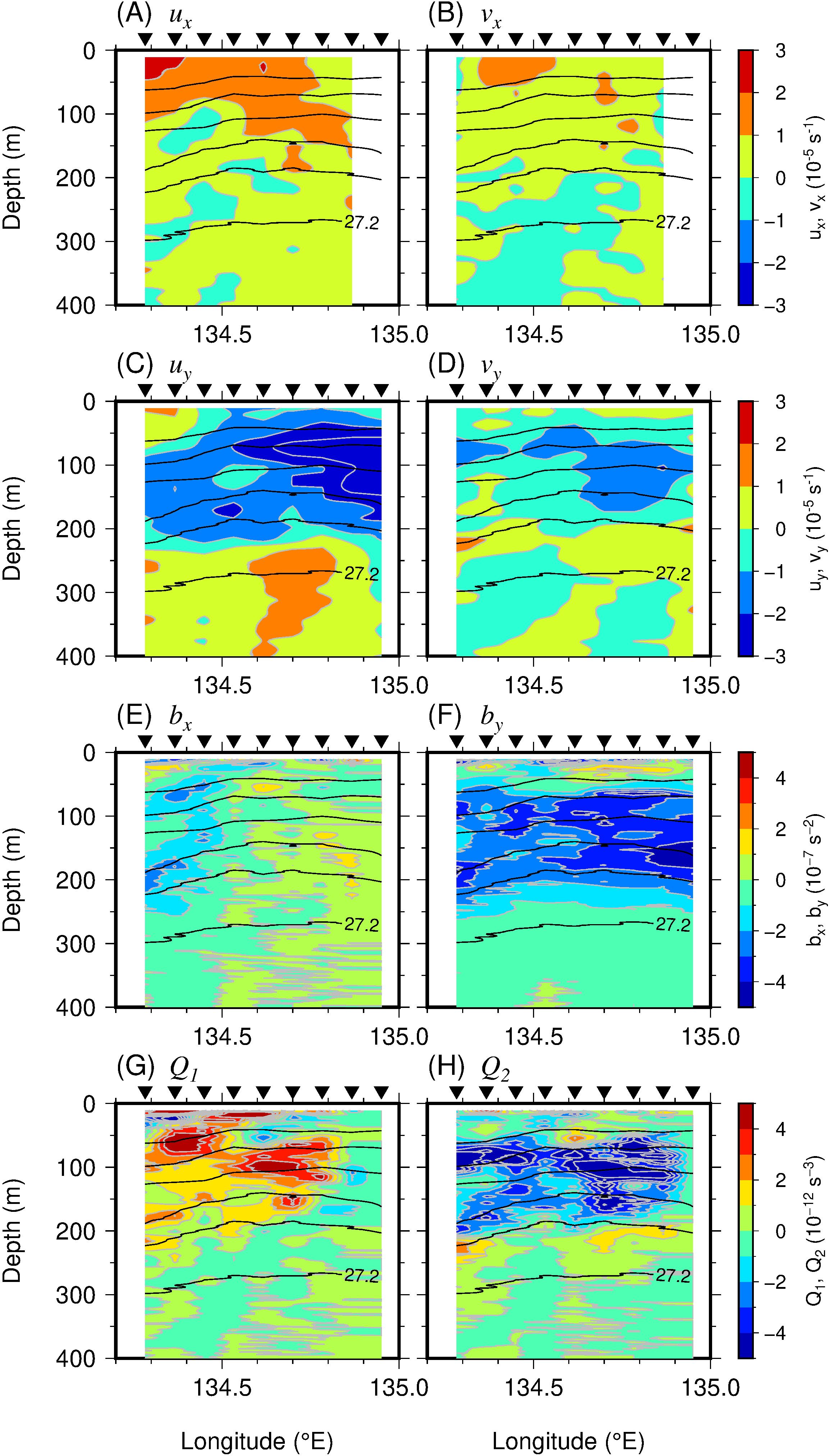
Figure 7. Sections of (A) u_x (10⁻⁵ s⁻¹), (B) v_x (10⁻⁵ s⁻¹), (C) u_y (10⁻⁵ s⁻¹), (D) v_y (10⁻⁵ s⁻¹), (E) b_x (10⁻⁷ s⁻²), (F) b_y (10⁻⁷ s⁻²), (G) Q₁ (10⁻¹² s⁻³), and (H) Q₂ (10⁻¹² s⁻³) between the Z3 and Z4 transects. Black inverted triangles at top of each panel indicate VMP stations. Black lines denote observed VMP σ_θ with a contour interval of 0.4 kg m⁻³ from 25.2 to 27.2 kg m⁻³.

The temporal evolution of the buoyancy gradient (Equation 6) calculated using the zonal transects showed a marked increase in terms of the meridional component gradient (i.e., frontogenesis) on the western side of the southward meander crest of the TWC (Figure 7). The absolute value of the buoyancy gradient in the meridional direction was broadly more pronounced than that in the zonal direction (Figures 7E, F). The sign of b_x turned from negative to positive around 134.6°E (Figure 7E). This is because, on the western side of the section, the TWC flowed slightly southeastward (Figure 1B), resulting in a warm water mass to the west and cold water to the east, while on the eastern side of the section the TWC turned slightly northeastward, resulting in cold water to the west and warm water to the east. The sign of b_y was negative at depths of 50–200 m (Figure 7F). This negative value was particularly significant east of the section where the TWC front was oriented almost zonally. These buoyancy gradients were forced by the horizontal velocity shear, resulting in the weakening of b_x (Figure 7G) and the strengthening of b_y (Figure 7H). Specifically, relative to the positive Q₁, the contribution of the tilting of the negative b_y due to the positive v_x was large (not shown, but can be deduced from Figure 7) because the contribution of b_y exceeded that of b_x. At the same time, the convergence of b_y caused by the negative v_y was significant in terms of creating the negative Q₂. On the other hand, the tilting of the b_x also contributed to forming the negative Q₂ because the value of u_y was moderately efficient. In particular, on the western side of the section around 134.3–134.4°E at depths of 50–250 m, the isopycnal surface characterized by a negative b_x (Figure 7E) was tilted by the negative u_y (Figure 7C), resulting in a negative b_y (Figure 7H).

The temporal variation of the spiciness gradient (Equation 6') also showed similar characteristics to those of the buoyancy gradient (Figure 8). Both the zonal and meridional gradients of spiciness were consistent with the water mass distribution in which warm and cold water masses were located to the south and north, respectively, of the transect (Figures 8A, B). The gradient was forced by the velocity shear (Figures 7A–D); therefore, the positive x-component of the Q-vector for π (Q₁^π) and the negative y-component of the same (Q₂^π) were found in the surface layer (Figures 8C, D). The deformation flow can also cause fragmentation of the density-compensated tracer due to the stretching and tilting of the water mass. Such fine structures would be captured as patches of θ, S, and π in the observed section (Figures 3A–C; as confirmed in section 3.1).

Figure 8

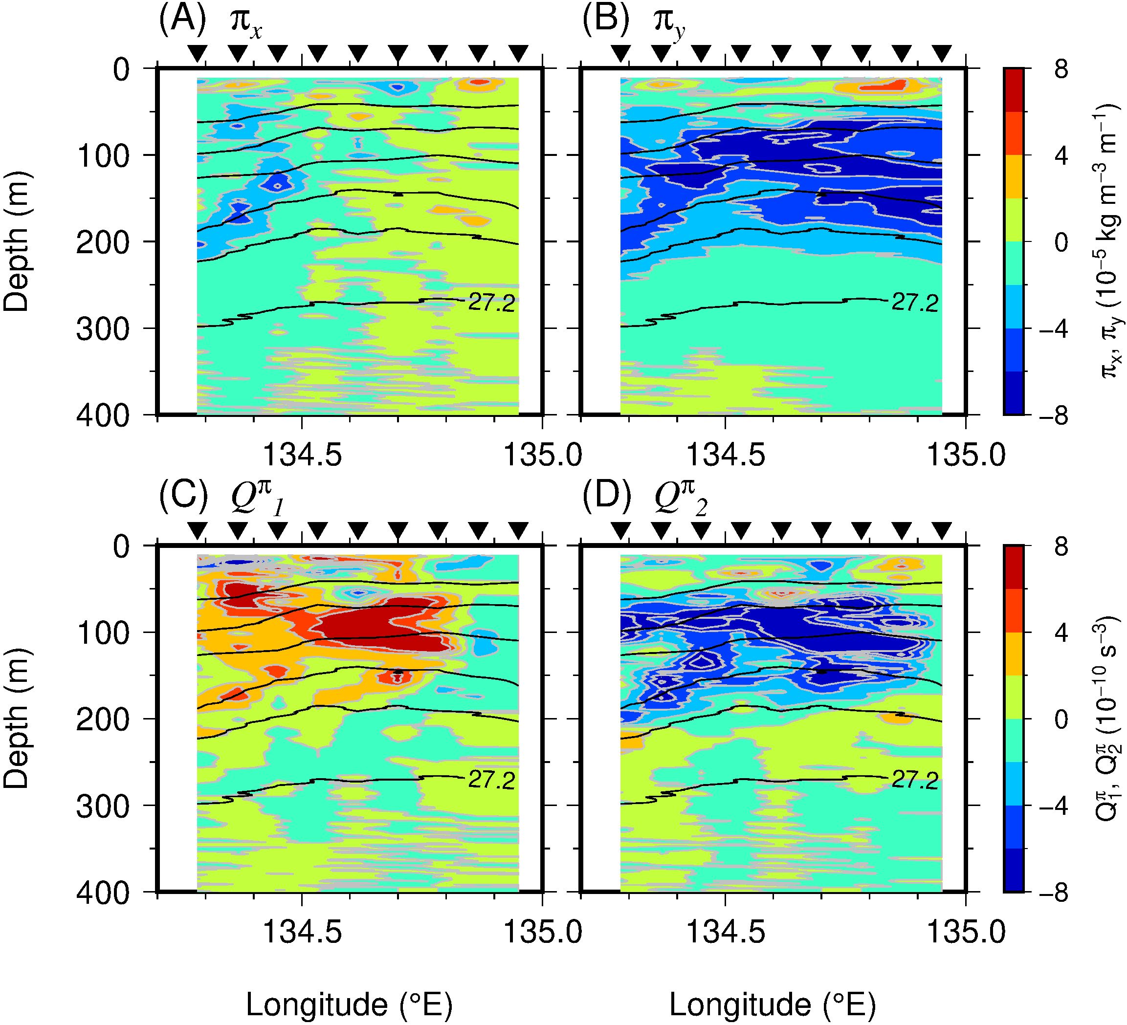
Figure 8. As for Figures 7E–H, but for the temporal evolution of π.

3.3 Impact on the turbulence

The observed value of ϵ increased near the large deformation flow (Figures 9A, B). In the subsurface layers shallower than 100 m, the magnitude of ϵ exceeded O(10⁻⁹ W kg⁻¹). In particular, in the subsurface layer, large values of ϵ were observed in and near the large-α area; i.e., at a depth of 50 m around 37.4°N (inside DA) on M1 (Figure 9A), and at depths of 50 m around 37.9°N (at the periphery of DC), 150–200 m around 37.75°N (also at the periphery of DC), and 300 m around 37.3–37.4°N (right beneath DC) along the M2 transect (Figure 9B). In addition, the value of ϵ was large over the southwestern end of the Yamato Ridge (at a depth of 400 m around 38.0°N, inside DB) Along M2, areas of large deformation flow corresponded to the edge of PB at depths of 150–200 m around 37.75°N (Figure 9D).

Figure 9

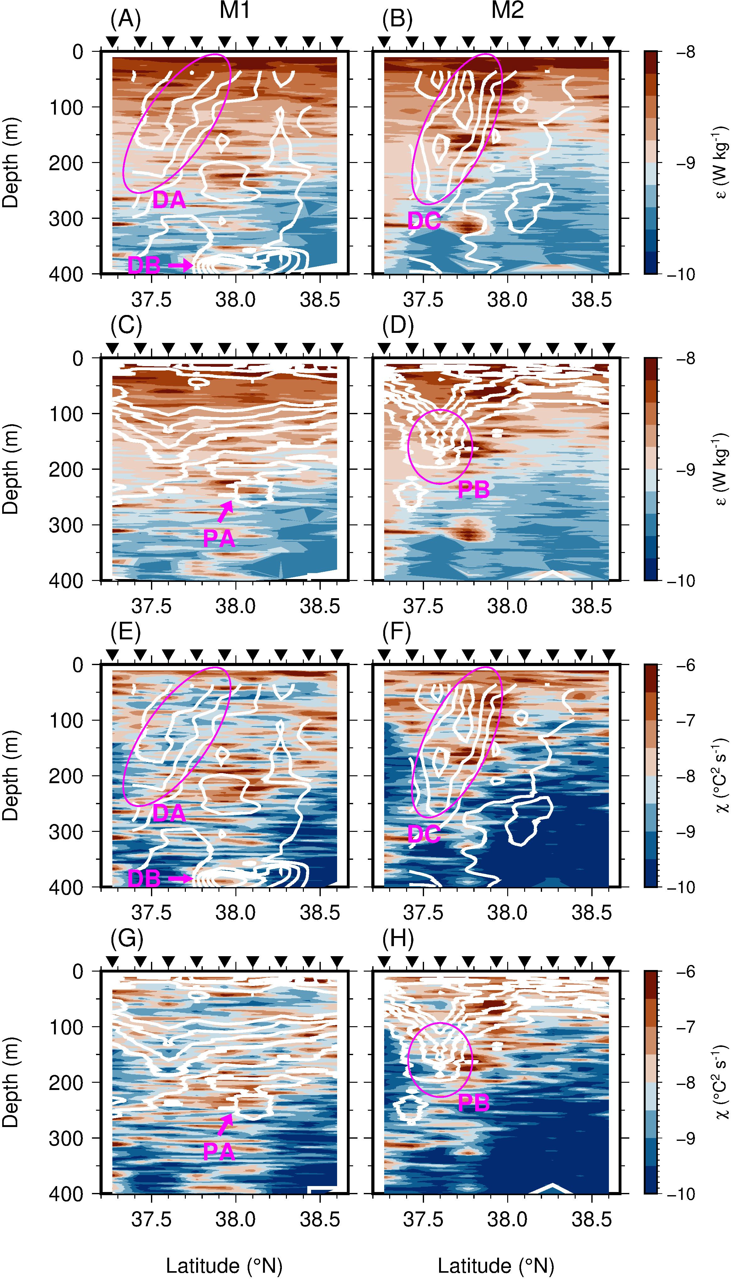
Figure 9. Sections of (A–D) ϵ (W kg⁻¹) and (E–H) χ (°C² s⁻¹) on a logarithmic scale along the M1 (left column) and M2 (right column) transects. Black inverted triangles at top of each panel indicate VMP stations. White lines in (A, B, E, F) denote α/f with a contour interval of 0.05 from 0 to 0.3 (see also Figures 5G, 6G). White lines in (C, D, G, H) denote S with a contour interval of 0.1 from 34.0 to 34.6 (see also Figure 4). DA, DB, DC, PA, and PB denote the strong deformations and the salinity patches. The shading is the same in each of (A, C), (B, D), (E, G), and (F, H).

The distribution of χ corresponded to that of the S patches and the large deformation flow (Figures 9E–H). Typically, the value of χ was large in regions where the value of ϵ was large, but only the value of χ was large [O(10⁻⁶°C² s⁻¹)] near the low-S patch (PA) centered at a depth of 200 m around 38.1°N (Figure 9G). This distribution suggests that even in areas where there is no dynamic deformation, the pattern of the water mass that appeared as traces of deformation can still develop turbulent mixing.

The vertical diffusivity was also large near the large-α area and the low-S patches (Figure 10). The value of K_z was large [O(10⁻⁴ m² s⁻¹)] over a wide area inside the warm water mass in the ACE south of the TWC front and also inside the cold water mass in the CE at depths below 200 m north of the front due to weak stratification (Figures 10A, B). A particularly large value of K_z [O(10⁻³ m² s⁻¹)] was observed in association with the DB signature (Figure 10A). In addition, along the M2 transect, K_z reached O(10⁻³ m² s⁻¹) inside and near the edge of DC, especially at depths of 50 m around 37.95°N and 300 m around 37.75°N (Figure 10B). The distinct signatures of the elevated K_z and the salinity patches (PA and PB) were not closely correlated (Figures 10C, D). The spatial distribution of K_θ was generally similar to that of K_z, but the value of K_θ was still large in terms of the spatial association with PA centered at a depth of 200 m around 38.1°N (Figure 10G). Strong turbulent mixing was expected near the strong deformation, rather than in areas of strong deformation, although the density gradient associated with the front was large. In addition, water mass patterns such as patches, filaments, and water mass fragmentation at the periphery of the front can induce efficient mixing.

Figure 10

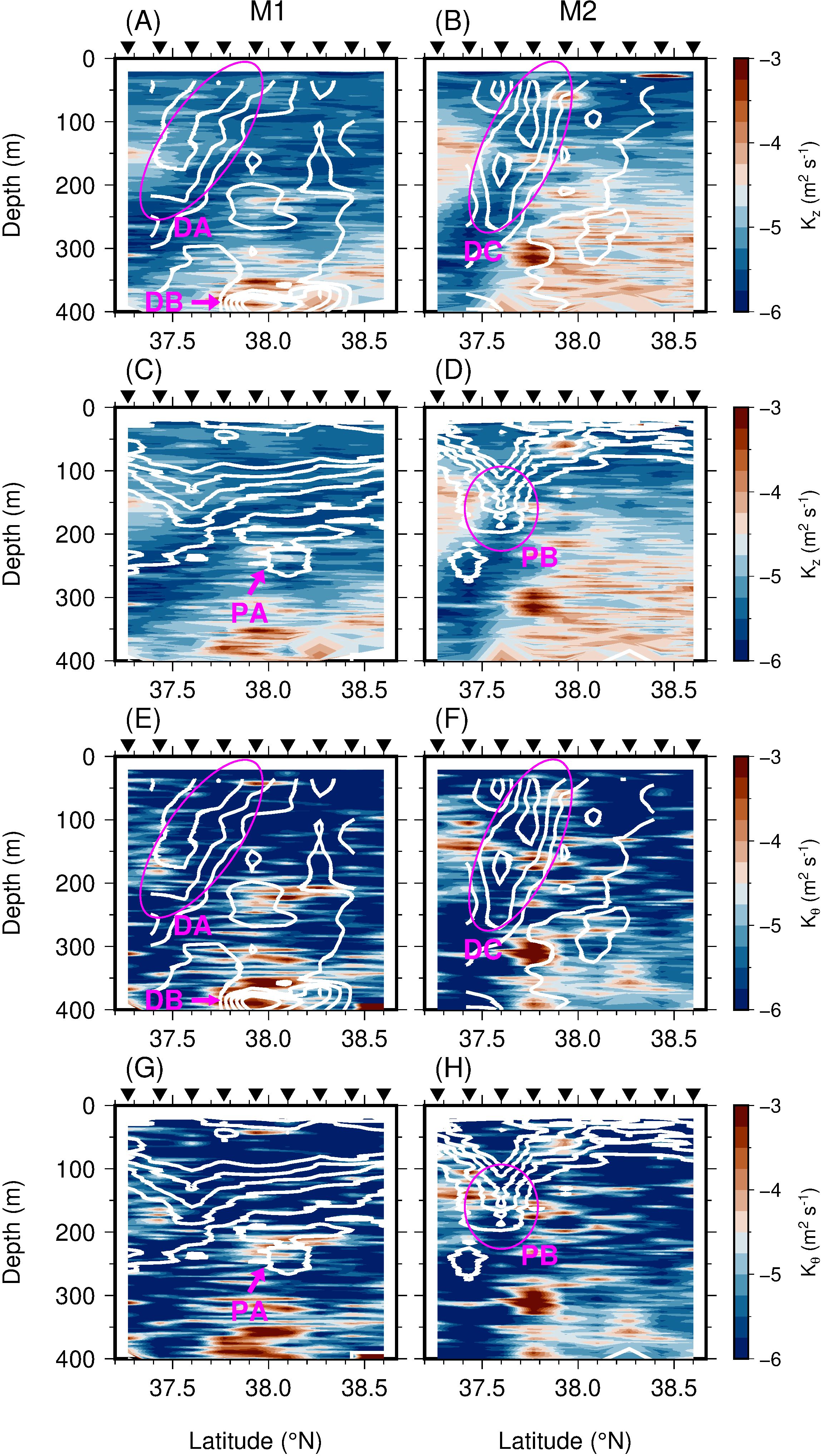
Figure 10. As for Figure 9, but for (A–D) K_z (m² s⁻¹) and (E–H) K_θ (m² s⁻¹) on a logarithmic scale.

There was no significant difference between the vertical shear of the geostrophic flow (U_z) and that of the zonal velocity obtained by the ADCP (u_z) along the M3 transect, where the geostrophic velocities were calculated (Figures 11A–C). The magnitudes of U_z (Figure 11A) and u_z (Figure 11B) coincidentally increased over the TWC frontal structure, where there was little difference between these two values (Figures 11C). Relatively large differences were evident near the center of the CE at a depth of 100 m around 38.0–38.5°N. There were also differences near the pycnocline that has a convex downward shape below the ACE south of the front, where negative values of u_z were observed (at a depth of 350 m around 37.4°N and at a depth of 350 m around 37.5°N).

Figure 11

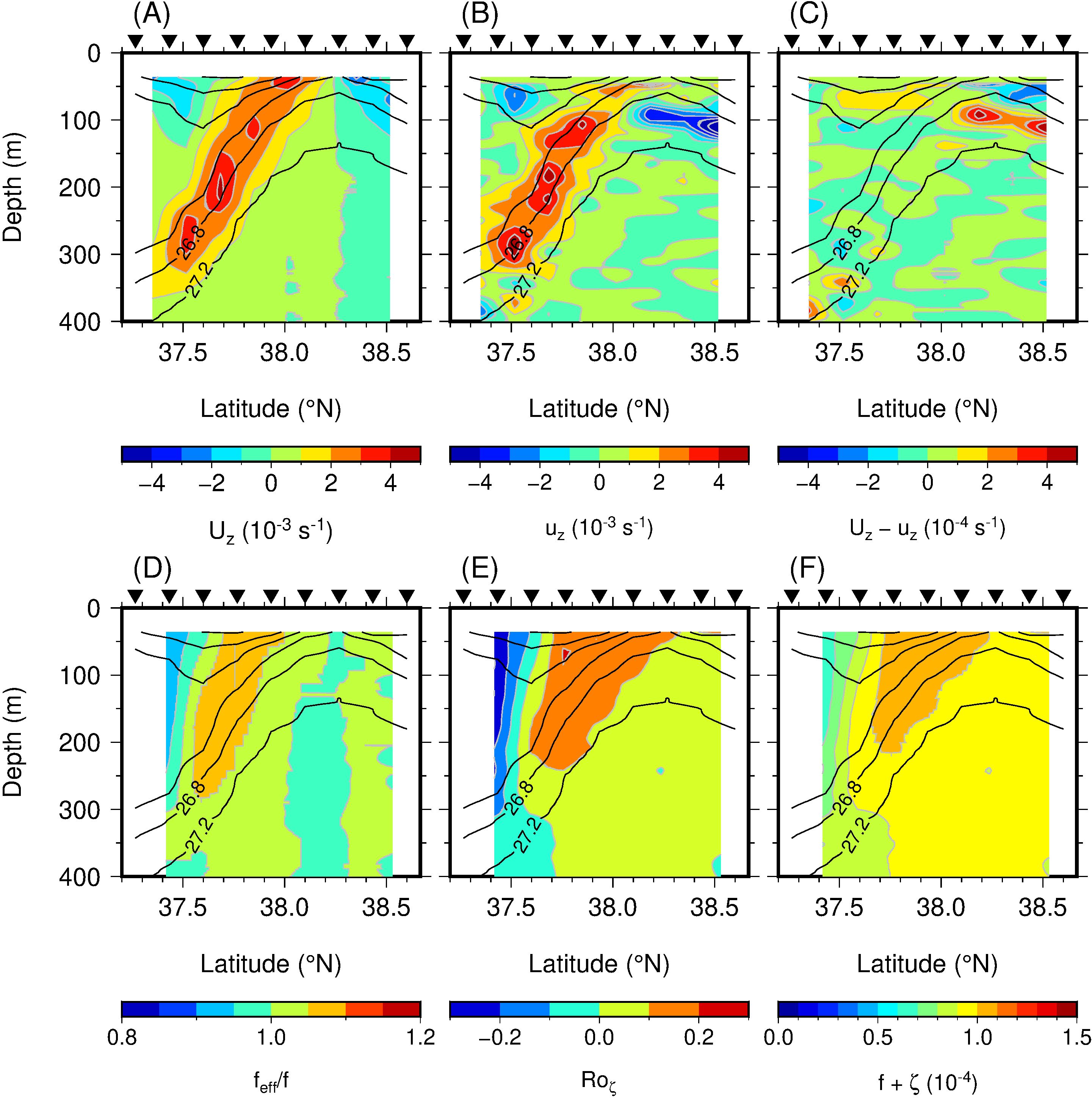
Figure 11. Sections of (A) U_z (s⁻¹), (B) u_z (s⁻¹), (C) U_z − u_z (s⁻¹) along the M3 transect. Sections of (D) f_eff normalized by f, (E) Ro_ζ, and (F) f + ζ (s⁻¹) between M2 and M3. Black inverted triangles at top of each panel indicate XCTD stations. Black lines denote σ_θ with a contour interval of 0.4 kg m⁻³ from 25.2 to 27.2 kg m⁻³.

The value of the effective Coriolis parameter in the zonal front, f_eff = f + u_y/2, normalized by f, was >1 near the front and<1 in the ACE (Figure 11D). In regions where the value of f_eff/f < 0, no significant values of ϵ and K_z were observed (Figures 9A, B, 10A, B). That is, the influence of near-inertial waves trapped by the ACE was not significant during the observation period. Equivalently, the observed values of ϵ were large in regions where the vorticity Rossby number (Ro_ζ = ζ/f = v_x – u_y) >0 (Figures 9A, B, 10A, B, 11E). The magnitude of Ro_ζ was ~0.2. While this value is not particularly large, it is sufficient to conclude that submesoscale phenomena could potentially be triggered. The condition Ro_ζ < 1 also supports the interpretation that the frontal sharpening stage was exponential (Hoskins and Bretherton, 1972). The quantity f + ζ, which is an indicator of submesoscale forced instabilities (i.e., inertial and symmetric instability; Thomas et al., 2013), was positive along the section (Figure 11F). Therefore, the influence of forced instability appears to be limited, thereby supporting the role of the ASC induced by the submesoscale frontogenesis in enhancing turbulent mixing.

The value of K_v, obtained under the assumption that the deformed flow balanced with the ASC (Equation 7), was large in regions of largely deformed flow and at the edges of these regions (Figures 12A, B). In regions where the value of K_v was large, the frontogenesis associated with the convergent flow is efficiently suppressed by the eddy viscosity. The distribution corresponded to that of K_z and K_θ; i.e., along transect M1 (Figure 12A): inside DB, around PA at a depth of 200 m around 38.1°N, and at depths of 150–200 m around 37.5°N within DA; and also along M2 (Figure 12B): within the ACE just south of the TWC front, and north of the front below DC at a depth of 300 m around 37.75°N. Along M2, large diffusion coefficients were observed north of DC by the VMP (Figure 10), whereas the value of K_v was estimated to be large south of the front because of the steeper velocity gradient. However, the distribution was similar to the observations in that the strong mixing was not found in areas of strong deformation with large density stratification associated with the front, but was found at their periphery. This distributional similarity supports to the interpretation that the observed turbulent mixing was enhanced by the ASC accompanying the frontogenesis. In addition, the distribution of K_v corresponds to that of the small ($⪅1$) value of the gradient Richardson number, Ri = b_z/(u_z²+v_z²) (Figure 12C), suggesting that the turbulent mixing was intensified in regions dominated by submesoscale and smaller-scale processes, where density stratification can be disrupted by velocity shear. These distribution is also consistent with the theory of ASC, which generates the vertical velocity on both sides of the front.

Figure 12

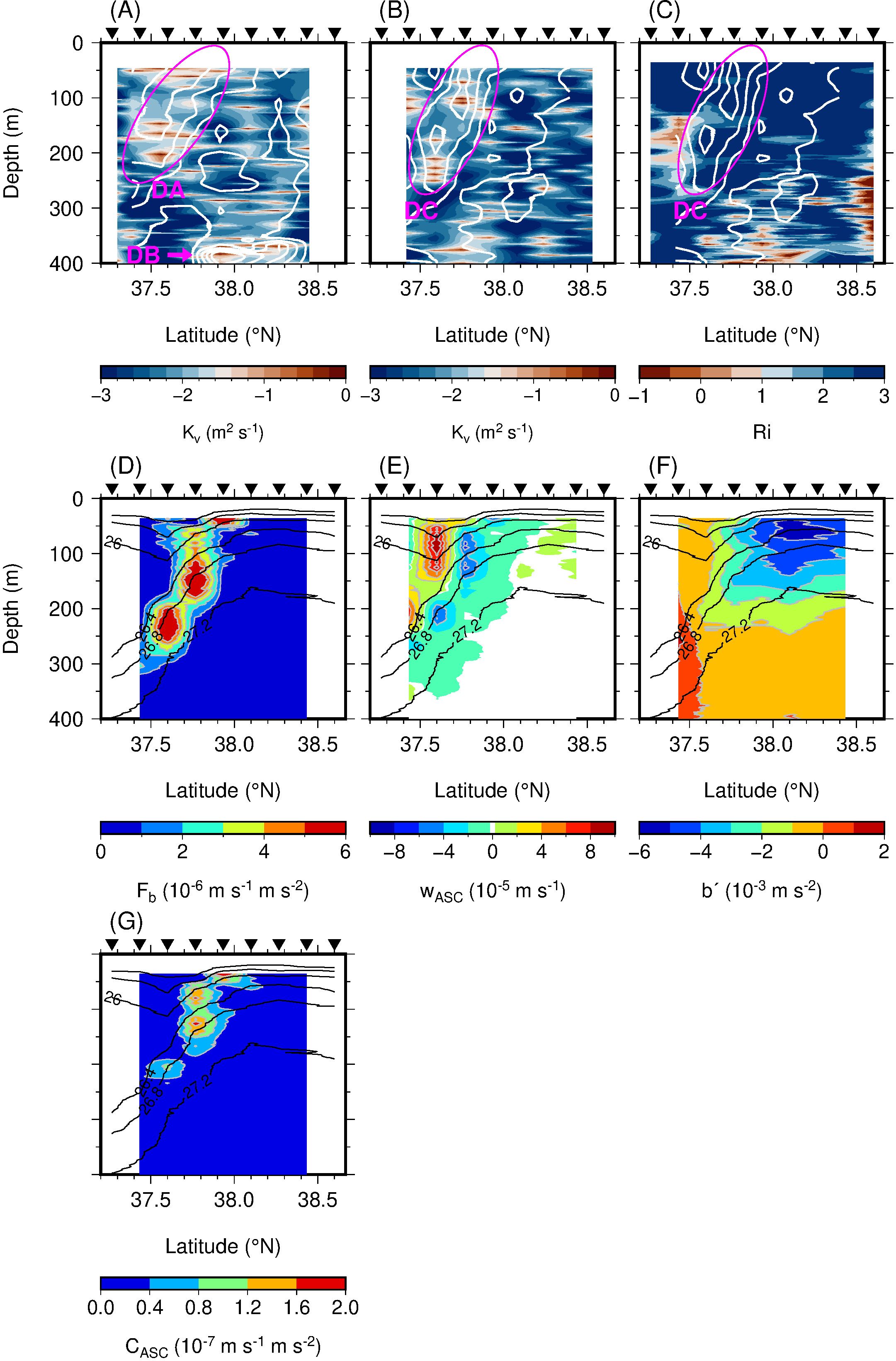
Figure 12. Sections of K_v (m² s⁻¹) along the (A) M1 and (B) M2 transects, (C) Ri along M2, (D) $F_b$ [m s⁻¹ m s⁻² (= W kg⁻¹)], (E) w_ASC (m s⁻¹), (F) b´ (m s⁻²), and (G) w_ASCb´ [m s⁻¹ m s⁻² (= W kg⁻¹)] between M2 and M3. Black inverted triangles at top of each panel indicate VMP and XCTD stations. White lines in (A–C) denote a/f with a contour interval of 0.05 from 0 to 0.3. Black lines in (D–G) denote σ_θ with a contour interval of 0.4 kg m⁻³ from 25.2 to 27.2 kg m⁻³.

The value of K_v was overestimated by two orders of magnitude (Figures 12A, B), probably because of our assumption that the deformation was completely offset by the frictional ASC. When only the frontogenesis driven by the deformation flow occurs, the vertical buoyancy flux associated with the ASC (Equation 8) showed large values near the front (Figure 12D). The integrated vertical buoyancy flux in the circulation cell (along transects M2–M3) was 2.0 × 10⁻³ W kg⁻¹ (Figure 13A). On the other hand, the integrated ϵ near the front along M2 (Figure 9B) was 1.9 × 10⁻⁵ W kg⁻¹ (Figure 13B). Therefore, if ~1% of the conversion from potential energy to kinetic energy that drives the ASC is efficiently used to generate the microscale turbulence, the observed turbulence can be explained (Figure 13). This observation and estimation demonstrate that the difference of two orders of magnitude was consistent with that between the observed diffusive coefficients (K_z and K_θ) and K_v estimated under the assumption that the deformation flow is frictionally balanced.

Figure 13

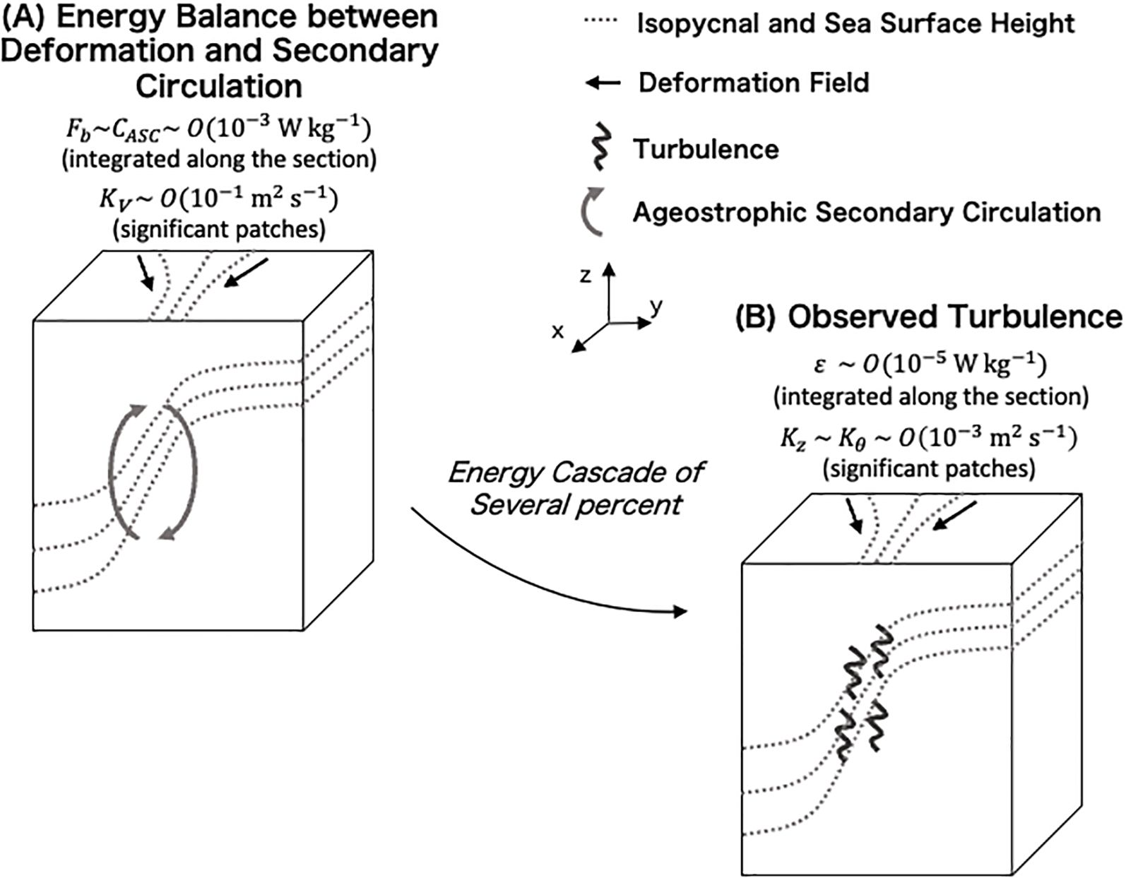
Figure 13. Stages and magnitudes of the energy flow based on our microstructure observations and energy balance estimation. Curved arrows between three-dimensional conceptual diagrams denote the expected energy flow. Broken lines denote isopycnals in the ocean interior and contours of sea surface height. Solid black arrows denote the deformation field. Gray arrows denote the ASC during frontogenesis.

The quantitative estimation of the vertical buoyancy flux (Equation 10) provides robust support for the verification of the closed energy loop. The distribution of w_ASC was consistent with the circulation pattern expected during frontogenesis (Figure 12E). The magnitudes were O(10⁻⁴ m s⁻¹) ~ O(10 m day⁻¹), exhibiting both positive and negative value. As a result of strong frontogenesis relative to M1 and M3, the cold water mass was prominently uplifted in the CE, leading to negative value of the difference between in situ buoyancy and the along-front mean buoyancy ($b\text{'}$) in the upper 200-m layer (Figure 12F). The buoyancy anomalies associated with the downward displacement of the warm water on the ACE side were also observed below 200 m around 37.5°N, but they were less pronounced than those caused by the uplift of cold water. The downward transport of the cold water caused by the ASC (Equation 9) resulted in enhanced energy conversion (C_ASC) on the CE side of the TWC front (Figure 12G). This distribution was similar to that of F_b estimated from the deformation flow and buoyancy gradient (Figure 12D), albeit with the magnitude one to two orders smaller (Figure 12G). The integrated value of the C_ASC along the section was 5.7 × 10⁻⁴ W kg⁻¹ (Figure 13A). Compared to the integrated ϵ value (1.9 × 10⁻⁵ W kg⁻¹; Figure 13B), it is evident that only a few (~3) percent of the ASC-supplied energy needs to cascade to turbulence. This closes the energy loop quantitatively.

4 Discussion

We used in situ observational data to investigate the process of submesoscale frontogenesis along the TWC front and the consequent enhancement of microscale turbulence. Multiple cross-sections captured deformation flow on the western side of the southward meander crest of the TWC front (Figures 5, 6). In particular, the convergent flow in the cross-front direction, and stretching in the along-front direction were significant. Forced by this deformation, the buoyancy gradient in the cross-front direction increased; i.e., frontogenesis occurred (Figure 7). Our high-density gridded observations allowed us to investigate the frontogenesis using these observational data, for which high-resolution reanalysis datasets have been used in previous studies (Ito et al., 2023). Several submesoscale patches of water mass were found near the growing front (Figures 3, 4). One of these was captured in multiple cross-sections and thus constituted the filament. The values of the turbulent dissipation rate and the vertical diffusion coefficients were large near the strong deformation flow and the patches (Figures 9, 10). The distribution of the velocity shear and physical parameters suggested that the contribution of the near-inertial waves with the turbulent mixing during the observation period was not significant.

The estimation of the vertical buoyancy flux and the resulted energy conversion revealed that only a few percent of the energy supplied by the ASC needs to cascade into turbulence to account for the observed turbulent dissipation (Figure 13). A substantial portion of the energy supplied from the available potential energy may be utilized for along-isopycnal horizontal advection, considering the expected scale of the motion (Figures 11E, 12C). The interaction between internal waves and forced submesoscale instabilities may be essential for facilitating more efficient mixing (Kawaguchi et al., 2020, 2021; McWilliams, 2016; Nagai et al., 2015; Srinivasa et al., 2019). The restricted energy flux from submesoscale to microscale dynamics may play a role in sustaining the seasonal mesoscale structures (Yabe et al., 2021) associated with the TWC. However, a more comprehensive assessment of the energy cascade resulting from submesoscale frontogenesis is necessary, including comparative studies with other major oceanic currents such as the Kuroshio, to better understand regional variability and underlying mechanisms.

As mentioned in the previous paragraph, the interaction of the submesoscale frontogenesis with the topography and internal waves should enhance further turbulent mixing. Observations over the southwestern end of the Yamato Ridge showed strong velocity shear (Figure 4) and associated enhancement of turbulent mixing (Figures 9, 10). Topographic wakes have been reported to form submesoscale eddies and enhance mixing due to the velocity shear caused by bottom friction on the bottom slope (McWilliams, 2016; Srinivasa et al., 2019). At the same time, although the survey suggested that the contribution of near-inertial waves to the turbulent mixing during the observation period was not significant (Figure 11), turbulent mixing can also be caused by the interaction between the frontogenesis and internal waves (Nagai et al., 2015). In addition, previous studies have demonstrated that near-inertial internal waves can be captured by anticyclonic mesoscale eddies (Kunze, 1985; Kunze et al., 1995), and then propagate downwards and dissipate into the turbulence there (Kawaguchi et al., 2020, 2021). In this study, we focused primarily on the relationship between the submesoscale phenomena associated with deformation flow and turbulent mixing, but future research should use in situ data to investigate the relationship between submesoscale phenomena triggered by the topography and turbulent mixing, as well as the mixing associated with the interaction between submesoscale phenomena and internal waves.

We expect that the deformation flow associated with the meandering of the flow observed in the TWC in this study would cause frontogenesis and enhance turbulent mixing over the global ocean. During August 2017, the Kuroshio began to follow the large meander path (Nagano et al., 2019, 2021; Qiu and Chen, 2021; Ito et al., 2024; Hirata et al., 2025), and this event is still on-going in spring 2025. Observations on the western side of the meander crest of the Kuroshio large meander (Ito et al., 2023) found frontogenesis and a resulting increase in nutrient supply from the lower to the subsurface layers and the concentration of the subsurface chlorophyll a maximum. The turbulent dissipation rate observed in this study was consistent with Ito et al.'s (2023) estimate of the nutrient supply from the lower layers associated with turbulent mixing in, supporting the influence of the frontogenesis and the resulting turbulent mixing on biological productivity in the meandering zone of the flow. Observations of a mesoscale eddy in the Kuroshio–Oyashio mixed water region (Ito et al., 2021) resulted in an estimate of around O(10⁻⁴ m² s⁻¹) for the vertical diffusion coefficient associated with the submesoscale spiciness patches found at the edge of the eddy, based on spiciness dissipation. This value is of the same order of magnitude as the K_θ associated with the low-S patch captured in this study (Figure 9). Using these analogies, the evaluation of the enhanced mixing and its contribution to biological productivity, and hence fisheries (Mahadevan, 2016), may be possible from the distribution of submesoscale patches, which are often observed in high-density observations. This study has demonstrated that both submesoscale frontogenesis and the resulting submesoscale water mass patterns contribute to turbulent mixing. We require a better understanding of the role of submesoscale frontogenesis, which is ubiquitous over the global ocean, and the resulting turbulent mixing.

Data availability statement

The raw data supporting the conclusions of this article will be made available by the authors, without undue reservation.

Author contributions

DI: Conceptualization, Data curation, Formal Analysis, Funding acquisition, Investigation, Methodology, Visualization, Writing – original draft, Writing – review & editing. YK: Conceptualization, Data curation, Investigation, Project administration, Resources, Writing – review & editing. TW: Data curation, Funding acquisition, Investigation, Project administration, Resources, Writing – review & editing. IY: Data curation, Investigation, Writing – review & editing.

Funding

The author(s) declare financial support was received for the research and/or publication of this article. This work was financially supported by JSPS KAKENHI (Grant number: JP22K03729; JP24H02227).

Acknowledgments

We thank the captains, officers, crew member, and scientists of the R/V Shinsei-maru cruise for their cooperation.

Conflict of interest

The authors declare that the research was conducted in the absence of any commercial or financial relationships that could be construed as a potential conflict of interest.

Generative AI statement

The author(s) declare that no Generative AI was used in the creation of this manuscript.

Any alternative text (alt text) provided alongside figures in this article has been generated by Frontiers with the support of artificial intelligence and reasonable efforts have been made to ensure accuracy, including review by the authors wherever possible. If you identify any issues, please contact us.

Publisher’s note

All claims expressed in this article are solely those of the authors and do not necessarily represent those of their affiliated organizations, or those of the publisher, the editors and the reviewers. Any product that may be evaluated in this article, or claim that may be made by its manufacturer, is not guaranteed or endorsed by the publisher.

References

Capet X., McWilliams J. C., Molemaker M. J., and Shchepetkin A. F. (2008a). Mesoscale to submesoscale transition in the California Current System. Part I: Flow structure, eddy flux, and observational tests. J. Phys. Oceanogr. 38, 29–43. doi: 10.1175/2007JPO3671.1

Crossref Full Text | Google Scholar

Capet X., McWilliams J. C., Molemaker M. J., and Shchepetkin A. F. (2008b). Mesoscale to submesoscale transition in the California Current System, Part II: Frontal Processes. J. Phys. Oceanogr. 38, 44–64. doi: 10.1175/2007JPO3672.1

Crossref Full Text | Google Scholar

Capet X., McWilliams J. C., Molemaker M. J., and Shchepetkin A. F. (2008c). Mesoscale to submesoscale transition in the California Current System. Part III: Energy balance and Flux. J. Phys. Oceanogr. 38, 2256–2269. doi: 10.1175/2008JPO3810.1

Crossref Full Text | Google Scholar

Chapman C. C., Sloyan B. M., Schaeffer A., Suthers I. M., and Pitt K. A. (2024). Offshore plankton blooms via mesoscale and sub-mesoscale interactions with a western boundary current. J. Geophys. Res.: Oceans. 129, e2023JC020547. doi: 10.1029/2023JC020547

Crossref Full Text | Google Scholar

Flament P. (2002). A state variable for characterizing water masses and their diffusive stability: Spiciness. Prog. Oceanogr. 54, 493–501. doi: 10.1016/S0079-6611(02)00065-4

Crossref Full Text | Google Scholar

Garrett C. J. R. and Loder W. (1981). Dynamical aspects of shallow sea fronts. Phil. Trans. R. Soc Lond. A. 302, 563–581. doi: 10.1098/rsta.1981.0183

Crossref Full Text | Google Scholar

Gula J., Molemaker M. J., and McWilliams J. C. (2014). Submesoscale cold filaments in the Gulf Stream. J. Phys. Oceanogr. 44, 2617–2643. doi: 10.1175/JPO-D-14-0029.1

Crossref Full Text | Google Scholar

Hales B., Hebert D., and Marra J. (2009). Turbulent supply of nutrients to phytoplankton at the New England shelf break front. J. Geophys. Res. 114, C05010. doi: 10.1029/2008JC005011

Crossref Full Text | Google Scholar

Hirata H., Nishikawa H., Usui N., Miyama T., Sugimoto S., Kusaka A., et al. (2025). The Kuroshio large meander and its various impacts: a review. J. Oceanogr. 81, 165–185. doi: 10.1007/s10872-025-00753-z

Crossref Full Text | Google Scholar

Hoskins B. J. (1982). The mathematical theory of frontogenesis. Ann. Rev. Fluid. Mech. 14, 131–151. doi: 10.1146/annurev.fl.14.010182.001023

Crossref Full Text | Google Scholar

Hoskins B. J. and Bretherton F. P. (1972). Atmospheric frontogenesis models: mathematical formulation and solution. J. Atmos. Sci. 29, 11–37. doi: 10.1175/1520-0469(1972)029<0011:AFMMFA>2.0.CO;2

Crossref Full Text | Google Scholar

Hoskins B. J., Draghici I., and Davies H. C. (1978). A new look at the ω-equation. Quart. J. R. Meteor. Soc 104, 21–38.

Google Scholar

Ichiye T. (1984). “Some problems of circulation and hydrography of the Japan Sea and the Tsushima Current,” in Ocean Hydrodynamics of the JAPAN and East CHINA Seas. Elsevier Oceanography Series. Ed. Ichiye T. (Amsterdam: Elsevier), 15–54.

Google Scholar

Igeta Y., Kumaki Y., Kitade Y., Senju T., Yamada H., Watanabe T., et al. (2009). Scattering of near-inertial internal waves along the Japanese coast of the Japan Sea. J. Geophys. Res. 114, C10002. doi: 10.1029/2009JC005305

Crossref Full Text | Google Scholar

Ito D., Kodama T., Shimizu Y., Setou T., Hidaka K., Ambe D., et al. (2023). Frontogenesis elevates the maximum chlorophyll a concentration at the subsurface near the Kuroshio during well-stratified seasons. J. Geophys. Res.: Oceans. 128 (5), e2022JC018940. doi: 10.1029/2022JC018940

Crossref Full Text | Google Scholar

Ito D., Shimizu Y., Setou T., Kusaka A., Ambe D., Hiroe Y., et al. (2024). Temporal variation of the 2017 Kuroshio large meander based on repeated surveys along 138°E. J. Oceanogr. 80, 1–21. doi: 10.1007/s10872-024-00718-8

Crossref Full Text | Google Scholar

Ito D., Suga T., Kouketsu S., Oka E., and Kawai Y. (2021). Spatiotemporal evolution of submesoscale filaments at the periphery of an anticyclonic mesoscale eddy north of the Kuroshio Extension. J. Oceanogr. 77, 763–780. doi: 10.1007/s10872-021-00607-4

Crossref Full Text | Google Scholar

Joyce T. M. (1989). On in situ “calibration” of shipboard ADCPs. J. Atmos. Oceanic Technol. 6(1), 169–172 doi: 10.1175/1520-0426(1989)006<0169:OISOSA>2.0.CO;2

Crossref Full Text | Google Scholar

Kaneko H., Yasuda I., Komatsu K., and Itoh S. (2012). Observations of the structure of turbulent mixing across the Kuroshio. Geophys. Res. Lett. 39, L15602. doi: 10.1029/2012GL052419

Crossref Full Text | Google Scholar

Kawabe M. (1982a). Branching of the Tsushima Current in the Japan Sea. Part I, data analysis. J. Oceanogr. Soc Jpn. 38, 95–102. doi: 10.1007/BF02110295

Crossref Full Text | Google Scholar

Kawabe M. (1982b). Branching of the Tsushima Current in the Japan Sea. Part II, numerical experiment. J. Oceanogr. Soc Jpn. 38, 183–192. doi: 10.1007/BF02111101

Crossref Full Text | Google Scholar

Kawaguchi Y. (2019). KS-19–22 cruise report, JAMSTEC. Available online at: http://www.godac.jamstec.go.jp/catalog/doc_catalog/metadataDisp/KS-19-22_all?lang=en (Accessed December 01, 2019).

Google Scholar

Kawaguchi Y., Wagawa T., and Igeta Y. (2020). Near-inertial internal waves and multiple-internal oscillations trapped by negative vorticity anomaly in the central Sea of Japan. Prog. Oceanogr. 181, 102240. doi: 10.1016/j.pocean.2019.102240

Crossref Full Text | Google Scholar

Kawaguchi Y., Wagawa T., Yabe I., Ito D., Senjyu T., Itoh S., et al. (2021). Mesoscale-dependent near-inertial internal waves and microscale turbulence in the Tsushima Warm Current. J. Oceanogr. 77, 155–171. doi: 10.1007/s10872-020-00583-1

Crossref Full Text | Google Scholar

Kawaguchi Y., Yabe I., Senjyu T., and Sakai A. (2023). Amplification of typhoon-generated near-inertial internal waves observed near the Tsushima oceanic front in the Sea of Japan. Sci. Rep. 13, 8387. doi: 10.1038/s41598-023-33813-9

PubMed Abstract | Crossref Full Text | Google Scholar

Klein P. and Lapeyre G. (2009). The oceanic vertical pump induced by mesoscale and submesoscale turbulence. Annu. Rev. Mar. Sci. 1, 351–375. doi: 10.1146/annurev.marine.010908.163704

PubMed Abstract | Crossref Full Text | Google Scholar

Kunze E. (1985). Near-inertial wave propagation in geostrophic shear. J. Phys. Oceanogr. 15, 544–565. doi: 10.1175/1520-0485(1985)015<0544:NIWPIG>2.0.CO;2

Crossref Full Text | Google Scholar

Kunze E., Schmitt R., and Toole M. J. (1995). The energy balance in a warm-core ring’s near inertial critical layer. J. Phys. Oceanogr. 25, 942–957. doi: 10.1175/1520-0485(1995)025<0942:TEBIAW>2.0.CO;2

Crossref Full Text | Google Scholar

Lapeyre G. and Klein P. (2006). Impact of the small-scale elongated filaments on the oceanic vertical pump. J. Mar. Res. 64, 835–851. doi: 10.1357/002224006779698369

Crossref Full Text | Google Scholar

Lévy M., Franks P. J. S., and Smith K. S. (2018). The role of submesoscale currents in structuring marine ecosystems. Nat. Commun. 9, 4758. doi: 10.1038/s41467-018-07059-3

PubMed Abstract | Crossref Full Text | Google Scholar

Mahadevan A. (2016). The impact of submesoscale physics on primary productivity of plankton. Annu. Rev. Mar. Sci. 8, 161–184. doi: 10.1146/annurev-marine-010814-015912

PubMed Abstract | Crossref Full Text | Google Scholar

Maúre E. R., Ishizaka J., Sukigara C., Mino Y., Aiki H., Matsuno T., et al. (2017). Mesoscale eddies control the timing of spring phytoplankton blooms: a case study in the Japan Sea. Geophys. Res. Lett. 44, 11115–11124. doi: 10.1002/2017GL074359

Crossref Full Text | Google Scholar

McWilliams J. C. (2008). Fluid dynamics at the margin of rotational control, Environ. Fluid. Mech. 8, 441–449. doi: 10.1007/s10652-008-9081-8

Crossref Full Text | Google Scholar

McWilliams J. C. (2016). Submesoscale currents in the ocean. Proc. R. Soc A. 472, 1–32. doi: 10.1098/rspa.2016.0117

PubMed Abstract | Crossref Full Text | Google Scholar

McWilliams J. C., Colas F., and Molemaker M. J. (2009). Cold filamentary intensification and oceanic surface convergence lines. Geophys. Res. Lett. 36, L18602. doi: 10.1029/2009GL039402

Crossref Full Text | Google Scholar

Mensa J. A., Garraffo Z., Griffa A., Özgökman T. M., Haza A., and Veneziani M. (2013). Seasonality of the submesoscale dynamics in the Gulf Stream region. Ocean. Dyn. 63, 923–941. doi: 10.1007/s10236-013-0633-1

Crossref Full Text | Google Scholar

Mori K., Matsuno T., and Senjyu T. (2005). Seasonal/spatial variations of the near-inertial oscillations in the deep water of the Japan Sea. J. Oceanogr. 61, 761–773. doi: 10.1007/s10872-005-0082-7

Crossref Full Text | Google Scholar

Morimoto A., Yanagi T., and Kaneko A. (2000). Eddy field in the Japan Sea derived from satellite altimetric data. J. Oceanogr. 56, 449–462. doi: 10.1023/A:1011184523983

Crossref Full Text | Google Scholar

Nagai T., Tandon A., Gruber N., and McWilliams J. C. (2008). Biological and physical impacts of ageostrophic frontal circulations driven by confluent flow and vertical mixing. Dyn. Atmos. Ocean. 45, 229–251. doi: 10.1016/j.dynatmoce.2007.12.001

Crossref Full Text | Google Scholar

Nagai T., Tandon A., Kunze E., and Mahadevan A. (2015). Spontaneous generation of near-inertial waves by the Kuroshio front. J. Phys. Oceanogr. 45, 2381–2406. doi: 10.1175/JPO-D-14-0086.1

Crossref Full Text | Google Scholar

Nagai T., Tandon A., Yamazaki H., and Doubell M. J. (2009). Evidence of enhanced turbulent dissipation in the frontogenetic Kuroshio Front thermocline. Geophys. Res. Lett. 36, L12609. doi: 10.1029/2009GL038832

Crossref Full Text | Google Scholar

Nagano A., Yamashita Y., Ariyoshi K., Hasegawa T., Matsumoto H., and Shinohara M. (2021). Seafloor pressure change excited at the northwest corner of the Shikoku Basin by the formation of the Kuroshio large-meander in September 2017. Front. Earth Sci. 8, 583481. doi: 10.3389/feart.2020.583481

Crossref Full Text | Google Scholar

Nagano A., Yamashita Y., Hasegawa T., Ariyoshi K., Matsumoto H., and Shinohara M. (2019). Characteristics of an atypical large-meander path of the Kuroshio current south of Japan formed in September 2017. Mar. Geophys. Res. 40, 525–539. doi: 10.1007/s11001-018-9372-5

Crossref Full Text | Google Scholar

Osborn T. R. (1980). Estimates of the local-rate of vertical diffusion from dissipation measurements. J. Phys. Oceanogr. 10, 83–89. doi: 10.1175/1520-0485(1980)010<0083:EOTLRO>2.0.CO;2

Crossref Full Text | Google Scholar

Qiu B. and Chen S. (2021). Revisit of the Occurrence of the Kuroshio large meander south of Japan. J. Phys. Oceanogr. 51, 3679–3694. doi: 10.1175/JPO-D-21-0167.1

Crossref Full Text | Google Scholar

Qiu B., Klein P., Sasaki H., and Sasai Y. (2014). Seasonal mesoscale and submesoscale eddy variability along the North Pacific Subtropical Countercurrent. J. Phys. Oceanogr. 44, 3079–3098. doi: 10.1175/JPO-D-14-0071.1

Crossref Full Text | Google Scholar

Qiu B., Nakano T., Chen S., and Klein P. (2017). Submesoscale transition from geostrophic flow to internal waves in the northwestern Pacific upper ocean. Nat. Commun. 8, 14055. doi: 10.1038/ncomms14055

PubMed Abstract | Crossref Full Text | Google Scholar

Sasaki H., Klein P., Qiu B., and Sasai Y. (2014). Impact of oceanic-scale interactions on the seasonal modulation of ocean dynamics by the atmosphere. Nat. Commun. 5, 5636. doi: 10.1038/ncomms6636

PubMed Abstract | Crossref Full Text | Google Scholar

Smith K. M., Hamlington P. E., and Fox-Kemper B. (2016). Effects of submesoscale turbulence on ocean tracers. J. Geophys. Res.: Oceans. 121, 908–933. doi: 10.1002/2015JC011089

Crossref Full Text | Google Scholar

Spall M. A. (1995). Frontogenesis, subduction, and cross-front exchange at upper ocean fronts. J. Geophys. Res. 100, 2543–2557. doi: 10.1029/94JC02860

Crossref Full Text | Google Scholar

Srinivasa K., McWilliams J. C., Molemaker M. J., and Barkan R. (2019). Submesoscale Vortical Wakes in the Lee of Topography. J. Phys. Oceanogr. 49, 1949–1971. doi: 10.1175/JPO-D-18-0042.1

Crossref Full Text | Google Scholar

Tandon A. and Nagai T. (2019). “Mixing associated with submesoscale processes,” in Encyclopedia of Ocean Science, 3rd edition, vol. 3 . Eds. Cochran J. K., Bokuniewicz J. H., and Yager L. P., 567–577. Amsterdam: Elsevier doi: 10.1016/B978-0-12-409548-9.10952-2

Crossref Full Text | Google Scholar

Thomas L. N. and Ferrari R. (2008). Friction, frontogenesis, and the stratification of the surface mixed layer. J. Phys. Oceanogr. 38, 2501–2518. doi: 10.1175/2008JPO3797.1

Crossref Full Text | Google Scholar

Thomas L. N., Tandon A., and Mahadevan A. (2008). Submesoscale processes and dynamics. Ocean. Modeling. an Eddying. Regime. Geophys. Monogr. Ser. 177, 17–38. doi: 10.1029/177GM04

Crossref Full Text | Google Scholar

Thomas L. N., Taylor J. R., Ferrari R., and Joyce T. M. (2013). Symmetric instability in the gulf stream. Deep-Sea. Res. 91, 96–110. doi: 10.1016/j.dsr2.2013.02.025

Crossref Full Text | Google Scholar

Thompson L. (2000). Ekman layers and two-dimensional frontogenesis in the upper ocean. J. Geophys. Res. 105, 6437–6451. doi: 10.1029/1999JC900336

Crossref Full Text | Google Scholar

Wagawa T., Kawaguchi Y., Igeta Y., Honda N., Okunishi T., and Yabe I. (2020). Detailed water properties of baroclinic jets and mesoscale eddies in the Sea of Japan from a glider. J. Mar. Syst. 201, 103242. doi: 10.1016/j.jmarsys.2019.103242

Crossref Full Text | Google Scholar

Wang D. P. (1993). Model of frontogenesis: Subduction and upwelling. J. Mar. Res. 51, 497–513. doi: 10.1357/0022240933224034

Crossref Full Text | Google Scholar

Yabe I., Kawaguchi Y., Wagawa T., and Fujio S. (2021). Anatomical study of Tsushima warm current system: Principal pathways and its variation. Prog. Oceanogr. 194, 102590. doi: 10.1016/j.pocean.2021.102590

Crossref Full Text | Google Scholar