Abstract
Affected by water level and rainfall, the failure probability of bank slope is of great time-dependent characteristics. Combining the random field theory with Monte Carlo simulation strategy to calculate long-term failure probability is a time-consuming when considering the spatial variability of geotechnical materials. Therefore, how to efficiently predict the long-term failure probability remains an urgent problem, which is vital to ensure the safety of bank slopes. This study combines remote sensing technology with machine learning methods to conduct comprehensive analysis on the long-term stability and failure probability of bank slope. Firstly, taking an actual bank slope as an example, the failure mechanism and time-dependent characteristics of it is studied with aid of the remote sensing technology. Subsequently, the stability of the bank slope within a year is quantified by the safety factor and seepage field obtained from the numerical model. The failure probability of the bank slope in the same year is calculated by the random field model, and the influence of uncertain parameters on the failure probability is drawn. Three deep learning models, such as multilayer perceptron, convolutional neural networks, and long short-term memory, are adopted to predict the long-term failure probability in 10 years. The results show that the failure probability increases with any of the uncertain parameters, such as the coefficient of variation, correlation coefficient of shear strength, or scale of fluctuation. The utilization of the novel method proposed by this study can efficiently depict the time-dependent characteristic of the long-term failure probability, and it is applicable in predicting the future failure probability of the bank slope. Among three models, the long short-term memory model shows better performance in predicting the time-dependent failure probability. The input data amount and the ratio of the training and test sets have an insignificant effect on the prediction results.
1 Introduction
The stability of coastal slope is vital to the safety of coastal engineering (Li et al., 2024; Li et al., 2025) such as the breakwater and embankments and etc. There are many external affecting factors especially the periodic wave loads and tidal water level variations leading to a time-dependent characteristics for deformation and stability of the coastal slope. The phenomenon is similar in bank slope which has been widely studied. As a result, studying the time-dependent characteristics of bank slope has reference significance on the safety of coastal slope.
With the construction of the Three Gorges Reservoir (TGR), many slopes nearby have become bank slopes. Due to changes in geological conditions and the surrounding environment, bank slopes will further evolve into reservoir bank landslides. For example, one of the greatest losses landslides the Qianjiangping landslide, the volume of the landslide body reaches 24 million m3, and the maximum surge generated by the landslide is 39 m, causing economic losses of approximately 80 million Chinese Yuan (Yin et al., 2015). The bedding slopes are the most common type in TGR. As the causing factors and conditions are different and complex for each landslide, the prevention and control of geological disasters caused by landslides in this area still face big challenges.
During the fluctuations of water level, the rock and soil mass in the sliding zone show an alternating dry and wet state. After being soaked and softened, the shear strength of the rock and soil decreases. This is an important condition for the revival of some ancient landslides or the multistep deformation and failure of reservoir bank landslides (Xu et al., 2020; Wu et al., 2023). By considering the dry-wet cycling effect of the sliding body and sliding zones of the Zhaoshuling landslide due to water level fluctuations, the variation of its stability under the reduction of the shear strength parameter of the slope body was analyzed (Zhang et al., 2022). Coupling the erosion and damage of the slope surface caused by rain, but the sliding zone had not yet reached saturation, Sun et al (Sun et al., 2023). used permeable boxes as the sliding surface and studied the effect of soil types in sliding zone on the revival of landslides by filling the permeable boxes with water. Su et al (Su et al., 2023). analyzed microscopic changes of sliding zone soil after interacting with acidic groundwater, normal groundwater, and distilled water environments and found that all three types of groundwater damaged the microstructure of the sliding zone soil to varying degrees. Among them, acidic groundwater had the most severe degree of damage to the soil structure. Zou et al (Zou et al., 2023). studied the mechanical properties of the sliding zone soil of the Liutang landslide through circum-shear tests and proposed a stability estimation method for landslides. This method was able to quantitatively express the relationship between the shear strength and displacement of the sliding zone soil under different moisture contents and normal stress states.
Rainfall is regarded as one of the important external factors causing landslides in the reservoir area (Yazdani et al., 2024; Zhang et al., 2024). Fan et al (Fan et al., 2020). generated a series of time series with different peak rainfall intensities and magnitudes. By comparing the dynamic characteristics of landslides induced by different rainfall patterns, they found that large early rainfall and uniform rainfall were the most probable patterns to cause landslides. Wang et al (Wang et al., 2021). classified the landslides caused by heavy rain into two failure modes. One was the sliding along the shear surface owing to the failure of the soil, and the other was the rapid sliding caused by the erosion of the slope. Yu et al (Yu et al., 2023). studied the failure of bedding slope containing interlayer soil under different rainfall patterns. They found that under uniform rainfall conditions, the rainfall threshold during landsliding would increase with the decrease of rainfall intensity. When there were peaks in the rainfall pattern, the rainfall threshold for landsliding was the smallest before the peak and the largest after the peak. A large number of the above-mentioned studies have shown that rainfall and reservoir water level are the main controlling factors when estimating the stability of reservoir bank landslides. Therefore, estimating the multistep deformation and evolution process of reservoir bank landslides, the effect of rainfall and reservoir water level, so-called the dynamic mechanical environment in this study, needs to be considered.
Reliability analysis quantifies the safety factor of geotechnical engineering from a probabilistic perspective, providing an effective way when considering the uncertainties of geotechnical engineering (Li et al., 2016; Jiang et al., 2022). It has been widely applied and developed in aspects such as uncertainty quantification (Li et al., 2019; Yang HQ. et al., 2021), advanced surrogate models (Li et al., 2023), and reliability design (Vagnon et al., 2020; Yang YJ. et al., 2021; Wang and Owens, 2022). Wu et al (Wu et al., 2017). conducted a reliability analysis and found that the reliability of the landslide gradually decreases as the strength of the sliding zone soil weakens. Zhang et al (Zhang et al., 2020). analyzed the changes in the failure probability of the Bazimen landslide under the dynamic mechanical environment based on monitoring data, and pointed out that the failure probability would increase with the increase of soil variability. Liao et al (Liao et al., 2021)further conducted dry-wet cycle tests to simulate the water level fluctuations on the Majiagou landslide. By analyzing the time-dependent reliability of the landslide for 10 years, they pointed out that the landslide would translate to an unstable state. Guardiani et al (Guardiani et al., 2022). adopted machine learning methods as surrogate models to study the relationship between the safety factor and time, and conducted sensitivity analyses on both the mechanical and hydraulic parameters. However, geotechnical parameters are usually regarded as random variables in the above-mentioned research, and existing research indicates that not considering spatial variability will lead to relatively conservative results (Huang et al., 2021; Li et al., 2022).
The spatial variability of geotechnical materials is always considered in numerical simulation under the basis on random field theory and Monte Carlo simulations. Considering the high cost and time-consuming calculation of MCS (Monte Carlo simulations), scholars have combined data-driven methods to construct surrogate models for achieving reliability analysis quickly and accurately. Wang and Goh (2021) used convolutional neural networks (CNNs) of which the predicting accuracy was very close to the results calculated directly using random fields, but the computational efficiency had been improved. Zhang et al (Zhang et al., 2023b). took the Bazimen landslide as an example and established the XGBoost and LightGBM prediction models to obtain the safety factor. The above-mentioned research verified the applicability of machine learning methods in improving efficiency in estimating the failure probability. However, for the reservoir bank landslides in dynamic mechanical environments, the failure probability of it is bound to show great time-dependent characteristics, and the long-term failure probability is of significant importance in estimating the risk of landslides. A novel method is needed to efficiently predict long-term reservoir bank landslide probability while accounting for soil and rock mass spatial variability.
This study, aiming at improving the prediction efficiency of the long-term failure probability of bank slope under the influence of dynamic mechanical environment, takes the Jiuxianping landslide in TGR as an example and proposes a novel method for the long-term failure probability prediction. To be specific, this paper is organized as follows. First, through the analysis of on-site geological and monitoring data, the failure mechanism and time-dependent displacement characteristics of the Jiuxianping landslide are determined. A numerical model of the landslide is established to assess its seepage field and safety factor in 2020. Subsequently, reliability analysis is performed using a random field model, incorporating the spatial variability of the sliding zone. Also, the effect of the uncertain parameters on failure probability is drawn. Finally, based on the 10-year failure probability from the random field model, a novel method for long-term failure probability prediction through deep learning is proposed and its high efficiency is verified. Furthermore, performance when using different deep learning models are compared and the effect of the data amount is discussed.
2 Stability evaluation of Jiuxianping landslide
2.1 Overview of landslide
The Jiuxianping landslide is a large wading landslide with a total volume of approximately 6902.5×104 m3. The distance between it and dam is 239 km. The center point coordinates are 108°4657.35” east longitude and 30°5627.63” north latitude. The average thickness of the landslide body is 40 m, and the area is about 174×104 m2. The bedding landslide with large-scale is shown in Figure 1. It is in a continuous deformation state, and once the landslide becomes unstable, it will cause incalculable losses.
Figure 1
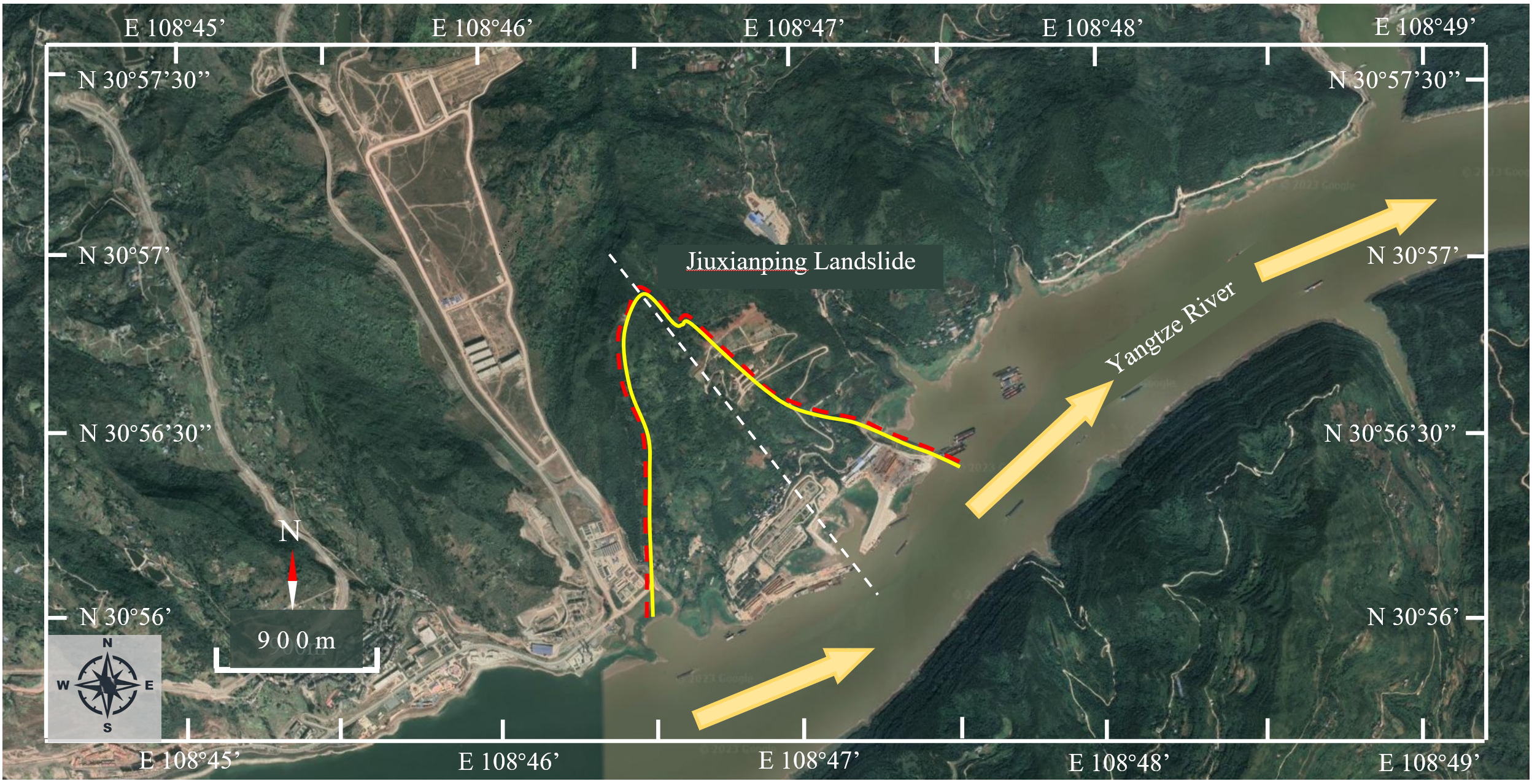
Location of Jiuxianping landslide.
Figure 2 plots the overall view of the Jiuxianping landslide, including the monitoring layout and actual view of the landslide. As plotted in Figure 2, the rear edge of the Jiuxianping landslide shows obvious signs of sliding. The middle of the slope is relatively straight, while the front part is characterized by steep cliffs and slopes. The overall failure mechanism of the Jiuxianping landslide is sliding-bending. To be specific, the shallow, fragmented rock masses are sliding locally while the rear accumulation body is sliding along the bedrock surface in a pushing manner. Because the Jiuxianping landslide is a bedding slope, the dip angle of the rock strata is greater than the gradient of the slope. Under the circumstance that the dip angle of the sliding surface is greater than the friction angle of that surface, landslide occurs However, there still exists a resistance for the rock mass to slide, and this makes the rock mass in the middle and lower parts bend and deform until it leads to collapse and failure. Therefore, the development of the landslide can be divided into three stages: the slightly bended stage, the strongly bended and uplifted stage, and the slide surface formed stage. Owing to the release of energy developed in the first 2 stages, the landslide accelerates with additional thrust.
Figure 2
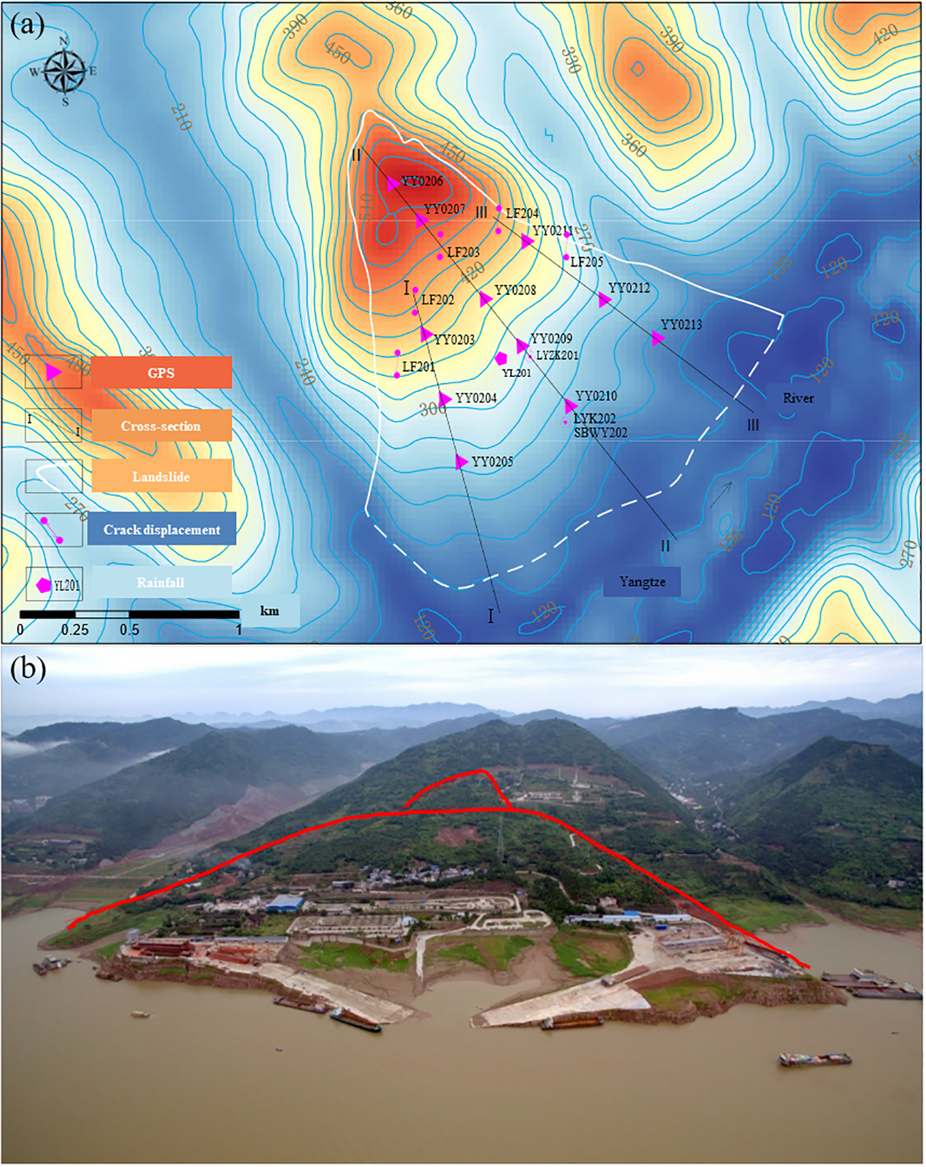
Overall view of Jiuxianping landslide: (A) monitoring layout; (B) actual view.
2.2 Measured data
This section exhibits the measured data from the global navigation satellite system (GNSS) for which the monitoring layout is shown in Figure 2A. Figures 3 and 4 plot the cumulative displacement and deformation rate with time, as well as the corresponding water level and rainfall from June 2016 to November 2021.
Figure 3
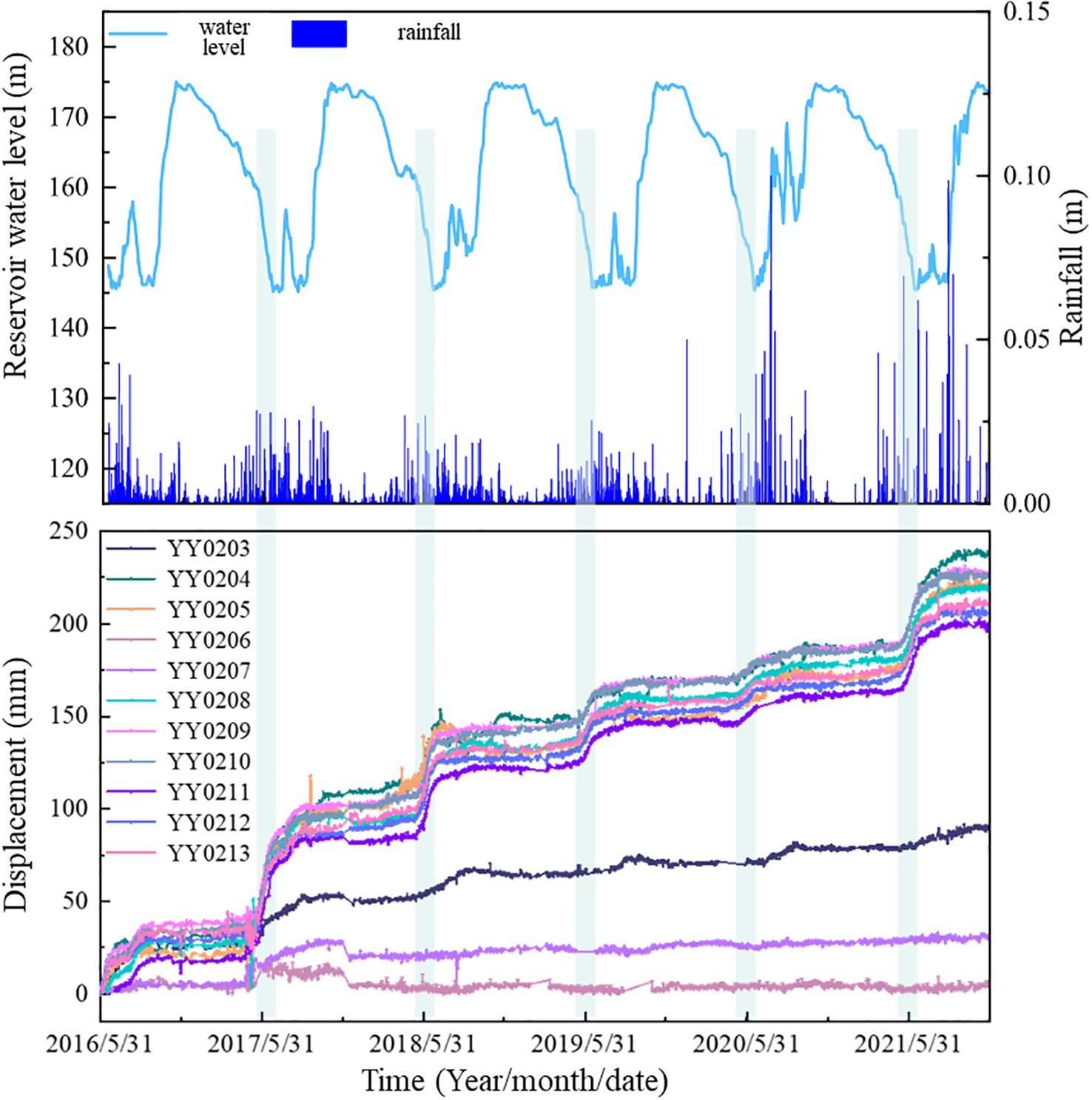
Monitored displacement of Jiuxianping landslide.
Figure 4
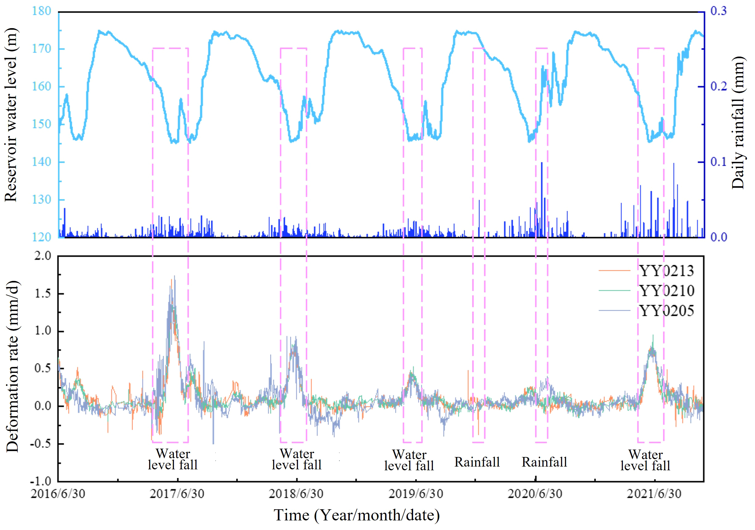
Variation of deformation rate with reservoir water level and rainfall.
The Jiuxianping landslide’s deformation primarily occurs at the middle and leading-edge sections. The displacement trends at multiple monitoring points in the middle and leading-edge areas are consistent, suggesting the entire landslide is sliding downward. From 2016 to 2021, the cumulative horizontal displacement of the middle and leading edge of the Jiuxianping landslide reached 237.5 mm. The change of displacement was the greatest in 2017, with an increment of approximately 66.3 mm. The cumulative horizontal displacement at the rear edge was relatively small (i.e., 55.9 mm), and the increment within 2021 was approximately 5.7 mm.
The cumulative displacement curve shows a stepped pattern, reflecting intermittent sharp increases followed by slower deformation periods. Further observation of the deformation rate of the middle and leading-edge positions reveals that the displacement shows a great time-dependent characteristic. The displacement shows regular changes. Take the data of 2021 as an example. From January to April, the deformation rate of each monitoring point was relatively low at 1mm/month. From May to October, the deformation rate increased sharply, with the deformation rate being around 2.0~8.2 mm/month. From November to December, the deformation rate decreased to 1 mm/month.
Compared with the corresponding reservoir water level and rainfall data, these two factors are the most important affecting landslide deformation. Displacement peaks annually in June (with deformation rate reaching 1.9 mm/day) during flood season water level fluctuations (see Figures 3, 4). In other months, the reservoir water level was increased or at a high water level, and the landslide did not show obvious deformation. Water level decline creates an outward hydrodynamic pressure (higher inner/outer head difference) at the landslide front, reducing slope stability.
With the influence of rainfall in the flood season, the landslide displacement shows a stepwise deformation. On the one hand, rainwater seeps into the slope, increasing the gravity of the sliding body and thus the sliding force. On the other hand, the softening effect of landslide soil lowers the resistance of the slope and leads to the instability of the landslide. However, the impact of rainfall individually is smaller than water level. Even at 0.1 m/d rainfall inducing 0.25 mm/d landslide displacement, the movement remains smaller than during reservoir drawdown.
2.3 Numerical model
To quantitatively evaluate the stability of the landslide, the numerical model (Zheng et al., 2025a; Zheng et al., 2025b) of the Jiuxianping landslide is established in Slide 2. Based on the Morgenstern-Price method, the safety factor Fs is calculated, and the mechanism of interaction between reservoir water level and rainfall is investigated in combination with the theories of unsaturated seepage and unsaturated shear strength. The typical cross-section of the Jiuxianping landslide is selected within a hydrological year. When conducting the steady-state seepage calculation, the constant-head boundary is prescribed at the leading edge with 175 m and the below area, and the water head on the left side is set as 360 m according to the monitoring data. For transient seepage analysis, a variable-head boundary (145~175 m) matching the Yangtze River’s actual water level is prescribed at the leading edge. The remaining areas of the slope are set as rainfall flux boundaries, consistent with the monitored daily rainfall. The numerical model is divided by using three-node triangular meshes, with a total of 3,273 meshes. Since the sliding zone has been identified, the sliding surface in the simulation is completely specified.
In the typical cross-section, strata are formed by silted clay containing crushed stones, fractured rock mass, sliding zone, and bedrock, as shown in Figure 5. The geotechnical parameters for the typical strata are listed by conducting the laboratory tests in Table 1. Mohr-Coulomb criteria are adopted in the model. Based on the Slide 2 seepage analysis module, the van-Genuchten empirical model is used to obtain the soil-water characteristic curves and permeability functions.
Figure 5
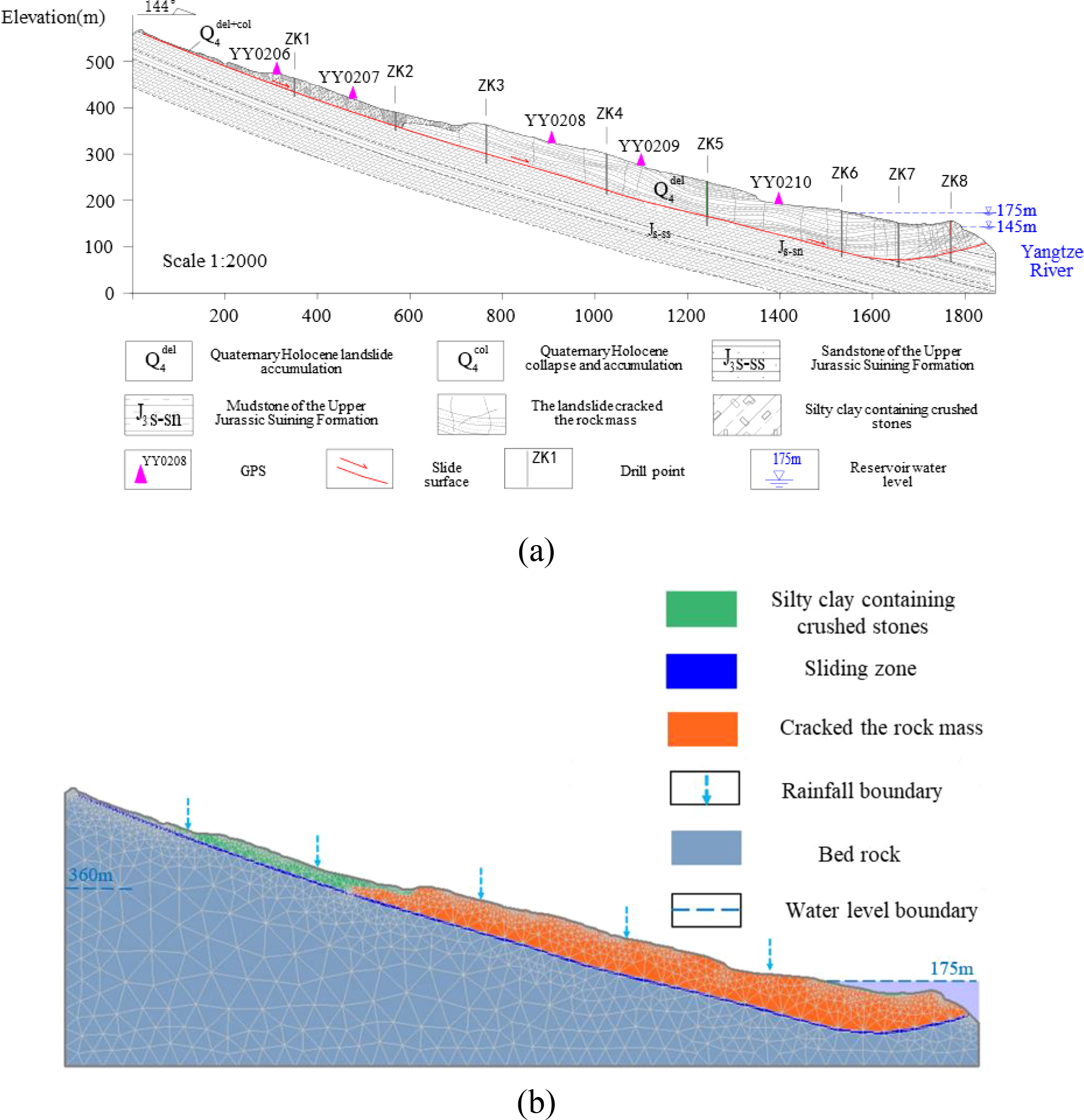
Typical profile of Jiuxianping landslide: (A) Geological profile; (B) Generalized model.
Table 1
| Soil layer | Unit weight (kN/m3) | Cohesion (kPa) | Friction angle (°) | Permeability (m/s) | Saturation moisture content | Residual moisture content |
|---|---|---|---|---|---|---|
| Silted clay containing crushed stones | 20.9 | 27 | 21.38 | 3.2×10⁻⁶ | 0.35 | 0.03 |
| Fractured rock mass | 24.9 | 840 | 28 | 2.78×10⁻⁶ | 0.25 | 0.03 |
| Sliding zone | 19.11 | 12.5 | 15 | 5.42×10⁻⁶ | 0.35 | 0.05 |
| Bedrock | 25.2 | 6200 | 42.3 | 1×10⁻⁸ | 0.0844 | 0.015 |
Rock and soil parameters of Jiuxianping landslide.
2.4 Stability evaluation
In 2020, the TGR faced its largest flood peak (i.e., 75,000 m³/s) during the No. 5 flood event in July-August which is the highest since the reservoir’s operation began. Therefore, stability evaluation is carried out based on the condition in 2020. Figures 6, 7 show the variation of seepage field and Fs in 2020.
Figure 6
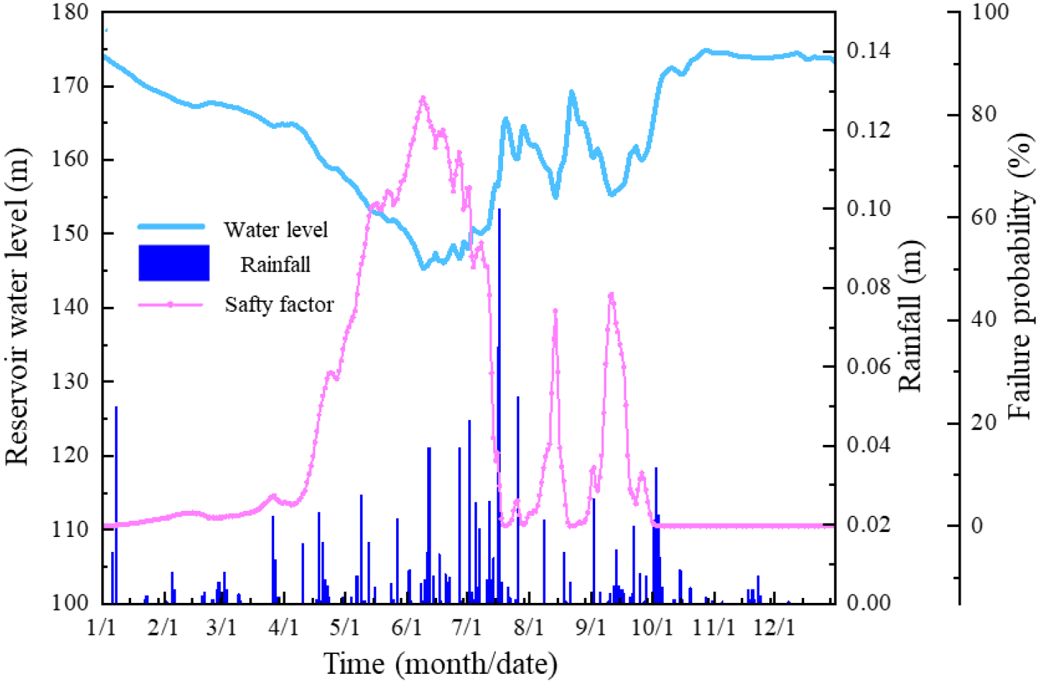
Variation of Fs in the whole 2020.
Figure 7
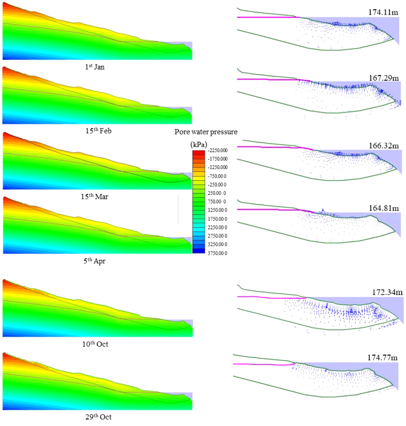
Variation of the seepage field.
As shown in the Figure 6, the water level experienced great decline and increase in the duration from January to April and from June to September. It is easy to find that Fs shows a positive correlation with reservoir water level. Both the variation trend and the varying rate are consistent between Fs and the reservoir water level. Furthermore, affected by rainfall, Fs reaches the minimum value 1.189 in June. Compared to the reservoir water level, rainfall has a more irregular and subtle effect on landslide behavior.
Combined with the seepage field shown in Figure 7, it can be observed that the infiltration line at the leading edge of the landslide becomes upward convex shape and upward concave shape (e.g., on April 5th and October 29th) when water level declined and increased. A faster-changing water level makes the phenomenon more noticeable. This occurs because the rate of change in the reservoir water level exceeds the slope’s permeability coefficient, resulting in a lag effect of the infiltration line in slope. Also, this is the failure mechanism of landslide affected by reservoir water level. When the infiltration line becomes upward convex shape, the outward seepage-induced water pressure reduces slope stability, triggering landslide movement. On the contrary, the slope is stable.
After October 24th, the water level increased to 174.04m and then began to operate at a high level. On October 29th, Fs of the landslide reached its peak (i.e., 1.274). Following this, the reservoir water level did not change significantly, but Fs slightly decreased. This phenomenon results from the reduction and eventual dissipation of the hydraulic head gradient across the slope interface. That means the infiltration pressure towards the slope is gradually disappearing. Fs shows a slightly decreasing trend due to the floating effect brought by the reservoir water.
3 Reliability analysis considering the variability of sliding zones
3.1 Establishment of the RFM
Stochastic analysis is conducted in this section to further obtain the failure probability of the landslide. To consider the spatial variability of geotechnical materials, the Local average subdivision method is adopted to expand the random field. Based on the local average theory, the accuracy is achieved through the continuous subdivision of elements. The Markovian autocorrelation function is adopted shown as Equation 1.
where and represent the horizontal and vertical scale of fluctuation, respectively; and represent the horizontal and vertical distances between two points. Stochastic analysis is carried out by combining the Monte-Carlo Simulation (MCS) strategy with Latin-hypercube-sampling (LHS).
To reflect the uncertainty of the slide zone, the mean μ and standard deviation σ of the shear strength parameters are obtained according to the onsite borehole data. Statistical analysis shows the sliding zones’ shear strength follows a lognormal distribution. Referring to the literature of similar bedding landslides in the TGR (Li et al., 2015; Zhang et al., 2023a), lx is in a range of 20–80 m, while ly is in a range of 2–6 m. As a result, the spatial variability parameters are determined in Table 2.
Table 2
| Parameters | μ | σ | Scale of fluctuation | Correlation coefficient | Distribution |
|---|---|---|---|---|---|
| Cohesion (kPa) | 12.5 | 0.3 | lx=20m ly=2m | -0.5 | Lognormal |
| Friction angle (°) | 15 | 0.2 |
Statistical properties of the sliding zone.
Figure 8 shows one of the implementations of the random field. In the software, the grid is automatically divided by the software based on the input variability parameters and the Markov autocorrelation function. The grid size is at least half of the lx or ly, and each material layer has a sufficient number of grids to correctly represent the spatial variability. A total of 5,000 implementations is conducted in every stochastic case. As shown in Figure 9, both the μ and σ of Fs exhibit stabilizing tendencies when the implementation time is 5000, indicating that the probability analysis results can meet the accuracy requirements.
Figure 8
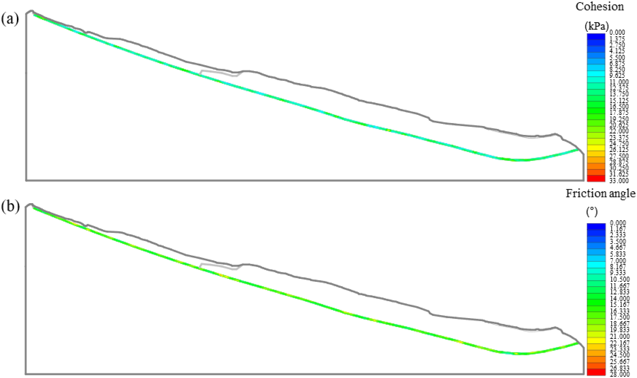
Random field for (A)c and (B)φ.
Figure 9
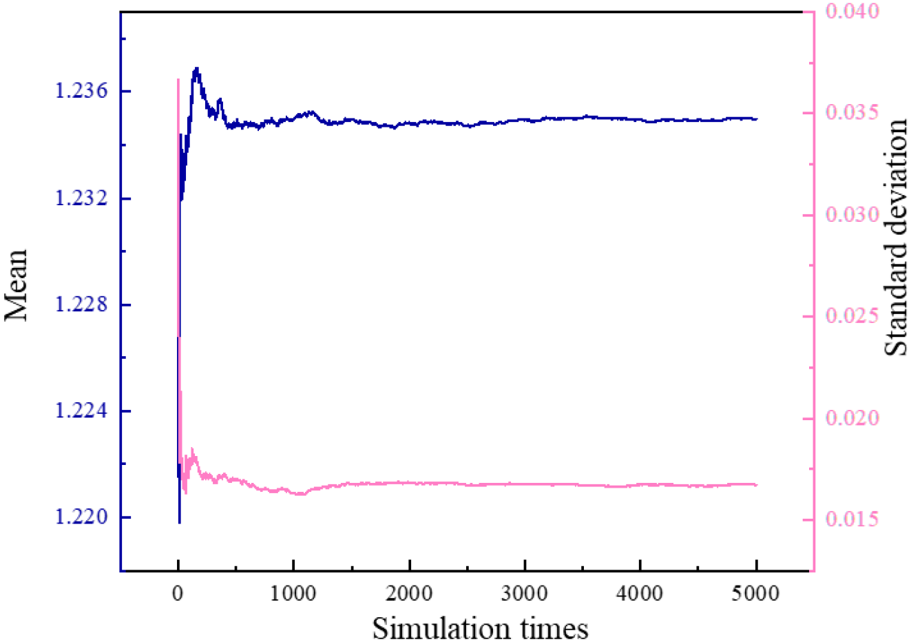
Variation of μ and σ of Fs with MCS simulation times.
3.2 Reliability analysis
Referring to the “Technical requirements for engineering geological investigation of geological hazard prevention in TGR (Three Gorges Reservoir Area Geological Hazard Prevention Headquarters, 2014), simulation cases with Fs less than 1.2 are considered unstable. Also, the reliability analysis is conducted according to the time stage clarified in the Table 2.
Figure 10 demonstrates the variation of failure probability (Pf) during each time stage and the whole of 2020. According to Figure 10A, Pf in stage 1 is relatively small, ranging from 0 to 5.9%. As the reservoir water level declines more obviously in stage 2 (see Figure 10B), Pf increases sharply, with a maximum reaching 83.32%. Seeing from Figure 10C, as the water level went through a quick increase and decline, so does the variation of Pf. From June 10th to July 21st, the water level increased, and Pf decreased sharply from 81.96% to 0.22%. On August 14th, as the water level declined to its lowest, Pf increased to 41.82%. During August and September, Pf decreased to 0 and then increased to 44.72% with a water level increase first and decline. According to Figures 10D, E, the water level increased from 155.28m to 172.34m at stage 4, and the water level stayed at a high level at stage 5. From September 23rd to September 26th, the reservoir water level declined slightly, Pf decreased from 45.06% to 0. After that, Pf stays 0.
Figure 10
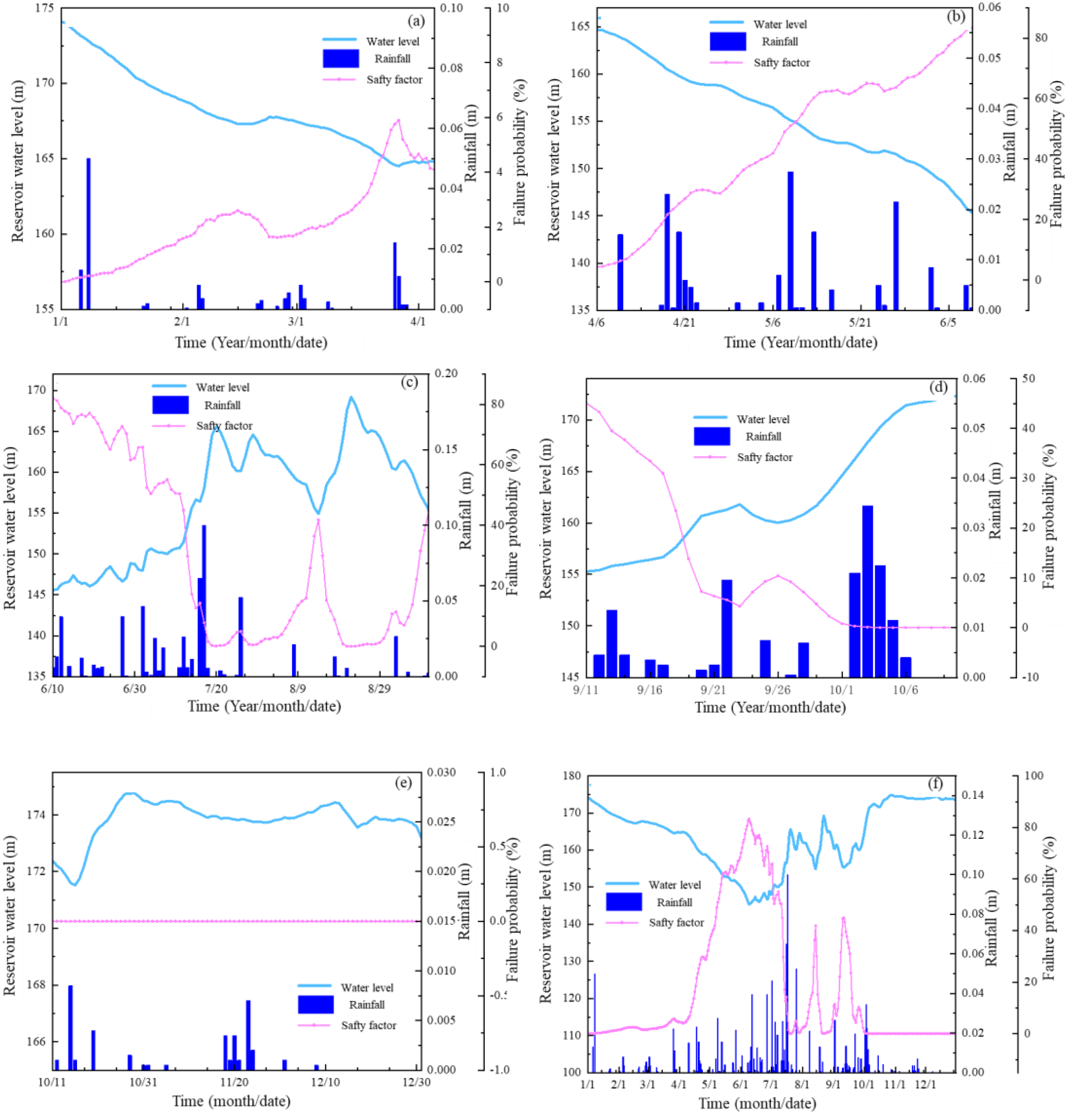
Failure probability at stages 1~5 (A–E) and the whole 2020 (F).
Figure 10F demonstrates the variation of Pf in the whole year. Compared with the deterministic analysis in section 2.4, the variation pattern of Pf demonstrates remarkable consistency with deterministic evaluation results. However, the response of Pf is more intense. In other words, the reliability analysis can provide early warning of reservoir bank landslides.
3.3 Parametric analysis
3.3.1 Coefficient of variation
To study how the variation in c and φ of the sliding zone affects Pf, the heaviest rainfall day in the 2020 flood season (July 11th, with 0.1m of rainfall) is selected as the study case. The variation of Pf with COVc and COVφ is plotted in Figure 11. Pf increases from 7.76% to 8.04% when COVc increases from 0.05 to 0.4. Pf increases from 0 to 35.96% when COVφ increases from 0.05 to 0.4, with a relatively large variation range. When COVc and COVφ increase, Pf increases simultaneously. However, compared with the influence of COVφ, COVc has a relatively small effect on Pf.
Figure 11
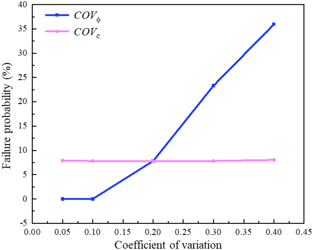
Failure probability with different COVc and COVφ.
To further investigate the effect of COVφ, the probability density curve and cumulative distribution curve of Fs for different COVφ are drawn in Figure 12. As shown in Figure 12, the shape of the curves changes a lot when COVφ varies, and this is the main reason that Pf is sensitive to COVφ. When COVφ is as small as 0.05, the probability density curve shape is steep and presented as a concentrated distribution. With the increase of COVφ, the peak value decreases and gradually shifts towards the left, and the curve shape becomes short and wide, indicating a more unstable and uncertain condition for the landslide. As for the cumulative distribution of Fs, these curves intersect at one point at which Fs is about 1.23. When COVφ increases, the slope of the curve decreases when Fs is smaller than 1.23 but increases when Fs is larger than 1.23. That is to say, the frequency for smaller Fs also increases, showing a more unstable condition of landslide.
Figure 12
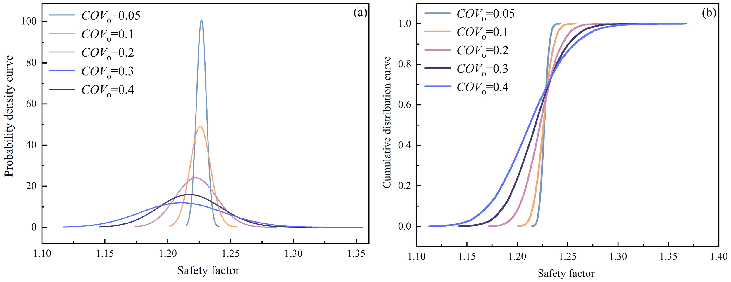
Influence of coefficient of variation: (A) Probability density curve of friction angle; (B) Cumulative distribution curve of friction angle.
3.3.2 Correlation coefficient
Figure 13 shows the effect of the correlation coefficient of c and φ on Pf. When the correlation coefficient changes from -0.7 to 0.5, Pf increases from 7.32% to 9.22%. This indicates that, compared with the negatively correlated, positively correlated c and φ are more unfavorable for the stability of the landslide. However, Pf is not that sensitive to the correlation coefficient, as the variation range is not that large. The probability density curve and cumulative distribution curve of the Fs with different correlation coefficients are drawn in Figure 14. With different correlation coefficient, the shape of the probability density curves remains almost the same, and the peak value increases slightly. The cumulative distribution curves almost coincide with each other.
Figure 13
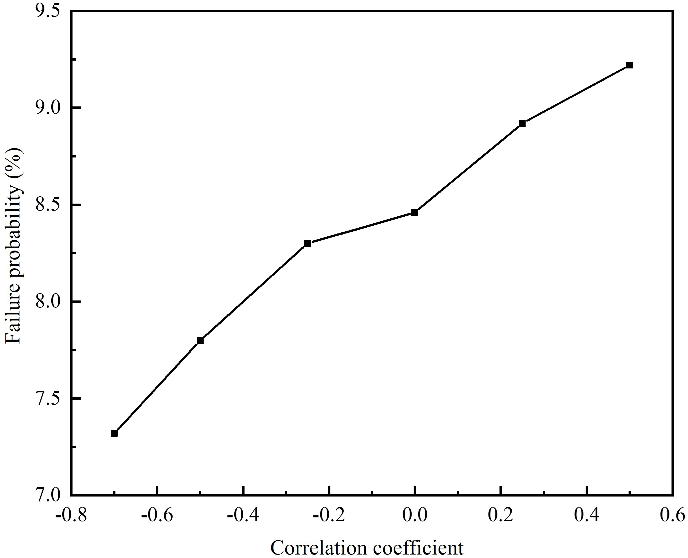
Failure probability with different correlation coefficient.
Figure 14
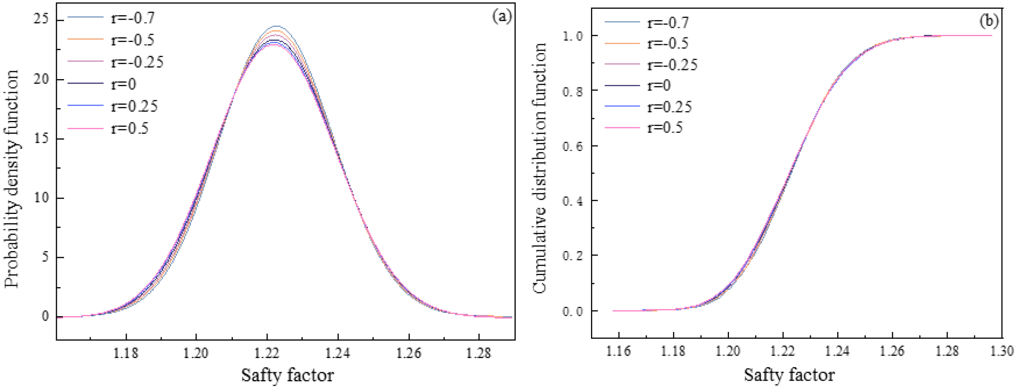
The influence of different correlation coefficients: (A) Probability density curve; (B) Cumulative distribution curve.
3.3.2 Scale of fluctuation
To compare the vertical and horizontal scale of fluctuation together, define the coefficient for scale of fluctuation as the ratio of lx or ly between the case and the basis case mentioned in the Table 3. Figure 15 shows Pf with lx or ly. Pf increases with both lx and ly, but to different extents. As lx increases from 10m to 60m, Pf increases from 5.42% to 11.32%. As ly increases from 1m to 6m, Pf increases from 4.26% to 10.1%. When the lx or ly is large enough, the stochastic field representation reduces to a random variable formulation. This also indicates that the random variable model can obtain a conservative result of Pf. The probability density curve and cumulative distribution curve of the Fs with different lx are drawn in Figure 16. As lx increases, the peak of its probability density curve gradually decreases, and the distribution becomes more extensive. The overall shape evolves from a tall and narrow type to a short and wide type, and the slope of the cumulative distribution function curve gradually becomes flatter. The failure probability of the landslide will also increase accordingly.
Table 3
| Model | R2 | MAE | RMSE | |||
|---|---|---|---|---|---|---|
| Training set | Test set | Training set | Test set | Training set | Test set | |
| MLP | 0.9900 | 0.9741 | 1.50 | 2.25 | 2.90 | 4.48 |
| CNN | 0.9932 | 0.9784 | 1.16 | 2.03 | 2.40 | 4.09 |
| LSTM | 0.9932 | 0.9823 | 1.06 | 1.72 | 2.39 | 3.70 |
Evaluation index of three models.
Figure 15
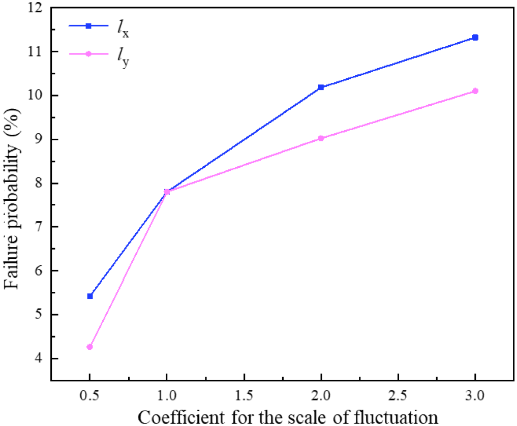
Failure probability in different scale of fluctuation.
Figure 16
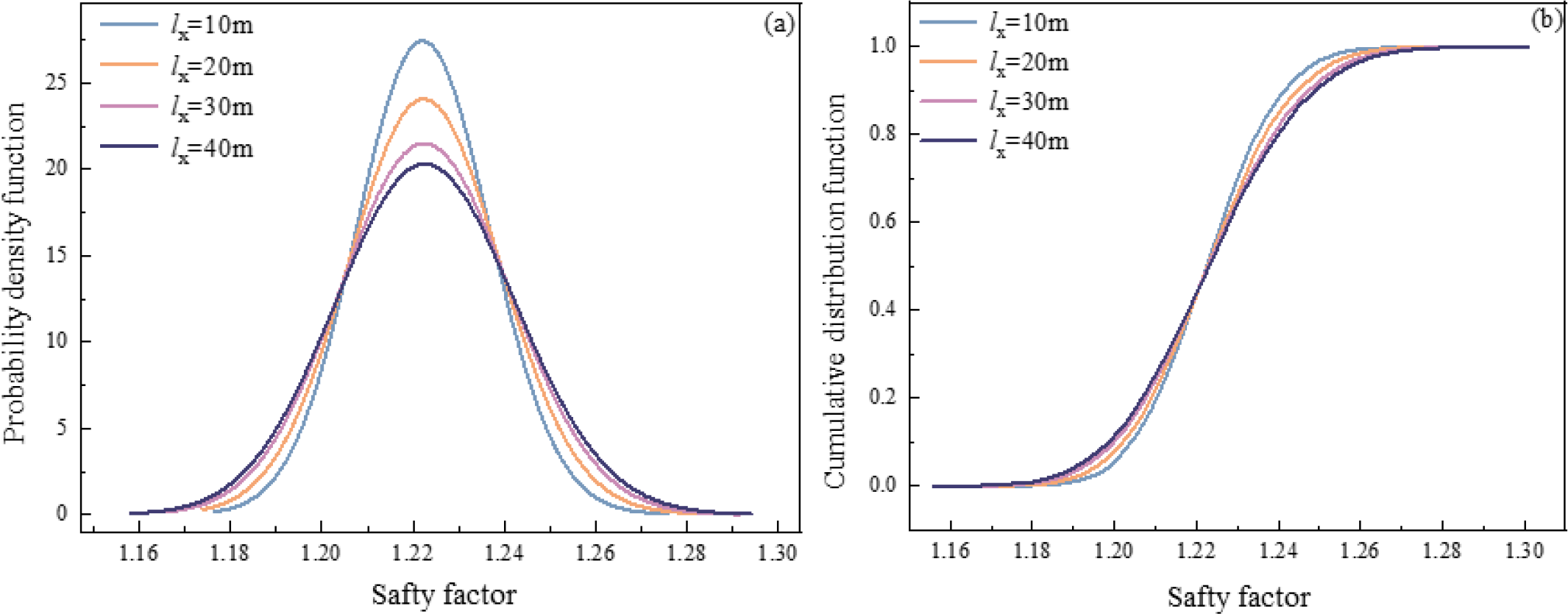
. The influence of different scale of fluctuation: (A) probability density curve; (B) cumulative distribution curve.
4 Time-dependent failure probability prediction
Due to the high time cost when using MCS, surrogate models are widely used in reliability analysis. Nevertheless, their predictive accuracy requires further enhancement, and these models can not reflect the time-dependent characteristic of the predicted scope. As has been analyzed above, the displacement, stability, and Pf of the Jiuxianping landslide show very intense time-dependent characteristics affected by reservoir water level and rainfall. Therefore, this study proposes a novel method based on deep learning that has been successfully applied in time series prediction in stochastic analysis, and attempts to predict the temporal evolution of Pf. Through the time series prediction, Pf at future time points and long-term reliability evaluation can be further obtained.
4.1 Methodology
4.1.1 Multilayer perceptron
Single-layer neural networks require linear separability, but adding more neurons between the input and output layers can solve nonlinear separation problems. The Multilayer Perceptron (MLP), a simple yet powerful deep learning model, acts as a mapping function. MLP can approximate arbitrary nonlinear functions, making them highly effective for time series prediction.
4.1.2 Convolutional neural networks
CNN uses convolutional layers to extract features via sliding kernels, ensuring translation invariance—detecting features regardless of their position. Pooling layers (e.g., max/average pooling) down sample these features, expanding the kernel’s receptive field to capture broader patterns. Finally, a fully connected layer integrates all features for classification or recognition. Though designed for images, CNN can also outperform recurrent neural networks (RNN) in certain sequence tasks while being computationally cheaper.
4.1.3 Long short-term memory
Unlike standard RNNs, LSTM introduces a cell state Ct and three gating mechanisms to control information flow. The forget gate determines the content to be forgotten from Ct-1 using a sigmoid-activated output ft. The input gate determines which new information to store in the cell state via sigmoid (it) and tanh t layers. The output gate regulates the next hidden state ht by filtering the updated cell state Ct through a sigmoid ot and tanh layer. By selectively retaining or discarding information at each step, LSTM effectively captures long-range temporal dependencies, and it is a key advantage over traditional RNN in tasks like time-series prediction.
4.2 Preparation of data
Pf of the landslide during 2011–2020 is calculated according to the numerical method mentioned in section 3, and the results are demonstrated in Figure 17. The deep learning models are established using the TensorFlow framework. The dataset is partitioned into training and test sets with a 7:3 ratio. The data involving 2011–2017 and 2018–2020 are regarded as the training set and test set, with a data amount of 2558 and 1095, respectively. Taking the current day as the starting point, the model is trained using the data of the previous five days to predict the failure probability of the next day.
Figure 17
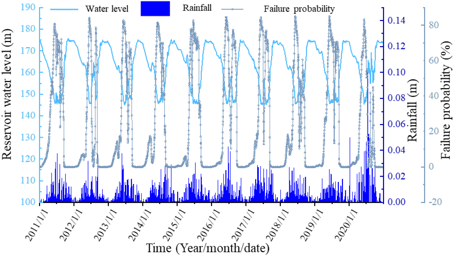
Variation in Pf during 2011–2020 for the Jiuxianping landslide.
Three evaluation indices, such as the determination coefficient (R2) defined in Equation 2, mean absolute error (MAE) defined in Equation 3, and root mean square error (RMSE) defined in Equation 4, are calculated for the deep learning models.
where N represents the total amount of the data; is the value of original data; is the predicted result; is the average of the original data.
4.3 Long-term failure probability
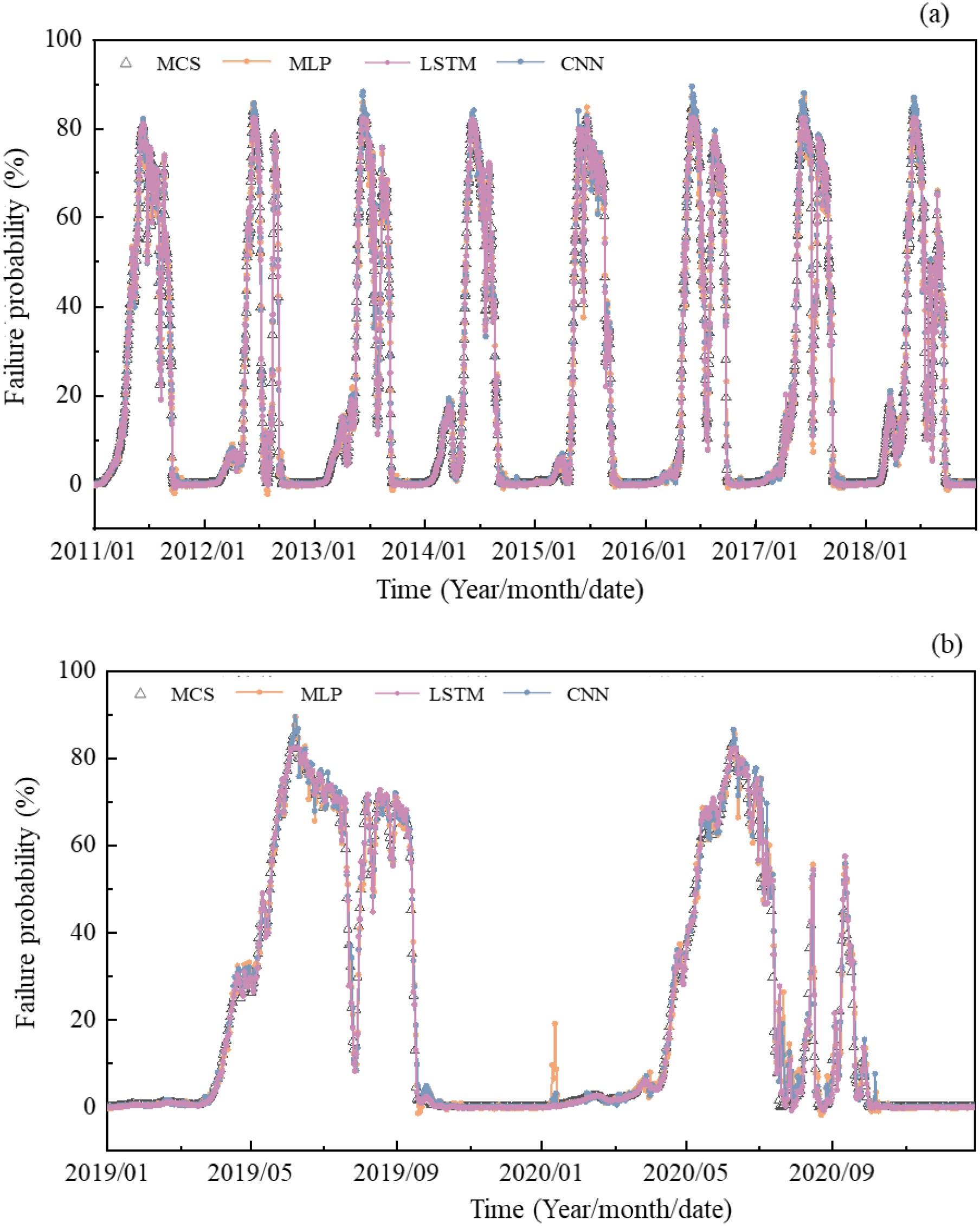
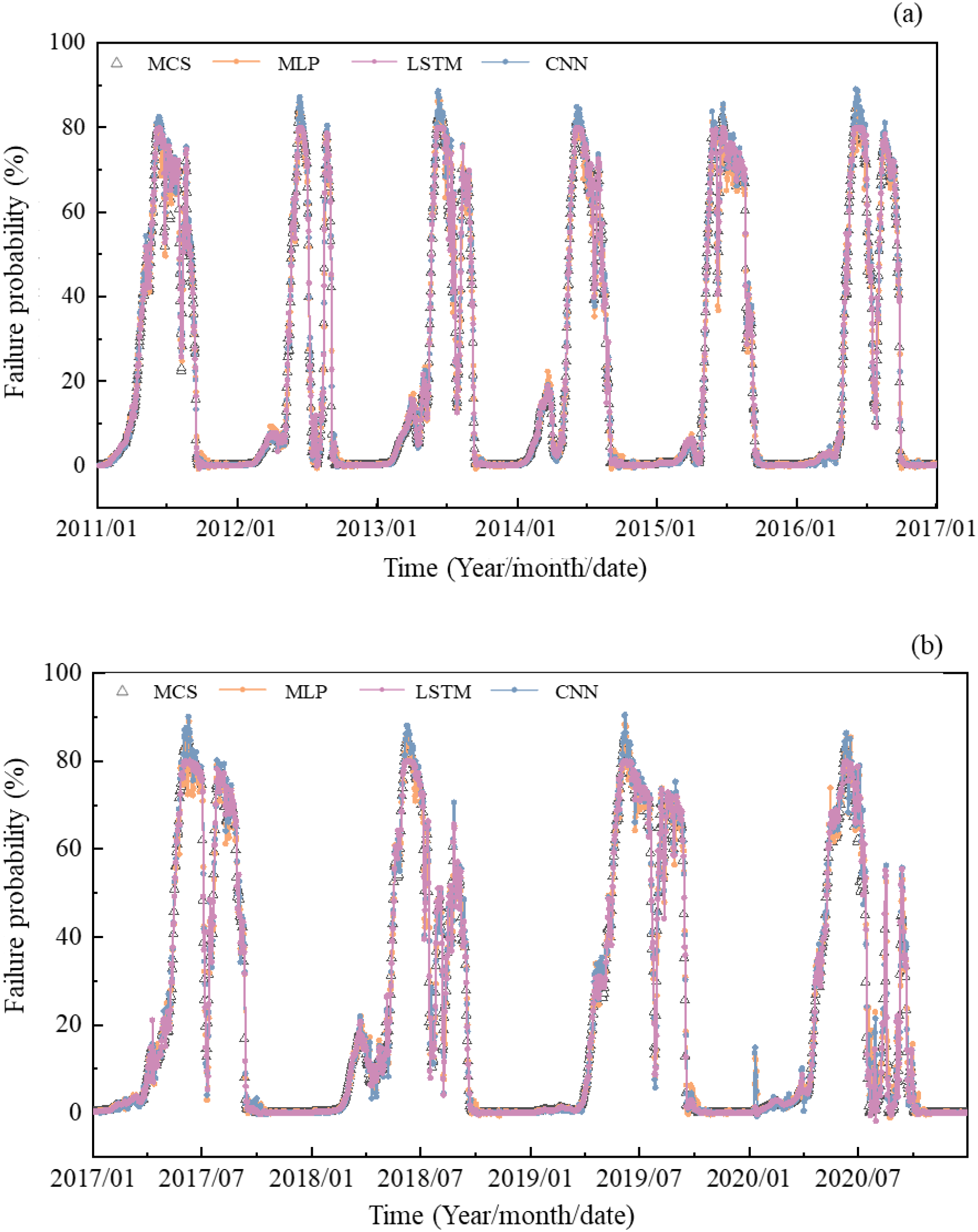
The structure of the MLP model consists of four fully connected layers. The structure of the CNN model consists of a total of three conv1D layers, which include a maxpooling1D layer and a global-average-pooling1D layer in the middle, and ends with a fully connected layer. In the LSTM model structure, four layers of LSTM are established, and the final layer is a fully connected layer. Figures 18, 19 shows the prediction results of three deep learning models compared with the training set and test set, respectively. Failure probability and its variation trend predicted by MLP, CNN, and LSTM models are generally consistent with the calculated value based on MCS in 2 figures. This indicates that time-series prediction based on deep learning models is of high accuracy. Moreover, these models are of high efficiency. While Slide 2 software takes about 35 minutes to compute the Jiuxianping landslide’s one-day failure probability, a deep learning model can predict decade-long Pf in just one minute. This drastically reduces computational demands for time-dependent reliability analysis and offers an effective solution for long-term landslide risk assessment. Other stability analysis methods for slope, such as the strength reduction method, are also applicable. This verifies the practical applicability of the novel method proposed in this study.
Figure 18
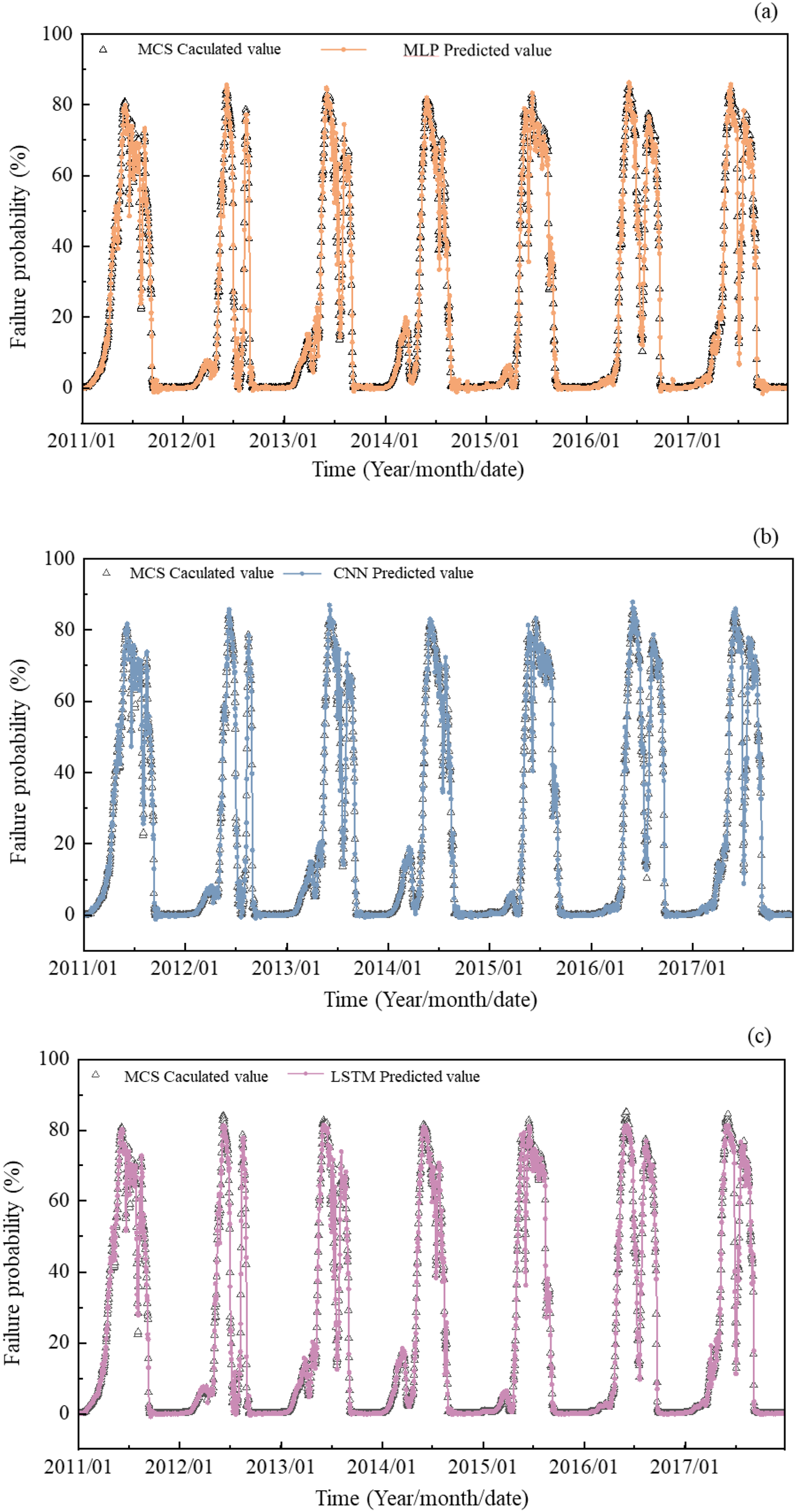
Failure probability predicted results compared with the training set using (A) MLP model, (B) CNN model, (C) LSTM model.
Figure 19
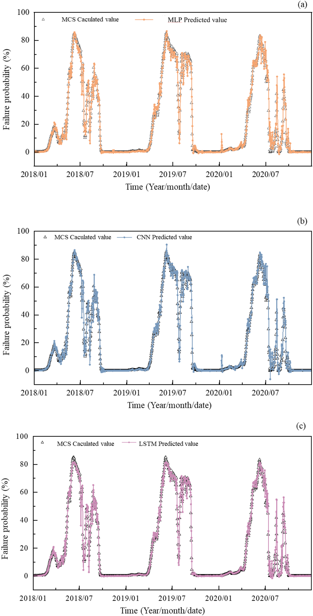
Failure probability predicted results compared with the test set using (A) MLP model, (B) CNN model, (C) LSTM model.
However, prediction results differ slightly when using different models. The MLP and CNN models may significantly overestimate or underestimate Pf when its corresponding calculated value is at the maximum or minimum. By contrast, the results predicted by the LSTM model deviate slightly from the extreme points, but the time-series curve predicted by the LSTM has smaller fluctuations, indicating the robustness of the LSTM model. The theoretical foundation of the MLP lies in its ability to approximate any continuous function through global, dense matrix operations. However, because it treats input features as an unordered set, the model lacks inherent awareness of temporal structure. As illustrated in the figure, while the MLP achieves reasonably accurate predictions overall, it struggles to reliably predict Pf at the next time step based on preceding parameter values—particularly at extreme points. In contrast, the CNN captures local features via convolutional filters. Its incorporation of pooling operations enhances robustness to minor local variations in the input, which explains why the CNN exhibits slightly better predictive performance in local regions compared to the MLP. The LSTM network, with its recurrent connections and gating mechanisms, is specifically designed to model temporal dependencies. As a result, it shows high adaptability and delivers precise predictions for tasks estimating failure probability in reservoir slopes with strong temporal correlations, where historical parameter values significantly influence future states.
Table 3 lists the calculated R2, MAE, and RMSE of 3 models. The R² values of all 3 models exceed 0.99 on the training set, indicating excellent goodness of fit. However, on the test set, R2 of the LSTM model is the highest (i.e., 0.9823), while R2 of CNN and MLP is 0.9784 and 0.9741, respectively. MAE represents the average absolute error, and is insensitive to outliers. Therefore, it has a stronger explanatory power for the regularity of time-dependent data. Among the three deep learning models, MAE value of LSTM is the smallest, followed by CNN. This indicates that these two models can overall predict the time-dependent characteristics the failure probability of bank slope. RMSE represents the overall error level, which amplifies larger errors and is highly sensitive to outliers. Among the three deep learning models, RMSE value of LSTM is still the smallest. This indicates that the LSTM model can better predict outliers, such as when the annual rainfall is particularly high and extreme situations may occur. In conclusion, it can be seen that the LSTM model performs well in predicting the long-term failure probability in this study.
5 Discussion
5.1 Total amount of data
This section discusses the performance of three deep learning method when data amount is changed. Firstly, the influence of the total amount of data on the prediction results is discussed. The structures of the three models remain unchanged. Meanwhile, in order to ensure the consistency of the changing trend of the predicted data, the data amount from 2011 to 2020 is reduced by half, that is, the data is from 2016 to 2020. The ratio stays the same. The data involving 2016–2019 and 2019–2020 are regarded as the training set and test set, with a data amount of 1274 and 546, respectively.
Figure 20 shows the prediction results when the data amount is reduced by half. It can be seen that the three models can still capture the changing trend of the time-dependent failure probability. Among them, the LSTM model still shows the best performance in estimating the failure probability value and varying trend. That is to say, the total amount of data has a limited effect on the time-series prediction.
Figure 20
Prediction results of three established DL models (A) training set; (B) test set.
Table 4 shows that reducing the input data amount does not degrade the prediction performance of any model. For example, as the MLP model generalization ability is relatively weak, its prediction may be greatly affected. However, the evaluation indices of the MLP model are not changed that greatly. R2 of the MLP model in the test set decreased from 0.9741 to 0.9579. MAE of the MLP model changed from 2.25 to 2.98, and the RMSE increased from 4.48 to 5.64. The error of the LSTM model is the smallest relative to alternative approaches, and it captures the time-dependent characteristic better. Therefore, the LSTM model is still superior to the others after reducing the data amount. It is reasonable to deduce that the 3 models can still predict the future failure probability of the Jiuxianping landslide accurately. This validates that the novel method can effectively predict long-term landslide failure probability even with limited input data.
Table 4
| Model | R2 | MAE | RMSE | |||
|---|---|---|---|---|---|---|
| Training set | Test set | Training set | Test set | Training set | Test set | |
| MLP | 0.9864 | 0.9579 | 1.86 | 2.98 | 3.46 | 5.64 |
| CNN | 0.9917 | 0.9690 | 1.49 | 2.59 | 2.7 | 4.84 |
| LSTM | 0.9931 | 0.9769 | 1.18 | 2.05 | 2.46 | 4.18 |
Evaluation index of three models for half amount input data.
5.2 Training and test set
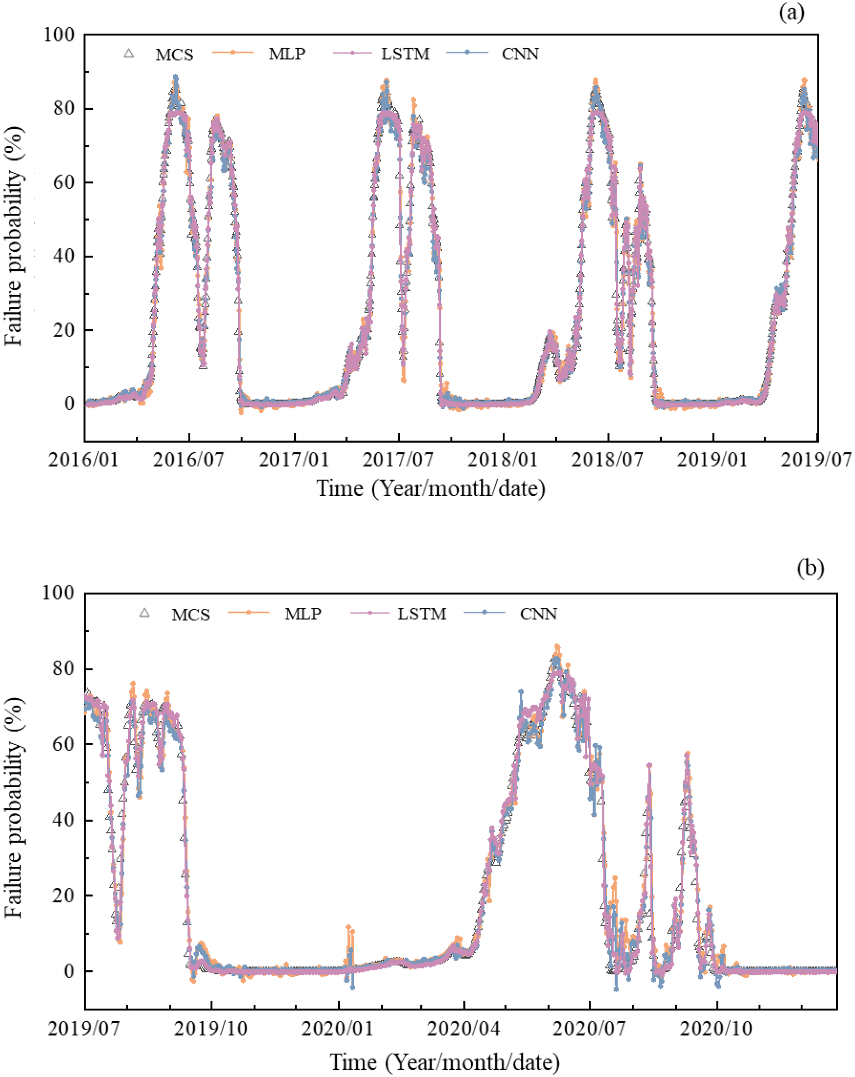
The ratio of the training set and the test set (named ratio hereafter for simplicity) is discussed in this section. The ratio is set as 8:2 and 6:4, respectively. Figures 21, 22 show the prediction results of the three models at a ratio of 8:2 and 6:4. It can be seen from the figures that the three models can still capture the changing trend of the time-dependent failure probability, as the prediction results are consistent with the calculated results. Compared with the CNN and MLP models, the failure probability predicted by LSTM rarely has sudden change points. It can be concluded that the prediction results of the LSTM model are relatively stable, showing strong robustness. It is verified that these models can still capture the changing trend of the time-dependent Pf when the ratio varies. However, there are still problems with accurately estimating the extreme points for all three models.
Figure 21
Prediction results of three models with a ratio of 8:2: (A) training set; (B) test set.
Figure 22
Prediction results of three models with a ratio of 6: (A) training set; (B) test set.
From the perspective of the evaluation indices as shown in the Table 5, the accuracy of the three models in capturing the variation of time-dependent failure probabilities has slightly decreased, but the overall prediction effect remains at a comparable level when the ratio is 7:3. For instance, compared with ratio of 7:3, in the test set, R2 of the LSTM model decreases to 0.9811 and 0.9823 respectively, with a reduction of only 0.0012 and 0.0009. The increase in MAE is only 0.04% and 0.08%, and RMSE increased by 0.21% and 0.26%. The fluctuation in the evaluation index is owing to the uncertainty of the training effect of deep learning every time. In short, the ratio changing from 7:3 to 8:2 or 6:4 does not improve the accuracy in capturing the time-dependent trend.
Table 5
| Ratio | Model | R2 | MAE | RMSE | |||
|---|---|---|---|---|---|---|---|
| Training set | Test set | Training set | Test set | Training set | Test set | ||
| 8:2 | MLP | 0.9898 | 0.9741 | 1.48 | 2.25 | 2.90 | 4.58 |
| CNN | 0.9924 | 0.9773 | 1.25 | 2.06 | 2.50 | 4.29 | |
| LSTM | 0.9921 | 0.9811 | 1.16 | 1.76 | 2.55 | 3.91 | |
| 6:4 | MLP | 0.9896 | 0.9754 | 1.51 | 2.22 | 2.94 | 4.46 |
| CNN | 0.9912 | 0.9765 | 1.41 | 2.18 | 2.71 | 4.35 | |
| LSTM | 0.9923 | 0.9806 | 1.13 | 1.84 | 2.54 | 3.96 | |
Evaluation indices of three models with a ratio of 8:2 and 6:4.
6 Conclusions
This study, aiming at the reservoir bank landslides under the influence of dynamic mechanical environment, takes the Jiuxianping landslide in the TGR as an example and proposes a novel prediction method for the long-term failure probability. This method, based on machine learning algorithms, can significantly reduce the calculation time when considering the spatial variability of rock and soil masses. Also, it can effectively depict the combined effect of reservoir water level and rainfall, and increase prediction accuracy at each time point the failure probability of reservoir bank landslides within ten years. The main conclusions drawn from the full text are as follows:
(1) Firstly, by analyzing the on-site geological and monitoring data, the failure mechanism of the Jiuxianping landslide and the time-dependent characteristics of displacement are obtained. The overall failure mechanism of the Jiuxianping landslide is sliding-bending mode, and the landslide goes through three stages: the slightly bended stage, the strongly bended and uplifted stage, and the slide surface formed stage Furthermore, significant deformation occurs during May to October each year, and the deformation positions are distributed in the middle and the leading edge, with almost the same displacement amounts, indicating that it is an overall slip. The displacement is not significant in other months, and the displacement develops as a stepped pattern. The deformation of landslides is mainly affected by the reservoir water level and rainfall. Compared with the influence of the water level decline, the influence of rainfall on the deformation of landslides is relatively small.
(2) The seepage field and safety factor of 2020 year is analyzed through the established landslide numerical model. The consistency of variation trend is found between the safety factor and reservoir water level. As the decline rate of the reservoir water level is greater than the permeability coefficient of the slope, it makes the infiltration line at the leading-edge of the landslide turn to an upward convex or upward concave shape when the water level increases or declines. Water level decline creates an outward hydrodynamic pressure, leading to the decrease in safety factor. That’s the main reason for safety factor decrease with water level of reservoir. On the contrary, water level increase makes the slope more stable. The upward convex or upward concave shape of the infiltration line is more obvious when the variation rate of water level is higher. Also, compared with rainfall, the safety factor is more sensitive to the reservoir water level.
(3) Reliability analysis is conducted on the Jiuxianping landslide in 2020 based on the random field model, considering spatial variability of cohesion and friction angle of the sliding zone. Results show that the failure probability increases with the decreasing of reservoir water level and this is consistency with the stability evaluation. Parametric study results show that the failure probability increase with any of the parameters such as COV, correlation coefficient of cohesion and friction angle or scale of fluctuation. However, among them, the effect of the correlation coefficient is the smallest. Moreover, the effect of COV of friction angle is bigger than that of cohesion.
(4) By calculating 10-year Pf using the random field model, this study proposes a novel method for predicting the long-term failure probability based on 3 deep learning models. 3 models can accurately describe the changing trend of the time-dependent failure probability of the Jiuxianping landslide, and can predict the future failure probability of the landslide. The calculation time decreases from 35 minutes of the daily failure probability to only 1 minute for ten years’ failure probability calculation. It has been proved that the novel method is effective. The prediction results of the LSTM model is superior to that of the other models. In the case of reducing the amount of the input data and changing the ratio of the training set to the test set, the three models can still reasonably predict the time-dependent failure probability. However, the prediction ability of the three models has not been improved.
This study also has some limitations. This study only considered the spatial variability of the shear strength of the sliding zone. In fact, some other property such as hydraulic parameters also shows spatially variable characteristic, and they vary with time under the dry-wet cycles. Therefore, the research results are applicable to the situations where the shear properties of the sliding zone are significantly different from sliding body. In future research, it is also possible to consider the spatial variability of multiple parameters throughout the entire landslide and to study the long-term dynamic changes considering properties change with time.
Statements
Data availability statement
The original contributions presented in the study are included in the article/supplementary material. Further inquiries can be directed to the corresponding author.
Author contributions
LW: Conceptualization, Data curation, Funding acquisition, Supervision, Writing – review & editing. TW: Investigation, Methodology, Software, Writing – review & editing. WY: Investigation, Methodology, Funding acquisition, Writing – original draft. YK: Data curation, Methodology, Validation, Writing – review & editing. XM: Conceptualization, Investigation, Methodology, Software, Writing – review & editing.
Funding
The author(s) declared financial support was received for this work and/or its publication. The current research is supported by the National Natural Science Foundation of China (52308340), China Postdoctoral Foundation (2024M753842), and the open fund of Chongqing Engineering Research Center of Automatic Monitoring for Geological Hazards (TICG-K2024002), the Postdoctoral Fellowship Program of CPSF under Grant Number GZC20242129, Open Research Fund of Key Laboratory of Geomechanics and Geotechnical Engineering Safety, Chinese Academy of Sciences (SKLGGES-024015).
Conflict of interest
The authors declare that the research was conducted in the absence of any commercial or financial relationships that could be construed as a potential conflict of interest.
Generative AI statement
The author(s) declare that no Generative AI was used in the creation of this manuscript.
Any alternative text (alt text) provided alongside figures in this article has been generated by Frontiers with the support of artificial intelligence and reasonable efforts have been made to ensure accuracy, including review by the authors wherever possible. If you identify any issues, please contact us.
Publisher’s note
All claims expressed in this article are solely those of the authors and do not necessarily represent those of their affiliated organizations, or those of the publisher, the editors and the reviewers. Any product that may be evaluated in this article, or claim that may be made by its manufacturer, is not guaranteed or endorsed by the publisher.
References
1
FanL. F.LehmannP.ZhengC. M.OrD. (2020). Rainfall intensity temporal patterns affect shallow landslide triggering and hazard evolution. Geophysical Res. Lett.47, 1–9. doi: 10.1029/2019GL085994
2
GuardianiC.SoranzoE.WuW. (2022). Time-dependent reliability analysis of unsaturated slopes under rapid drawdown with intelligent surrogate models. Acta Geotechnica17, 1071–1096. doi: 10.1007/s11440-021-01364-w
3
HuangM. L.SunD. A.WangC. H.KeletaY. (2021). Reliability analysis of unsaturated soil slope stability using spatial random field-based Bayesian method. Landslides18, 1177–1189. doi: 10.1007/s10346-020-01525-0
4
JiangS. H.HuangJ. S.GriffithsD. V.DengZ. P. (2022). Advances in reliability and risk analyses of slopes in spatially variable soils: A state-of-the-art review. Comput. Geotechnics141, 141. doi: 10.1016/j.compgeo.2021.104498
5
LiY.GuoZ.WangL.ZhuY.RuiS. (2024). Field implementation to resist coastal erosion of sandy slope by eco-friendly methods. Coast. Eng.189, 104489. doi: 10.1016/j.coastaleng.2024.104489
6
LiD. Q.JiangS. H.CaoZ. J.ZhouW.ZhouC. B.ZhangL. M. (2015). A multiple response-surface method for slope reliability analysis considering spatial variability of soil properties. Eng. Geology187, 60–72. doi: 10.1016/j.enggeo.2014.12.003
7
LiD.LiL.ChengY.HuJ.LuS.LiC.et al. (2022). Reservoir slope reliability analysis under water level drawdown considering spatial variability and degradation of soil properties. Comput. Geotechnics151, 104947, 1–12. doi: 10.1016/j.compgeo.2022.104947
8
LiL.LiC. L.WenJ. H.YuG. M.ChengY. M.XuL. (2023). Probabilistic seismic slope stability analysis using swarm response surfaces and rotational Newmark sliding model with primary sliding direction. Comput. Geotechnics163, 163. doi: 10.1016/j.compgeo.2023.105754
9
LiD. Q.WangL.CaoZ. J.QiX. H. (2019). Reliability analysis of unsaturated slope stability considering SWCC model selection and parameter uncertainties. Eng. Geology260, 105207, 1–13. doi: 10.1016/j.enggeo.2019.105207
10
LiY.WangL.DongC.FengG.SunX.GuoZ. (2025). A coupled mathematical model of microbial grouting reinforced seabed considering the response of wave-induced pore pressure and its application. Comput. Geotechnics184, 107235. doi: 10.1016/j.compgeo.2025.107235
11
LiD. Q.XiaoT.CaoZ. J.ZhouC. B.ZhangL. M. (2016). Enhancement of random finite element method in reliability analysis and risk assessment of soil slopes using Subset Simulation. Landslides13, 293–303. doi: 10.1007/s10346-015-0569-2
12
LiaoK.WuY. P.MiaoF. S.LiL. W.XueY. (2021). Time-dependent reliability analysis of Majiagou landslide based on weakening of hydro-fluctuation belt under wetting-drying cycles. Landslides18, 267–280. doi: 10.1007/s10346-020-01496-2
13
SuX. X.WuW.TangH. M.HuangL.XiaD.LuS. (2023). Physicochemical effect on soil in sliding zone of reservoir landslides. Eng. Geology324, 107249, 1–18. doi: 10.1016/j.enggeo.2023.107249
14
SunL. J.LiC. J.ShenF. M.ZhangH. Z. (2023). Reactivation mechanism and evolution characteristics of water softening-induced reservoir-reactivated landslides: a case study for the Three Gorges Reservoir Area, China. Bull. Eng. Geology Environ.82, 66, 1–23. doi: 10.1007/s10064-023-03084-9
15
Three Gorges Reservoir Area Geological Hazard Prevention Headquarters (2014). Technical requirements for engineering geological investigation of geological hazard prevention in Three Gorges Reservoir Area (Wuhan, Hubei Province: China University of Geosciences Press).
16
VagnonF.FerreroA. M.AlejanoL. R. (2020). Reliability-based design for debris flow barriers. Landslides17, 49–59. doi: 10.1007/s10346-019-01268-7
17
WangZ. Z.GohS. H. (2021). Novel approach to efficient slope reliability analysis in spatially variable soils. Eng. Geology281, 105989, 1–15. doi: 10.1016/j.enggeo.2020.105989
18
WangS.IdingerG.WuW. (2021). Centrifuge modelling of rainfall-induced slope failure in variably saturated soil. Acta Geotechnica16, 2899–2916. doi: 10.1007/s11440-021-01169-x
19
WangQ.OwensP. (2022). Reliability-based design optimisation of geotechnical systems using a decoupled approach based on adaptive metamodels. Georisk-Assessment Manage. Risk Engineered Syst. Geohazards16, 470–488. doi: 10.1080/17499518.2021.1884884
20
WuQ.LiuY.TangH.KangJ.WangL.LiC.et al. (2023). Experimental study of the influence of wetting and drying cycles on the strength of intact rock samples from a red stratum in the Three Gorges Reservoir area. Eng. Geology314, 107013, 1–23. doi: 10.1016/j.enggeo.2023.107013
21
WuY. P.MiaoF. S.LiL. W.XieY. H.ChangB. (2017). Time-dependent reliability analysis of Huangtupo Riverside No.2 Landslide in the Three Gorges Reservoir based on water-soil coupling. Eng. Geology226, 267–276. doi: 10.1016/j.enggeo.2017.06.016
22
XuJ. J.TangX. H.WangZ. Z.FengY. F.BianK. (2020). Investigating the softening of weak interlayers during landslides using nanoindentation experiments and simulations. Eng. Geology277, 105801, 1–12. doi: 10.1016/j.enggeo.2020.105801
23
YangY. J.LiD. Q.CaoZ. J.GaoG. H.PhoonK. K. (2021). Geotechnical reliability-based design using generalized subset simulation with a design response vector. Comput. Geotechnics139, 263–278. doi: 10.1016/j.compgeo.2021.104392
24
YangH. Q.ZhangL. L.PanQ. J.PhoonK. K.ShenZ. C. (2021). Bayesian estimation of spatially varying soil parameters with spatiotemporal monitoring data. Acta Geotechnica16, 263–278. doi: 10.1007/s11440-020-00991-z
25
YazdaniF.SadeghiH.AliPanahiP.GholamiM.LeungA. K. (2024). Evaluation of plant growth and spacing effects on bioengineered slopes subjected to rainfall. Biogeotechnics2, 100080. doi: 10.1016/j.bgtechs.2024.100080
26
YinY. P.HuangB. L.ChenX. T.LiuG. N.WangS. C. (2015). Numerical analysis on wave generated by the Qianjiangping landslide in Three Gorges Reservoir, China. Landslides12, 355–364. doi: 10.1007/s10346-015-0564-7
27
YuH. B.TangH. M.ZhouJ. Q.LiC. D.ZhangH. W.ZhuW. Y. (2023). An analytical model for assessing dynamic stability of bedding rock slope with soil interlayer under different rain patterns. Rock Mechanics Rock Eng. 57, 807–826. doi: 10.1007/s00603-023-03595-7
28
ZhangW. G.MengX. Y.WangL. Q.MengF. S. (2022). Stability analysis of the reservoir bank landslide with weak interlayer considering the influence of multiple factors. Geomatics Natural Hazards Risk13, 2911–2924. doi: 10.1080/19475705.2022.2149356
29
ZhangW. G.MengX. Y.WangL. Q.MengF. S.WangY. K.LiuP. F. (2023a). Reliability evaluation of reservoir bank slopes with weak interlayers considering spatial variability. Front. Mar. Sci.10, 10. doi: 10.3389/fmars.2023.1161366
30
ZhangW.TangL.LiH.WangL.ChengL.ZhouT.et al. (2020). Probabilistic stability analysis of Bazimen landslide with monitored rainfall data and water level fluctuations in Three Gorges Reservoir, China. Front. Struct. Civil Eng.14, 1247–1261. doi: 10.1007/s11709-020-0655-y
31
ZhangW. G.WuC. Z.TangL. B.GuX.WangL. (2023b). Efficient time-variant reliability analysis of Bazimen landslide in the Three Gorges Reservoir Area using XGBoost and LightGBM algorithms. Gondwana Res.123, 41–53. doi: 10.1016/j.gr.2022.10.004
32
ZhangP.XingG.HuX.LiuC.LiX.ZhaoJ.et al. (2024). Effects of grassland vegetation roots on soil infiltration rate in Xiazangtan super large scale landslide distribution area in the upper reaches of the Yellow River, China. Biogeotechnics2, 100104. doi: 10.1016/j.bgtech.2024.100104
33
ZhengG.WangJ.ZhouH.XiaB.BuiP. D. (2025a). Settlement characteristics and evaluation approach of embankment widening over soft clay. Can. Geotechnical J.62, 1–10. doi: 10.1139/cgj-2024-0413
34
ZhengG.ZhaoJ.YuX.ZhouH. (2025b). Calibration of partial factors for tensile strain design in geosynthetic-reinforced and pile-supported embankment. Transp Geotech.52, 101495. doi: 10.1016/j.trgeo.2025.101495
35
ZouZ.LuoT.ZhangS.DuanH.LiS.WangJ.et al. (2023). A novel method to evaluate the time-dependent stability of reservoir landslides: exemplified by Outang landslide in the Three Gorges Reservoir. Landslides20, 1731–1746. doi: 10.1007/s10346-023-02056-0
Summary
Keywords
bank slope, remote sensing, machine learning, spatial variability, long-term failure probability
Citation
Wang L, Wang T, Yang W, Kang Y and Meng X (2025) Machine learning-based improved method for estimating long-term failure probability with high efficiency of bank slope. Front. Mar. Sci. 12:1665294. doi: 10.3389/fmars.2025.1665294
Received
14 July 2025
Revised
12 September 2025
Accepted
17 November 2025
Published
17 December 2025
Volume
12 - 2025
Edited by
Qi Wang, Shandong Jianzhu University, China
Reviewed by
Liqin Zuo, Nanjing Hydraulic Research Institute, China
Liu Yang, Kunming University of Science and Technology, China
Updates
Copyright
© 2025 Wang, Wang, Yang, Kang and Meng.
This is an open-access article distributed under the terms of the Creative Commons Attribution License (CC BY). The use, distribution or reproduction in other forums is permitted, provided the original author(s) and the copyright owner(s) are credited and that the original publication in this journal is cited, in accordance with accepted academic practice. No use, distribution or reproduction is permitted which does not comply with these terms.
*Correspondence: Wenyu Yang, yangwy@cqu.edu.cn
Disclaimer
All claims expressed in this article are solely those of the authors and do not necessarily represent those of their affiliated organizations, or those of the publisher, the editors and the reviewers. Any product that may be evaluated in this article or claim that may be made by its manufacturer is not guaranteed or endorsed by the publisher.