Abstract
In the context of the rapid development of computer hardware and the continuous improvement of the artificial intelligence and deep learning theory, aiming at the traditional numerical solution method to solve the underwater acoustic fluctuation equation with large computational volume and the limitation of using various acoustic propagation models. We use the numerical solution calculated by the KRAKEN based on the normal mode theory, which is widely used in low-frequency shallow water waveguides, and combine it with the idea of solving the retarded envelope function in the parabolic equation theory. We propose a physical information neural network (PINN)-based method for intelligent prediction of the acoustic field using the elliptic fluctuation equation as the controlling equation. We conduct experiments under water body sound velocity varying stratified waveguide, to validate the model forecasting effect. It is experimentally verified that an effectively trained PINN network model can forecast the sound field at any given range. The predicted sound field can be used for a wide range of applications, such as sound source localisation and sonar range estimation.
1 Introduction
In the field of underwater acoustics, two methods are usually used to study the propagation of acoustic signals in seawater media. The first method is wave theory, which applies rigorous mathematical methods, combined with known fixed solution conditions, to solve the wave equation and study the change of amplitude and phase of acoustic signals in space. The second method is ray theory, in which the propagation of sound waves in a seawater medium is regarded as the propagation of sound lines in the medium in the high-frequency case; the change of sound intensity, the propagation time, and the propagation range of the sound lines in space are studied. Due to the approximation of ray theory, it is difficult to apply it in low-frequency shallow water conditions, and the importance of wave theory is particularly prominent in the context of the increasingly low frequency of sonar action. How to be able to solve the fluctuation equations accurately and quickly has become the focus of research by scholars in various countries.
As shown in Figure 1, under the assumption of linear acoustics, the basic control equation of underwater sound propagation, the wave equation (WE), can be obtained according to the equation of motion, continuity equation, and state equation. Due to the spatial and temporal complexity of the wave equation, it is difficult to solve it directly. Generally, the strategy adopted in practice is to convert the Fourier transform to the frequency domain to obtain the Helmholtz equation (HE) (Jensen et al., 2011).
Figure 1
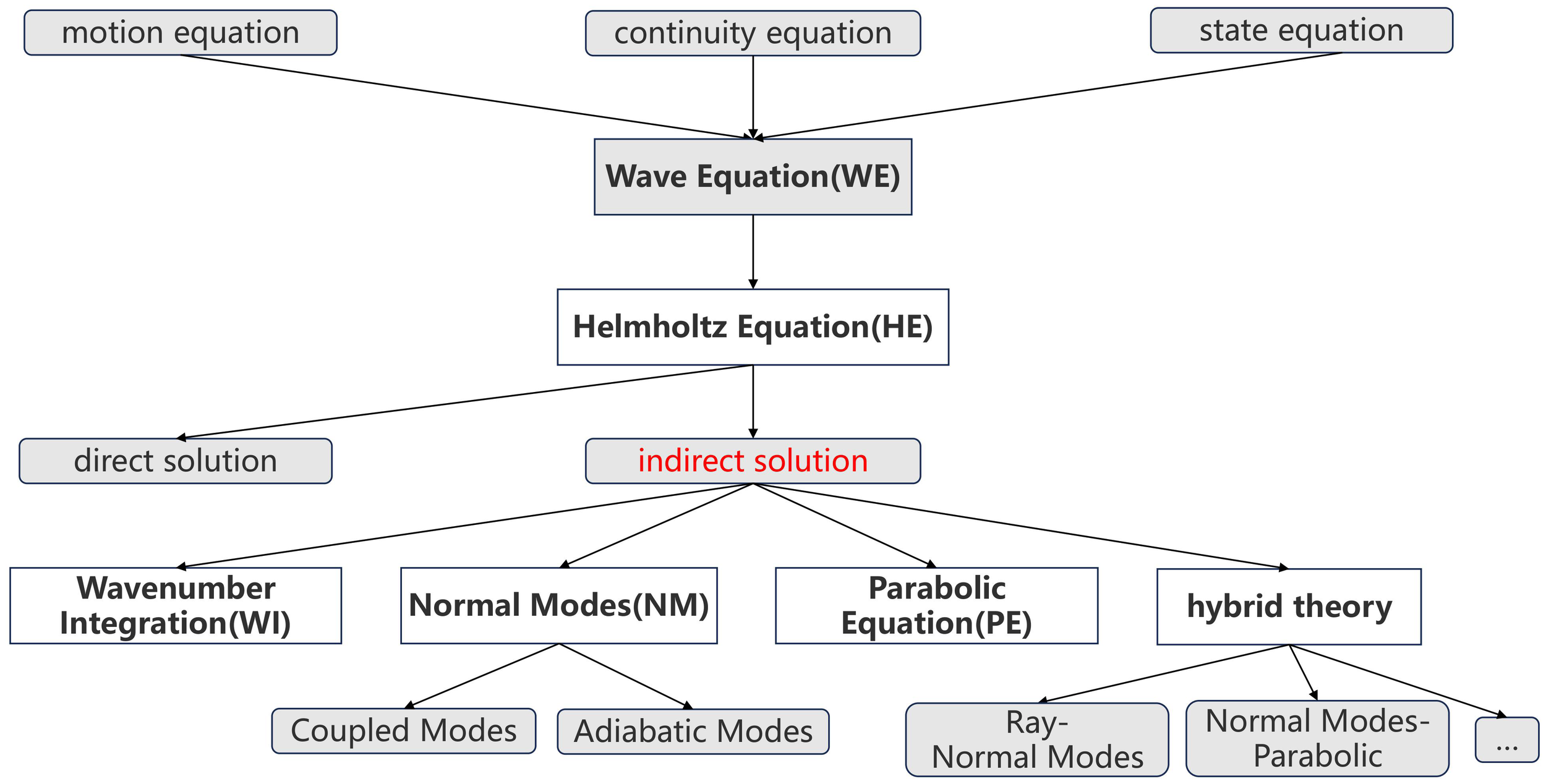
Methods for solving underwater acoustic wave theory.
Approaches to solving the Helmholtz equation are divided into two methods: direct and indirect. Solving the Helmholtz equation directly is difficult in practical applications, and the amount of computation is still staggering even today, despite the rapid development of computers. Liu et al. (2021) used the second-order and fourth-order difference formats to solve the Helmholtz equation directly for Lloyd’s mirror example with analytical solution, which took more than 1 hour and more than 1,000 iterations to reach convergence on a computer with 360 CPU cores, and the accuracy basically meets the requirements compared with the analytical solution, which is less usable in the actual sound field calculation.
Most of the solution ideas are solved by various simplified theories of Helmholtz equations; in the process of long-term exploration, simplified models based on the wavenumber integration (WI) theory (Schmidt and Glattetre, 1985), the normal mode (NM) theory (Godin, 1992), and the parabolic equation (PE) theory (Collis et al., 2008) are used. At present, most of the numerical solution methods are based on the development of the above theories or a combination of each other; these methods have their own advantages and disadvantages, and restrictions on the use of conditions, and there is no model that can be applied in any case.
Traditional numerical methods for solving partial differential equations (PDEs) are essentially solved discretely. For example, the finite difference method (FDM) (Stephen, 1988) solves partial differential equations by replacing differentiation with a difference approximation of the derivatives at grid points. The finite element method (FEM) (Thompson, 2006) solves the problem by dividing the solution domain into a finite number of small elements and then approximating the functional form of the solution on the elements. The finite volume method (FVM) (Fogarty and LeVeque, 1999) is based on the concept of control volume and divides the solution domain into multiple control volumes. The spectrum method (SM) (Tu et al., 2023) uses global basis functions (e.g., sine and cosine functions) to approximate the solution. Methods such as the boundary element method (BEM) (Lu et al., 2008) are widely used for solving PDEs, transforming the problem into integral equations on the boundary and discretizing only the boundary. These numerical discretization methods are currently widely used in underwater acoustic propagation model calculations and have an irreplaceable role for a short period of time.
With the continuous development of artificial intelligence (AI) and deep learning (DL), the application of AI is not only limited to traditional tasks such as computer vision, natural language processing, and speech recognition; the application of AI in various disciplines is more and more extensive, and the combination of AI and other disciplines has become one of the main research directions in this field. The combination of artificial intelligence and other disciplines has become one of the main research directions in this field. One of the applications of combining AI with mathematics, physics, and other disciplines is solving partial differential equations (Han et al., 2018).
In 1989, Cybenko (Cybenko, 1989) proved that a perceptron neural network with hidden layers has the ability to approximate any function when the activation function is a Sigmoid function, and in 1991, Hornik et al. (1989) further proved that the same applies when the activation function is any non-constant function. This is the fundamental theoretical basis of deep learning, universal approximation theorem (UAT), which describes the property that feedforward neural networks with a sufficient number of hidden units can approximate any continuous function to arbitrary accuracy, which is also known as the theoretical basis for neural networks to be able to solve PDEs.
With the rapid development of computer hardware technology and the arrival of the era of big data and deep learning, deep learning frameworks such as TensorFlow (Dean and Monga, 2015), PyTorch (Paszke, 2019), and PaddlePaddle (Ma et al., 2019) have been gradually generated, perfected, and developed, and AI is rapidly becoming a powerful tool for solving complex scientific problems. In particular, the application of AI is opening up new possibilities in the field of solving PDEs. The core of the emerging field of artificial intelligence for partial differential equations (AI4PDE) lies in the use of neural networks and other machine learning techniques to approximate the solution of PDEs, a method called a deep learning solver. Deep learning solvers are able to learn from data and automatically capture complex patterns and features of the problem to provide faster and more accurate solutions than traditional numerical methods.
Raissi et al. (2019) proposed physics-informed neural network (PINN), compared with the traditional purely data-driven neural network, by adding the difference between the physical equations before and after the iteration to the loss function of the neural network so that the physical equations are also “involved” in the training process, so that the neural network optimizes not only the network itself but also the difference between each iteration of the physical equations during the training iteration, and so that the final training result is to satisfy the physical laws at the same time. Compared with the traditional purely data-driven neural network, by adding the difference of the physical equations before and after the iteration to the loss function of the neural network, the physical equations are also “involved” in the training process so that the neural network optimizes not only its own loss function but also the difference of the physical equations in each iteration of the training iteration and so that the final training result is to satisfy the laws of physics and, at the same time, use fewer data samples to learn the model with a more generalization ability. This approach is known as the physics-driven approach, and PINN has been applied to quite a number of scientific and engineering problems, such as solving the Navier–Stokes equations, Schrödinger’s equations, and Maxwell’s system of equations. In addition, PINN can solve not only forward problems but also inverse problems. Among them, the forward problem mainly refers to the prediction of the sound field at different locations given the environmental information, and the inverse problem mainly refers to the inverse performance of the environmental information parameters from the information of the measured sound field data, and so on.
As shown in Figure 2, in contrast, there is also a class of methods that simply use labeled data for PDE solving, which are generally referred to as data-driven methods. This class of methods does not need to use the physical equations at all, but rather uses neural networks as operator approximators to solve parametric PDEs, using large amounts of labeled data to learn a direct mapping from the PDE parameters to the equation solutions. This includes Deep Operator Network (DeepONet) proposed by Lu et al. (2019) and Fourier Neural Operator (FNO) proposed by Li et al. (2020). However, in the actual complex underwater acoustic modeling process, the cost of obtaining valuable tagged data is often high, and the tagged data usually contain noise. Due to the main reliance on data-driven models, when the available labeled data are small or contain a lot of noise, the trained model has low accuracy and poor generalization ability, and at the same time, purely relying on data-driven models also lacks physical interpretability; thus, these methods have more limitations in practical applications and are currently only used for solving simpler PDE problems with a large amount of valuable labeled data. How to make full use of physical information to solve PDEs with high accuracy when there are little or no labeled data is a key issue to be solved.
Figure 2
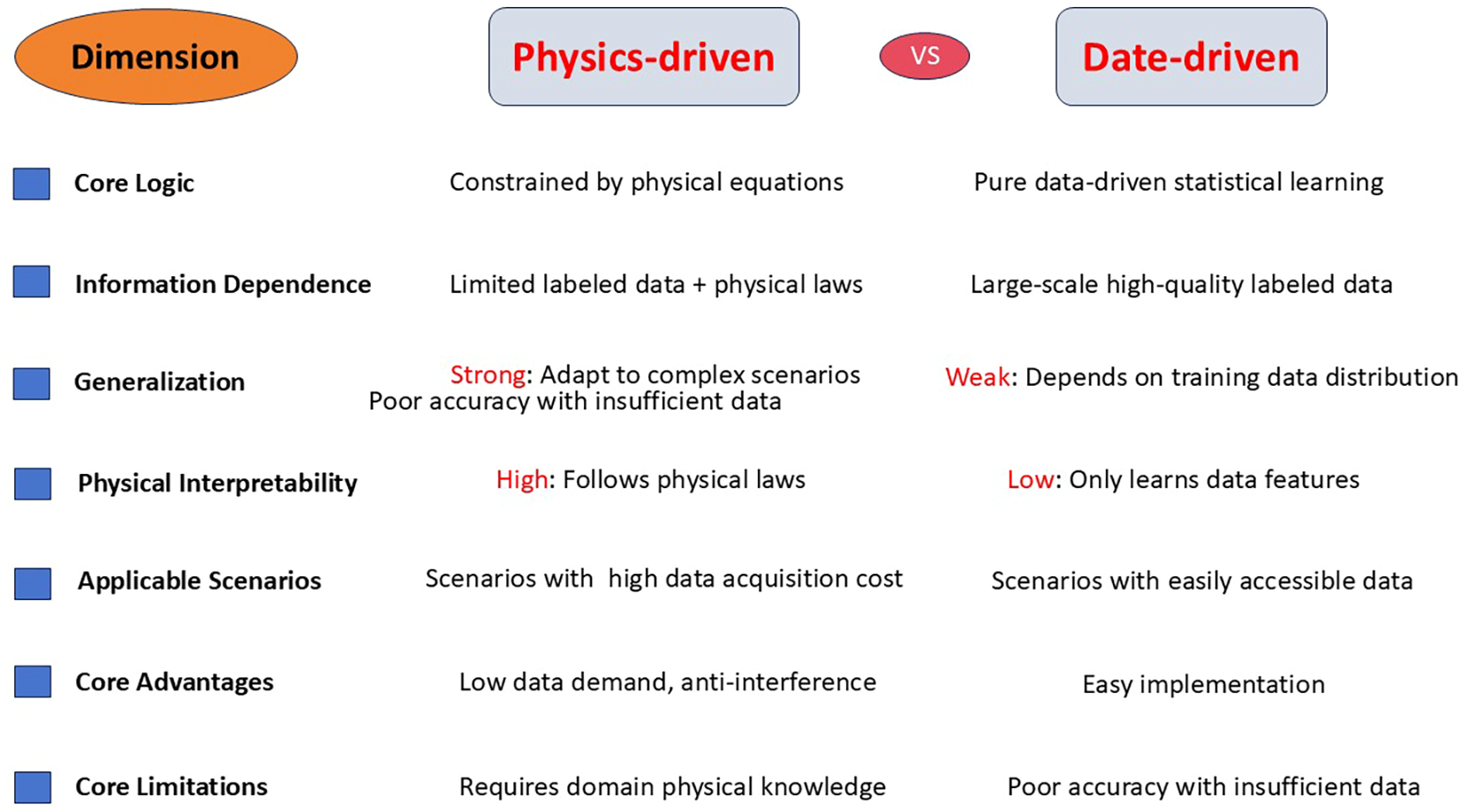
Physics-driven approach vs. data-driven approach.
In the course of previous research, there have been many scholars who have solved the underwater acoustic propagation problem by means of deep learning. Li and Chitre (2023) combined PINN with ray acoustics to propose a ray basis neural network (RBNN) and compared it with traditional data-driven machine learning methods—Gaussian process regression (GPR) and artificial neural network (ANN)—for reasonable extrapolation outside the data collection area through four numerical case studies and one ANN. GPR and ANN for reasonable extrapolation outside the data collection area, and the feasibility and applicability of the method are demonstrated through four numerical case studies and one controlled experiment. Du et al. (2023) proposed a physics-informed neural network (UAFP-PINN) using the COMSOL software to place a point source at the edge of the simulated two-dimensional (2D) and three-dimensional (3D) marine environment and to directly measure the acoustic field of a point source in the simulated 2D and 3D marine environment. A point source is placed at the edge of the simulated 2D and 3D ocean environment using the COMSOL software to directly solve the Helmholtz equation of the sound field, and the effectiveness of the method in forecasting the sound field is verified by comparison. Mallik et al. (2022) proposed a convolutional recurrent autoencoder network (CRAN) structure, which is a data-driven deep learning model for directly learning acoustic transmission loss in the far field. It is also proposed that the generalization ability of CRAN can be effectively improved by double-checking the errors in the validation set, appropriate hyperparameter tuning, and stopping the training of CRAN earlier. Duan et al. (2024) proposed a spatial domain decomposition-based physics-informed neural network (SPINN). By generating a range-independent sound field for the RAM model, by adding noise, and by inputting a noise-containing dataset for experiments, they quantitatively analyzed the effects of three influencing factors, namely, sound speed error, marine environmental noise, and observation noise, on the ability of SPINN to learn the sound field by means of root mean square error (RMSE), and compared it with the PINN without spatial domain decomposition. Comparison with PINN without spatial domain decomposition demonstrates the good performance of SPINN. Gao et al. (2024) proposed a fast computational method for underwater acoustic field based on PINNs, in which the frequency-domain Helmholtz equations, which represent the underwater acoustic propagation law, are encoded as physical neurons through automatic differentiation and combined with a small amount of measurement data as informative neurons to construct a physically informative and data-driven neural network to solve the underwater acoustic field. Huang et al. (2024) proposed a fast computational method for underwater acoustic field based on PINNs, in which the frequency-domain Helmholtz equations, which represent the underwater acoustic propagation law, are encoded as physical neurons through automatic differentiation and combined with a small amount of measurement data as informative neurons to construct a physically informative and data-driven neural network to solve the underwater acoustic field. Huang et al. (2024) proposed a fast broadband modeling method using a physics-informed neural network by integrating the modal equations of normal modes as a regular term in the loss function of the neural network, which enables fast broadband modeling of the underwater acoustic channel in the presence of sparse frequency sampling points.
In terms of the research content, the current research mainly shows the combination of numerical solution methods or deep learning solution methods with classical underwater acoustic propagation theory; the solution method and theory each belong to a dimension, and the combination of a solution method and a theory can produce a new underwater acoustic propagation model. As shown in Figure 3, the research content of this paper mainly focuses on the combination of PINN with the theory of normal modes and the theory of parabolic equations.
Figure 3
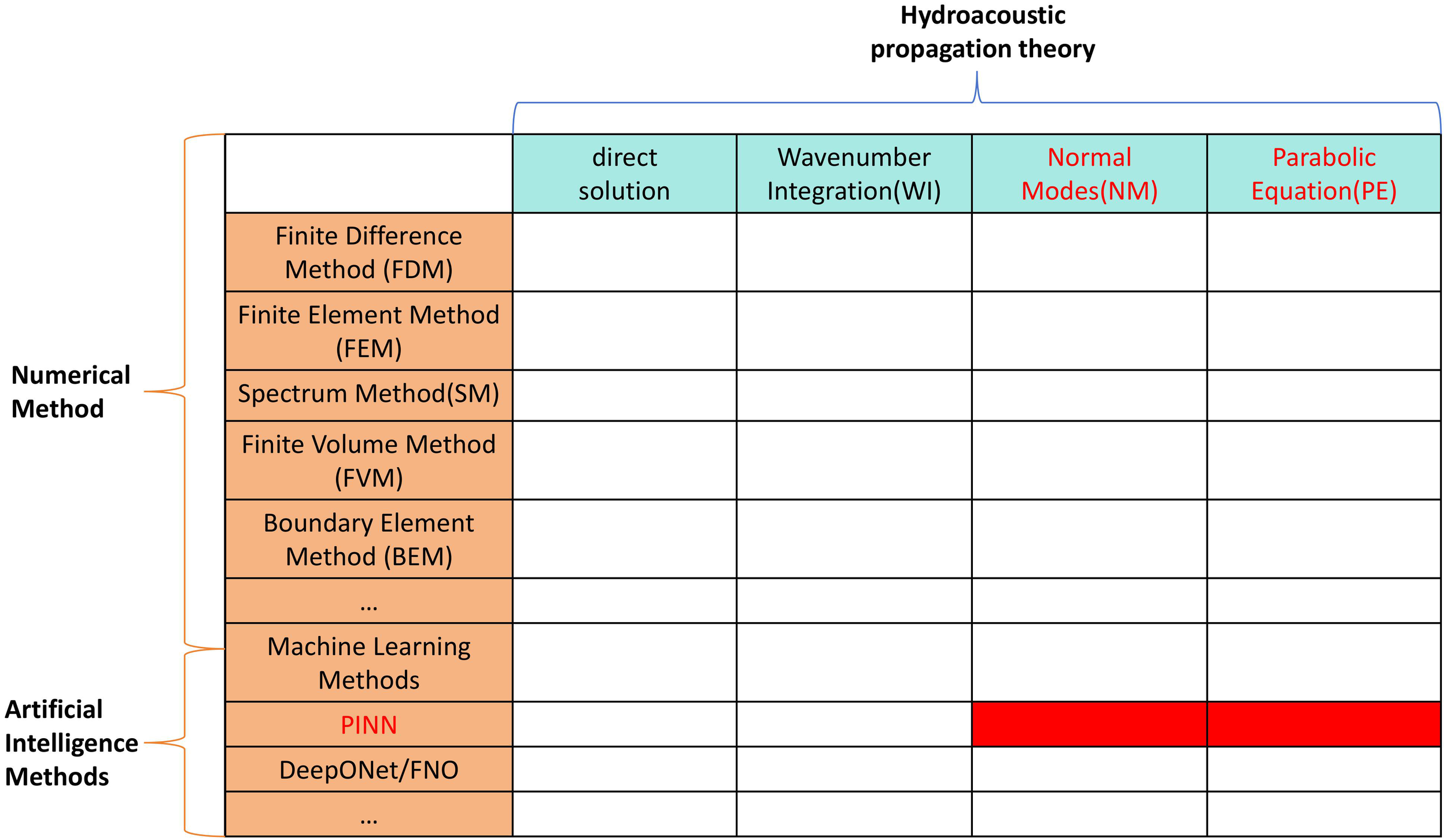
Highlights of the research content of this paper (red areas).
2 PINN model structure and theory
As summarized in the preceding analysis, the current field of underwater acoustic field prediction faces three core challenges: traditional numerical methods (e.g., finite difference method and KRAKEN software based on NM theory) suffer from large computational volumes and poor adaptability to complex stratified waveguides; pure data-driven models (e.g., DeepONet) rely on massive labeled data, which are costly to acquire and noisy in real marine environments, leading to weak generalization; and existing PINNs mostly integrate only a single physical equation (e.g., Helmholtz equation), failing to leverage the multi-scale physical characteristics of underwater acoustic propagation and resulting in suboptimal accuracy in complex scenarios. To address these issues, this study proposes a systematic innovation centered on a dual-physics-constrained PINN framework, which fuses NM theory and PE theory.
The specific innovations are as follows: theoretically, NM theory is used to generate physically meaningful prior data (modal functions and horizontal wavenumbers of each order) via the KRAKEN software, avoiding the “modal aliasing” problem of existing PINNs caused by random prior data; PE theory converts rapidly fluctuating sound pressure signals into slowly varying envelope functions, reducing the difficulty of neural network learning and solving the convergence issue of direct sound pressure training; meanwhile, the elliptic fluctuation equation derived from PE theory is adopted as the control equation of PINN, which not only retains the computational advantages of parabolic approximation but also inherits the modal information of NM theory, avoiding the approximation errors or computational complexity of existing control equations (e.g., Helmholtz equation). Methodologically, the PINN loss function design is optimized: the total loss includes three components (data-driven term for fitting NM-derived envelope data, boundary constraint term for applying sea surface pressure release conditions, and physical constraint term for minimizing the residual of the elliptic fluctuation equation); considering that the physical constraint term is usually two orders of magnitude smaller than the other two terms, its weight is adjusted to prevent it from being “overwhelmed”, balancing data fitting and physical consistency, which is different from the equal-weight design of existing PINNs. Practically, the framework integrates seabed parameters through NM theory to adapt to stratified waveguide environments and relies on the physical prior information provided by NM and PE theories to reduce the demand for labeled data, enabling high-precision prediction without massive samples and lowering the cost of real-world deployment. This innovation not only addresses the aforementioned three challenges but also provides a more efficient and accurate technical path for practical applications such as sound source localization and sonar range estimation.
In the course of our research, we propose a deep learning approach to use PINN for forecasting the underwater sound field. While integrating the a priori information, PINN is fitted to a portion of the actual computed data. PINN utilizes envelope amplitude data at different depths for data fitting, which is its data-driven part. In addition to fitting the data at the sampling points, the PINN incorporates physical drivers, including the standard parabolic equations governing the PDEs themselves and the surface pressure release boundary conditions, to extend the sound field prediction to unknown points. The network requires a sound speed profile (SSP) and ocean substrate information (including density ρ, sound speed c, and attenuation coefficient α) as a priori information, and KRAKEN is used to compute the actual sound pressure data at the sampling points. According to the conclusion drawn by Du et al. (2023) in training the network, it can be seen that it is difficult to train the neural network directly using sound pressure data to converge to an exact solution due to the rapidly fluctuating nature of sound pressure data in a wide ocean environment with a range of kilometers, so we convert the rapidly varying sound pressure into a slow-varying envelope function and adding it to the neural network for training. After training, the PINN can predict the sound field at any . The predicted sound field is used in a wide range of applications, such as sound source localization and sonar action range estimation.
In the following, we will briefly introduce the principle of calculating sound pressure by normal modes in Section 2.1. Section 2.2 illustrates the conversion relationship between sound pressure and envelope function and introduces the elliptic fluctuation equations. Section 2.3 explains the network design idea of PINN and the basic principle of how to sample and get the envelope function by training.
2.1 Calculation of sound pressure by normal mode theory
The normal mode theory was first proposed by Pekeris in 1948 (Pekeris, 1948) to solve the acoustic propagation problem in a range-independent environment, and nowadays, it is one of the classical theories for solving acoustic propagation problems in shallow water. With the development of computer technology, Porter (1992) developed the KRAKEN software based on the finite difference method, which has the advantages of computational stability, accuracy, and speed, and this model is one of the widely used numerical computation programs for normal modes in underwater acoustics.
A brief introduction to the normal mode theory for solving the sound field is given according to Section 5.2 of Computational Ocean Acoustics (Second Edition) (Jensen et al., 2011), and we start with the 2D Helmholtz equation, where the sound velocity and density depend only on the depth z:
Use the technique of variable separation:
Substituting Equation 2 into Equation 1 and separating the constant yields
This is the most important equation in the theory of normal modes—in the modal equation, is the th order mode, where is the horizontal wavenumber, is the mode function, and the above equation is the classical Sturm–Liouville eigenvalue problem, where the goal is to find its eigenfunctions and eigenvalues .
The sound pressure can be obtained by synthesizing the sound field through Equation 4 by simply requiring the modal function in Equation 3 with the horizontal wavenumber.
We use KRAKEN to calculate the modal functions and horizontal wavenumbers corresponding to each order of modes from the given SSP and environmental information such as ocean substrate information (including density ρ, sound speed c, and attenuation coefficient α), as well as reasonable settings of various parameters that may affect the number of modes m in the environment (env) file and the field (flp) file, such as the frequency f, the minimum phase velocity , and the maximum phase velocity . The modal function and horizontal wavenumber corresponding to each order mode are calculated, and the sound pressure is obtained through Equation 4, which is used as the input quantity in Section 2.2.
2.2 Introduction of elliptic fluctuation equations
According to Section 6.2 of Computational Ocean Acoustics (Second Edition) (Jensen et al., 2011), the standard 2D Helmholtz equation in the column coordinate system is
where is the sound pressure, is the reference wavenumber, and is the refractive index.
Take the solution of Equation 5 in the following form:
where the envelope function is slowly varying with range and satisfies the following Bessel differential equation:
Substituting Equation 6 into Equation 5 and using the property of in Equation 7 gives
Next, we take the far-field approximation at which point can be replaced by its asymptotic form:
The simplified elliptic fluctuation equation can be obtained by bringing Equation 9 into Equation 8:
The Equation 10 is the most important control equation in the PINN we designed and is also different from the direct use of Equation 11
as the control equation (Du et al., 2023; Duan et al., 2024) in previous studies.
The sea surface pressure release boundary uses the first type of boundary conditions, also known as the Dirichlet boundary condition (DBC) as shown in Equation 12:
2.3 Network design for PINN
The biggest difference between PINN’s ability to accurately solve PDEs and numerical methods is the application of the neural network’s automatic differentiation (AD) technique. Unlike traditional analytic differentiation or numerical differentiation methods, automatic differentiation is able to automatically compute derivatives with arbitrary accuracy, which has a significant advantage, especially for complex function derivation. Automatic differentiation is used in deep learning to compute the gradient of the loss function with respect to the network parameters for parameter updating and optimization.
As shown in Figure 4, the structure of the PINN we designed mainly consists of an input layer, L hidden layers, and an output layer, with a total of layers, where layer 0 is the input layer, layers 1 to L are the hidden layers, and layer is the output layer. The number of neurons in the input layer is 2, which are range r and depth z. The L hidden layers are fully connected layers, where the number of neurons in the kth layer is . Since the envelope function is complex, the neural network cannot be trained directly on the complex numbers, so it needs to be split into the real part and the imaginary part and then trained; then, the number of neurons in the output layer is 2, which are and .
Figure 4
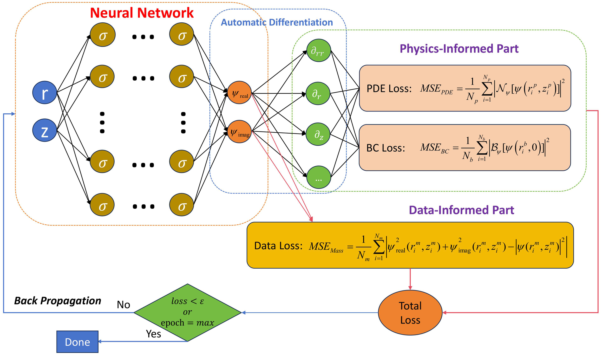
The PINN structure designed in this paper. PINN, physics-informed neural network.
According to the conclusion of Song et al. (2022) for PINN solving Helmholtz equation, it can be seen that the use of adaptive sinusoidal activation function Sine can be a good solution to the frequency-domain wavefield problem, so we use as the activation function; then, the computational structure of feedforward neural network as shown in Equation 13
where and denote the weights and biases, respectively, from the lth layer to the th layer.
For simple, physically meaningful PDE problems without the time term t, PINN can be trained by sampling only the interior and boundary points, under the control of PDEs and boundary conditions (BCs), allowing the network to learn the physical processes and extrapolate them for prediction. However, for the complex ocean acoustic propagation problem, it is difficult to use only the PDE loss term and BC loss term in the original PINN structure for purely physical driving to be effective, and in order to improve the accuracy of our prediction, it is necessary to use a part of the exact solution as the labeled data to incorporate the loss term as the data-driven part. Therefore, our loss function term consists of three parts as shown in Equation 14.
where each loss function is calculated using mean squared error (MSE) as shown in Equations 15–17, with being the loss of the data-driven term, being the loss of the BC control term, and being the loss of the PDE control term. The weights of each item are , , and .
where is the number of sampling points of the exact solution data, and is the set of coordinate values of its input network. is the number of equally spaced sampling points at the soft boundary of the sea surface, and is the set of coordinate values of its input network. is the number of random sampling points inside the computational domain, and is the set of coordinate values of its input network. and denote the differential operators for the boundary and inside the computational domain for the envelope function , respectively, and the specifics can be expressed by Equations 18–20:
When is less than the critical condition value set in advance or when the number of training rounds Epoch reaches the maximum value set in advance, the training is stopped, and the model parameters are saved; otherwise, backpropagation (BP) is continued, and the model parameters are updated.
When using the trained model for sound field prediction, the parameters of the model are loaded, and the range of the test set is set reasonably; the real and imaginary parts and respectively, of the envelope function of the test set in range are obtained by model prediction and synthesized to obtain the envelope function, which is then converted to obtain the sound pressure by Equation 21 and plotted by Equation 22 for the one-dimensional (1D) and 2D transmission loss (TL) to validate the accuracy of the method and the effectiveness of the prediction. TL is compared with the numerical solutions calculated by KRAKEN to verify the accuracy of the method and the validity of the forecast.
3 Research content and analysis
3.1 Isovelocity waveguide with constant velocity of sound in the water column
For the water body sound velocity invariant isovelocity waveguide, we take a kind of Pekeris shallow sea waveguide environment with sedimentary layer added as an example and set the water depth as 100 m, the seafloor as an acoustic semi-infinite space covered with a layer of 20-m-thick sedimentary layer, the sound velocity profile as isoacoustic velocity invariant, the depth of the source as 25 m, and the frequency as 100 Hz. Specific environment parameter information is shown in Figure 5.
Figure 5
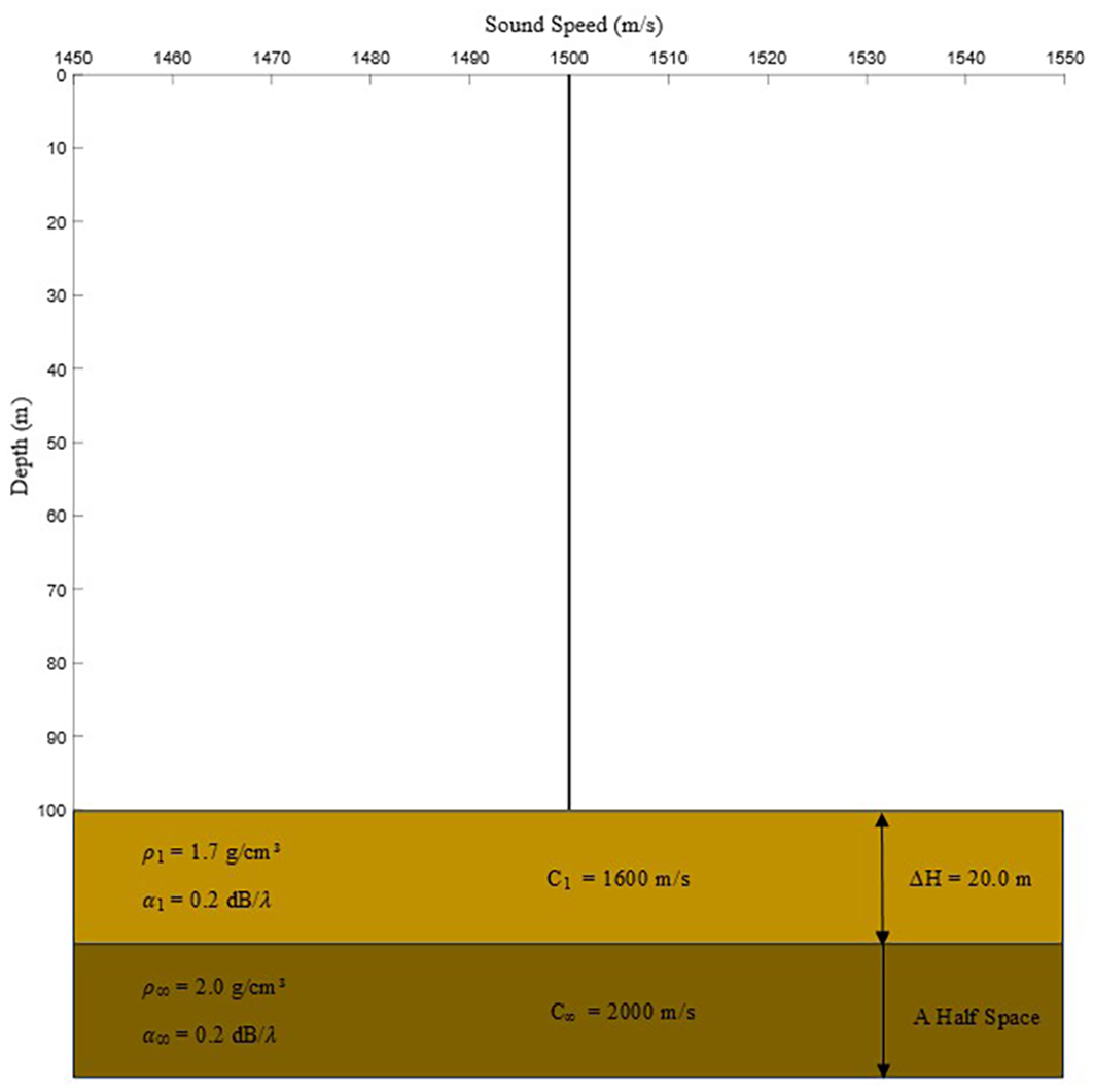
Environmental parameters of the Pekeris shallow water waveguide added to the sediment layer.
The specific parameters are shown in Table 1. The receiver depth range is determined based on the acoustic stratification characteristics of shallow-sea water, avoiding interference from bubble scattering near the sea surface (z < 10 m) and strong absorption by sediments at the seabed (z > 90 m). Meanwhile, three key depths (25, 50, and 75 m) are selected: 25 m is in the surface layer, slightly affected by sea surface reflection; 50 m is in the middle layer, where propagation is stable with little modal interference; 75 m is in the bottom layer, slightly affected by reflection from seabed sediments. These depths are used to comprehensively verify the model’s performance in different propagation environments.
Table 1
| Parameter category | Parameter name | Value |
|---|---|---|
| Source parameters | Source depth | 25 m |
| Source frequency | 100 Hz | |
| Receiver parameters | Receiver depth range | 10–90 m |
| Key receiver depths | 25, 50, 75 m | |
| Spatial range | Propagation distance range | 1,000–9,000 m |
| Environmental parameters | Seabed sediment thickness | 20 m |
Experimental parameter description table.
Firstly, using the KRAKEN software, the environment (env) file is set reasonably, and the phase velocity range is set to 0–5,000 m/s. A total of 15-order modes are excited for the synthesis of the sound field, and the horizontal wavenumbers and mode functions are shown in Figures 6a–c.
Figure 6
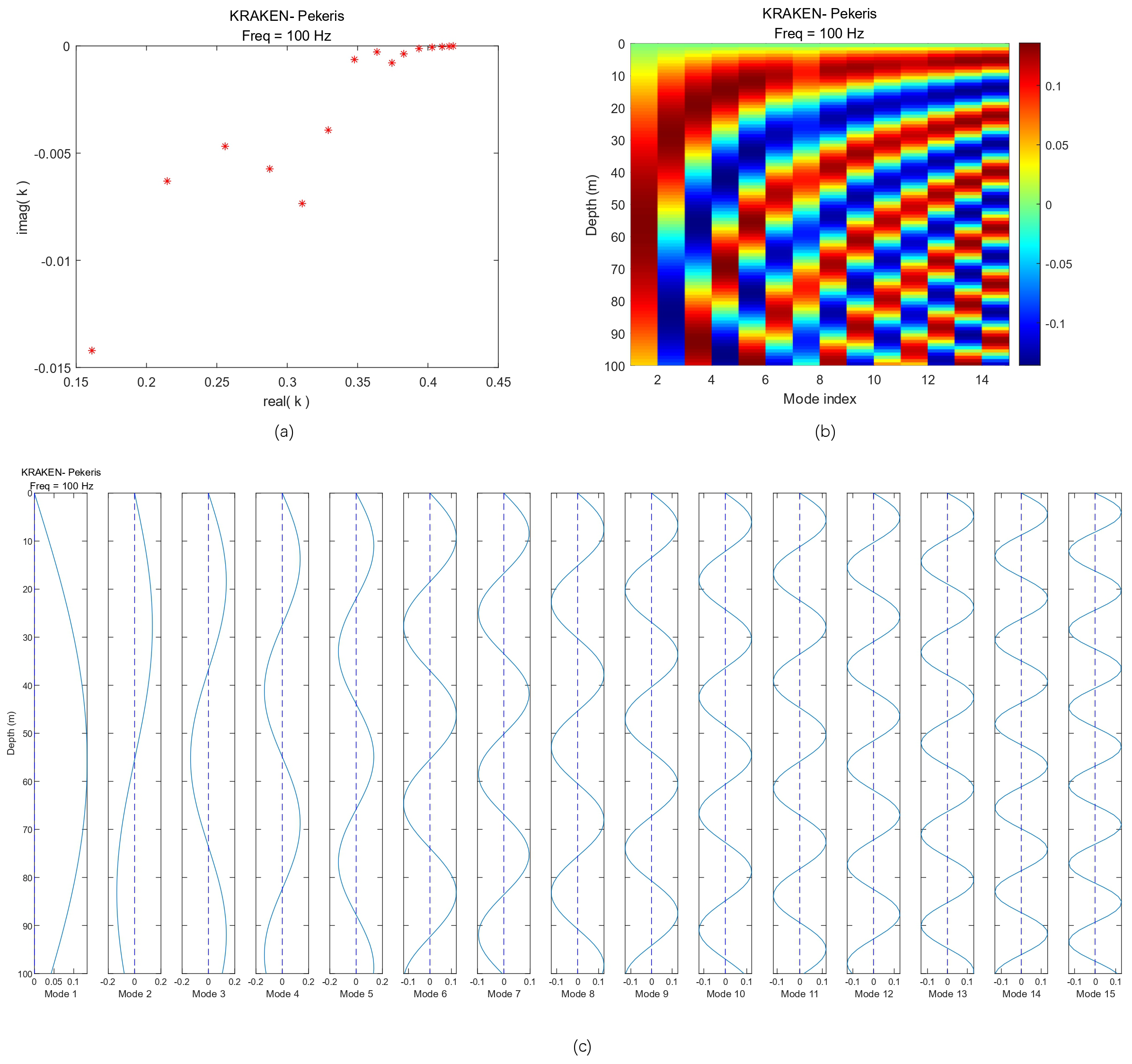
Pekeris waveguide for synthesis of sound field with horizontal wavenumber and modal function . (a) Scatterplot of real and imaginary parts of horizontal wavenumber . (b) Pseudo-color map of modal function (real part). (c) Plot of the real and imaginary parts of the modal function .
Since Equation 8 adopts the far-field approximation and combines with the actual sound field forecasting application requirements, a part of the receiving points are set to calculate the exact solution as the labeled data to be used for data driving. By setting the field (flp) file, set the receiving area r range of 2,000–8,000 m, every interval of 10 m to take a point, a total number of points = 601. Z range is 10–90 m, every interval of 10 m to take a point, with a total number of points = 9. The total number of sampling points nr * nz of the exact solution data is 5,409. The generated sound pressure is transformed into an envelope function through Equation 23; the total number of sampling points is 5,409. The generated sound pressure data are transformed into the envelope function :
This equation is obtained by reasoning from Equation 6. The envelope function is then split into real part and imaginary part to be used as input for the training set of the neural network.
According to the description of PINN training in Section 2.3, the sampling area inside the computational domain is set in the range of 1,000–9,000 m for r and 0.1–100 m for z. Considering the complexity of the problem, the GPU memory size limitation, the length of the training model, and the accuracy requirement, the number of random sampling points inside the computational domain is set to be = 5,000. The sampling area r was set to range from 1,000 to 9,000 m at the soft boundary of the sea surface, z was set to 0 m, and the number of equally spaced sampling points was set to = 200.
According to the findings of Du et al. (2023), it can be seen that the weight settings of the three loss function sources have a significant impact on whether the model training is successful or not, and we are guided by their findings to set the weights of the loss function as .
The experimental training is run on Aurora supercomputing server nodes with four NVIDIA Tesla V100 32GB graphics cards. The deep learning framework and version used is TensorFlow 2.5, and the optimizer used is Adam with a learning rate of 0.001. The number of hidden layers, L = 5, is used with a fully connected layer, and the number of neurons in each layer, = 100.
During the test, the random sampling area r is set to range from 1,000 to 9,000 m, and z is set to range from 0 to 100 m. By setting the field (flp) file in advance, the results calculated by KRAKEN in the same area are obtained for comparison to verify the accuracy of the method and the effectiveness of the prediction.
When the number of training rounds is 12,000, the model is saved, and a forecast is made, as shown in Figure 7, plotting the PINN forecast against the KRAKEN numerically calculated 2D transmission loss.
Figure 7
Epoch = 12,000, λMass:λBC:λPDE = 1:1:1, PINN vs. KRAKEN 2D transmission loss pseudo-color maps with errors. (a) PINN forecast result. (b) KRAKEN calculation result. (c) Error between the two results. PINN, physics-informed neural network.
It can be concluded that regions with a small number of accurate solutions, as labeled data, are forecasted with higher accuracy, and most of the regional forecasts are basically comparable to the accuracy of the KRAKEN numerical solutions with an error of 0 dB (Figure 7c, red part). In contrast, simply relying only on purely physical drive, in the internal and boundary random sampling point region, can only roughly reflect the trend of the transmission loss; the accuracy of the error is larger, and it is only suitable for use when the accuracy requirements are not high. It also quantitatively proves the reasonableness of the design of the network structure of this paper in Section 2.3. Relying solely on the physical process for extrapolation is less effective, while the accuracy of the forecast results is significantly improved after adding the data-driven process, which shows the importance of relying on high-quality labeled data for the data-driven deep learning of the complex ocean dynamics process.
Setting the reception depth to 25, 50, and 75 m plots the PINN prediction against the 1D transmission loss calculated from KRAKEN values, as shown in Figure 8.
Figure 8
Epoch = 12,000, λMass:λBC:λPDE = 1:1:1, PINN vs. KRAKEN 1D transmission loss. (a) Comparison of 1D transmission loss at a reception depth of 25 m. (b) Comparison of 1D transmission loss at a reception depth of 50 m. (c) Comparison of 1D transmission loss at a reception depth of 75 m. PINN, physics-informed neural network.
According to the results, it can be seen that PINN has poor learning ability for some extreme points, but good learning ability for some slow-change regions. Since the transmission loss curve at 50 m is smoother than that at 25 and 75 m, and the variation is smaller, PINN learns well, and basically agrees with the results of KRAKEN’s calculation in the range of 2,000–8,000 m except for some extreme points.
Based on the results, we believe that the poor results may be due to model underfitting, so we grow the number of training rounds to 50,000, with other conditions remaining unchanged, and again compare the 1D and 2D transmission loss.
At this point, the model is saved, and a forecast is made, as shown in Figure 9, plotting the PINN forecast against the KRAKEN numerically calculated 2D transmission loss.
Figure 9
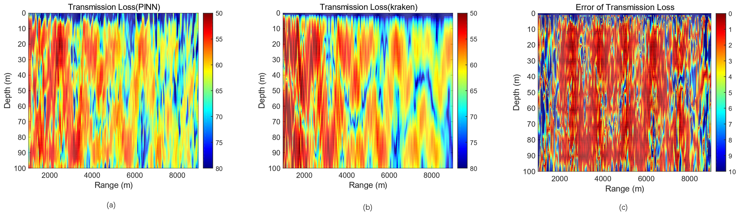
Epoch = 50,000, λMass:λBC:λPDE = 1:1:1, PINN vs. KRAKEN 2D transmission loss pseudo-color maps with errors. (a) PINN forecast result. (b) KRAKEN calculation result. (c) Error between the two results. PINN, physics-informed neural network.
As can be seen from Figure 9c, compared to Figure 7c, the sound field prediction is significantly better, especially at the region where the accurate unlabeled data are not driven, and simply driven by physics alone, it can be seen that when the number of training times is not enough, the model will be underfitted, and it is difficult to predict the accurate results at the prediction place, which puts a higher demand on the computing power of the GPU.
Setting the reception depth to 25, 50, and 75 m plots the PINN prediction against the 1D transmission loss calculated numerically by KRAKEN, as shown in Figure 10.
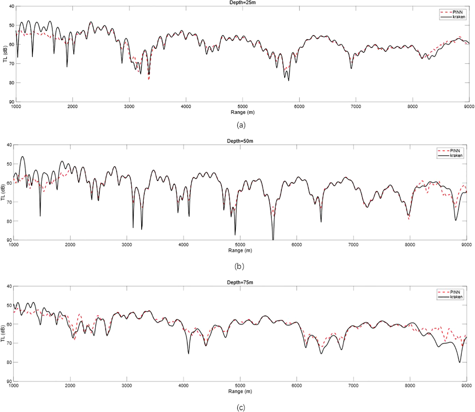
Figure 10
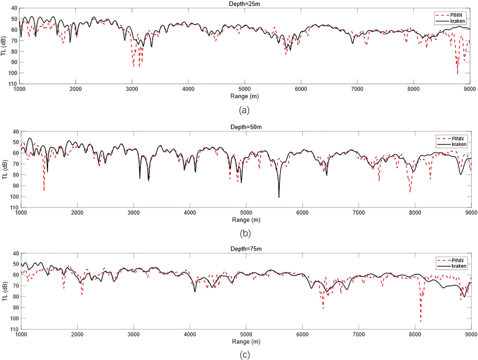
Epoch = 50,000, λMass:λBC:λPDE = 1:1:1, PINN vs. KRAKEN 1D transmission loss. (a) Comparison of 1D transmission loss at a reception depth of 25 m. (b) Comparison of 1D transmission loss at a reception depth of 50 m. (c) Comparison of 1D transmission loss at a reception depth of 75 m. PINN, physics-informed neural network.
As can be seen from Figure 10, compared with Figure 8, the prediction effect of the acoustic field is obviously better; especially at the ranges of 1,000–2,000 and 8,000–9,000 m, the error is obviously reduced, and the prediction accuracy is higher. However, for some extreme points, the model prediction effect is still poor, and it is necessary to gradually adjust the hyperparameters to train a better model to improve the prediction accuracy.
Next, a quantitative error analysis of the 1D transmission loss in Figure 10 is performed to better analyze the experimental results, as shown in Figure 11.
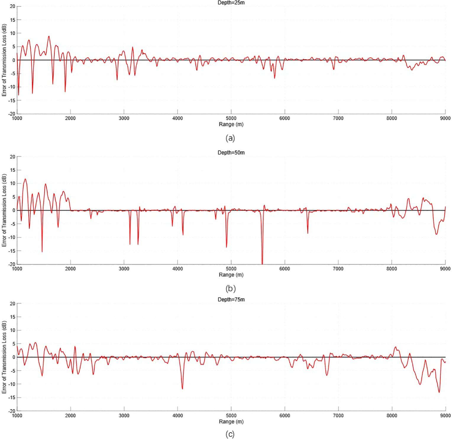
Figure 11
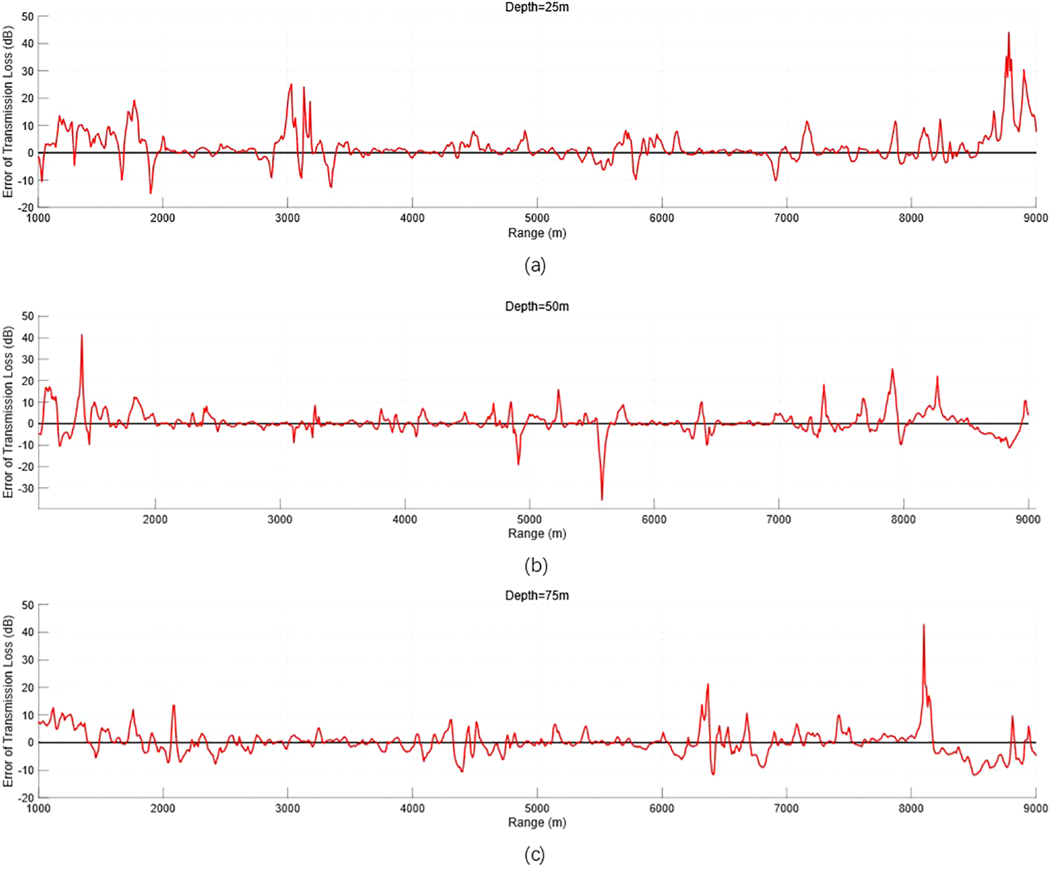
Epoch = 50,000, λMass:λBC:λPDE = 1:1:1, PINN vs. KRAKEN 1D transmission loss error analysis. (a) 1D transmission loss error at a reception depth of 25 m. (b) 1D transmission loss error at a reception depth of 50 m. (c) 1D transmission loss error at a reception depth of 75 m. PINN, physics-informed neural network.
The 1D transmission loss error analysis in Figure 11 is able to analyze the model’s forecasting effect, and the combined analysis with Figure 10 shows that the forecast deviation is larger at some extreme points, which is caused by the neural network’s difficulty in learning for the extreme points, but these extreme points account for a small proportion of the entire range of r. Combined with the needs of the practical application, the transmission loss gap at the vast majority of r is small, and the small undulation is carried out around the 0dB up and down fluctuations, proving the effectiveness of the model, which can be used for sound field prediction.
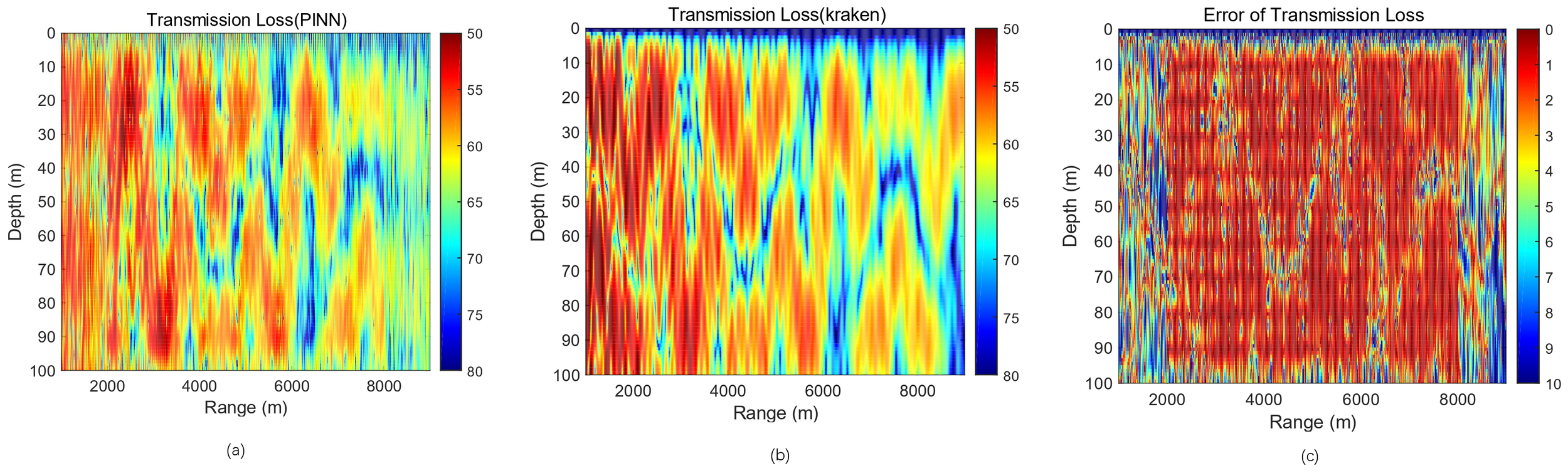
In the actual training process, we found that the size of is always about two orders of magnitude smaller than and , so when synthesizing the total loss function in Equation 14, the is easily overwhelmed by the other two terms because it is too small to be of much use. Therefore, we try to set the ratio of the three loss functions to . Other parameters remain unchanged and still train 50,000 times. The model is saved, and a forecast is made, as shown in Figure 12, plotting the PINN forecast against the KRAKEN numerically calculated 2D transmission loss.
Figure 12
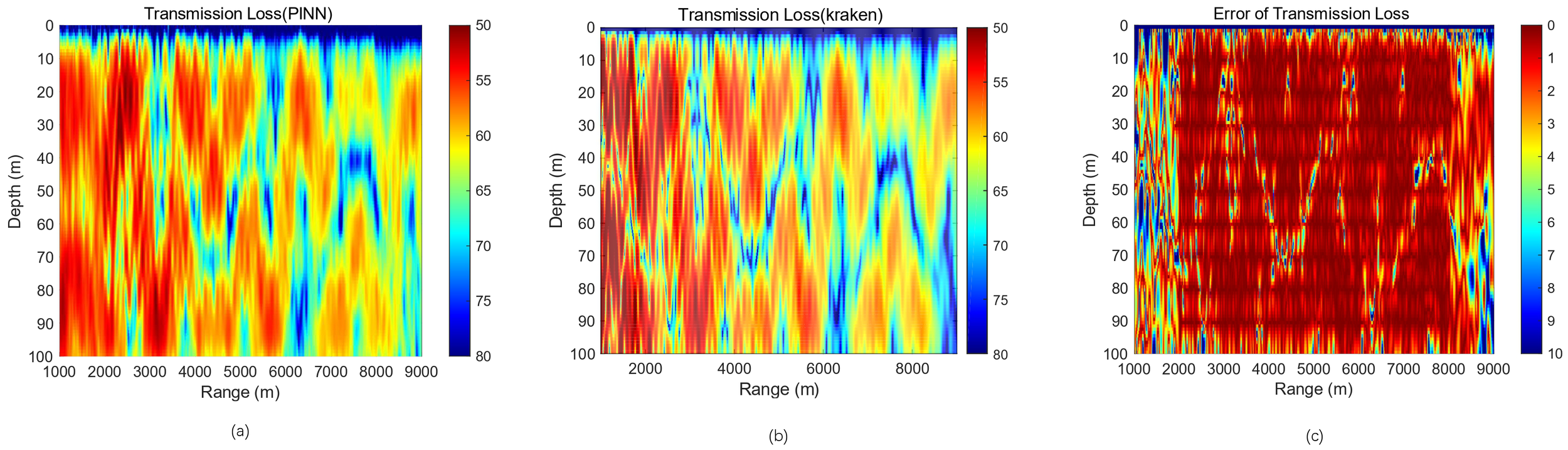
Epoch = 50,000, λMass:λBC:λPDE = 1:1:100, PINN vs. KRAKEN 2D transmission loss pseudo-color maps with errors. (a) PINN forecast result. (b) KRAKEN calculation result. (c) Error between the two results. PINN, physics-informed neural network.
As can be seen from Figure 12c, compared to Figure 9c, the sound field prediction becomes significantly better, especially at the region where no accurate unlabeled data drive is performed, and the region is simply driven by the physical drive alone, which can be seen that when adjusting the ratio between the three loss functions, the role of the is more clearly demonstrated, and the training of the internal random sampling points is more effective.
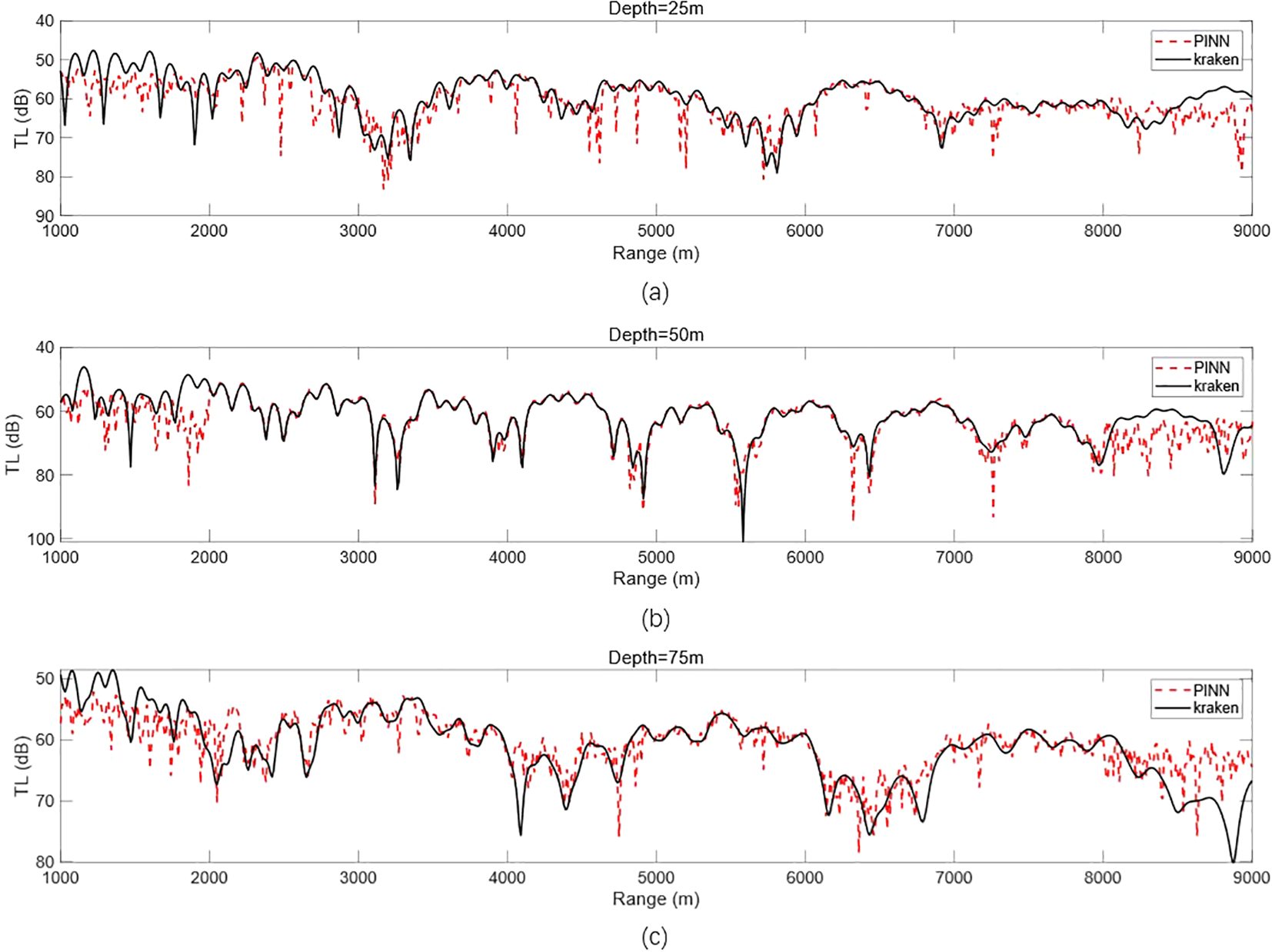
Setting the reception depth to 25, 50, and 75 m plots the PINN prediction against the 1D transmission loss calculated numerically by KRAKEN, as shown in Figure 13.
Figure 13
Epoch = 50,000, λMass:λBC:λPDE = 1:1:100, PINN vs. KRAKEN 1D transmission loss. (a) Comparison of 1D transmission loss at a reception depth of 25 m. (b) Comparison of 1D transmission loss at a reception depth of 50 m. (c) Comparison of 1D transmission loss at a reception depth of 75 m. PINN, physics-informed neural network.
As can be seen from Figure 13, compared with Figure 10, the prediction effect of the acoustic field is obviously better; especially in r ranges of 1,000–2,000 and 8,000–9,000 m, the error is obviously reduced, and the prediction accuracy is higher. However, for some extreme points, the model prediction effect is still poor, and it is necessary to gradually adjust each hyperparameter to train a better model to improve the prediction accuracy.
The variation of errors with propagation distance follows the acoustic propagation law of “near-field mode excitation–mid-field stable propagation–far-field energy attenuation” and forms a cross-influence with errors in the depth dimension:
1. Near field (1,000–2,000 m): incomplete mode excitation and dynamics signal adjustment.
The near field is the excitation stage of normal modes, where the number of modes gradually increases from partial excitation to the full order (15 orders), and the signal fluctuation law changes continuously. However, PINN training relies on mid-field stable mode data, and its generalization ability for near-field dynamics signals is insufficient. Meanwhile, multipath interference in the near field is stronger, further amplifying the error.
2. Mid field (2,000–8,000 m): stable modes and gentle attenuation, minimum error.
The mid-field is the stable propagation stage of normal modes. All 15 orders of modes are excited with fixed energy proportions, and sound waves propagate in the form of stable modal superposition. Energy attenuation only follows the spherical wave law, with a gentle rate and stable signal-to-noise ratio (SNR). This stable physical process is fully compatible with the learning characteristics of PINN, so the error at all depths in this interval is the smallest.
3. Far field (8,000–9,000 m): cumulative energy attenuation and difficulty in capturing weak signals.
The far field is the energy attenuation stage of normal modes. In addition to spherical wave attenuation, the volume absorption effect of seawater emerges, causing the signal SNR to decrease significantly, below the threshold for effective fitting by PINN. Meanwhile, the energy proportion of high-order modes drops sharply, reducing the “modal diversity” of the signal. PINN is prone to the problem of gentle gradients when fitting weak signals + low-frequency fluctuations, leading to a slight increase in error.
Next, a quantitative error analysis of the 1D transmission loss in Figure 13 is performed to better analyze the experimental results, as shown in Figure 14.
Figure 14
Epoch = 50,000, λMass:λBC:λPDE = 1:1:100, PINN vs. KRAKEN 1D transmission loss error analysis. (a) 1D transmission loss error at a reception depth of 25 m. (b) 1D transmission loss error at a reception depth of 50 m. (c) 1D transmission loss error at a reception depth of 75 m. PINN, physics-informed neural network.
The 1D transmission loss error analysis in Figure 14 is able to analyze the forecasting effect of the model, and the combination of the analysis with Figure 13 shows that the forecast deviation is larger at some extreme points, which is caused by the difficulty of the neural network to learn the extreme points, but these extreme points account for a small percentage in the whole range, and in combination with the practical application requirements, the transmission loss gap at the vast majority of the points is small, and small ups and downs are carried out around 0-dB fluctuations, proving the effectiveness of the model, which can be used for sound field prediction.
To intuitively quantify the prediction accuracy of PINN, under the experimental conditions of Epoch = 50 000 and loss weight ratio , four core indicators are selected: RMSE, mean absolute error (MAE), mean relative error (MRE), and correlation coefficient (R). These indicators are used to compare the predicted values of PINN with the numerical solutions (ground truth) of KRAKEN. The following sections first clarify the definition and calculation formulas of each indicator, then present quantitative results in Table 2, and finally analyze the significance of the indicators.
Table 2
| Training epoch | Receiver depth | RMSE (dB) | MAE (dB) | MRE (%) | Correlation coefficient (R) |
|---|---|---|---|---|---|
| 12,000 | 25 m | 2.8 | 2.1 | 7.2 | 0.86 |
| 50 m | 1.3 | 0.9 | 3.5 | 0.94 | |
| 75 m | 2.5 | 1.9 | 6.0 | 0.88 | |
| Full-depth average | 2.2 | 1.7 | 5.6 | 0.90 | |
| 50,000 | 25 m | 1.6 | 1.2 | 4.0 | 0.93 |
| 50 m | 0.7 | 0.5 | 2.0 | 0.98 | |
| 75 m | 1.4 | 1.0 | 3.5 | 0.95 | |
| Full-depth average | 1.2 | 0.9 | 3.2 | 0.96 |
Quantitative error results from training epoch.
RMSE, root mean square error; MAE, mean absolute error; MRE, mean relative error.
All indicators are calculated based on transmission loss. The sample statistical rules are as follows:
-
Single depth (25/50/75 m): The calculation interval covers the propagation distance from 1,000 to 9,000 m, with a total of 801 sample points, and the sample size N = 801.
-
Full-depth average: The average of indicators for nine depths from 10 to 90 m (with an interval of 10 m) is calculated, and the sample size for each depth is 801.
The specific calculation formulas are as follows:
• RMSE (unit: dB) reflects the overall deviation between predicted values and ground truth; the smaller the value, the higher the accuracy. The calculation formula as shown in Equation 24
where is the th transmission loss value predicted by PINN and is the ith ground truth transmission loss calculated by KRAKEN.
• MAE (unit: dB) reflects the mean absolute deviation between predicted values and ground truth and has strong resistance to extreme value interference. The calculation formula as shown in Equation 25
• MRE (unit: %) reflects the relative proportion of errors (eliminating the influence of TL magnitude), facilitating comparison across depths/distances. The calculation formula as shown in Equation 26
• Correlation coefficient (R) reflects the linear correlation between predicted values and ground truth, with a value range of [0, 1]. The closer it is to 1, the better the fitting consistency. The calculation formula as shown in Equation 27
where is the mean value of TL predicted by PINN and is the mean value of TL calculated by KRAKEN.
The variation of errors with depth is essentially the transmission of sea surface/seabed boundary effects to the model fitting results through signal complexity, specifically manifested as follows:
1. Surface layer at 25 m: multipath interference at the sea surface aggravates signal fluctuation.
At a depth of 25 m, close to the sea surface (only 25 m), sound waves form multipath interference of direct waves and sea surface reflected waves due to the sea surface pressure-release boundary. The acoustic pressure signal after interference exhibits a significant increase in fluctuation frequency and extreme point density, reducing its adaptability to the fully connected layers and activation function of PINN. The network is prone to vanishing gradients for high-frequency non-stationary fluctuations, leading to fitting deviations at extreme points, especially in the near-field region. Additionally, the surface water body is affected by potential wind-wave disturbances, resulting in lower signal phase stability than in the middle layer, further amplifying prediction deviations.
2. Middle layer at 50 m: stable propagation without boundary interference.
At a depth of 50 m, located in the middle of the water body and far from both the sea surface (50 m) and the seabed (including a 20-m sediment interface), it is a “clean area” with minimal boundary interference. The 15th-order normal modes have a uniform energy distribution at this depth, with no obvious modal superposition or cancellation. The acoustic pressure signal fluctuates gently and has a high SNR, fully matching the learning capability of PINN. Therefore, the prediction results at this depth have the highest coincidence with the numerical solution of KRAKEN, and the overall error is the smallest.
3. Bottom layer at 75 m: signal distortion caused by seabed sediments.
At a depth of 75 m, close to the seabed sediment interface (only 25 m), it is significantly affected by the acoustic impedance difference between sediments and water. On the one hand, normal modes (especially high-order ones) undergo modal conversion at the interface, breaking the original energy distribution and causing the signal fluctuation law to deviate from a stable state. On the other hand, sediments have a higher attenuation coefficient, leading to rapid energy loss of sound waves and a decrease in SNR in the far-field region. The combined effect of these two factors increases signal complexity, reducing PINN’s fitting accuracy for weak signals and non-stationary fluctuations.
3.2 Hyperparameter configuration and sensitivity analysis
The hyperparameter configuration of the model in this study is based on the characteristics of the physical problem, literature references, and verification via the control variable method. The core hyperparameters and their selection principles are as follows:
-
Activation function: The sine function () is selected. Referring to the research conclusions of Song et al. (2022), this function exhibits significantly better fitting performance for frequency-domain wavefield PDE problems compared to commonly used functions, such as ReLU and Sigmoid, and can effectively avoid the vanishing gradient problem.
-
Optimizer and learning rate: The Adam optimizer (with a learning rate of 0.001) is adopted, which is widely used in deep learning for solving PDE problems (Raissi et al., 2019). Pre-experiment verification shows that when the learning rate is higher than 0.01, training tends to oscillate and diverge; when the learning rate is lower than 0.0001, the convergence speed is extremely slow (stable error cannot be achieved even after 50,000 iterations).
-
Network structure parameters: For the number of hidden layers () and the number of neurons per layer (), combinations of and are tested using the control variable method. When , the model’s fitting ability is insufficient; when or , the model exhibits overfitting. The configuration of five hidden layers with 100 neurons achieves an optimal balance between accuracy and generalization ability.
-
Loss function weights: The selection of the core hyperparameter needs to balance data fitting and physical constraints, and its sensitivity will be analyzed in detail in the following content.
Four groups of comparative experiments are designed (50,000 training epochs) to test the impact of different weight ratios on model performance.
The results are shown in Table 3.
Table 3
| RMSE (dB) | MAE (dB) | |
|---|---|---|
| 1:1:1 | 2.3 | 1.8 |
| 1:1:50 | 1.7 | 1.3 |
| 1:1:100 | 1.2 | 0.9 |
| 1:1:200 | 1.9 | 1.5 |
Results of loss weight sensitivity analysis.
RMSE, root mean square error; MAE, mean absolute error.
When , the physical constraint term is “overwhelmed” by the data term and boundary term, making it difficult for the model to learn the physical laws of acoustic propagation, and the error increases significantly. When , the model achieves optimal performance: the RMSE and MAE are the smallest, the convergence speed is the fastest, and the physical constraint can fully exert its effect without excessively suppressing data fitting. When the excessively high weight of the physical constraint causes the model to overemphasize satisfying the elliptic fluctuation equation, leading to increased deviation from real sound field data and decreased convergence stability.
3.3 Comparative experiments with other neural network methods
To verify the core advantage of physical constraints in the PINN, two typical pure data-driven models are selected for comparison:
-
Comparative Model 1—standard feedforward ANN: It has the same structure as the PINN in this study (5 hidden layers + 100 neurons + sine activation function), but the physical constraint term is removed (the loss function only retains ).
-
Comparative Model 2—convolutional neural network (CNN): It adopts a structure of “3 convolutional layers + 2 fully connected layers”. The input is the encoded feature of coordinates, with no physical constraints, and the sound field mapping relationship is learned only through data-driven methods.
The number of training epochs is uniformly set to 50,000, and hyperparameters (learning rate, batch size, and activation function) remain consistent; the only difference lies in whether physical constraints are introduced.
The evaluation indicators are shown in Table 4.
Table 4
| Model | RMSE (dB) | MAE (dB) | MRE (%) | R |
|---|---|---|---|---|
| Proposed PINN (with physical constraints) | 1.2 | 0.9 | 3.2 | 0.96 |
| Standard ANN (without physical constraints) | 3.5 | 2.7 | 9.8 | 0.7 |
| CNN (without physical constraints) | 2.8 | 2.1 | 7.5 | 0.78 |
Comparison of quantitative indicators among different models.
RMSE, root mean square error; MAE, mean absolute error; MRE, mean relative error; PINN, physics-informed neural network; ANN, artificial neural network; CNN, convolutional neural network.
Based on the comparative data in Table 4, the PINN model with physical constraints is comprehensively superior to purely data-driven models such as standard feedforward neural networks and convolutional neural networks in key performance indicators of underwater acoustic field prediction. From the perspective of error control, the RMSE, MAE, and MRE of the PINN are all significantly lower than those of the two types of purely data-driven models, reflecting its more accurate fitting of acoustic field propagation laws and stronger error stability. In contrast, purely data-driven models, due to the lack of constraints from acoustic physical laws, are prone to fitting deviations in complex acoustic field environments, resulting in higher values of various error indicators. From the perspective of fitting consistency, the correlation coefficient of the PINN is much higher than that of purely data-driven models and much closer to the ideal value of 1, indicating a higher degree of consistency between its predicted results and the real acoustic field, as well as its ability to more accurately replicate the intrinsic characteristics of acoustic field propagation.
This data comparison clearly confirms the key role of physical constraints: by integrating physical priors from the elliptic fluctuation equation, boundary conditions, and relevant acoustic theories, the PINN effectively compensates for the shortcomings of purely data-driven models, which rely on statistical features and lack physical logic guidance. This enables the PINN to maintain excellent prediction performance even in complex acoustic field scenarios, fully highlighting the performance advantages of the proposed PINN framework compared to purely data-driven methods.
4 Conclusions and discussions
4.1 Conclusions
Based on the experimental results in Section 4, we obtain the following experimental conclusions:
-
The PINN structure is highly dependent on partially exact solutions as labeled data and must be adapted for complex ocean dynamics modeling problems that are difficult to learn for deep physical processes using only a simple fully connected layer structure.
-
In the deep learning process, hyperparameters have a great impact, such as the learning rate, the type of optimizer used, the activation function used, the number of hidden layers, the number of neurons in each layer, and some specific hyperparameters in the structure of the PINN, such as the weight of the loss function , have an important impact on the forecasting effect of the trained model and its applicability and need to be adjusted for many attempts.
-
During training, if the number of training rounds is low, there may be underfitting; the trained model is simpler and performs poorly on both the training and test sets. If the number of training rounds is too high, there may be overfitting; the model generalizes poorly and performs poorly on the test set.
4.2 Discussions
In view of the above experimental conclusions, we propose several discussions:
-
For the specific problem of sound field prediction, it is necessary to use some network structures that can be improved by extracting the features of the data using a small amount of labeled data. For example, Hu et al. (2023) proposed an augmented physics-informed neural network (APINN) based on region decomposition and parameter sharing strategy, which improved the efficiency and effectiveness of PINN in dealing with complex partial differential equations. Zeng et al. (2022) proposed a competitive physics-informed neural network (CPINN) based on reinforcement learning in adversarial ideas, which trained a discriminative network specifically scored for the errors generated by the PINN, which has significantly improved the robustness of the algorithm itself.
-
For the problem that hyperparameters have a large impact on the network, it is necessary to use the method of control variables and combine it with the experience of researchers in the references for tuning parameters for a specific problem, adjusting one hyperparameter at a time until the most suitable hyperparameters are tried out in combination. Some adaptive tuning algorithms can also be adopted to adjust the hyperparameters. For example, Wang et al. (2021) proposed a learning rate annealing algorithm to solve the problem of unstable imbalance in gradient size during gradient descent.
-
For the overfitting and underfitting problems in the training process, it is necessary to print out and save the changes in the loss function in time during the training process; according to the trend of its changes, it is necessary to stop early in the case where the loss function is just converged and the fitting effect is better without overfitting, and it is necessary to use the validation set to assist in the training if necessary.
Statements
Data availability statement
The original contributions presented in the study are included in the article/supplementary material. Further inquiries can be directed to the corresponding author.
Author contributions
LC: Writing – original draft. LZ: Writing – review & editing. XS: Conceptualization, Writing – review & editing. JD: Data curation, Writing – review & editing. LY: Investigation, Writing – review & editing. XZ: Methodology, Writing – review & editing. JC: Software, Writing – review & editing.
Funding
The author(s) declare that no financial support was received for the research and/or publication of this article.
Acknowledgments
The authors would like to thank SPIB (Signal Processing Information Base), where the related data originally come from.
Conflict of interest
The authors declared that this work was conducted in the absence of any commercial or financial relationships that could be construed as a potential conflict of interest.
Generative AI statement
The author(s) declare that Generative AI was not used in the creation of this manuscript.
Any alternative text (alt text) provided alongside figures in this article has been generated by Frontiers with the support of artificial intelligence and reasonable efforts have been made to ensure accuracy, including review by the authors wherever possible. If you identify any issues, please contact us.
Publisher’s note
All claims expressed in this article are solely those of the authors and do not necessarily represent those of their affiliated organizations, or those of the publisher, the editors and the reviewers. Any product that may be evaluated in this article, or claim that may be made by its manufacturer, is not guaranteed or endorsed by the publisher.
Abbreviations
PINN, physics-informed neural network; WE, wave equation; HE, Helmholtz equation; WI, wavenumber integration; NM, normal mode; PE, parabolic equation; PDE, partial differential equation; FDM, finite difference method; FEM, finite element method; FVM, finite volume method; BEM, boundary element method; DeepONet, Deep Operator Network; FNO, Fourier Neural Operator.
References
1
Collis J. M. Siegmann W. L. Jensen F. B. Zampolli M. Küsel E. T. Collins M. D. (2008). Parabolic equation solution of seismo-acoustics problems involving variations in bathymetry and sediment thickness. J. Acoustical Soc. America123, 51–55. doi: 10.1121/1.2799932
2
Cybenko G. (1989). Approximation by superpositions of a sigmoidal function. Mathematics control signals Syst.2, 303–314. doi: 10.1007/BF02551274
3
Dean J. Monga R. (2015). TensorFlow Large-scale machine learning on heterogeneous distributed systems. Available online at: TensorFlow.org.
4
Du L. Wang Z. Lv Z. Wang L. Han D. (2023). Research on underwater acoustic field prediction method based on physics-informed neural network. Front. Mar. Sci.10, 1302077. doi: 10.3389/fmars.2023.1302077
5
Duan J. Zhao H. Song J. (2024). Spatial domain decomposition-based physics-informed neural networks for practical acoustic propagation estimation under ocean dynamics. J. Acoustical Soc. America155, 3306–3321. doi: 10.1121/10.0026025
6
Fogarty T. R. LeVeque R. J. (1999). High-resolution finite-volume methods for acoustic waves in periodic and random media. J. Acoustical Soc. America106, 17–28. doi: 10.1121/1.428038
7
Gao Y. Xiao P. Li Z. (2024). “ Physics-informed neural networks for solving underwater two dimensional sound field,” in 2024 OES China Ocean Acoustics (COA). 1–4 ( IEEE).
8
Godin O. (1992). Theory of sound propagation in layered moving media. J. Acoustical Soc. America92, 3442–3442. doi: 10.1121/1.404150
9
Han J. Jentzen A. E W. (2018). Solving high-dimensional partial differential equations using deep learning. Proc. Natl. Acad. Sci.115, 8505–8510. doi: 10.1073/pnas.1718942115
10
Hornik K. Stinchcombe M. White H. (1989). Multilayer feedforward networks are universal approximators. Neural Networks2, 359–366. doi: 10.1016/0893-6080(89)90020-8
11
Hu Z. Jagtap A. D. Karniadakis G. E. Kawaguchi K. (2023). Augmented physics-informed neural networks (apinns): A gating network-based soft domain decomposition methodology. Eng. Appl. Artif. Intell.126, 107183. doi: 10.1016/j.engappai.2023.107183
12
Huang Z. An L. Ye Y. Wang X. Cao H. Du Y. et al . (2024). A broadband modeling method for range-independent underwater acoustic channels using physics-informed neural networks. J. Acoustical Soc. America156, 3523–3533. doi: 10.1121/10.0034458
13
Jensen F. B. Kuperman W. A. Porter M. B. Schmidt H. Tolstoy A. (2011). Computational ocean acoustics Vol. 2011 ( Springer).
14
Li K. Chitre M. (2023). Data-aided underwater acoustic ray propagation modeling. IEEE J. Oceanic Eng.48, 1127–1148. doi: 10.1109/JOE.2023.3292417
15
Li Z. Kovachki N. Azizzadenesheli K. Liu B. Bhattacharya K. Stuart A. et al . (2020). Fourier neural operator for parametric partial differential equations. arXiv preprint arXiv:2010.08895.
16
Liu W. Zhang L. Wang Y. Cheng X. Xiao W. (2021). A vector wavenumber integration model of underwater acoustic propagation based on the matched interface and boundary method. J. Mar. Sci. Eng.9, 1134. doi: 10.3390/jmse9101134
17
Lu L. Jin P. Karniadakis G. E. (2019). Deeponet: Learning nonlinear operators for identifying differential equations based on the universal approximation theorem of operators. arXiv preprint arXiv:1910.03193.
18
Lu Y. Zhang H. Pan X. (2008). Numerical simulation of flow-field and flow-noise of a fully appendage submarine. J. Vibration Shock27, 142–146.
19
Ma Y. Yu D. Wu T. Wang H. (2019). Paddlepaddle: An open-source deep learning platform from industrial practice. Front. Data Domputing1, 105–115.
20
Mallik W. Jaiman R. K. Jelovica J. (2022). Predicting transmission loss in underwater acoustics using convolutional recurrent autoencoder network. J. Acoustical Soc. America152, 1627–1638. doi: 10.1121/10.0013894
21
Paszke A. (2019). Pytorch: An imperative style, high-performance deep learning library. arXiv preprint arXiv:1912.01703.
22
Pekeris C. L. (1948). Theory of propagation of explosive sound in shallow water. doi: 10.1130/MEM27
23
Porter M. B. (1992). The kraken normal mode program.
24
Raissi M. Perdikaris P. Karniadakis G. E. (2019). Physics-informed neural networks: A deep learning framework for solving forward and inverse problems involving nonlinear partial differential equations. J. Comput. Phys.378, 686–707. doi: 10.1016/j.jcp.2018.10.045
25
Schmidt H. Glattetre J. (1985). A fast field model for three-dimensional wave propagation in stratified environments based on the global matrix method. J. Acoustical Soc. America78, 2105–2114. doi: 10.1121/1.392670
26
Song C. Alkhalifah T. Waheed U. B. (2022). A versatile framework to solve the helmholtz equation using physics-informed neural networks. Geophysical J. Int.228, 1750–1762. doi: 10.1093/gji/ggab434
27
Stephen R. A. (1988). A review of finite difference methods for seismo-acoustics problems at the seafloor. Rev. Geophysics26, 445–458. doi: 10.1029/RG026i003p00445
28
Thompson L. L. (2006). A review of finite-element methods for time-harmonic acoustics. J. Acoustical Soc. America119, 1315–1330. doi: 10.1121/1.2164987
29
Tu H. Wang Y. Yang C. Liu W. Wang X. (2023). A chebyshev–tau spectral method for coupled modes of underwater sound propagation in range-dependent ocean environments. Phys. Fluids35. doi: 10.1063/5.0138012
30
Wang S. Teng Y. Perdikaris P. (2021). Understanding and mitigating gradient flow pathologies in physics-informed neural networks. SIAM J. Sci. Computing43, A3055–A3081. doi: 10.1137/20M1318043
31
Zeng Q. Kothari Y. Bryngelson S. H. Schäfer F. (2022). Competitive physics informed networks. arXiv preprint arXiv:2204.11144.
Summary
Keywords
wave equation, KRAKEN, envelope function, PINN, sound field prediction
Citation
Chen L, Zhang L, Sun X, Duan J, Yin L, Zheng X and Chen J (2025) Research on intelligent predicting method of underwater acoustic field based on physics-informed neural network. Front. Mar. Sci. 12:1665305. doi: 10.3389/fmars.2025.1665305
Received
14 July 2025
Revised
19 November 2025
Accepted
21 November 2025
Published
18 December 2025
Volume
12 - 2025
Edited by
Chunyan Li, Louisiana State University, United States
Reviewed by
Tianyu Zhang, Guangdong Ocean University, China
Zhengyu Hou, Sun Yat-sen University, China
Updates
Copyright
© 2025 Chen, Zhang, Sun, Duan, Yin, Zheng and Chen.
This is an open-access article distributed under the terms of the Creative Commons Attribution License (CC BY). The use, distribution or reproduction in other forums is permitted, provided the original author(s) and the copyright owner(s) are credited and that the original publication in this journal is cited, in accordance with accepted academic practice. No use, distribution or reproduction is permitted which does not comply with these terms.
*Correspondence: Lei Chen, chenlei00430@163.com
Disclaimer
All claims expressed in this article are solely those of the authors and do not necessarily represent those of their affiliated organizations, or those of the publisher, the editors and the reviewers. Any product that may be evaluated in this article or claim that may be made by its manufacturer is not guaranteed or endorsed by the publisher.