Abstract
Introduction and Methods:
Field observations were conducted on an intertidal mudflat along the Zhejiang coast to investigate the influence of tidal surges and waves on subtidal sediment flux. This study reveals a two-layer structure in subtidal sediment flux: landward flux occurs above the mid-depth of the water column, while seaward flux is observed in the near-bed layer.
Results:
Strong tidal surges were observed at both the beginning and end of tidal cycles, enhancing sediment transport. Wave height and mean wave periods peaked during high tide and decreased during tidal surges. In the water column layers above mid-depth, flood surges with high suspended sediment concentrations (SSC) induced landward sediment flux in the subtidal time scale. In the near-bed layer, SSC exhibited peaks during flood surges, ebb surges, and high tide.
Discussion:
During high tide, upward diffusion of sediment by tidal currents balances the downward sediment setting at the near-bed layer, promoting the accumulation of sediment setting from upper layer. The wave shear stress suspended the seabed sediment during high tide, facilitating the formation of near-bed high SSC. Tidal currents showed shorter durations during the flood phase and longer durations during the ebb phase. The high SSC transported seaward by weak ebb currents during high tide accounted for approximately 30% of the total ebb sediment flux, playing a significant role in offshore subtidal sediment transport. The macrotides and strong wave activity provide suitable condition for the development of the two-layer structure of sediment transport in intertidal mudflats.
Highlights
-
Subtidal sediment flux across an intertidal mudflat has a two-layered structure
-
Flood surges give rise to the subtidal landward sediment flux in the middle and upper layers.
-
Wave-enhanced bottom shear stress, tidal current diffusion and sediment settling generates the high sediment concentration during high tide.
1 Introduction
Intertidal flats are dynamic zones situated between mean high and mean low tide levels, serving as essential interfaces between terrestrial and marine environments. These areas play a critical role in the global material cycles by facilitating exchanges of sediments, nutrients, and other substances between the sea and land (e.g., Le Hir et al., 2000; Cook et al., 2004a, 2004b; Chen et al., 2022). Intertidal flats also support a rich diversity of benthic fauna and fish species, offering unique habitats (Foster et al., 2013; Barbier, 2013; Dyer et al., 2000), and are vital feeding grounds for migratory and wintering birds (Andersen et al., 2010; Ysebaert et al., 2003). Furthermore, these areas provide natural coastal protection by attenuating the impacts of storms and stabilizing shorelines, acting as buffers that dissipate tidal and wave energy within the near-shore zone (Bale et al., 2006; Costanza et al., 2008; Gedan et al., 2011; Temmerman et al., 2012).However, intertidal mudflats are undergoing substantial decline due to a combination of coastal development, diminished sediment supply from major rivers (e.g., Chung et al., 2004; French et al., 2000; Wang et al., 2012), delta subsidence, increased coastal erosion, and rising sea levels (e.g., Feng and Tsimplis, 2014; Möller et al., 2014). Understanding sediment transport dynamics in intertidal flats is critical for predicting long-term shoreline morphological evolution under scenarios of significant natural environmental change and intensified anthropogenic activities. This knowledge is essential for developing strategies that balance the use and conservation of intertidal flats.
The sedimentary processes of erosion, deposition, transport, and mixing in intertidal flats are strongly influenced by the rapidly fluctuating tidal currents and wave dynamics (Janssen-Stelder, 2000; MacVean and Lacy, 2014; Shi et al., 2017; Wang et al., 2006). When tidal forces dominate, sediment transport typically occurs onshore through settling and scouring lag effects (Straaten and Kuenen, 1958; Postma, 1961; Christie et al., 1999). However, the presence of waves significantly alters both the direction and magnitude of sediment transport. Firstly, waves can substantially enhance sediment resuspension. Sanford (1994) demonstrated that wave-induced resuspension is 3 to 5 times more prevalent than tidal resuspension in mud-bottom environments, such as those in upper Chesapeake Bay. Christie et al. (1999) observed an order-of-magnitude increase in suspended sediment concentrations during storm events (wave-dominated conditions) compared to fair weather (tide-dominated conditions) on an intertidal flat in the macrotidal Humber estuary (UK). Similarly, Ralston and Stacey (2007) noted a rapid decline in suspended sediment concentrations in a microtidal intertidal flat in San Francisco Bay (USA) as wind and wave activity diminished. Green et al. (1997) studied a mesotidal intertidal flat at Manukau Harbor (New Zealand), where tidal currents were insufficient to resuspend sediments, with resuspension being entirely governed by episodic wave events. Secondly, a shift in sediment transport direction—from onshore during calm conditions to strongly offshore during storm events—has been observed in numerous intertidal regions. This phenomenon has been documented in the Seine estuary (Le Hir et al., 2000), San Francisco Bay (Ralston and Stacey, 2007; Talke and Stacey, 2008), and the Yangtze River (Yang et al., 2003).
Recent studies have revealed several novel sediment transport processes in intertidal mudflats, based on comprehensive and detailed observational data. Notably, the significance of flood surges during shallow water stages on residual sediment transport and subsequent seabed erosion has been recognized (Zhang et al., 2016; Shi et al., 2017; Zhang et al., 2021). Observations along the Jiangsu coast indicate that surges associated with flood tidal fronts are characterized by pulses of high current velocities and elevated suspended sediment concentrations (SSC), marking the period of most intense sediment transport. When both waves and tides are significant, elevated near-bed SSC has been observed during high tide, as shown by studies on intertidal flats along the Jiangsu coast, China (Wang et al., 2013; Shi et al., 2019), in Brouage, France (Bassoullet et al., 2000), and in the Humber Estuary, UK (Christie et al., 1999). The high SSC observed during high tide is believed to be generated by wave-induced bottom stress. The increased SSC plays a critical role in determining the intensity and direction of subtidal sediment transport, influencing the deposition or erosion processes on intertidal flats. A two-layer structure of subtidal sediment flux has been observed on the intertidal flat along the Jiangsu coast, China (Wang et al., 2012). In this system, fine particles are transported landward within the upper water column by residual currents, while coarser particles are transported seaward within the lower water column. Previous studies have highlighted two commonly occurring phenomena in intertidal mudflats—intense sediment resuspension during tidal surges and high SSC during high tide—when both tidal currents and surface waves are substantial. However, a more thorough investigation into the formation mechanisms of near-bed high SSC during high tide remains absent. Furthermore, sediment movement on intertidal mudflats is often studied by focusing on the near-bed layer or by depth-averaging the entire water column, without addressing the vertical variations in sediment dynamics. Neither of these methods is sufficient to accurately describe sediment transport processes in mudflats, given the vertical gradients in mixing, sediment concentration, and tidal velocities.
The primary objective of this study is to examine the influence of macrotides and significant wave conditions on subtidal sediment flux in an intertidal mudflat environment. We investigate hydrodynamic variables (tidal currents, wave dynamics, and bottom shear stress), sediment concentration, and suspended sediment flux to explore: (a) the mechanisms responsible for the high near-bed sediment concentrations observed during high tide, and (b) the vertical structure of subtidal sediment flux and the factors that govern its distribution. The structure of the paper is as follows: Section 2 describes the field measurements and data processing methods employed in the study. Section 3 presents the key results related to tidal currents, wave characteristics, sediment concentration, and subtidal sediment flux. In Section 4, we discuss the mechanisms and implications of high-sediment-concentration events during high tide. Finally, Section 5 summarizes the main conclusions and highlights their broader implications.
2 Study area and field observations
2.1 Study area
The tidal flats along the Zhejiang coast face directly toward the East China Sea, making them highly susceptible to the combined influence of macrotidal currents and significant wave and swell activity, which contribute to vigorous sediment dynamics. These flats provide an ideal setting for investigating the impact of tidal and wave forces on sediment transport processes. The field study was conducted on the Oufei intertidal mudflat, located between the Oujiang River estuary and the Feiyun River estuary. The surface sediment composition ranges from 3.6% to 5.0% sand, 76.2% to 77.7% silt, and 17.3% to 20.2% clay, with a median grain size (D50) of 14 μm. The mudflat extends 4 to 6 kilometers seaward, exhibiting a gentle slope that varies from 1° in the upper intertidal region to 10° at the outer edge. The intertidal flat is devoid of vegetation and lacks a prominent tidal creek system or significant gullies.
Coastal hydrodynamics in the study area are primarily influenced by a semidiurnal macrotidal regime, with an average tidal range of approximately 4 meters (Wang and Ke, 1997; Xing et al., 2012). Due to the progressively shallowing water depths towards the coastline and the river discharge from the Oujiang River, the M4 tidal component becomes prominent in the nearshore zone, indicating the development of a flood-dominated tidal wave. Swell and surface waves originating from the East China Sea can propagate onto the study mudflats, which are not sheltered by offshore islands. Observations from gauge stations off the Oujiang estuary indicate that the mean wave period ranges from 4 to 10 seconds, with significant wave heights varying between 0.5 meters and 5 meters under typical weather and cold wave conditions (Ye et al., 2022).
2.2 Field observation
The field survey was conducted from 11 to 15 March 2015, spanning six semidiurnal tidal cycles. A variety of time-series data, including water depth, wave level, turbidity, and near-bed velocity, were collected using instruments affixed to a tripod (Figure 1d). The observation site was established in the southern region of a reclamation area, where the sheltered conditions eliminated the alongshore currents at the site (Figures 1b, c).
Figure 1
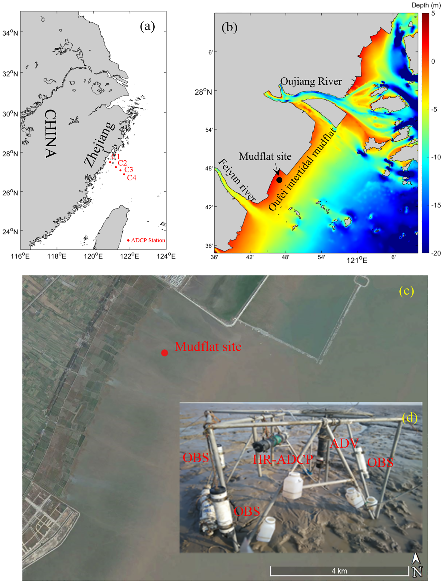
Study area and observation stations. (a) The study area is situated to the south of the Zhejiang coastline, China. (b) The topography of the Zhejiang coastal region is characterized by varied geomorphological features. The primary observation site is located on the Oufei intertidal mudflat, positioned between the Oujiang and Feiyun rivers. Four Acoustic Doppler Current Profiler (ADCP) stations are strategically deployed across the Zhejiang coastal zone for comprehensive monitoring. (c) A satellite image of the Oufei intertidal mudflat is provided, with the mudflat spanning approximately 4 kilometers in width. (d) From 11 March to 15 March 2015, a suite of measurement instruments, including an Optical Backscatter Sensor (OBS), an Acoustic Doppler Velocimeter (ADV), a High-Resolution ADCP (HR-ADCP), and water sampling bottles, were systematically deployed at the intertidal mudflat site to collect in situ data for hydrodynamic and sedimentological analyses.
A 6 MHz Nortek Acoustic Doppler Velocimeter (ADV) was employed to measure high-frequency near-bed velocity and water level variations. The ADV probe was mounted on a tripod, positioned 0.25 m above the seabed, and directed downward at a standoff distance of 0.15 m from the probe head. Consequently, the sample volume of the ADV transducer was located 0.1 m above the bottom (mab). The ADV operated in burst mode at 10-minute intervals, with each burst recording 1000 samples at a frequency of 8 Hz. Velocity profiles were acquired using a downward-looking 2 MHz High-Resolution Acoustic Doppler Current Profiler (HR-ADCP). The HR-ADCP was positioned 0.8 m above the seabed, with velocity data collected in 3 cm bins at a sampling frequency of 1 Hz.
Water turbidity was measured at four vertical layers positioned at 0.1 m, 0.2 m, 0.3 m, and 0.6 m above the seabed using Optical Backscatter Sensors (OBS-3A, self-recording turbidity–temperature monitoring instruments), with a sampling period of 2.5 minutes (Figure 1d). Water samples were simultaneously collected using four custom-made samplers (600 mL volume) placed at the same heights as the OBS-3A sensors to calibrate turbidity measurements, thereby enabling the determination of suspended sediment concentrations.
In order to characterize the tidal currents in the study area, long-term ADCP data were gathered from four mooring stations (C1–C4) along the Zhejiang coast (Figure 1a). The ADCP measurements were conducted between December 2008 and March 2009, along a transect perpendicular to the isobath, covering water depths from approximately 20 m to 70 m. The velocity profile was sampled every 20 minutes, with bin sizes ranging from 0.5 m to 2 m.
3 Method
3.1 Estimation of wave parameters
The significant wave height, Hs, can be estimated from the high-frequency fluctuations in water level recorded by the near-bed ADV. The high-frequency fluctuations of the water level are the difference between the observed water level and the mean water level during a burst. Under the assumption that surface wave heights generally adhere to a Rayleigh distribution, as proposed by Longuet-Higgins (1952), the value of Hs is calculated following the methodology outlined by Wiberg and Sherwood (2008).
where Sη is the spectral density of surface elevation as a function of frequency, f (=1/T).
The mean wave period T is estimated from the spectra of surface elevation as follows (Equation 2):
where the symbols have the same meaning as in Equation 1.
3.2 Wave and turbulence decomposition
Each measured instantaneous velocity (u, v, w) can be considered as the summation of mean flow velocity (, , ), wave oscillatory (, , ), and turbulent (u’, v’, w’) components, indicating (Equation 3)
In general, the turbulent energy spectra within the bottom boundary layer of intertidal mudflats exhibit characteristics consistent with Kolmogorov’s −5/3 law in the inertial subrange. However, wave-induced motion can significantly distort the original turbulent energy spectra in the energy-containing subrange. When wave oscillations are superimposed on turbulent components, the resulting turbulent parameters, such as Reynolds stress and turbulent kinetic energy, may be substantially overestimated.
Several methods have been proposed for separating turbulence and wave-induced fluctuations, including the paired differencing method (Trowbridge, 1998; Shaw and Trowbridge, 2001; Feddersen and Williams, 2007), the cohesive spectral method (Benilov and Filyushkin, 1970; Bendat and Piersol, 2000), and the empirical mode decomposition (EMD) method (Qiao et al., 2016; Bian et al., 2018, 2020). In this study, we employed the cohesive spectral method (Bricker and Monismith, 2007) to identify wave motions by examining the correlations between mutually independent velocity and pressure measurements. The coherence between ADV pressure and high-frequency velocity data (p’ and ui’) was calculated as follows (Equation 4):
where is the cross spectra of and , is the complex conjugate of , and and are power spectra of and , respectively. Then, the power spectra of wave-removed turbulence were obtained following Equation 5
To assess the effectiveness of the wave-removal process, we used velocity bursts from the eastward and vertical components collected during high tide in the second tidal cycle as a case study. The wave-induced peak appears at frequencies lower than 1 Hz (represented by the gray line in Figure 2A), suggesting that the low-frequency band is particularly susceptible to wave fluctuations. For frequencies exceeding 1 Hz, the spectral slope generally adheres to Kolmogorov’s −5/3 law, indicating that the influence of waves on the high-frequency band is negligible. Following the wave-turbulence decomposition procedure, the peaks in the low-frequency band (< 1 Hz) are largely eliminated, with the spectral slope in this range becoming relatively horizontal. Furthermore, the wave-enhanced spectrum exhibits a significantly lower peak in the vertical velocity component compared to the horizontal velocity component (Figure 2B). This finding is consistent with prior research indicating that surface waves have a less pronounced effect on vertical velocity than on horizontal velocity (Stapleton and Huntley, 1995). In accordance with Bricker and Monismith (2007), we assume that waves primarily govern the phase of the Fourier coefficients, as waves dominate velocity fluctuations at the wave crest. The time series of wave oscillations () can be reconstructed by inverse Fourier transform with the modules () of the Fourier coefficients of the wave part and the original phase () by . The corresponding turbulent velocity can be estimated by subtracting the mean flow and wave velocity from the original velocity .
Figure 2
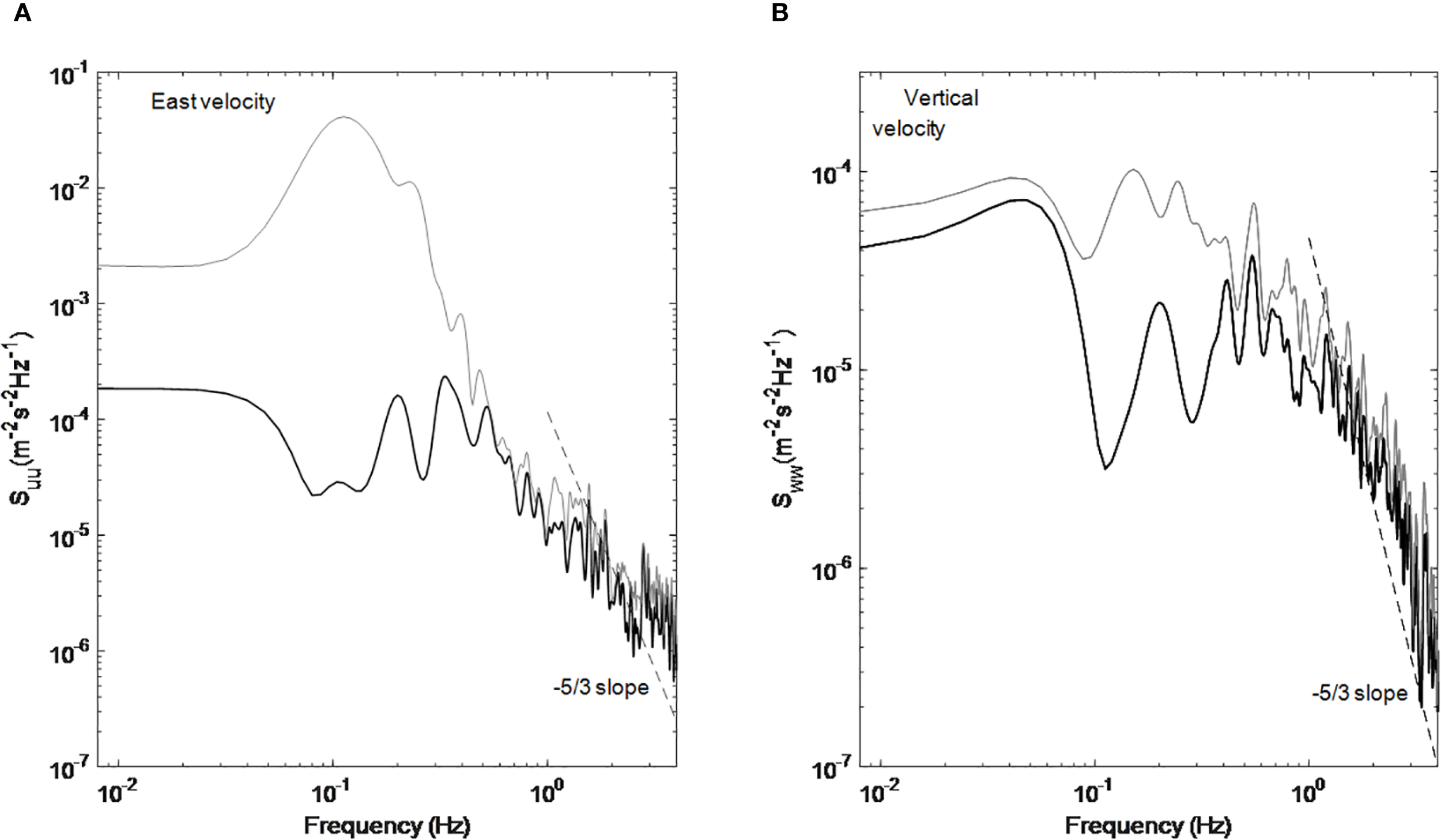
. A comparison of the power spectral density for near-bed ADV velocities (0.1 mab) is presented between the pre-wave (gray line) and post-wave removal (black line) conditions. (A) Spectrum of the eastward velocity burst, and (B) spectrum of the vertical velocity burst, both captured during the second hour of the second semidiurnal tidal cycle. The dashed black line represents the −5/3 spectral slope.
3.3 Estimation of current and wave bottom shear stress
The bottom shear stress due to waves (τw) was estimated according to van Rijn et al. (1993) (Equation 6):
where ρw is seawater density (= 1030 kg m-3). The wave orbital velocity () at the edge of the wave boundary layer is given by (Equation 7)
where ω (= 2π/T) is the angular velocity and is the peak value of the orbital excursion, given by (Equation 8)
where Hs is the significant wave height, h is the water depth, L is the wavelength (= )), g is the gravitational acceleration (9.8 m s-2), and T is the mean period.
Based on Soulsby (1995), the wave friction coefficient fw depends on the hydraulic regime and can be expressed as (Equation 9)
where (= ) is the wave Reynolds number and r (= ) is the relative roughness. For the hydrodynamic condition of the observed intertidal mudflat, has values smaller than ~ 4×10⁴, which indicates a laminar boundary layer induced by waves over the intertidal flat (Jensen et al., 1989).
Since vertical velocity is less affected by surface waves, the bottom shear stress induced by tidal currents (τc, Pa) can be more accurately estimated using near-bed vertical turbulent velocities (Huntley and Hazen, 1988; Kim et al., 2000), as follows (Equation 10):
where C0 is a constant of 0.9, as recommended by Kim et al. (2000). ρ is the seawater density (kg m-3), and is the variance in the vertical turbulent velocity (m2 s-2). w’ is the wave-removed vertical turbulent velocity.
The bed shear stress due to combined current–wave action τcw can be estimated through the van Rijn et al. (1993) model, Soulsby (1995) model, and Grant and Madsen (1979) model. All three models yield very similar results for bed shear stress. Here, we use the Grant and Madsen (1979) model to estimate the current-wave shear stress (Equation 11).
where τw and τc are the bed shear stresses due to waves and currents (N m-2), respectively, and φcw is the angle between the current direction and wave direction. To determine the wave direction, we combine horizontal velocities and pressure data from the ADV using a standard PUV method (available at http://www.nortekusa.com/usa/knowledge-center/table-of-contents/waves) and some MATLAB tools in the Nortek web page that can compute wave directional spectra from data using Nortek Vector. These models have been widely employed in estimating bed shear stress due to current–wave interaction (e.g., Feddersen and Guza, 2003; Keen and Glenn, 2002; Shi et al., 2012; Styles and Glenn, 2002).
The critical shear stress () is essential for evaluating bottom sediment erosion. For cohesive sediments, is primarily governed by cohesive forces resulting from electrochemical interactions between sediment particles, making it challenging to estimate precisely. In this study, we employ two methods to estimate the lower and upper bounds of . The lower band of is determined using the extended Shields curve, as proposed by Mantz (1977) and Govers (1987).
where () is the dimensionless grain size and θcr and τcr are the dimensionless critical shear stress and critical shear stress, respectively. ρ and ρs represent the fluid density (1030 kg m-3) and sediment density (2650 kg m-3), respectively. v is the kinematic viscosity coefficient (=1×10⁻⁶ m2 s-1). g (= 9.8 m s-2) is the gravity acceleration. d50 is the median diameter of the surface sediment and has a value of 12 μm. The upper band of is estimated based on a formula derived from the experimental results of Taki (2000) that is applicable to fine sediments (typically less than several tens of microns) and relatively high-water contents.
3.4 Sediment data
3.4.1 Conversion of turbidity to SSC
Researchers have recognized a strong relationship between turbidity, derived from optical techniques, and suspended sediment concentration (SSC). By utilizing in situ water samples, the correlation between these two variables can be employed to assess SSC variability in the bottom boundary layer (Yuan et al., 2008; Shi et al., 2014). In this study, power-exponential correlations were developed for both the low and high turbidity ranges (Figure 3). The threshold between the low and high turbidity ranges, with values between 200 and 350, was empirically determined based on the goodness of fit. The correlation coefficient between the fitted SSC and the measured SSC is 0.99.
Figure 3
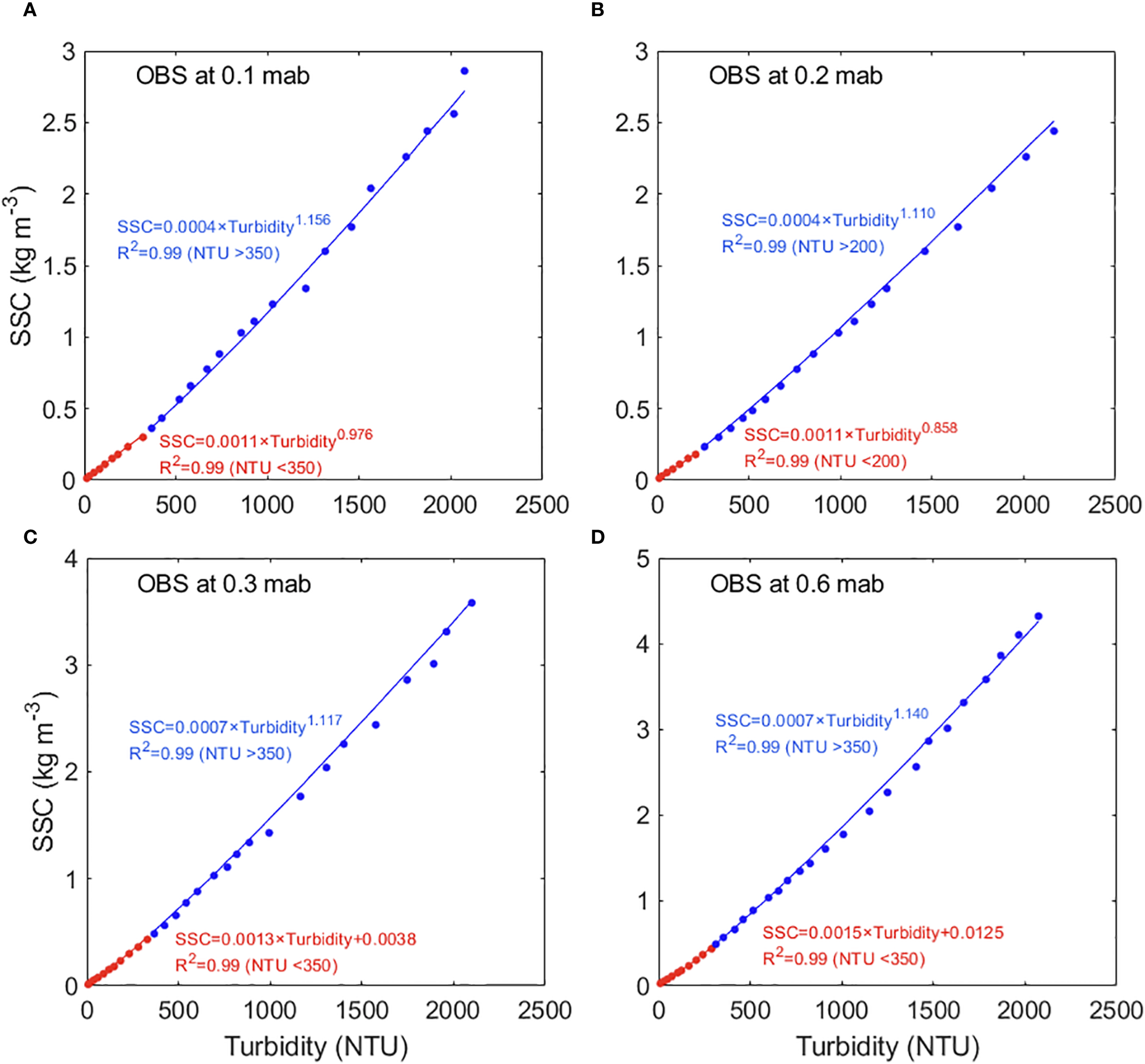
Calibration curves for the Optical Backscatter Sensor (OBS) were obtained through laboratory experiments. Here, OBS refers to the optical backscatter sensor, NTU denotes nephelometric turbidity units, and SSC represents suspended sediment concentration.
3.4.2 Sediment stratification
The magnitude of vertical density stratification was quantified with the Brunt-Väisälä (or buoyancy) frequency, N, defined as (Equation 14)
where g is acceleration due to gravity, ρ0 is the background fluid density (assumed a constant ρ0 = 1020 k gm−3), and z is the vertical coordinate. The density of the water-sediment mixture, , and its vertical gradient were calculated from the SSC data obtained from calibrated turbidity data. is estimated as , where ρs= 2650 kg m-3 is the sediment density.
3.4.3 Sediment diffusivity
For the 0.1 mab layer, sediment diffusion is primarily governed by tidal currents, as the wave-induced bottom boundary layer is too shallow to directly affect vertical sediment diffusion. The layer thickness influenced by both wave and currents is estimated as , where is von Kaman constant, is the bottom shear velocity by currents and waves and is the angular frequency of surface wave (Grant and Madsen, 1986). The thickness is estimated as 0.005 m, much smaller that the layer of ADV measurement. Additionally, the damping effect of near-bottom sediment stratification must be accounted for when estimating sediment diffusivity. Therefore, sediment diffusivity is estimated following Glenn and Grant (1987) (Equation 15):
where u*c is the bottom friction velocity induced by tidal currents, κ (= 0.4) is the von Karman constant, z is the distance from the seabed and L represents the length scale under stratification. γ and β are constants and have values of 0.74 and 4.7, respectively (Glenn and Grant, 1987). In this study, the Ozmidov length scale () was used to describe the stratification effect, where ϵ is the turbulent dissipation rate in W kg-1 and N is the buoyancy frequency in s-1.
The turbulent dissipation rate is estimated using the inertial subrange dissipation method for the ADV (Liu and Wei, 2007; Lozovatsky et al., 2008; Bluteau et al., 2011). When turbulence is fully developed, inertial subranges exist, where energy is transferred from energy-containing eddies to viscous eddies without dissipation. The inertial subrange in the spatial domain is described by Kolmogorov’s first universality hypothesis (Kolmogorov, 1941) (Equation 16).
where E(k) indicates the energy spectral density of the ith turbulent velocity (i = 1, 2, 3) at wavenumber k and ai is a one-dimensional Kolmogorov universal constant. In locally isotropic turbulence, a1 = 0.53 and a2 = a3 = 0.71 (Sreenivasan and Kailasnath, 1993). With Taylor’s frozen hypothesis, the energy spectrum in the spatial domain can be converted to the frequency domain (Equation 17).
where f is the frequency and U is the horizontal mean velocity.
The energy spectrum of Equation 18 can be converted into logarithmic coordinates as:
The vertical velocity is used because it is less affected by surface waves. The dissipation rate can be estimated through the linear fit with a slope of -3/5 to Equation 19. The dissipation rate (ϵ) has the relationship with the intercept of the fitting line (A) as . In our study, dissipation rates with fitting coefficients less than 0.5 or mean velocities less than 0.01 m s-1 are not used.
4 Results
4.1 Water level and tidal currents
The average inundation time at the observation site is approximately 4 hours for each semidiurnal tidal cycle. The M2 semidiurnal tide dominates the variance in water level at the intertidal mudflat, with a maximum water depth of 1.8 m (Figure 4A). The time series of water level during the first two tidal periods clearly exhibit diurnal variations, while the subsequent tidal cycles show nearly equal amplitude (~1.5 m). The rate of water-level change (dη/dt) decreases from the beginning of flood tides to the end of ebb tides. Extremum values are observed at the start and end of each tidal cycle.
Figure 4
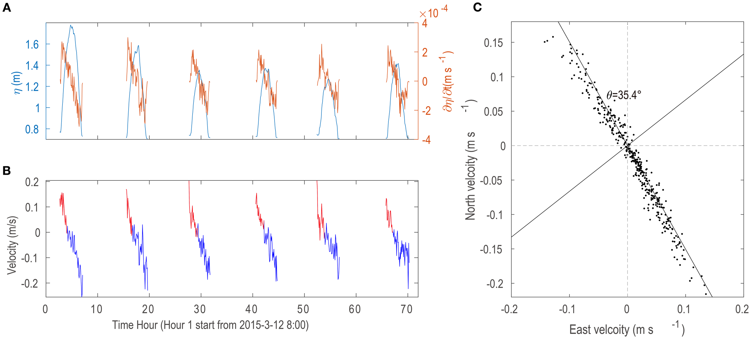
(A) Variation in tidal level for the six semidiurnal tidal cycles observed from 11 March to 15 March 2015. (B) Streamwise velocity recorded by the ADV at 0.1 mab, with positive values (red) representing flood currents and negative values (blue) representing ebb currents. (C) Scatter diagram of eastward and northward velocity components. The primary flow direction of the reversing currents is 35.4° west of north.
Tidal currents on the intertidal mudflat are nearly rectilinear (Figure 4C). The direction of the streamwise velocity axis is 35.4° west of north, almost perpendicular to the shoreline. The velocity along the mudflat is considerably smaller than the velocity across it. Two speed extremes are observed in each semidiurnal tidal cycle when tidal currents flow onto and retreat from the observation station (Figure 4B), indicating the occurrence of strong surges during the very shallow water stages. Surges during such periods have been shown to play a significant role in mudflat sediment transport and bottom erosion (Wang et al., 2013; Shi et al., 2019; Zhang et al., 2021). The average duration of flood currents is 1.4 hours (red segments in Figure 4B), whereas ebb currents have an average duration of 2.7 hours (blue segments in Figure 4B), highlighting tidal asymmetry in flood-ebb duration.
4.2 Temporal variations in surface waves
The maximum significant wave height and the mean wave period during the six semidiurnal tidal cycles are approximately 0.18 m and 6 s, respectively (Figures 5B, C). These two wave parameters exhibit a clear positive correlation with local water depth, gradually increasing from the beginning of the flood tide and decreasing after high tide (Figure 5A). Both wave periods, significant wave height, and maximum wave orbital velocity (Uw) are relatively small during flood and ebb surges. The value of Uw is approximately 0.14 m/s outside of flood and ebb surges and does not exhibit significant peaks during high tide, as Hs and water depth exert opposing effects on Uw (Figure 5D). The intratidal variation in wave parameters suggests that as the tide level rises, the deeper water facilitates the propagation of larger amplitude waves with longer wavelengths onto the observed mudflat. The mudflat of our observation site has flat seabed, which induces the clear relationship between wave parameter and water depth. For complex topography, the wave climates may be complicated due to wave refraction and reflection (Zhu et al., 2024; Gao et al., 2024)
Figure 5
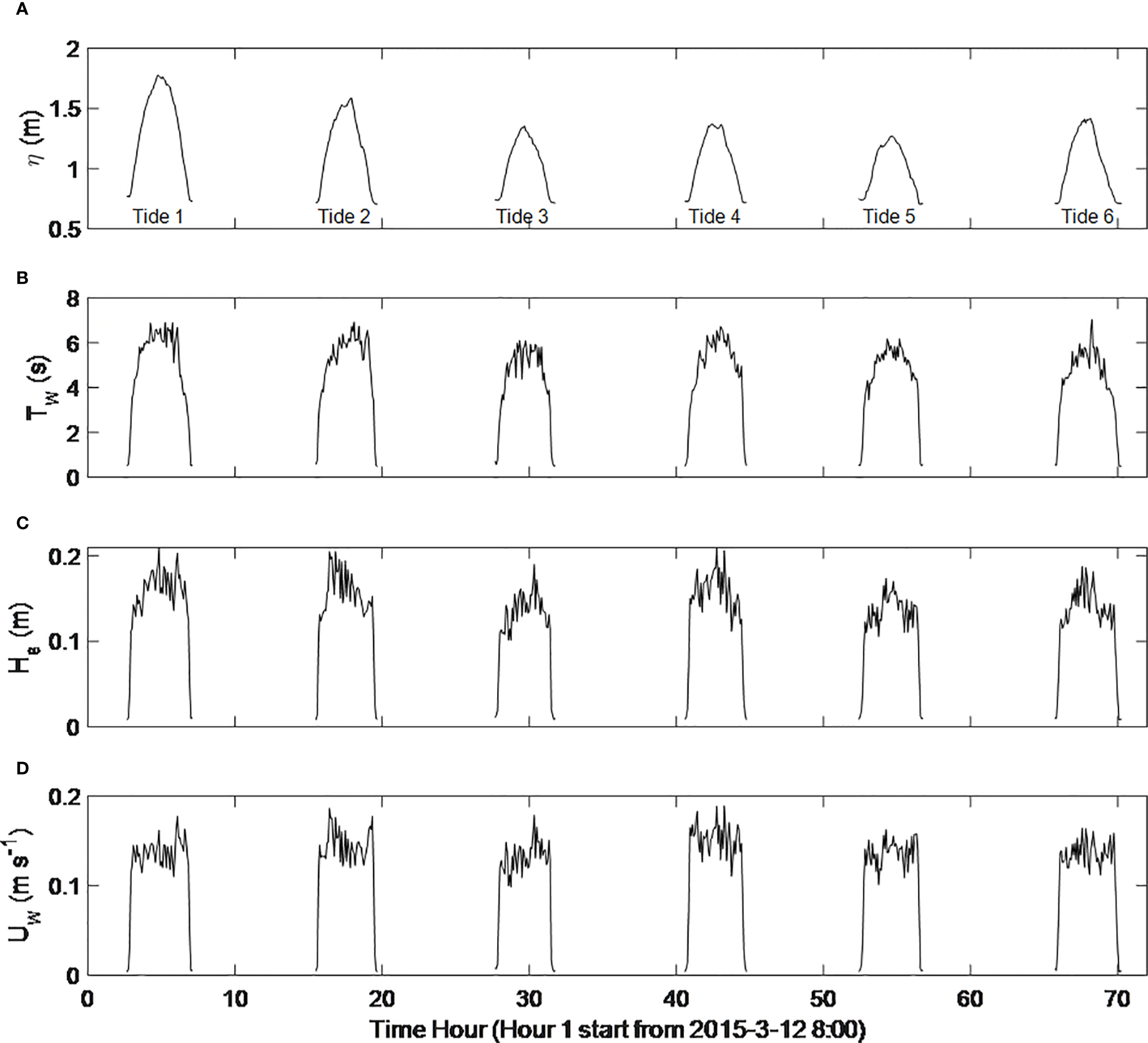
Temporal variation in (A) tidal level (η), (B) mean wave period (Tw), (C) significant wave height (Hs) and (D) bottom orbital velocity (Uw).
4.3 Temporal variation in suspended sediment
The temporal variation in suspended sediment concentration (SSC) in the near-bed layer at 0.1 mab reveals three distinct SSC peaks, occurring at the beginning of the flood tide, the end of the ebb tide, and during high tide (Figures 6A, B). The W-shaped variation in SSC is particularly pronounced in tidal cycles 3, 4, and 5. SSC variation is similar in the 0.2 mab layer, although the concentration during high tide is lower compared to the 0.1 mab layer (Figure 6C). At the 0.3 mab layer, SSC only shows a slight increase during high tide, with extreme SSC values primarily occurring at the beginning of the flood tide and the end of the ebb tide (Figure 6D). The highest SSC at the 0.6 mab layer is observed as the flood tide approaches the observation site. SSC gradually decreases until the end of the ebb tide, without significant high concentrations during high tide (Figure 6E). While Tides 1 and 2 capture the increase in SSC at the end of the ebb tide, this elevated SSC does not develop in subsequent tidal cycles.
Figure 6
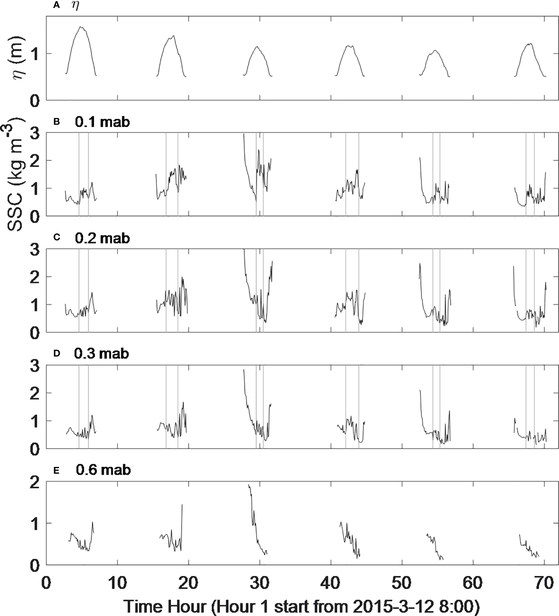
Temporal variation of sea level elevation (A) and suspended sediment concentration (SSC) at (B) 0.1 m above the bottom (mab), (C) 0.2 mab, (D) 0.3 mab, and (E) 0.6 mab.
The elevated SSC at the beginning of the flood tide and the end of the ebb tide may be closely associated with tidal surges, which not only facilitate the horizontal transport of SSC but also significantly resuspend sediment from the seabed. However, no direct evidence exists to confirm the mechanism responsible for the high SSC observed in the near-bed layer during high tide. Given that the mean flow is relatively weak during high tide, horizontal transport is unlikely to account for the observed increase in SSC. The significant SSC during high tide is more likely attributed to either sediment settling from the upper layers or vertical diffusion and resuspension from the lower layers. The occurrence of high SSC during high tide, as observed in this study, is not unique; similar phenomena have been reported in previous studies, such as those conducted on intertidal flats along the Jiangsu coast, China (Wang et al., 2013; Shi et al., 2019), on intertidal mudflats in Brouage, France (Bassoullet et al., 2000), and on intertidal mudflats in the Humber Estuary, UK (Christie et al., 1999).
4.4 Subtidal transport of near-bed sediment
The instantaneous suspended sediment flux per unit width (ISF, kg m−1 s−1) on intertidal flats is the product of the mean velocity and the corresponding instantaneous sediment concentration. The layers at 0.1 mab and 0.6 mab were selected to represent sediment transport in the near-bed and middle layers, respectively. The subtidal sediment flux (SSF) can be estimated as (Equation 20):
where the overbar denotes the tidal-averaged process.
In the middle layer of the water column (0.6 mab), the ISF is most pronounced during flood surges, as maximum tidal currents and elevated SSC occur simultaneously during these periods (Figure 7B). The ISF then decreases substantially and remains at a relatively low level throughout the rest of the tidal cycles. Since high SSC at the end of the ebb tide is not consistently observed in the middle water column, ebb surges do not always lead to significant ISF. Specifically, landward sediment flux is consistently induced by flood surges, while ebb surges may not consistently generate substantial seaward sediment flux to counterbalance the landward transport (Figure 7C). As a result, sediment transport tends to be landward in the 0.6 mab layer due to the tidal asymmetry of SSC on a subtidal time scale.
Figure 7
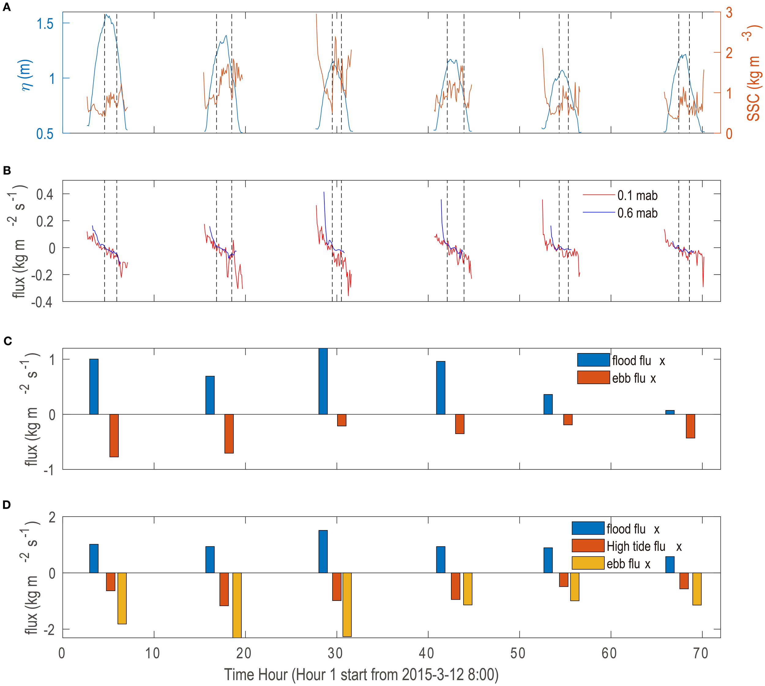
Sediment flux at the 0.6 mab and 0.1 mab layers. (A) Temporal variation in near-bed suspended sediment concentration (SSC) with superimposed tidal levels. Vertical dashed lines indicate the periods of high SSC during high tide. (B) Instantaneous suspended sediment flux (ISF) at 0.6 mab (blue line) and 0.1 mab (red line). (C) Comparison of sediment flux induced by flood and ebb currents at 0.6 mab. (D) Comparison of sediment flux induced by flood and ebb currents at 0.1 mab, with emphasis on the sediment flux during high tide.
In the near-bed layer (0.1 mab), the instantaneous suspended sediment flux (ISF) is significant during both flood and ebb surges. Unlike the 0.6 mab layer, the ISF during flood and ebb surges are nearly balanced. The cumulative effect of ISF during high tide is substantial, despite the weak slack-tide currents. The peak SSC during high tide largely corresponds with ebb currents, leading to seaward sediment flux. To highlight the significance of sediment transport during high tide, the periods of high-water peaks of SSC are indicated by vertical dashed lines in Figures 7A, B. As shown in Figure 7D, sediment flux during high tide significantly contributes to the seaward sediment transport, accounting for approximately 30% of the total seaward flux. In summary, the transport of high SSC with weak ebb currents during high tide promotes seaward subtidal sediment flux. The subtidal sediment flux exhibits a two-layered structure, with the middle and upper layers directed landward, while the near-bed flux is directed seaward.
4.5 Tidal current and wave bottom stress
Sediment resuspension is closely related to bottom shear stress induced by currents and waves. According to Equation 12 and Equation 13, the lower bound of critical shear stress for sediment resuspension is estimated to be 0.0452 Pa, while the upper bound is 0.1 Pa. Significant current-induced bottom shear stress occurs during flood and ebb surges (Figure 8). After these surges, the current-induced bottom shear stress rapidly drops to the lower bound of the critical shear stress for the remainder of the tidal cycles (Figure 8). Due to the low orbital velocity, wave-induced bottom shear stress is minimal during flood and ebb surges (Figure 8). However, during non-surge periods, wave-induced shear stress exceeds the critical shear stress, suggesting that wave-induced shear stress may prevent suspended sediment from settling and can resuspend sediment from the seabed (Figure 8). In general, tidal currents generate high bottom shear stress during flood and ebb surges, while waves play a more significant role in the middle of tidal cycles.
Figure 8
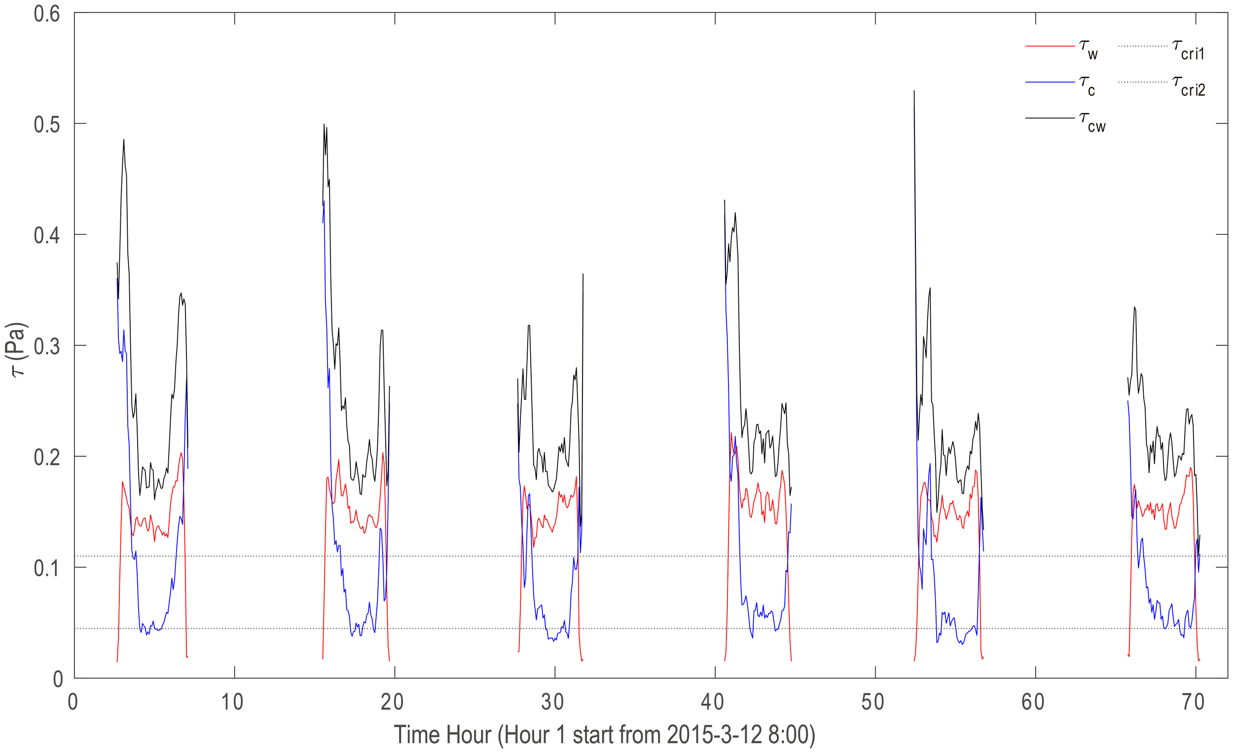
Temporal variation in current-induced bottom shear stress (τc), wave-induced bottom shear stress (τw), and total bottom shear stress (τcw). The critical shear stresses required for sediment suspension are represented by dotted lines.
5 Discussion
Our observations reveal the two-layered structure of subtidal sediment flux in an intertidal mudflat, with landward flux in the upper layer and seaward flux in the bottom layer. Flood surges significantly enhance the development of landward sediment flux in the upper layer, while high SSC events during high tide contribute to the seaward transport of sediment. The asymmetry in tidal duration and the occurrence of high SSC events during high tide are two critical factors influencing the direction and magnitude of sediment transport and warrant further investigation.
5.1 Tidal asymmetry on the intertidal flat
Tidal duration asymmetry has been shown to enhance seaward sediment transport, as the near-bed high SSC during high tide closely aligns with ebb currents. This asymmetry can arise from large-scale influences, such as tide propagation in a shallowing coastal ocean, or from local asymmetries generated by the topography of flat regions (Le Hir et al., 2000). In coastal oceans primarily governed by the M2 semidiurnal tidal cycle, interactions between the M2 and M4 harmonics (2ωM2 = ωM4) are widely recognized as the primary drivers of tidal wave deformation and associated tidal asymmetry (Friedrichs and Aubrey, 1988; Aubrey and Speer, 1985). A phase difference of 2θM2 − θM4 in the range of 0° to 180° results in flood tide dominance, with the flood tide being shorter than the ebb tide, while a phase difference in the range of 180° to 360° leads to ebb tide dominance, with the ebb tide being shorter. A phase difference of exactly 0° or 180° between 2θM2‐θM4 results in equal durations for both flood and ebb tides, thereby eliminating tidal asymmetry, though the wave shape remains statistically skewed. The amplitude ratio AM4/AM2 (where A is tidal amplitude) is used to quantify the magnitude of tidal asymmetry under a given phase difference.
Harmonic analysis was performed on depth-mean velocity series measured by moored Acoustic Doppler Current Profilers (ADCPs) over a 30-day period in the southern Zhejiang coastal ocean, near the observed mudflats (Figure 1). Two indicators were considered: the phase differences and amplitude ratios between the M4 and M2 tidal constituents. The amplitudes and phase angles were calculated using the MATLAB program T_TIDE (Pawlowicz et al., 2002).
The harmonic analysis reveals that the phase difference of 2θM2‐θM4 ranges from approximately 70° to 110°, suggesting a shorter flood duration in the southern Zhejiang coastal ocean. The amplitude ratio between the M4 and M2 tidal constituents increases significantly from offshore to nearshore (Table 1), indicating that the nonlinear effects of tidal currents intensify as water depth decreases. Tidal asymmetries established offshore of the Zhejiang coast directly contribute to tidal duration asymmetries in the intertidal mudflat.
Table 1
| Station | Water depth (m) | Distance from coastline | AM4/AM2 | 2θM2‐θM4 |
|---|---|---|---|---|
| C1 | 17 | 28 km | 0.042 | 93.5 |
| C2 | 42 | 70 km | 0.013 | 82.7 |
| C3 | 66 | 101 km | 0.010 | 71.8 |
| C4 | 72 | 130 km | 0.006 | 109.9 |
Summary of phase differences and amplitude ratios between the M4 and M2 tidal constituents for the four long-term tidal velocity series.
5.2 The development of high SSC during high tide
5.2.1 Turbulent dynamics during high tide
The buoyance frequency (N2) at 0.1 mab is clearly elevated during the establishment of high SSC at high tide (the interval represented by the vertical line in Figure 9). This rise in N2 is most noticeable during tidal cycles 3, 5, and 6. At the same elevation, the velocity shear (S2) exhibits an opposite trend as it approaches the minimum value during high tide. The gradient Richardson number (Rig) is significantly greater than the critical value of 0.25 during the high SSC at high tide, indicating that turbulence is suppressed by sediment-induced stratification. The Rig decreases before and after the emergence of high SSC during high tide, as illustrated in tidal cycles 2, 4, and 5. The Ozmidov length scale (Lo) is generally interpreted as the scale at which buoyancy forces and inertial forces are comparable (Lesieur et al., 1997). Buoyancy has a gradually weakening effect at scales smaller than Lo, while it becomes dominant at scales larger than Lo (Riley and Lindborg, 2008). During high tide, Lo is considerably dampened by stratification, which reduces Lo to the order of O (10-1) ~ O (10-2). Sediment stratification dampens the magnitude of sediment eddy diffusivity, especially during high tide. The stratification-influenced eddy viscosity is at least two times less than the eddy diffusivity without stratification (). The turbulent dissipation rate (ϵ) generally reaches the minimal value during high tide, while it becomes an order of magnitude larger during flood surges. In summary, high SSC at high tide occurs when turbulence is quite weak. Sediment stratification largely limits the turbulence scale and constrains eddy diffusivity. The fading of the near-bed high SSC corresponds to the enhancement of turbulence.
Figure 9
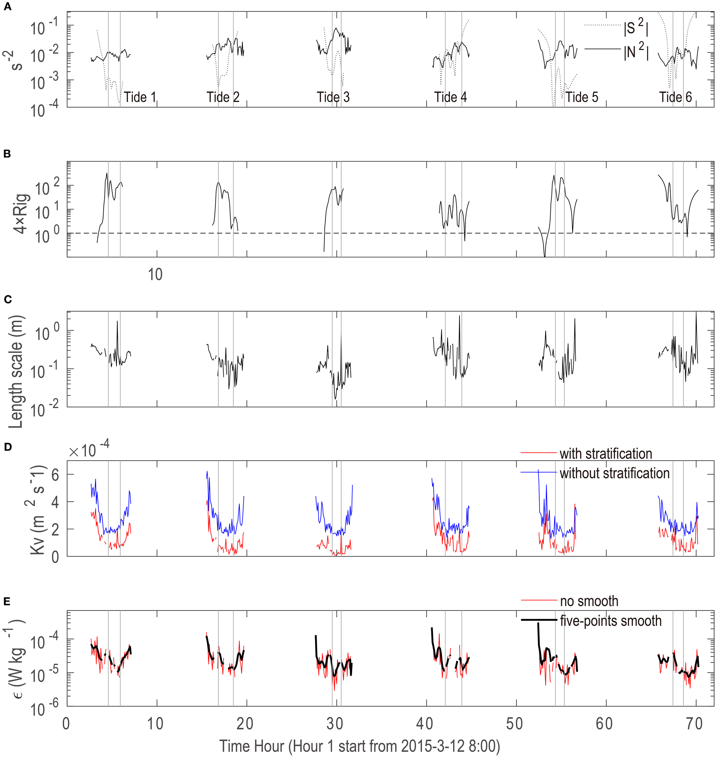
The temporal variation in turbulence parameters during observed tidal cycles. (A) The absolute values of squared velocity shear (|S2|) and the absolute values of buoyancy frequency (|N2|). (B) The gradient Richardson number (Rig). (C) The Ozmidov length scale (Lo). (D) Comparison between sediment eddy viscosity with (red line) and without stratification (blue line). (E) The turbulent kinetic energy dissipation rate (ϵ) with its five-point smooth value. The vertical gray lines show the periods of high SSC at high tide.
5.2.2 Local SSC balance in the near-bed layer
During high tide, the advection of SSC can be considered negligible, as both the horizontal velocity and horizontal gradient of SSC are significantly reduced. Consequently, the variation in near-bed SSC is primarily governed by the balance between sediment settling and vertical diffusion, as described by Equation 21:
where the first term represents the rate of SSC variation; the second term denotes the downward sediment flux induced by sediment settling, and the final term reflects the vertical diffusion of sediment due to turbulence. C is the sediment concentration, ws is the sediment settling velocity, and kc-str is the eddy diffusivity coefficient of suspended sediment induced by current influenced by sediment stratification. The vertical gradient of sediment concentration () is calculated as the difference between 0.1 mab and 0.3 mab
Based on Van Rijn (1993), the settling velocity is estimated as , where and D is the median sediment size. Assuming that the suspended sediment is mainly induced by the resuspension process, the median bed material size can be used to represent the median size of suspended sediment and has a value of 14 μm in this study. is the water kinematic viscosity and has a value of 1 × 10⁻⁶ m2 s-1. is the reduced gravity and is estimated as g(ρs-ρ0)/ρ0, where ρs is the density of sediment particles (2650 kg m-3) and ρ0 is the seawater density (1030 kg m-3). The settling velocity has a value of 1.68×10⁻⁴ m s-1.
Figure 10 compares the sediment settling flux and sediment diffusion flux. The temporal variation in sediment settling corresponds closely to the variation in SSC. Significant sediment settling occurs during flood and ebb surges, while it diminishes during high tide.
Figure 10
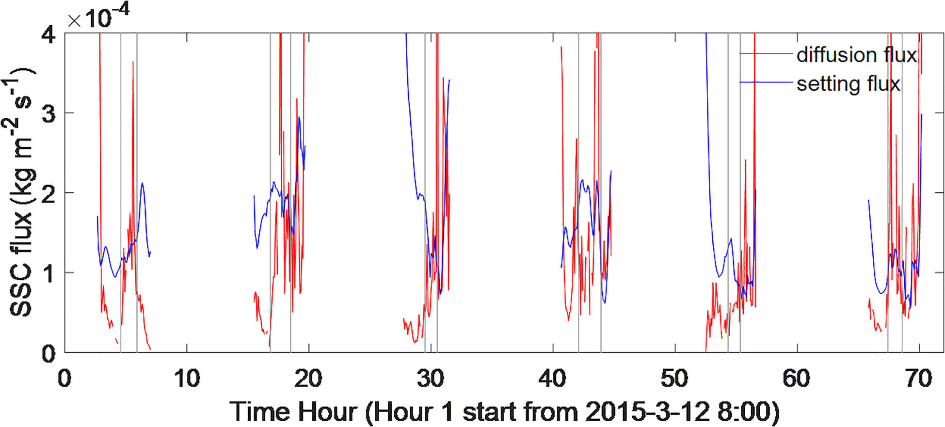
The balance of suspended sediment concentration in the near-bed layer, with sediment settling flux (blue line) and vertical sediment diffusion (red line), is depicted.
Intense near-bed stratification has a dual effect on sediment flux. On the one hand, stratification significantly reduces eddy diffusivity, thereby hindering upward sediment flux; on the other hand, severe stratification creates a steep sediment gradient, which enhances upward diffusion. When these two effects are combined, sediment vertical fluxes during high tide remain relatively substantial.
Positive vertical sediment diffusion is nearly balanced by downward sediment settling flux during high tide, particularly during tidal cycles 1, 3, and 6. This balance suggests that sediment from the upper layers is unable to settle below the 0.1 mab layer, indicating accumulation of sediment in the near-bed layer and the initiation of a near-bed high SSC event. During flood tides, the downward setting flux is generally larger than the upward sediment diffusion flux, which suggests that the sediment mainly sets downward.
The wave shear stress is significantly larger than the critical shear stress required for sediment suspension, indicating that sediment is resuspended mainly by waves from the seabed during high tide (Figure 8). Consequently, both sediment deposition from the upper layer and resuspended sediment from the seabed contribute to the formation of high near-bed SSC during high tide. In comparison, the current shear stress plays a minor role, as it is much smaller than the wave shear stress and is insufficient to suspend the sediment.
6 Conclusions
We conducted field observations to examine the temporal variation and vertical structure of sediment flux over an intertidal mudflat, characterized by significant tidal currents and surface waves. Tidal asymmetry is evident, with a shorter flood duration due to the generation of the M4 overtide in the shallow coastal ocean.
Tidal surges, associated with substantial bottom shear stress, occur regularly at the onset of flood tides and the end of ebb tides. Significant wave height and representative wave periods are substantial during high tide but diminish during tidal surges when the water is too shallow to allow large waves to propagate. The suspended sediment concentration (SSC) exhibits distinct temporal changes between the middle and near-bed layers. Peak SSC values above the middle layer are primarily induced by flood surges, followed by a continuous decrease. Ebb surges can occasionally suspend high sediment concentrations above the middle layer, but this is not consistent. In contrast, the near-bed SSC shows three peaks, corresponding to flood surges, ebb surges, and high tide.
Subtidal sediment flux demonstrates a two-layered structure, with landward flux occurring above the middle layer and seaward flux in the near-bed layer. A flood surge, carrying a high sediment concentration, promotes landward sediment transport above the middle layers. As the tidal current weakens, sediment from the upper layers begins to settle. During high tide, both upward diffusion due to tidal currents prevents further sediment settlement to the seabed, and large wave-induced bottom shear stress continually resuspend the sediment from seabed leading to accumulation of sediment in the near-bed layer. The high SSC at high tide largely coincides with the ebb current, which promotes seaward sediment transport. This study demonstrates that the combination of macrotides and significant wave activity creates favorable conditions for the two-layered subtidal sediment flux in intertidal mudflats. This two-layer sediment flux may not be unique to our study area, as similar patterns have been observed along the Jiangsu coast of China (Wang et al., 2012).
Our study investigates the pattern of sediment transport in intertidal mudflats under fair weather conditions. Tropical cyclones, including winter storms, typhoons, and hurricanes, can induce strong wind events. Under storm conditions, the two-layer structure of sediment flux may be significantly altered. Intense wave action during high tide leads to enhanced sediment suspension, while the strong winds may induce increased mixing, preventing the deposition of sediment from the upper layer. As a result, a more homogeneous vertical sediment profile may develop under storm conditions, potentially causing the attenuation or complete disruption of the two-layer sediment flux. A detailed analysis of sediment transport in intertidal mudflats under such conditions is warranted but falls beyond the scope of this study.
Statements
Data availability statement
The raw data supporting the conclusions of this article will be made available by the authors, without undue reservation.
Author contributions
QZ: Conceptualization, Formal Analysis, Writing – original draft. CW: Supervision, Methodology, Investigation, Writing – review & editing. WG: Formal Analysis, Writing – review & editing, Investigation. FZ: Funding acquisition, Supervision, Writing – review & editing.
Funding
The author(s) declare financial support was received for the research and/or publication of this article. This research was supported by the Open Research Fund of the State Key Laboratory of Estuarine and Coastal Research (Grant number SKLEC-KF202303), This work was financially supported by the National Natural Science Foundation of China (grant number 41906146; 41406101), the Key R&D Program of Zhejiang Province (grant number 2022C03044), the Zhejiang Provincial Ten Thousand Talents Plan (grant number 2020R52038), and the Zhejiang Provincial Project (grant number 330000210130313013006).
Acknowledgments
We thank our colleagues at the Zhejiang Institute of Hydraulics & Estuaries for carrying out the field measurements.
Conflict of interest
Author CW was employed by Shanghai Waterway Engineering Design and Consulting Co. Ltd.
The remaining authors declare that the research was conducted in the absence of any commercial or financial relationships that could be construed as a potential conflict of interest.
Generative AI statement
The author(s) declare that no Generative AI was used in the creation of this manuscript.
Any alternative text (alt text) provided alongside figures in this article has been generated by Frontiers with the support of artificial intelligence and reasonable efforts have been made to ensure accuracy, including review by the authors wherever possible. If you identify any issues, please contact us.
Publisher’s note
All claims expressed in this article are solely those of the authors and do not necessarily represent those of their affiliated organizations, or those of the publisher, the editors and the reviewers. Any product that may be evaluated in this article, or claim that may be made by its manufacturer, is not guaranteed or endorsed by the publisher.
References
1
Andersen T. J. Lanuru M. Van Bernem C. Pejrup M. Riethmueller R. (2010). Erodibility of a mixed mudflat dominated by microphytobenthos and Cerastoderma edule, East Frisian Wadden Sea, Germany. Estuarine Coast. Shelf Sci.87, 197–206. doi: 10.1016/j.ecss.2009.10.014
2
Aubrey D. G. Speer P. E. (1985). A study of non-linear tidal propagation in shallow inlet/estuarine systems Part I: Observations. Estuarine Coast. shelf Sci.21, 185–205. doi: 10.1016/0272-7714(85)90096-4
3
Bale A. J. Widdows J. Harris C. B. Stephens J. A. (2006). Measurements of the critical erosion threshold of surface sediments along the Tamar Estuary using a mini-annular flume. Continental Shelf Res.26, 1206–1216. doi: 10.1016/j.csr.2006.04.003
4
Barbier E. B. (2013). Valuing ecosystem services for coastal wetland protection and restoration: Progress and challenges. Resources2, 213–230. doi: 10.3390/resources2030213
5
Bassoullet P. Le Hir P. Gouleau D. Robert S. (2000). Sediment transport over an intertidal mudflat: field investigations and estimation of fluxes within the “Baie de Marenngres-Oleron”(France). Continental shelf Res.20, 1635–1653. doi: 10.1016/S0278-4343(00)00041-8
6
Bendat J. S. Piersol A. G. (2000). Random data analysis and measurement procedures. Measurement Sci. Technol.11, 1825–1826. doi: 10.1088/0957-0233/11/12/702
7
Benilov A. Y. Filyushkin B. N. (1970). Application of methods of linear filtration to an analysis of fluctuations in the surface layer of the sea. Izv. Acad. Sci. USSR Atmos. Oceanic Phys.68, 810–819.
8
Bian C. Liu Z. Huang Y. Zhao L. Jiang W. (2018). On estimating turbulent Reynolds stress in wavy aquatic environment. J. Geophysical Research: Oceans123, 3060–3071. doi: 10.1002/2017JC013230
9
Bian C. Liu X. Zhou Z. Chen Z. Wang T. Gu Y. (2020). Calculation of winds induced bottom wave orbital velocity using the empirical mode decomposition method. J. Atmospheric Oceanic Technol.37, 889–900. doi: 10.1175/JTECH-D-19-0185.1
10
Bluteau C. E. Jones N. L. Ivey G. N. (2011). Estimating turbulent kinetic energy dissipation using the inertial subrange method in environmental flows. Limnology Oceanography: Methods9, 302–321. doi: 10.4319/lom.2011.9.302
11
Bricker J. D. Monismith S. G. (2007). Spectral wave–turbulence decomposition. J. Atmospheric Oceanic Technol.24, 1479–1487. doi: 10.1175/JTECH2066.1
12
Chen X. Santos I. R. Hu D. Zhan L. Zhang Y. Zhao Z. et al . (2022). Pore-water exchange flushes blue carbon from intertidal saltmarsh sediments into the sea. Limnology oceanography Lett.7, 312–320. doi: 10.1002/lol2.10236
13
Christie M. C. Dyer K. R. Turner P. (1999). Sediment flux and bed level measurements from a macro tidal mudflat. Estuarine Coast. Shelf Sci.49, 667–688. doi: 10.1006/ecss.1999.0525
14
Chung C. H. Zhuo R. Z. Xu G. W. (2004). Creation of Spartina plantations for reclaiming Dongtai, China, tidal flats and offshore sands. Ecol. Eng.23, 135–150. doi: 10.1016/j.ecoleng.2004.07.004
15
Cook P. L. Butler E. C. Eyre B. D. (2004a). Carbon and nitrogen cycling on intertidal mudflats of a temperate Australian estuary. I. Benthic metabolism. Mar. Ecol. Prog. Ser.280, 25–38. doi: 10.3354/meps280025
16
Cook P. L. Revill A. T. Butler E. C. Eyre B. D. (2004b). Carbon and nitrogen cycling on intertidal mudflats of a temperate Australian estuary. II. Nitrogen cycling. Mar. Ecol. Prog. Ser.280, 39–54. doi: 10.3354/meps280039
17
Costanza R. Pérez-Maqueo O. Martinez M. L. Sutton P. Anderson S. J. Mulder K. (2008). The value of coastal wetlands for hurricane protection. Ambio. 37, 241–248. doi: 10.1579/0044-7447(2008)37[241:TVOCWF]2.0.CO;2
18
Dyer K. R. Christie M. C. Feates N. Fennessy M. J. Pejrup M. Van der Lee W. (2000). An investigation into processes influencing the morphodynamics of an intertidal mudflat, the Dollard Estuary, the Netherlands: I. Hydrodynamics and suspended sediment. Estuarine Coast. Shelf Sci.50, 607–625. doi: 10.1006/ecss.1999.0596
19
Feddersen F. Guza R. T. (2003). Observations of nearshore circulation: Alongshore uniformity. J. Geophysical Research: Oceans108, 6–1. doi: 10.1029/2001JC001293
20
Feddersen F. Williams III, A. J. (2007). Direct estimation of the Reynolds stress vertical structure in the nearshore. J. Atmospheric Oceanic Technol.24, 102–116. doi: 10.1175/JTECH1953.1
21
Feng X. Tsimplis M. N. (2014). Sea level extremes at the coasts of China. J. Geophysical Research: Oceans119, 1593–1608. doi: 10.1002/2013JC009607
22
Foster N. M. Hudson M. D. Bray S. Nicholls R. J. (2013). Intertidal mudflat and saltmarsh conservation and sustainable use in the UK: A review. J. Environ. Manage.126, 96–104. doi: 10.1016/j.jenvman.2013.04.015
23
French C. E. French J. R. Clifford N. J. Watson C. J. (2000). Sedimentation–erosion dynamics of abandoned reclamations: the role of waves and tides. Continental Shelf Res.20, 1711–1733. doi: 10.1016/S0278-4343(00)00044-3
24
Friedrichs C. T. Aubrey D. G. (1988). Non-linear tidal distortion in shallow well-mixed estuaries: a synthesis. Estuarine Coast. Shelf Sci.27, 521–545. doi: 10.1016/0272-7714(88)90082-0
25
Gao J. Hou L. Liu Y. Shi H. (2024). Influences of bragg reflection on harbor resonance triggered by irregular wave groups. Ocean Eng.305, 117941. doi: 10.1016/j.oceaneng.2024.117941
26
Gedan K. B. Kirwan M. L. Wolanski E. Barbier E. B. Silliman B. R. (2011). The present and future role of coastal wetland vegetation in protecting shorelines: answering recent challenges to the paradigm. Climatic Change106, 7–29. doi: 10.1007/s10584-010-0003-7
27
Glenn S. M. Grant W. D. (1987). A suspended sediment stratification correction for combined wave and current flows. J. Geophysical Research: Oceans92, 8244–8264. doi: 10.1029/JC092iC08p08244
28
Govers G. (1987). Initiation of motion in overland flow. Sedimentology34, 1157–1164. doi: 10.1111/j.1365-3091.1987.tb00598.x
29
Grant W. D. Madsen O. S. (1979). Combined wave and current interaction with a rough bottom. J. Geophysical Research: Oceans84, 1797–1808. doi: 10.1029/JC084iC04p01797
30
Grant W. D. Madsen O. S. (1986). The continental-shelf bottom boundary layer. Annual Review of Fluid Mechanics18 (1), 265–305. doi: 10.1146/annurev.fl.18.010186.001405
31
Green M. O. Black K. P. Amos C. L. (1997). Control of estuarine sediment dynamics by interactions between currents and waves at several scales. Mar. geology144, 97–116. doi: 10.1016/S0025-3227(97)00065-0
32
Huntley D. A. Hazen D. G. (1988). Seabed stresses in combined wave and steady flow conditions on the Nova Scotia continental shelf: Field measurements and predictions. J. Phys. Oceanography18, 347–362. doi: 10.1175/1520-0485(1988)018<0347:SSICWA>2.0.CO;2
33
Janssen-Stelder B. (2000). The effect of different hydrodynamic conditions on the morphodynamics of a tidal mudflat in the Dutch Wadden Sea. Continental shelf Res.20, 1461–1478. doi: 10.1016/S0278-4343(00)00032-7
34
Jensen B. L. Sumer B. M. Fredsøe J. (1989). Turbulent oscillatory boundary layers at high Reynolds numbers. J. Fluid Mechanics206, 265–297. doi: 10.1017/S0022112089002302
35
Keen T. R. Glenn S. M. (2002). Predicting bed scour on the continental shelf during Hurricane Andrew. J. waterway port coastal ocean Eng.128, 249–257. doi: 10.1061/(ASCE)0733-950X(2002)128:6(249)
36
Kim S. C. Friedrichs C. T. Maa J. Y. Wright L. D. (2000). Estimating bottom stress in tidal boundary layer from acoustic Doppler velocimeter data. J. Hydraulic Eng.126, 399–406. doi: 10.1061/(ASCE)0733-9429(2000)126:6(399)
37
Kolmogorov A. N. (1941). “The local structure of turbulence in incompressible viscous fluids for very large Reynolds numbers,” in Doklady Akademii Nauk SSSR, 30. p. 301–305.
38
Le Hir P. Roberts W. Cazaillet O. Christie M. Bassoullet P. Bacher C. (2000). Characterization of intertidal flat hydrodynamics. Continental shelf Res.20, 1433–1459. doi: 10.1016/S0278-4343(00)00031-5
39
Lesieur M. Comte P. Lamballais E. Métais O. Silvestrini G. (1997). Large-eddy simulations of shear flows. J. Eng. Mathematics32, 195–215. doi: 10.1023/A:1004228831518
40
Liu Z. Wei H. (2007). Estimation to the turbulent kinetic energy dissipation rate and bottom shear stress in the tidal bottom boundary layer of the Yellow Sea. Prog. Natural Sci.17, 289–297. doi: 10.1080/10020070612331343260
41
Longuet-Higgens M. S. (1952). On the statistical distribution of the heights of sea waves. J. Mar. Res.11, 245–266.
42
Lozovatsky I. Liu Z. Wei H. Fernando H. J. S. (2008). Tides and mixing in the northwestern East China Sea, Part II: Near-bottom turbulence. Continental Shelf Res.28, 338–350. doi: 10.1016/j.csr.2007.08.007
43
MacVean L. J. Lacy J. R. (2014). Interactions between waves, sediment, and turbulence on a shallow estuarine mudflat. J. Geophysical Research: Oceans119, 1534–1553. doi: 10.1002/2013JC009477
44
Mantz P. A. (1977). Incipient transport of fine grains and flakes by fluids—extended Shields diagram. J. Hydraulics division103, 601–615. doi: 10.1061/JYCEAJ.0004766
45
Möller I. Kudella M. Rupprecht F. Spencer T. Paul M. Van Wesenbeeck B. K. et al . (2014). Wave attenuation over coastal salt marshes under storm surge conditions. Nat. Geosci.7, 727–731. doi: 10.1038/ngeo2251
46
Pawlowicz R. Beardsley B. Lentz S. (2002). Classical tidal harmonic analysis including error estimates in MATLAB using T_TIDE. Comput. Geosciences28, 929–937. doi: 10.1016/S0098-3004(02)00013-4
47
Postma H. E. N. D. R. I. K. (1961). Transport and accumulation of suspended matter in the Dutch Wadden Sea. Netherlands J. Sea Res.1, 148–190. doi: 10.1016/0077-7579(61)90004-7
48
Qiao F. Yuan Y. Deng J. Dai D. Song Z. (2016). Wave–turbulence interaction-induced vertical mixing and its effects in ocean and climate models. Philos. Trans. R. Soc. A: Mathematical Phys. Eng. Sci.374, 20150201. doi: 10.1098/rsta.2015.0201
49
Ralston D. K. Stacey M. T. (2007). Tidal and meteorological forcing of sediment transport in tributary mudflat channels. Continental Shelf Res.27, 1510–1527. doi: 10.1016/j.csr.2007.01.010
50
Riley J. J. Lindborg E. (2008). Stratified turbulence: A possible interpretation of some geophysical turbulence measurements. J. Atmospheric Sci.65, 2416–2424. doi: 10.1175/2007JAS2455.1
51
Sanford L. P. (1994). Wave-forced resuspension of upper Chesapeake Bay muds. Estuaries17, 148–165. doi: 10.2307/1352564
52
Shaw W. J. Trowbridge J. H. (2001). The direct estimation of near-bottom turbulent fluxes in the presence of energetic wave motions. J. Atmospheric oceanic Technol.18, 1540–1557. doi: 10.1175/1520-0426(2001)018<1540:TDEONB>2.0.CO;2
53
Shi B. Cooper J. R. Li J. Yang Y. Yang S. L. Luo F. et al . (2019). Hydrodynamics, erosion and accretion of intertidal mudflats in extremely shallow waters. J. Hydrology573, 31–39. doi: 10.1016/j.jhydrol.2019.03.065
54
Shi B. Cooper J. R. Pratolongo P. D. Gao S. Bouma T. J. Li G. et al . (2017). Erosion and accretion on a mudflat: the importance of very shallow-water effects. J. Geophysical Research: Oceans122, 9476–9499. doi: 10.1002/2016JC012316
55
Shi B. W. Yang S. L. Wang Y. P. Bouma T. J. Zhu Q. (2012). Relating accretion and erosion at an exposed tidal wetland to the bottom shear stress of combined current–wave action. Geomorphology138, 380–389. doi: 10.1016/j.geomorph.2011.10.004
56
Shi B. W. Yang S. L. Wang Y. P. Yu Q. Li M. L. (2014). Intratidal erosion and deposition rates inferred from field observations of hydrodynamic and sedimentary processes: A case study of a mudflat–saltmarsh transition at the Yangtze delta front. Continental Shelf Res.90, 109–116. doi: 10.1016/j.csr.2014.01.019
57
Soulsby R. L. (1995). “Bed shear stresses due to combined waves and currents.” In StiveM. J. F.De VriendH. J.FredseJ.HammL.SoulsbyR. L.TeissonC.et al (Eds.), Advances in Coastal Morphodynamics: An Overview of the G-8 Coastal Morphodynamics Project. Delft, The Netherlands: Delft Hydraulics. pp. 420–423.
58
Sreenivasan K. R. Kailasnath P. (1993). An update on the intermittency exponent in turbulence. Phys. Fluids A: Fluid Dynamics5, 512–514. doi: 10.1063/1.858877
59
Stapleton K. R. Huntley D. A. (1995). Seabed stress determinations using the inertial dissipation method and the turbulent kinetic energy method. Earth surface processes landforms20, 807–815. doi: 10.1002/esp.3290200906
60
Straaten L. V. Kuenen P. H. (1958). Tidal action as a cause of clay accumulation. J. Sedimentary Res.28, 406–413. doi: 10.1306/74D70826-2B21-11D7-8648000102C1865D
61
Styles R. Glenn S. M. (2002). Modeling bottom roughness in the presence of wave-generated ripples. J. Geophysical Research: Oceans107, 24–21. doi: 10.1029/2001JC000864
62
Taki K. (2000). “Critical shear stress for cohesive sediment transport,” in Proceedings in Marine Science, vol. 3. (Amsterdam: Elsevier), 53–61.
63
Talke S. A. Stacey M. T. (2008). Suspended sediment fluxes at an intertidal flat: the shifting influence of wave, wind, tidal, and freshwater forcing. Continental Shelf Res.28, 710–725. doi: 10.1016/j.csr.2007.12.003
64
Temmerman S. De Vries M. B. Bouma T. J. (2012). Coastal marsh die-off and reduced attenuation of coastal floods: A model analysis. Global Planetary Change92, 267–274. doi: 10.1016/j.gloplacha.2012.06.001
65
Trowbridge J. H. (1998). On a technique for measurement of turbulent shear stress in the presence of surface waves. J. Atmospheric Oceanic Technol.15, 290–298. doi: 10.1175/1520-0426(1998)015<0290:OATFMO>2.0.CO;2
66
Van Rijn L. C. Nieuwjaar M. W. van der Kaay T. Nap E. van Kampen A. (1993). Transport of fine sands by currents and waves. J. waterway port coastal ocean Eng.119, 123–143. doi: 10.1061/(ASCE)0733-950X(1993)119:2(123)
67
Wang Y. Gao S. Jia J. (2006). High-resolution data collection for analysis of sediment dynamic processes associated with combined current-wave action over intertidal flats. Chin. Sci. Bull.51, 866–877. doi: 10.1007/s11434-006-0866-1
68
Wang Y. P. Gao S. Jia J. Thompson C. E. Gao J. Yang Y. (2012). Sediment transport over an accretional intertidal flat with influences of reclamation, Jiangsu coast, China. Mar. Geology291, 147–161. doi: 10.1016/j.margeo.2011.01.004
69
Wang X. Ke X. (1997). Grain-size characteristics of the extant tidal flat sediments along the Jiangsu coast, China. Sedimentary Geology112, 105–122. doi: 10.1016/S0037-0738(97)00026-2
70
Wang Y. P. Voulgaris G. Li Y. Yang Y. Gao J. Chen J. et al . (2013). Sediment resuspension, flocculation, and settling in a macrotidal estuary. J. Geophysical Research: Oceans118, 5591–5608. doi: 10.1002/jgrc.20340
71
Wiberg P. L. Sherwood C. R. (2008). Calculating wave-generated bottom orbital velocities from surface-wave parameters. Comput. Geosciences34, 1243–1262. doi: 10.1016/j.cageo.2008.02.010
72
Xing F. Wang Y. P. Wang H. V. (2012). Tidal hydrodynamics and fine-grained sediment transport on the radial sand ridge system in the southern Yellow Sea. Mar. geology291, 192–210. doi: 10.1016/j.margeo.2011.06.006
73
Yang S. L. Friedrichs C. T. Shi Z. Ding P. X. Zhu J. Zhao Q. Y. (2003). Morphological response of tidal marshes, flats and channels of the outer Yangtze River mouth to a major storm. Estuaries26, 1416–1425. doi: 10.1007/BF02803650
74
Ye Q. Yang Z. Bao M. Shi W. Shi H. You Z. et al . (2022). Distribution characteristics of wave energy in the Zhe-Min coastal area. Acta Oceanologica Sin.41, 163–172. doi: 10.1007/s13131-021-1859-2
75
Ysebaert T. Herman P. M. J. Meire P. Craeymeersch J. Verbeek H. Heip C. H. R. (2003). Large-scale spatial patterns in estuaries: estuarine macrobenthic communities in the Schelde estuary, NW Europe. Estuarine Coast. shelf Sci.57, 335–355. doi: 10.1016/S0272-7714(02)00359-1
76
Yuan Y. Wei H. Zhao L. Jiang W. (2008). Observations of sediment resuspension and settling off the mouth of Jiaozhou Bay, Yellow Sea. Continental Shelf Res.28, 2630–2643. doi: 10.1016/j.csr.2008.08.005
77
Zhang Q. Gong Z. Zhang C. Lacy J. Jaffe B. Xu B. et al . (2021). The role of surges during periods of very shallow water on sediment transport over tidal flats. Front. Mar. Sci.8, 599799. doi: 10.3389/fmars.2021.599799
78
Zhang Q. Gong Z. Zhang C. Townend I. Jin C. Li H. (2016). Velocity and sediment surge: What do we see at times of very shallow water on intertidal mudflats? Continental Shelf Res.113, 10–20. doi: 10.1016/j.csr.2015.12.003
79
Zhu S. Wei W. Zhu Q. Wan K. Xing F. Yan W. et al . (2024). Wave attenuation and transformation across a highly turbid muddy tidal flat-salt marsh system. Appl. Ocean Res.147, 103980. doi: 10.1016/j.apor.2024.103980
Summary
Keywords
sediment transport, intertidal mudflat, surface wave, high sediment concentration, tidal currents, turbulence
Citation
Zhang Q, Wu C, Gu W and Zhou F (2025) Two-layered structure of subtidal sediment flux across intertidal mudflats due to tidal surges and surface waves. Front. Mar. Sci. 12:1667003. doi: 10.3389/fmars.2025.1667003
Received
16 July 2025
Accepted
27 August 2025
Published
17 September 2025
Volume
12 - 2025
Edited by
Dongfeng Xie, Zhejiang Institute of Hydraulics & Estuary, China
Reviewed by
Junliang Gao, Jiangsu University of Science and Technology, China
Shenliang Chen, East China Normal University, China
Updates
Copyright
© 2025 Zhang, Wu, Gu and Zhou.
This is an open-access article distributed under the terms of the Creative Commons Attribution License (CC BY). The use, distribution or reproduction in other forums is permitted, provided the original author(s) and the copyright owner(s) are credited and that the original publication in this journal is cited, in accordance with accepted academic practice. No use, distribution or reproduction is permitted which does not comply with these terms.
*Correspondence: Feng Zhou, zhoufeng@sio.org.cn
Disclaimer
All claims expressed in this article are solely those of the authors and do not necessarily represent those of their affiliated organizations, or those of the publisher, the editors and the reviewers. Any product that may be evaluated in this article or claim that may be made by its manufacturer is not guaranteed or endorsed by the publisher.