Abstract
Mesoscale eddies exert profound influences on marine environments, thereby regulating habitat quality and the distribution of marine organisms. The waters off Chile are a region of intense mesoscale eddy activity and represent a major habitat for the jumbo flying squid (Dosidicus gigas), a short-lived and economically important species. However, the effects of mesoscale eddies on the habitat of D. gigas in this region remain poorly understood. In this study, we integrated autumn (March-May) fisheries data of D. gigas from 2015 to 2021 with environmental variables, including sea surface temperature (SST), chlorophyll-a concentration (Chl-a), and sea surface dissolved oxygen concentration (DO), to develop and validate habitat suitability index (HSI) models with different weighting schemes. Using the optimal HSI model in combination with mesoscale eddy data, we compared the impacts of cyclonic and anticyclonic eddies on D. gigas abundance and habitat suitability. The results revealed that the optimal HSI model effectively predicted the potential habitats of D. gigas, with weights for SIDO, SISST, and SIChl-a of 0.1, 0.1, and 0.8, respectively. Compared with anticyclonic eddies, cyclonic eddies provided broader areas of suitable habitats, characterized by suitable Chl-a and DO levels, and supported higher D. gigas abundances. Furthermore, the habitat suitability of D. gigas within mesoscale eddies exhibited interannual variability and was significantly correlated with the radius, velocity, and amplitude of the eddies. This study highlighted the critical role of mesoscale eddies in shaping the habitat suitability of D. gigas and provided valuable insights for the management and conservation of cephalopod resources.
1 Introduction
A habitat refers to the environment on which organisms depend for survival, growth, and reproduction (National Research Council, 1982). Different species have specific habitat requirements, and changes in habitat conditions can directly affect population dynamics. Therefore, analyzing and assessing habitat quality is essential for the conservation and management of biological populations. The habitat suitability index (HSI) model is a widely used approach to evaluate habitat quality and assess potential developmental impacts (Hightower et al., 2012). First proposed in the 1980s by the U.S. Geological Survey National Wetlands Research Center and Fish and Wildlife Department (Yu et al., 2015), the HSI model is valued for its simplicity, ease of interpretation, and robust performance. Its outputs can be integrated with geographic information systems (GIS), providing managers with practical decision-making tools (Vinagre et al., 2006). Today, HSI models have been extensively applied in evaluating habitats and predicting fishing grounds for marine cephalopods and fish species (Chen et al., 2009; Li et al., 2014; Tian et al., 2009). For instance, Wen et al. (2025) utilized an HSI model to analyze the effects of Indian Ocean Dipole (IOD) events on the habitat of Sthenoteuthis oualaniensis, revealing that negative IOD events resulted in more extensive suitable habitats compared to positive IOD phases.
The ocean encompasses dynamic processes across multiple spatial and temporal scales, among which mesoscale processes (approximately 50–500 km) represent a critical component (Covington et al., 2025), typically arising from oceanic instabilities (McGillicuddy, 2016). Mesoscale eddies, a key manifestation of these dynamics, are pervasive rotational structures that dominate the oceanic environment, accounting for a substantial portion of the ocean’s total kinetic energy (Chelton et al., 2011; Wunsch and Ferrari, 2004). Generally, mesoscale eddies are classified into two types: cyclonic eddies (CEs), characterized by cooler water in their cores compared to the surrounding sea and thus referred to as cold eddies, and anticyclonic eddies (AEs), marked by warmer core waters and commonly termed warm eddies (Bakun, 2006). These eddies redistribute salinity, heat, and other substances, influencing general circulation, underwater sound propagation, and even the ocean’s capacity for carbon dioxide absorption (Chelton et al., 2007; Li et al., 2025; Zhang et al., 2025). Moreover, they play significant roles in wind, clouds, rainfall, and marine heatwaves (Bian et al., 2023; Frenger et al., 2013; Ma et al., 2015). Importantly, mesoscale eddies are also recognized as critical drivers of habitat quality and the spatial distribution of marine organisms. For example, Davis et al. (2002) reported that CEs in the northern Gulf of Mexico serve as preferred foraging areas for cetaceans due to the aggregation of abundant prey, while Nieto et al. (2014) found that mesoscale eddies in the southern Gulf of California entrain suitable water masses, thereby creating suitable spawning habitats for sardines. These findings highlight the necessity of elucidating the influence and underlying mechanisms of mesoscale eddies on the habitats of diverse marine species to support sustainable fisheries management.
The jumbo flying squid (Dosidicus gigas), belonging to the family Ommastrephidae, is a highly valuable economic species widely distributed east of 140°W (Chen et al., 2008). Compared to other members of Ommastrephidae, D. gigas is characterized by its large body size, thick flesh, rapid juvenile growth, and strong predatory capacity (Ibáñez et al., 2016; Nigmatullin, 2001). Notably, its population structure, dietary composition, and migratory patterns exhibit variation across different geographic regions (Ibáñez et al., 2016; Nigmatullin, 2001). The waters off Chile harbor abundant D. gigas resources; as early as the 1960s, Soviet fishing vessels reported massive aggregations of the species in these coastal areas (Yu et al., 2025). Today, this region remains one of the world’s primary fishing grounds for D. gigas. Known for its high sensitivity to environmental variability, even minor changes in oceanographic conditions can lead to significant shifts in its habitat distribution (Yu et al., 2025). Feng et al. (2025) found that when sea surface height above geoid anomaly decreased and sea surface salinity and 400 m water layer temperature increased, the area of suitable habitat for D. gigas increased. The Chilean waters, situated within a boundary upwelling system, are an area with active mesoscale eddy activity (Chaigneau et al., 2009). Although previous studies have demonstrated the significant influence of mesoscale eddies on the habitat distribution of Ommastrephidae species (Alabia et al., 2015; Della Penna et al., 2022), research on how eddies affect the habitat of D. gigas in the Chilean region remains remarkably scarce.
To this end, this study developed an HSI model using D. gigas fisheries data and oceanographic environmental data from the waters off Chile and integrated mesoscale eddy datasets to analyze differences in the abundance and habitat distribution of D. gigas within CEs and AEs. The findings aim to provide a scientific basis for the conservation and sustainable utilization of D. gigas resources.
2 Materials and methods
2.1 Fisheries, environmental and mesoscale eddy data
From March to May during 2015-2021, D. gigas fisheries data were obtained from the National Distant-water Fisheries Data Center of China (NDFDC), Shanghai Ocean University, China. The fishing activities were conducted in the southeastern Pacific Ocean, covering the area between 70°-97°W and 20°-47°S. The dataset included information on fishing locations (longitude and latitude), fishing dates (year, month, day), catch (tons), and fishing effort (days). Catch per unit effort (CPUE, in unit of: t/d), calculated as the ratio of catch to fishing effort, was used as an indicator of D. gigas abundance.
A previous study (Wu et al., 2025) has shown that among the ten environmental factors, including sea surface height, sea surface salinity, and others, sea surface temperature (SST), chlorophyll-a concentration (Chl-a), and sea surface dissolved oxygen concentration (DO) are the environmental factors that have a significant impact on D. gigas. Consequently, this study focused on SST, Chl-a, and DO for subsequent analysis. SST data were obtained from the global ocean physics reanalysis product provided by the Copernicus Marine Environment Monitoring Service (CMEMS) (https://data.marine.copernicus.eu/product/GLOBAL_MULTIYEAR_PHY_001_030/description), with a daily temporal resolution and a spatial resolution of 0.083°. Chl-a and DO data were sourced from the CMEMS global ocean biogeochemical hindcast product (https://data.marine.copernicus.eu/product/GLOBAL_MULTIYEAR_BGC_001_029/description), with a daily temporal resolution and a spatial resolution of 0.25°. The environmental datasets fully covered the spatial extent of the study area and were matched with the fisheries data for subsequent analyses.
The mesoscale eddy dataset used in this study was obtained from the eddy trajectory atlas product (META ver3.2), produced by SSALTO/DUACS and distributed by AVISO+ (https://aviso.altimetry.fr). This dataset identifies eddies based on absolute dynamic topography data with a spatial resolution of 0.25°, providing a more accurate representation of ocean dynamics in coastal regions, around islands, and in highly energetic areas (Pegliasco et al., 2022). We utilized the all-satellite version of this dataset, which includes daily information from January 2015 to December 2021 on the lifecycles, radius (unit: km), eddy center positions, velocity (unit: m/s), boundary contours, and amplitudes (unit: m) of CEs and AEs within the study area. Figure 1 showed the spatial distribution of eddies in the study area on March 1, 2016.
Figure 1
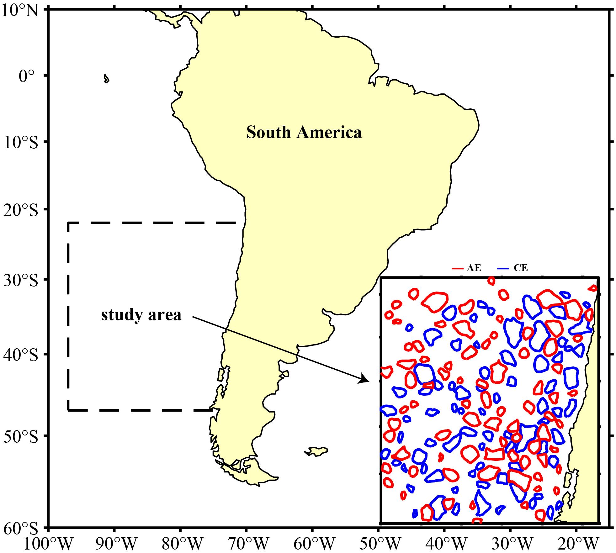
Spatial distribution of cyclonic and anticyclonic eddies on March 1, 2016 within the study area (blue lines were cyclonic eddies, red lines were anticyclonic eddies, and yellow areas were land).
2.2 Construction and validation of HSI model
This study incorporated fishing effort, SST, Chl-a, and DO into the HSI model. The process of constructing and validating the HSI model was as follows:
(1) Construction of the suitability index (SI) model. The observed SI was derived by calculating the ratio of fishing effort within a specific environmental variable classification interval to the maximum fishing effort within that interval (Yu et al., 2015). Based on previous studies and further testing (Feng et al., 2022, 2025; Jin et al., 2024a), the classification interval of SST was set to 0.5 °C for March, April, and May; that of Chl-a was 0.02, 0.03, and 0.02 mg/m³, respectively; and that of DO was 4, 2, and 3 mmol/m³, respectively. The observed SI values and classification intervals of each environmental variable were then used as input parameters to construct the fitted SI model according to the following equation (Wen et al., 2025):
where and were model parameters to be estimated; was the classification interval values for each environmental variable.
(2) Assignment of model weights. Different weights (Supplementary Table S1) were assigned to the SI models of each environmental variable and then combined to construct the HSI model. The HSI model was calculated using the following equation:
where was the weight assigned to environmental variable ; was the total number of environmental variables included in the HSI model.
(3) Selection of the optimal model (a suboptimal solution within a limited parameter space). HSI values ranged from 0 to 1. Regions with HSI ≤ 0.2, 0.2 < HSI < 0.6, and HSI ≥ 0.6 were classified as poor, moderate, and suitable habitats, respectively (Feng et al., 2022). Typically, in suitable habitats, the proportions of catch and fishing effort relative to their totals were greater, whereas the opposite trend was observed in poor habitats. Furthermore, as HSI increased, the proportions of catch and fishing effort also increased (Yu et al., 2015). Based on this theory, the optimal model was selected.
(4) Model validation. The HSI model was constructed using D. gigas fisheries and environmental data from 2015 to 2018. Habitat suitability for 2019–2021 was predicted and compared to actual D. gigas fisheries data to assess the model’s performance.
2.3 Analysis of differences in the distribution of D.gigas habitat within CEs and AEs
This study defined the eddy influence range as twice its actual coverage area (Zhou et al., 2021). Given that eddies often exhibit irregular shapes, a standardized circular grid was applied to uniformly represent the daily influence range of each eddy. The radius of this standardized circular grid was 2R, where R was the radius of the circle that best approximates the shape of the eddy’s outermost closed contour (Pegliasco et al., 2022). This circular grid was further divided into two regions: the 0-R region, which was the inner circle from the center to R, and the R-2R region, which was the annular zone extending from R to 2R. Using daily D. gigas fishing location data and eddy boundary contours data, grids containing D. gigas fishing points were identified for each day, and the CPUE of D. gigas within grids of different eddy types was calculated. A t-test was then employed to compare the CPUE differences between CEs and AEs.
Based on the optimal HSI model described in Section 2.2, daily D. gigas HSI values were computed across the study area. The HSI values corresponding to circular eddy grids containing D. gigas fishing points were extracted, grouped by eddy polarity and year, and averaged to compare habitat quality between the two eddy types and to assess interannual variation. Furthermore, the study examined how the proportion of suitable habitat area within circular eddy grids varied with increasing distance from the eddy center.
2.4 Influence of eddy parameters on habitat suitability for D.gigas
This study employed a generalized additive model (GAM) to analyze the effects of eddy parameters on the habitat suitability of D. gigas within their influence ranges. The GAM, a nonparametric extension of the generalized linear model, was capable of describing nonlinear relationships between response and explanatory variables (Han et al., 2022). The GAM was constructed as follows:
where was the mean HSI of D. gigas within CEs or AEs; was the link function; was the intercept; was the smooth function; was eddy parameters (radius, velocity, and amplitude); was the random error.
Prior to GAM analysis, variance inflation factors (VIF) were calculated to test for multicollinearity among explanatory variables. The results indicated no significant multicollinearity (VIF < 10) (O’brien, 2007). The GAM analyses were conducted in R (Version 4.4.0) using the “mgcv” (Version 1.9-1) package.
3 Results
3.1 HSI model results
The SI curves for SST, Chl-a, and DO, fitted using over 2000 D. gigas fishing points data collected from March to May 2015–2018 off Chile, were shown in Figure 2, and the corresponding SI model parameters were summarized in Table 1. All SI models were highly significant and demonstrated strong fits (R² > 0.8, P < 0.001). The fitted SI curves exhibited clear normal distributions and closely matched the observed SI values. The suitable environmental ranges within the D. gigas fishing grounds off Chile were approximately: March (SST: 19.59-20.37 °C; Chl-a: 0.13-0.16 mg/m³; DO: 230.02-233.55 mmol/m³), April (SST: 19.45-20.59 °C; Chl-a: 0.12-0.14 mg/m³; DO: 228.58-231.39 mmol/m³), and May (SST: 19.20-20.80 °C; Chl-a: 0.12-0.14 mg/m³; DO: 227.13-236.04 mmol/m³).
Figure 2
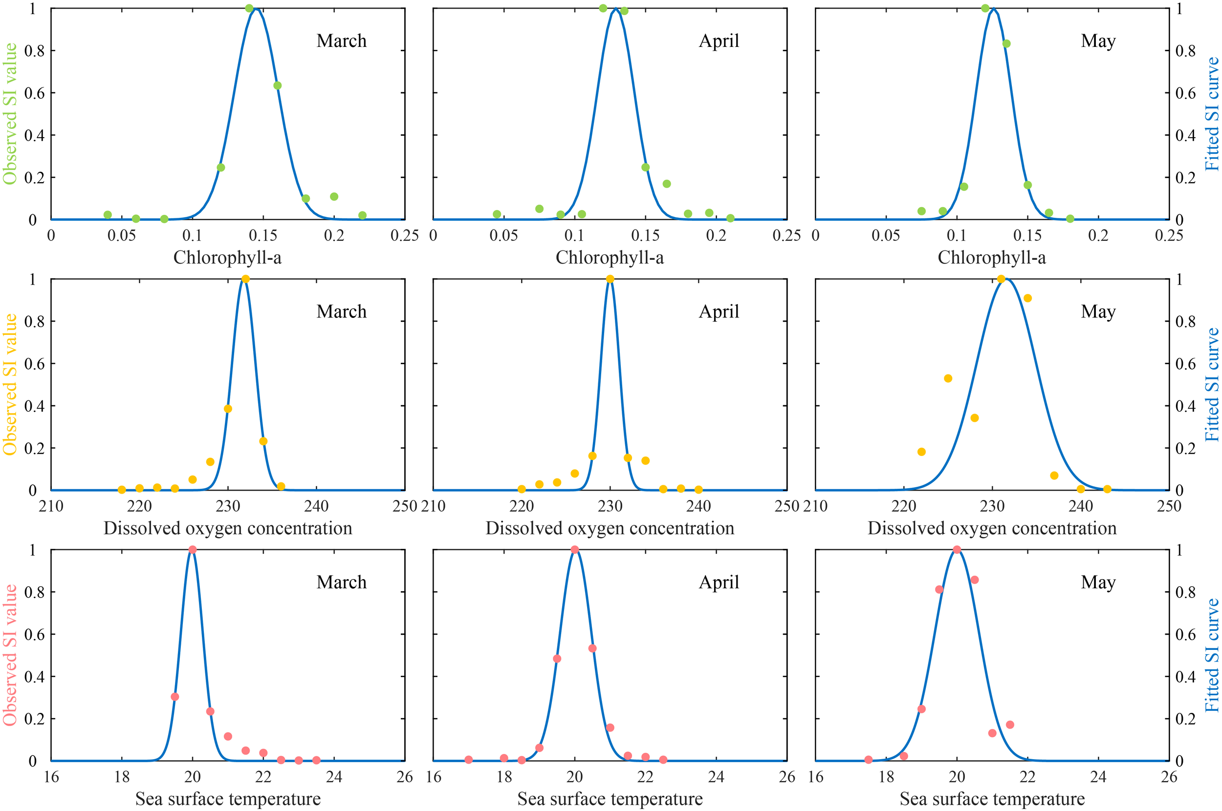
Suitability index (SI) curves inferred from the relationship between fishing effort and sea surface temperature (SST), chlorophyll-a concentration (Chl-a) and dissolved oxygen concentration (DO) from March to May (dot: observed SI value; blue solid line: fitted SI value).
Table 1
| Month | SI model for each environmental variable | R2 | P |
|---|---|---|---|
| March | SIChl-a=exp[-2071.857(XChl-a-0.145)2] SIDO=exp[-0.289(XDO-231.784)2] SISST=exp[-5.214(XSST-19.977)2] |
0.984 | <0.001 |
| 0.98 | <0.001 | ||
| 0.98 | <0.001 | ||
| April | SIChl-a=exp[-2945.822(XChl-a-0.129)2] SIDO=exp[-0.459(XDO-229.985)2] SISST=exp[-2.544(XSST-20.027)2] |
0.928 | <0.001 |
| 0.967 | <0.001 | ||
| 0.993 | <0.001 | ||
| May | SIChl-a=exp[-3227.451(XChl-a-0.126)2] SIDO=exp[-0.045(XDO-231.583)2] SISST=exp[-1.280(XSST-19.998)2] |
0.977 | <0.001 |
| 0.842 | <0.001 | ||
| 0.954 | <0.001 |
Fitted suitable index (SI) models for each environmental variable and their parameters estimation on the Dosidicus gigas fishing ground off Chile.
The percentage of catch and fishing effort in different HSI intervals under different weighting models was shown in Supplementary Table S2. The results indicated that case 6 had the highest proportions of catch and effort within suitable habitats. Additionally, catch proportion and fishing effort proportion all increased with rising HSI. Based on these findings, case 6 (with weights of 0.1, 0.8, and 0.1 for SST, Chl-a, and DO, respectively) was identified as the optimal model.
Using the optimal HSI model, D. gigas habitat suitability from March to May 2019–2021 off Chile was predicted. The distribution of observed CPUE across HSI intervals (at 0.2 increments) is illustrated in Figure 3. The results revealed that D. gigas CPUE was relatively high when HSI > 0.6, peaking at approximately 2.86 t/d within the 0.8-1.0 HSI interval, and relatively low when HSI < 0.6, with the lowest CPUE around 0.59 t/d in the 0.0-0.2 HSI interval.
Figure 3
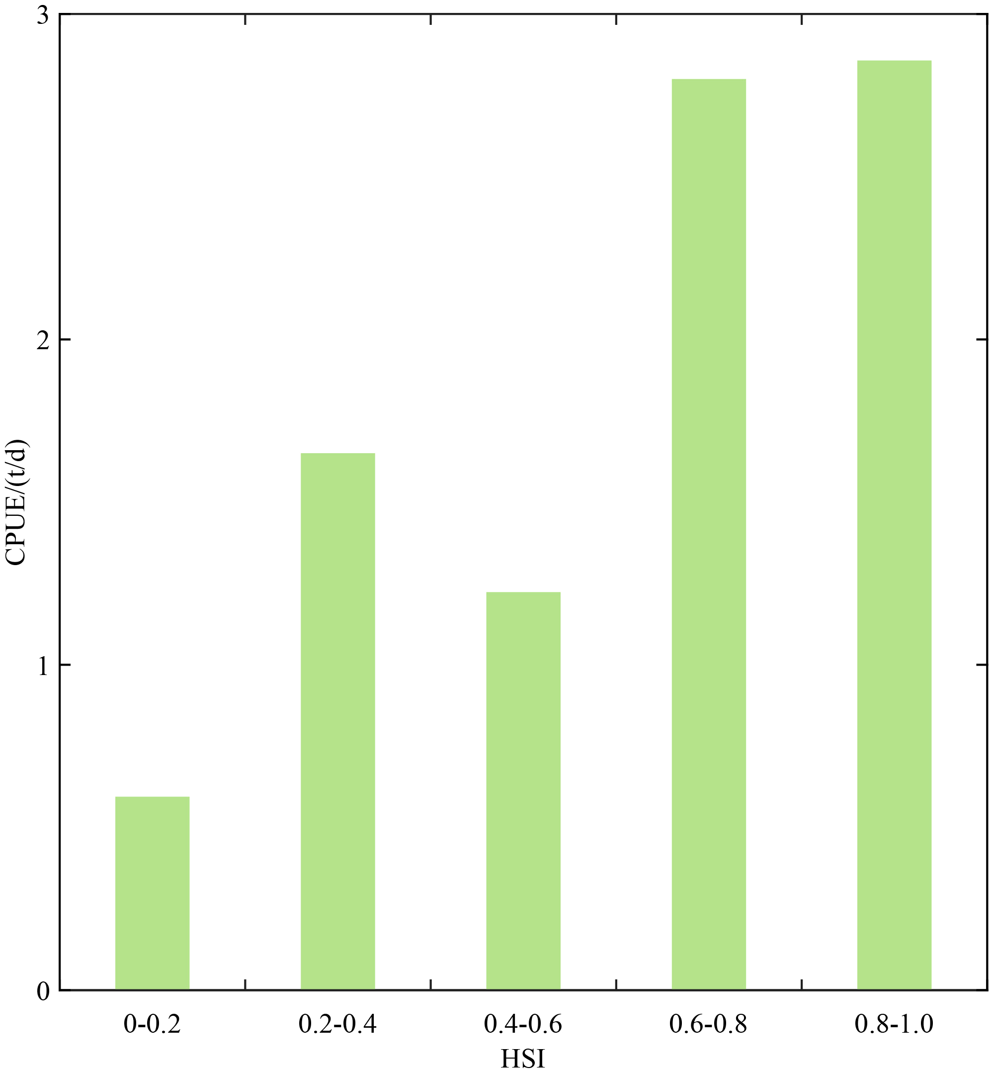
Mean catch per unit effort (CPUE) corresponding to each interval of habitat suitability index (HSI) under the optimal HSI model (case 6) from 2019 to 2021.
3.2 The abundance of D. gigas within CEs and AEs
Figure 4 illustrated the distribution of D. gigas CPUE within different types of eddies. In AEs, the median CPUE was 2.7 t/d, with a mean value of 3.64 t/d. In CEs, the median CPUE was 3.6 t/d, and the mean value was 4.26 t/d. The t-test results indicated that there was a significant difference in the CPUE of D. gigas within CEs and AEs (P<0.001).
Figure 4
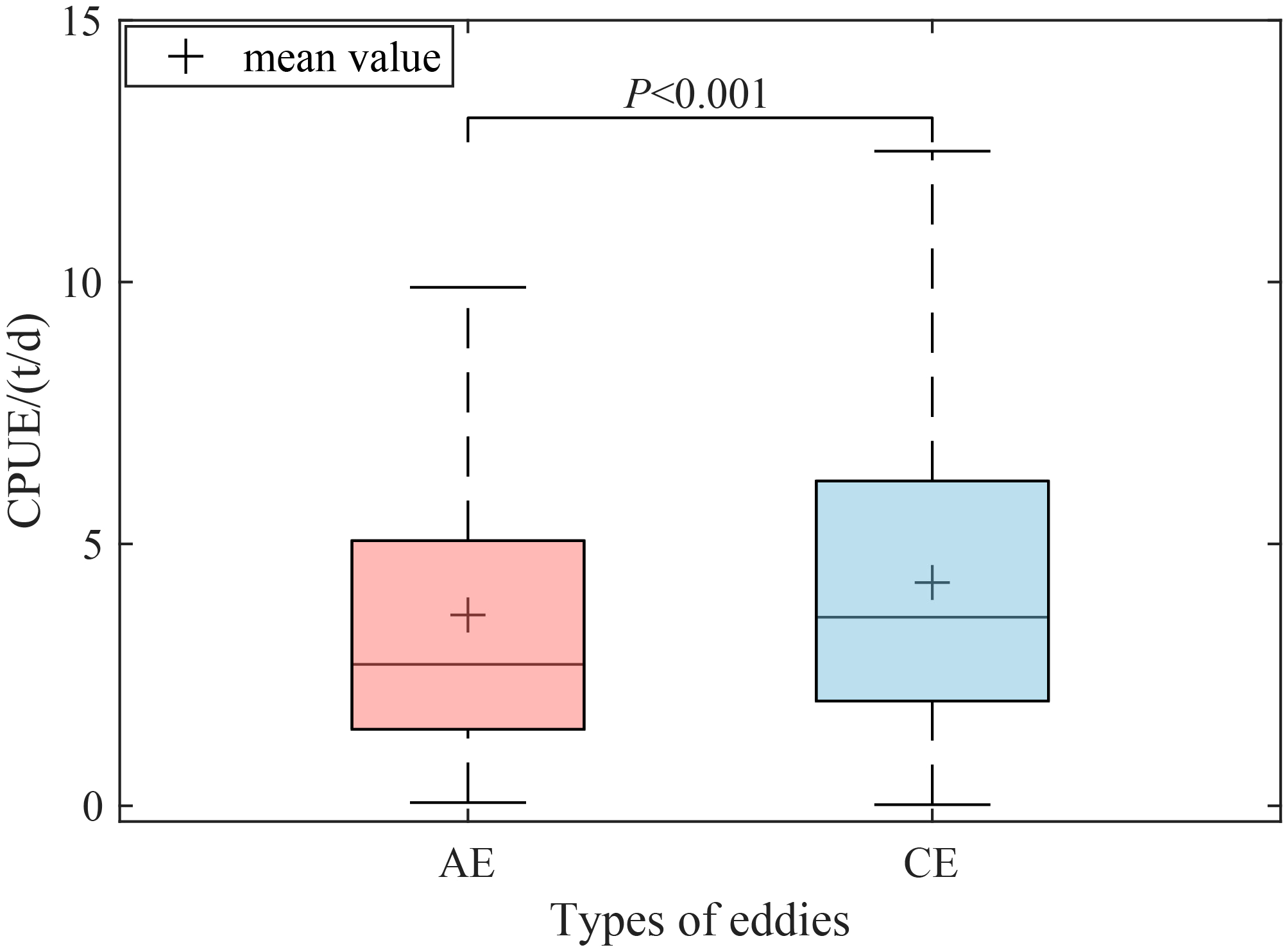
Comparison of catch per unit effort (CPUE) between anticyclonic (AE) and cyclonic eddy (CE).
3.3 Distribution of habitat suitability and its interannual variability for D. gigas in CEs and AEs
The distribution patterns of mean HSI, SISST, SIChl-a, and SIDO within eddies of different polarities were shown in Figure 5A. In CEs, the mean SIDO ranged from 0.32 to 0.58, while in AEs, it ranged from 0.26 to 0.45. The mean SISST did not exceed 0.6 in either CEs or AEs. Both the number of grids with mean HSI and mean SIChl-a greater than 0.6 were higher in CEs compared to AEs.
Figure 5
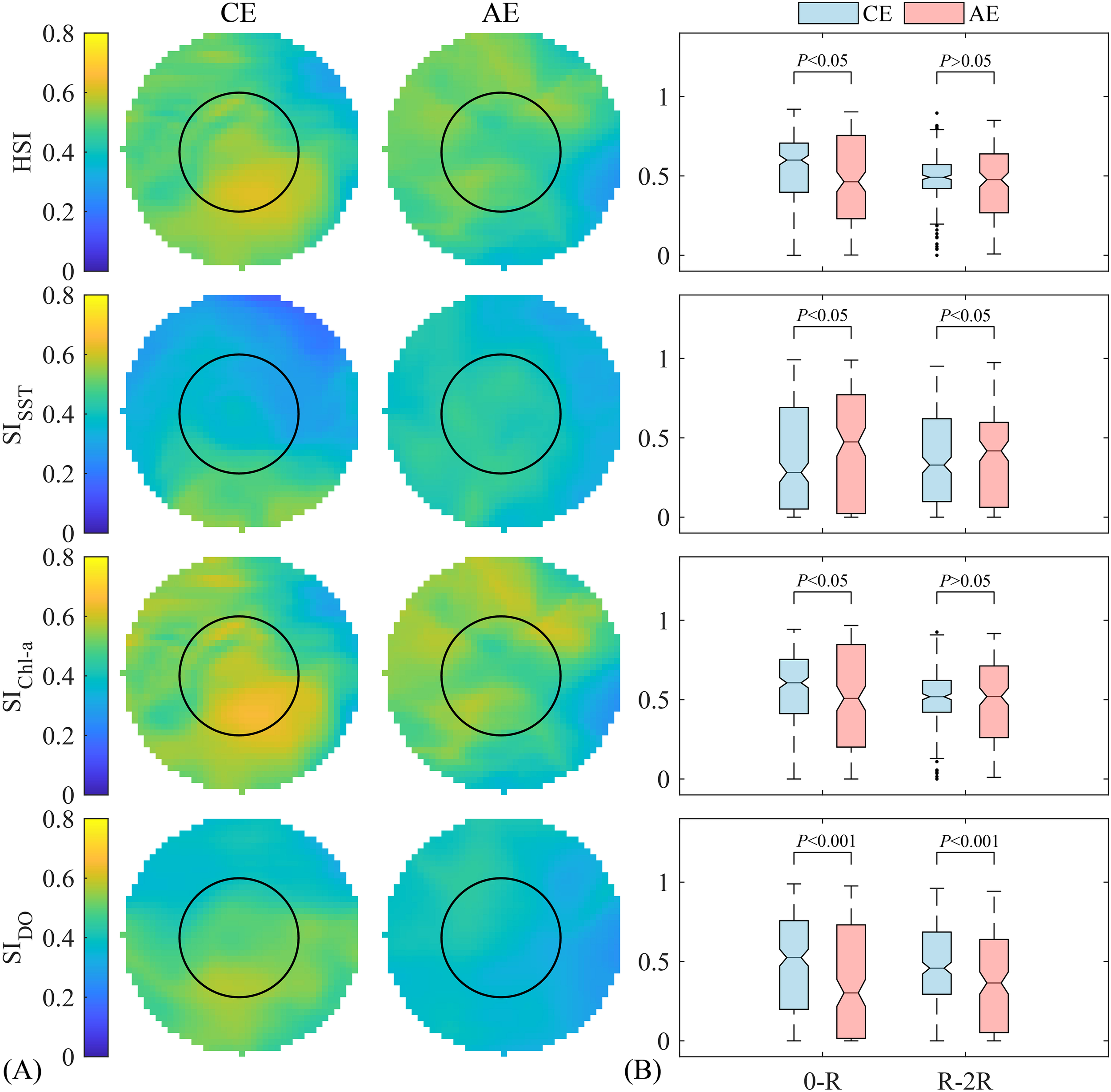
(A) Comparison of the average suitability index values for each environmental factor and the average habitat suitability index (HSI) for Dosidicus gigas between cyclonic (CE) and anticyclonic eddy (AE) (the black solid line represents the inner circle from the center to R); (B) Boxplot comparison of the mean habitat suitability index (HSI) and single-factor suitability index (SI) in different regions of the eddies (the 0-R region is the inner circle from the center to R, the R-2R region is the annular zone extending from R to 2R, R is half the radius of the standardized circular grid).
The mean HSI, SISST, SIChl-a, and SIDO in different eddy regions were presented in Figure 5B. In the 0-R region, CEs exhibited significantly higher HSI, SIChl-a (P<0.05), and SIDO than AEs, while the SISST was significantly lower (P<0.05). In the R-2R region, there was not a significant difference between the two eddy types in the HSI and SIChl-a (P>0.05); however, CEs exhibited a significantly lower SISST and a higher SIDO than AEs (P<0.05).
Figure 6 showed the relationship between the proportion of suitable HSI and the distance from the eddy center. Overall, the proportion of suitable HSI decreased with increasing distance from the eddy core in both CEs and AEs. In CEs, the proportion peaked at 57.5% (0.1 R) and dropped to 44.8% (2.0 R), while in AEs, the highest proportion was 51.3% (0.6 R) and the lowest was 41.7% (1.9 R).
Figure 6
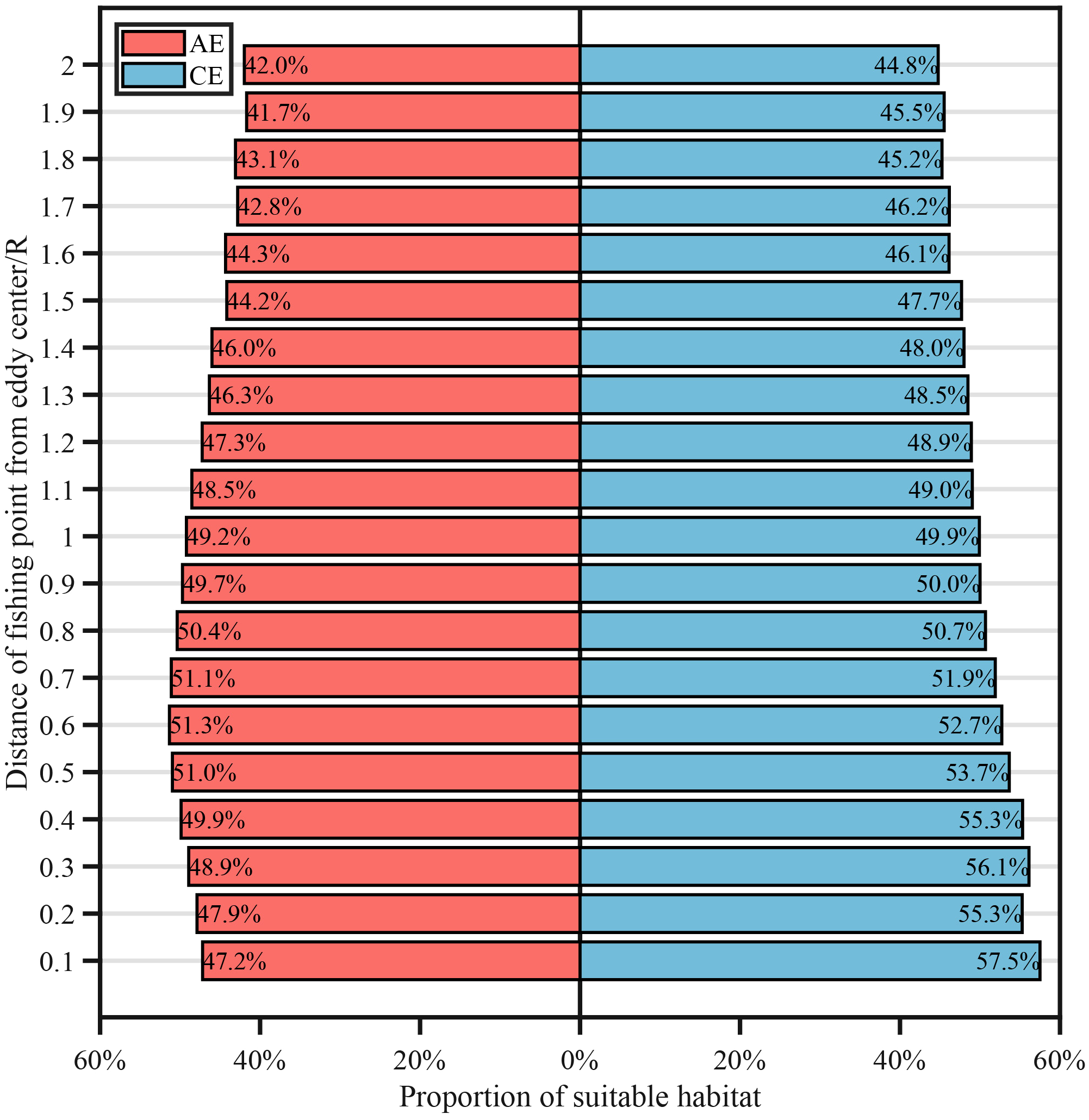
Proportion of suitable habitat in cyclonic (CE) and anticyclonic eddy (AE) at varying distances from eddies centers.
Differences in D. gigas habitat suitability between the two eddy types from 2015 to 2020 are depicted in Figure 7. Overall, HSI values in both CEs and AEs exhibited notable interannual variability. In most years, the core regions of CEs showed relatively high HSI values, especially in 2019 and 2020. In 2016, 2017, and 2020, AEs also displayed relatively high HSI values. However, in 2018, habitat suitability was relatively poor within both eddy types.
Figure 7
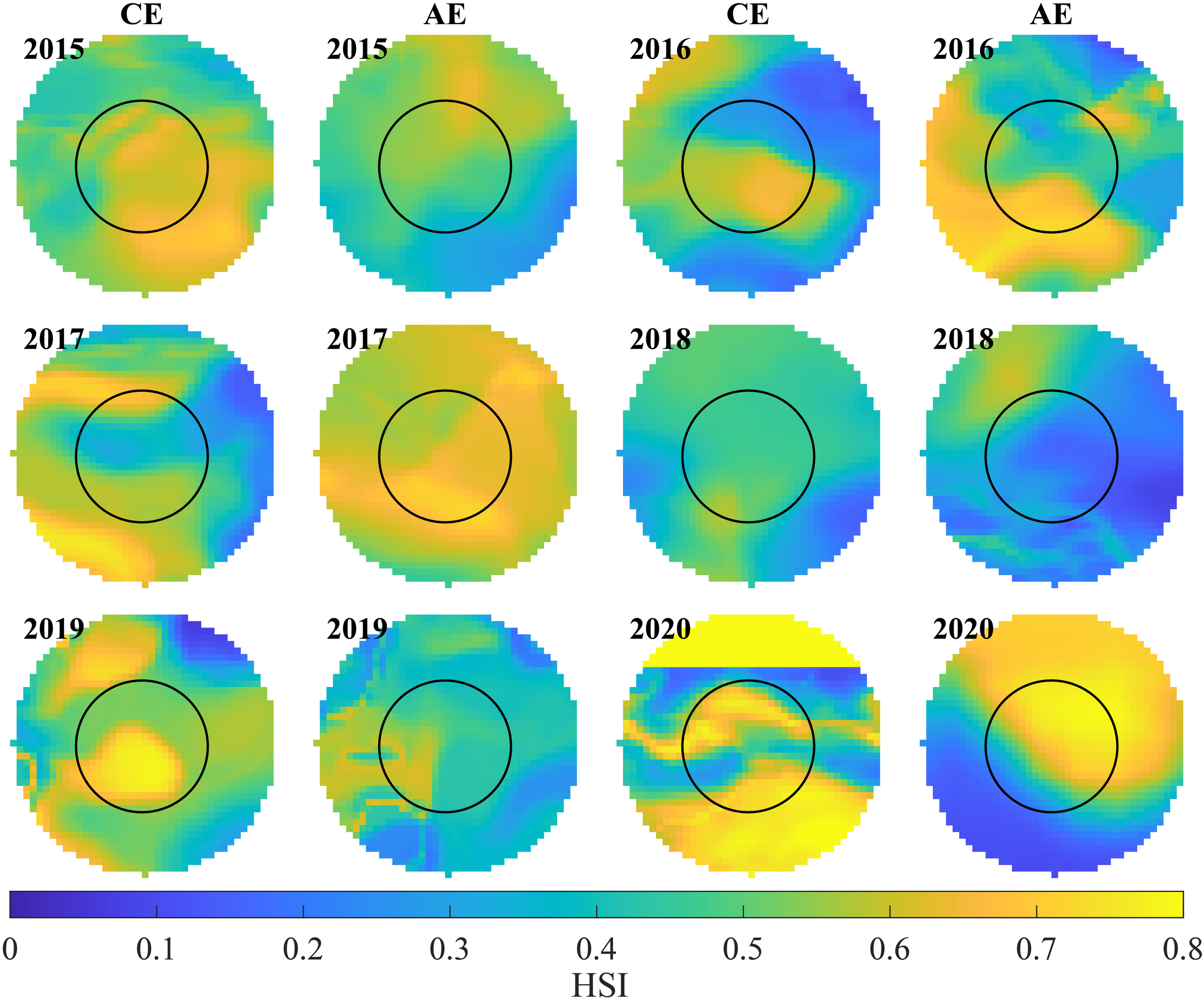
Comparison of Dosidicus gigas habitat suitability between cyclonic (CE) and anticyclonic eddy (AE) from 2015 to 2020 (the black solid line represents the inner circle from the center to R).
3.4 Influence of eddy parameters on habitat suitability for D. gigas
The deviance explained by the GAM model constructed based on AE data was 41.3%, whereas the deviance explained by the GAM model constructed based on CE data was 30.9%. The GAM results revealed that radius, velocity, and amplitude all exerted significant effects on the habitat suitability of D. gigas(Figure 8). When the radius of CEs ranged from approximately 50 to 125 km, the confidence interval was relatively narrow, and the HSI increased with the radius. In contrast, for AEs, when the radius was approximately 45 to 60 km, the confidence interval was narrower, and the HSI decreased as the radius increased. In CEs, HSI increased with rising velocity, peaking at approximately 0.15 m/s before gradually declining. Conversely, in AEs, HSI tended to mainly decrease as rotational speed increased. Regarding amplitude, HSI in AEs first increased and then declined as amplitude increased, whereas in CEs, HSI progressively decreased as amplitude increased.
Figure 8
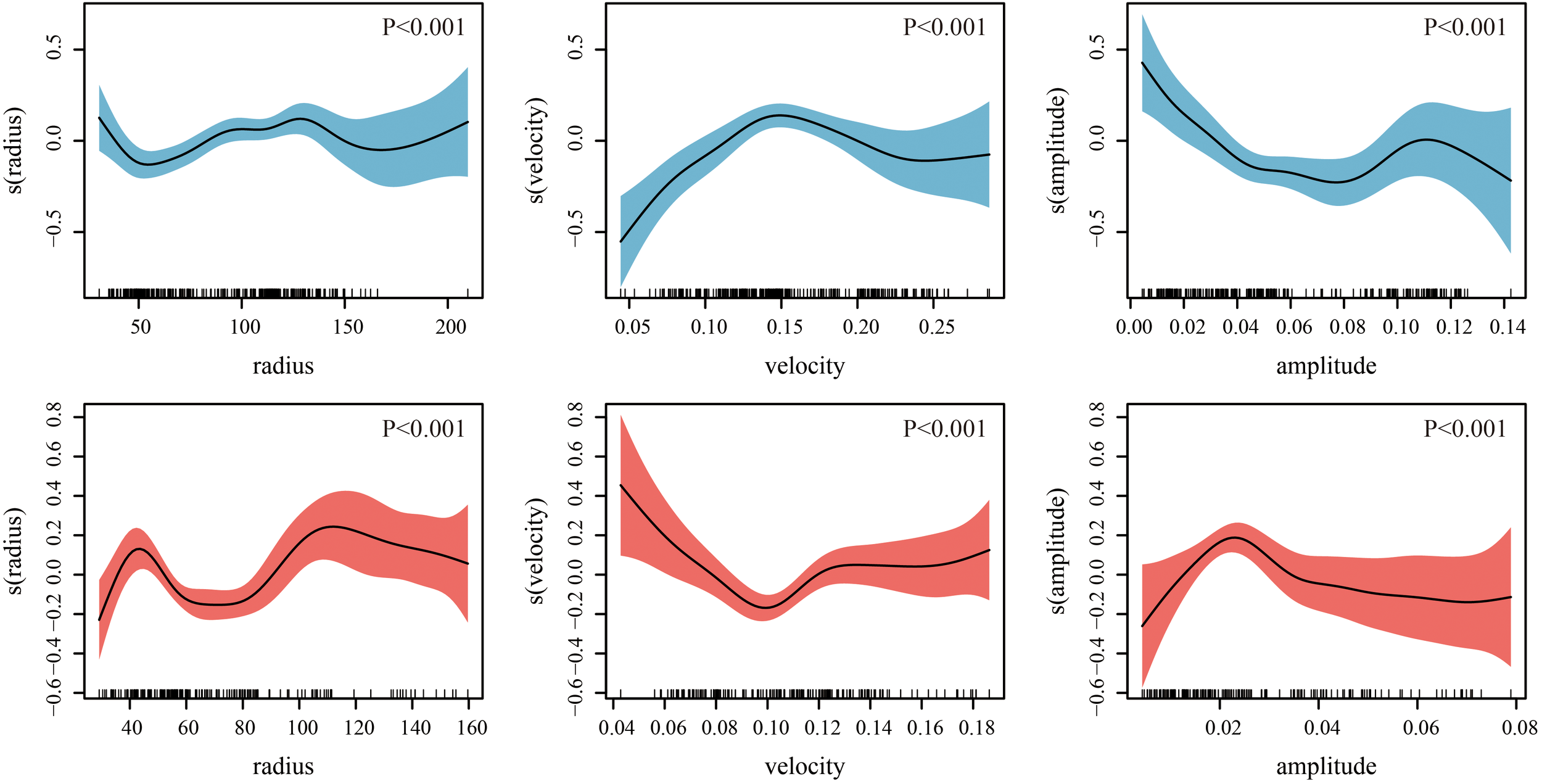
The influence of eddy parameters on the mean habitat suitability index (HSI) of Dosidicus gigas within their impact range (lower panel, anticyclonic eddies; upper panel, cyclonic eddies).
4 Discussion
Habitat quality directly influences the presence and abundance of marine organisms. Understanding the spatial and temporal dynamics of habitats is critical for sustaining biological resources. Numerous models have been developed to identify and predict marine species’ habitat distributions, such as the MaxEnt model (Jones et al., 2012), neural network models (Lin et al., 2023), and generalized additive mixed models (Wang et al., 2023). Compared to these, the HSI model is valued for its simplicity, transparency, speed, and reliability, and it has been widely applied in wildlife management (Li et al., 2014). In this study, squid fishing effort data and environmental variables were used as inputs to construct the HSI model. A previous study on Pacific squid demonstrated that HSI models based on CPUE tend to incorrectly estimate suitable habitat areas and their monthly variability compared to those constructed using fishing effort (Tian et al., 2009). The structure of the HSI model also plays a decisive role in its predictive accuracy. Various methods exist to combine individual SI models into an overall HSI, such as multiplicative, hybrid, geometric mean, and arithmetic mean approaches (Gong et al., 2011). Each approach yields different HSI values. Although the geometric and arithmetic means are commonly used (Tian et al., 2009; Yu et al., 2015), they assume equal species responses to all environmental factors and may fail to accurately capture habitat suitability. To address this limitation, this study applied 25 different weighting schemes (Supplementary Table S1) for the SI model, evaluated their performance, and selected the optimal configuration for predicting D. gigas habitat suitability.
In this study, the constructed SI models exhibited a clear normal distribution (P < 0.001) (Table 1) and showed strong consistency with the observed SI values (Figure 2), indicating that the models effectively quantified the suitability of D. gigas in relation to the selected environmental variables. Moreover, we observed monthly fluctuations in the suitable ranges of DO, SST, and Chl-a for D. gigas, which aligns with findings from previous studies (Wen et al., 2024; Yu et al., 2015). These variations reflect that the D. gigas are at different life history stages in different months and differ in their needs for the three environmental factors. DO, SST, and Chl-a represent metabolic constraints, thermal conditions, and food availability, respectively, and exert significant influences on the spatial distribution of D. gigas (Yu et al., 2025). The optimal weighting scheme for SIDO, SISST, and SIChl-a was determined to be 0.1:0.1:0.8 (Supplementary Table S2), highlighting the dominant role of Chl-a in shaping D. gigas habitats during March-May. This period corresponds to one of the key spawning seasons of D. gigas off Chile (Ibáñez et al., 2016), during which their energy demands rely heavily on feeding (Yu et al., 2025). Given the potential positive relationship between Chl-a and the foraging environment of D. gigas (Ichii et al., 2002), the higher weight assigned to SIChl-a in our model appears justified. In contrast, a previous study (Wen et al., 2024) found that SST contributed more to D. gigas habitat formation than Chl-a in the eastern equatorial Pacific during the same season, suggesting that habitat formation mechanisms for the same species may vary across different regions. The HSI model validation results (Figure 3) further demonstrated that D. gigas were predominantly distributed within areas classified as suitable habitats, underscoring the model’s high predictive accuracy.
Mesoscale eddies profoundly influence the distribution of organisms across different trophic levels in marine food webs (Ueno et al., 2023). Owing to the contrasting current structures within CEs and AEs, various marine species exhibit distinct aggregation preferences in these eddies, and such patterns are often modulated by geographic location (Xing et al., 2023, 2024). For instance, compared to CEs, blue marlin, albacore tuna, blue sharks, and king penguins are more frequently observed aggregating within AEs (Arostegui et al., 2022; Braun et al., 2019; Cotté et al., 2007). In this study, however, analysis of multi-year autumn catch data for D. gigas off Chile, combined with mesoscale eddy datasets, revealed that CEs supported higher abundances of D. gigas relative to AEs (Figure 4). CEs promote upwelling and AEs induce downwelling in both hemispheres—the direction of rotation is reversed between them. In the Southern Hemisphere, CEs rotate clockwise and AEs counter-clockwise, whereas in the Northern Hemisphere, the opposite occurs. These opposing dynamics distinctly modulate local DO, SST, and Chl-a conditions (Bakun, 2006), thereby creating habitat environments of differing quality within their influence zones. A comparison of D. gigas suitability for DO, SST, and Chl-a within the two eddy types (Figure 5) showed that CEs had a higher proportion of suitable SIChl-a and SIDO, while SISST proportions were slightly lower than in AEs. The combined effects of these three factors suggest that CEs provide more favorable habitats for D. gigas. Previous studies have also documented interannual variability in D. gigas habitat suitability within eddies (Jin et al., 2024b) and reported that the proportion of suitable habitats changes with distance from the eddy core (Jin et al., 2024a). Similar patterns were observed in our analysis (Figures 6, 7), likely driven by interannual fluctuations in oceanic conditions and energy differences across eddy regions. Eddy amplitude typically reflects its intensity, radius indicates its area of influence, and velocity reflects energy distribution and developmental dynamics (Cui et al., 2025). This study found that the quality of D. gigas habitats within eddies was significantly influenced by eddy radius, velocity, and amplitude (Figure 8). For example, the HSI within CEs was higher when the velocity was approximately 0.15 m/s, while HSI within AEs was lower when the velocity was around 0.10 m/s. The study hypothesizes that variations in eddy parameters may alter the distribution of water masses and the material transport capacity within the eddy, thereby driving changes in environmental factors and influencing the habitat suitability for D. gigas.
This study employed HSI models with varying weightings to investigate differences in the abundance and habitat of D. gigas within CEs and AE off Chile during austral autumn. The results revealed that, compared to AEs, the suitable DO and Chl-a conditions within CEs facilitated the formation of high-quality habitats for D. gigas, leading to substantial aggregations of this species. However, the study has certain limitations. It did not account for the direct effects of upwelling and downwelling within mesoscale eddies on D. gigas, nor did it explore the mechanisms of eddy parameter effects on habitat suitability for D. gigas or consider the impacts of climate change on both eddies and squid populations. Future research should incorporate additional physical, biological, and climatic factors, along with more advanced models, such as convolutional neural networks, to explore species distribution changes driven by eddy-induced environmental factors. Overall, these findings offer novel insights into the ecological effects of mesoscale eddies on cephalopod species and provide a scientific basis for their sustainable management.
Statements
Data availability statement
The original contributions presented in the study are included in the article/Supplementary Material. Further inquiries can be directed to the corresponding author.
Ethics statement
The manuscript presents research on animals that do not require ethical approval for their study.
Author contributions
XW: Conceptualization, Formal Analysis, Methodology, Visualization, Writing – original draft. PJ: Conceptualization, Writing – original draft. WY: Conceptualization, Funding acquisition, Writing – original draft, Writing – review & editing.
Funding
The author(s) declare financial support was received for the research and/or publication of this article. This study was financially supported by the 2024 International Cooperation Seed Funding Project for China’s Ocean Decade Actions (GHZZ3702840002024020000024), the AI Special Program of Shanghai Municipal Education Commission for Wei Yu in Shanghai Ocean University (A1-3405-25-000303), Shanghai talent development funding for the project (2021078), and the Natural Science Foundation of Shanghai (23ZR1427100).
Conflict of interest
The authors declare that the research was conducted in the absence of any commercial or financial relationships that could be construed as a potential conflict of interest.
Generative AI statement
The author(s) declare that no Generative AI was used in the creation of this manuscript.
Any alternative text (alt text) provided alongside figures in this article has been generated by Frontiers with the support of artificial intelligence and reasonable efforts have been made to ensure accuracy, including review by the authors wherever possible. If you identify any issues, please contact us.
Publisher’s note
All claims expressed in this article are solely those of the authors and do not necessarily represent those of their affiliated organizations, or those of the publisher, the editors and the reviewers. Any product that may be evaluated in this article, or claim that may be made by its manufacturer, is not guaranteed or endorsed by the publisher.
Supplementary material
The Supplementary Material for this article can be found online at: https://www.frontiersin.org/articles/10.3389/fmars.2025.1669638/full#supplementary-material
References
1
Alabia I. D. Saitoh S.-I. Mugo R. Igarashi H. Ishikawa Y. Usui N. et al . (2015). Identifying pelagic habitat hotspots of neon flying squid in the temperate waters of the central north pacific. PloS One10, e0142885. doi: 10.1371/journal.pone.0142885
2
Arostegui M. C. Gaube P. Woodworth-Jefcoats P. A. Kobayashi D. R. Braun C. D. (2022). Anticyclonic eddies aggregate pelagic predators in a subtropical gyre. Nature609, 535–540. doi: 10.1038/s41586-022-05162-6
3
Bakun A. (2006). Fronts and eddies as key structures in the habitat of marine fish larvae: opportunity, adaptive response and competitive advantage. Sci. Mar.70, 105–122. doi: 10.3989/scimar.2006.70s2105
4
Bian C. Jing Z. Wang H. Wu L. Chen Z. Gan B. et al . (2023). Oceanic mesoscale eddies as crucial drivers of global marine heatwaves. Nat. Commun.14, 2970. doi: 10.1038/s41467-023-38811-z
5
Braun C. D. Gaube P. Sinclair-Taylor T. H. Skomal G. B. Thorrold S. R. (2019). Mesoscale eddies release pelagic sharks from thermal constraints to foraging in the ocean twilight zone. Proc. Natl. Acad. Sci.116, 17187–17192. doi: 10.1073/pnas.1903067116
6
Chaigneau A. Eldin G. Dewitte B. (2009). Eddy activity in the four major upwelling systems from satellite altimetry, (1992–2007). Prog. Oceanogr.83, 117–123. doi: 10.1016/j.pocean.2009.07.012
7
Chelton D. B. Schlax M. G. Samelson R. M. (2011). Global observations of nonlinear mesoscale eddies. Prog. Oceanogr.91, 167–216. doi: 10.1016/j.pocean.2011.01.002
8
Chelton D. B. Schlax M. G. Samelson R. M. de Szoeke R. A. (2007). Global observations of large oceanic eddies. Geophys. Res. Lett.34. doi: 10.1029/2007GL030812
9
Chen X. Li G. Feng B. Tian S. (2009). Habitat suitability index of chub mackerel (Scomber japonicus) from July to September in the east China sea. J. Oceanogr.65, 93–102. doi: 10.1007/s10872-009-0009-9
10
Chen X. Liu B. Chen Y. (2008). A review of the development of Chinese distant-water squid jigging fisheries. Fish. Res.89, 211–221. doi: 10.1016/j.fishres.2007.10.012
11
Cotté C. Park Y.-H. Guinet C. Bost C.-A. (2007). Movements of foraging king penguins through marine mesoscale eddies. Proc. R. Soc B: Biol. Sci.274, 2385–2391. doi: 10.1098/rspb.2007.0775
12
Covington J. Chen N. Wiggins S. Lunasin E. (2025). Probabilistic eddy identification with uncertainty quantification. Physica D473, 134542. doi: 10.1016/j.physd.2025.134542
13
Cui A. Zhang Z. Yan H. Han B. (2025). Spatial and temporal characteristics of mesoscale eddies in the north Atlantic Ocean based on SWOT mission. Remote Sens.17, 1469. doi: 10.3390/rs17081469
14
Davis R. W. Ortega-Ortiz J. G. Ribic C. A. Evans W. E. Biggs D. C. Ressler P. H. et al . (2002). Cetacean habitat in the northern oceanic gulf of Mexico. Deep Sea Res. Part I, 49, 121–142. doi: 10.1016/S0967-0637(01)00035-8
15
Della Penna A. Llort J. Moreau S. Patel R. Kloser R. Gaube P. et al . (2022). The impact of a Southern ocean cyclonic eddy on mesopelagic micronekton. J. Geophys. Res.: Oceans127, e2022JC018893. doi: 10.1029/2022jc018893
16
Feng Z. Chen B. Yu W. Chen X. (2025). Prediction of habitat and abundance of Dosidicus gigas off Chile under different climate scenarios. Trans. Oceanol. Limnol.47, 136–145.
17
Feng Z. Yu W. Zhang Y. Li Y. Chen X. (2022). Habitat variations of two commercially valuable species along the Chilean waters under different-intensity El Niño events. Front. Mar. Sci.9. doi: 10.3389/fmars.2022.919620
18
Frenger I. Gruber N. Knutti R. Münnich M. (2013). Imprint of Southern ocean eddies on winds, clouds and rainfall. Nat. Geosci.6, 608–612. doi: 10.1038/ngeo1863
19
Gong C. Chen X. Gao. F. Guan W. Lei. L. (2011). Review on habitat suitability index in fishery science. J. shanghai ocean Univ.20, 260–269.
20
Han H. Yang C. Zhang H. Fang Z. Jiang B. Su B. et al . (2022). Environment variables affect CPUE and spatial distribution of fishing grounds on the light falling gear fishery in the northwest Indian Ocean at different time scales. Front. Mar. Sci.9. doi: 10.3389/fmars.2022.939334
21
Hightower J. E. Harris J. E. Raabe J. K. Brownell P. Drew C. A. (2012). A Bayesian spawning habitat suitability model for American shad in southeastern United States rivers. J. Fish Wildl. Manage.3, 184–198. doi: 10.3996/082011-JFWM-047
22
Ibáñez C. M. Sepúlveda R. D. Ulloa P. Keyl F. Pardo-Gandarillas M. C. (2016). The biology and ecology of the jumbo squid Dosidicus gigas (cephalopoda) in Chilean waters: a review. Lat. Am. J. Aquat. Res.43, 402–414. doi: 10.3856/vol43-issue3-fulltext-2
23
Ichii T. Mahapatra K. Watanabe T. Yatsu A. Inagake D. Okada Y. (2002). Occurrence of jumbo flying squid Dosidicus gigas aggregations associated with the countercurrent ridge off the Costa Rica dome during 1997 el niño and 1999 La niña. Mar. Ecol. Prog. Ser.231, 151–166. doi: 10.3354/meps231151
24
Jin P. Fan J. Wu X. Du Y. Yu W. (2024a). Jumbo Flying Squid Distribution within Anticyclonic Eddies under Anomalous Climatic Conditions. Ecosyst. Health Sustain10, 177. doi: 10.34133/ehs.0177
25
Jin P. Zhang Y. Du Y. Chen X. Kindong R. Xue H. et al . (2024b). Eddy impacts on abundance and habitat distribution of a large predatory squid off Peru. Mar. Environ. Res.195, 106368. doi: 10.1016/j.marenvres.2024.106368
26
Jones M. C. Dye S. R. Pinnegar J. K. Warren R. Cheung W. W. L. (2012). Modelling commercial fish distributions: prediction and assessment using different approaches. Ecol. Modell.225, 133–145. doi: 10.1016/j.ecolmodel.2011.11.003
27
Li G. Chen X. Lei L. Guan W. (2014). Distribution of hotspots of chub mackerel based on remote-sensing data in coastal waters of China. Int. J. Remote Sens.35, 4399–4421. doi: 10.1080/01431161.2014.916057
28
Li X. Gan B. Zhang Z. Cao Z. Qiu B. Chen Z. et al . (2025). Oceanic uptake of CO2 enhanced by mesoscale eddies. Sci. Adv.11, eadt4195. doi: 10.1126/sciadv.adt4195
29
Lin H. Wang J. Zhu J. Chen X. (2023). Evaluating the impacts of environmental and fishery variability on the distribution of bigeye tuna in the Pacific Ocean. ICES J. Mar. Sci.80, 2642–2656. doi: 10.1093/icesjms/fsad163
30
Ma X. Chang P. Saravanan R. Montuoro R. Hsieh J.-S. Wu D. et al . (2015). Distant influence of Kuroshio eddies on north pacific weather patterns? Sci. Rep.5, 17785. doi: 10.1038/srep17785
31
McGillicuddy D. J. (2016). Mechanisms of physical-biological-biogeochemical interaction at the oceanic mesoscale. Annu. Rev. Mar. Sci.8, 125–159. doi: 10.1146/annurev-marine-010814-015606
32
National Research Council (1982). Impacts of emerging agricultural trends on fish and wildlife habitat (Washington, DC: National Academy Press).
33
Nieto K. McClatchie S. Weber E. D. Lennert-Cody C. E. (2014). Effect of mesoscale eddies and streamers on sardine spawning habitat and recruitment success off southern and central California. J. Geophys. Res.: Oceans119, 6330–6339. doi: 10.1002/2014JC010251
34
Nigmatullin C. (2001). A review of the biology of the jumbo squid Dosidicus gigas (cephalopoda: Ommastrephidae). Fish. Res.54, 9–19. doi: 10.1016/s0165-7836(01)00371-x
35
O’brien R. M. (2007). A caution regarding rules of thumb for variance inflation factors. Qual Quant41, 673–690. doi: 10.1007/s11135-006-9018-6
36
Pegliasco C. Delepoulle A. Mason E. Morrow R. Faugère Y. Dibarboure G. (2022). META3.1exp: a new global mesoscale eddy trajectory atlas derived from altimetry. Earth Syst. Sci. Data14, 1087–1107. doi: 10.5194/essd-14-1087-2022
37
Tian S. Chen X. Chen Y. Xu L. Dai X. (2009). Evaluating habitat suitability indices derived from CPUE and fishing effort data for Ommatrephes bratramii in the northwestern Pacific Ocean. Fish. Res.95, 181–188. doi: 10.1016/j.fishres.2008.08.012
38
Ueno H. Bracco A. Barth J. A. Budyansky M. V. Hasegawa D. Itoh S. et al . (2023). Review of oceanic mesoscale processes in the north pacific: physical and biogeochemical impacts. Prog. Oceanogr.212, 102955. doi: 10.1016/j.pocean.2022.102955
39
Vinagre C. Fonseca V. Cabral H. Costa M. J. (2006). Habitat suitability index models for the juvenile soles, Solea solea and Solea Senegalensis, in the Tagus estuary: defining variables for species management. Fish. Res.82, 140–149. doi: 10.1016/j.fishres.2006.07.011
40
Wang J. Chen X. Li Y. Boenish R. (2023). The effects of climate-induced environmental variability on Pacific Ocean squids. ICES J. Mar. Sci.80, 878–888. doi: 10.1093/icesjms/fsad016
41
Wen L. Zhang H. Fang Z. Chen X. (2025). The effects of climate change on sthenoteuthis oualaniensis habitats in the northern Indian Ocean. Animals15, 573. doi: 10.3390/ani15040573
42
Wen J. Zhou Z. Zhang Y. Yu W. Chen B. Chen X. (2024). Climate-related habitat variations of Humboldt squid in the eastern equatorial Pacific Ocean. J. Mar. Syst.243, 103960. doi: 10.1016/j.jmarsys.2023.103960
43
Wu X. Jin P. Yu W. (2025). The relationship between mesoscale eddies and the abundance and distribution of jumbo flying squid off Chile. Front. Mar. Sci.12. doi: 10.3389/fmars.2025.1575299
44
Wunsch C. Ferrari R. (2004). Vertical mixing, energy and the general circulation of the oceans. Annu. Rev. Fluid Mech.36, 281–314. doi: 10.1146/annurev.fluid.36.050802.122121
45
Xing Q. Yu H. Wang H. Ito S. Chai F. (2023). Mesoscale eddies modulate the dynamics of human fishing activities in the global midlatitude ocean. Fish Fish.24, 527–543. doi: 10.1111/faf.12742
46
Xing Q. Yu H. Wang H. Ito S. Yu W. (2024). Mesoscale eddies exert inverse latitudinal effects on global industrial squid fisheries. Sci. Total Environ. 950, 175211. doi: 10.1016/j.scitotenv.2024.175211
47
Yu W. Chen X. Yi Q. Chen Y. Zhang Y. (2015). Variability of suitable habitat of western winter-spring cohort for neon flying squid in the northwest pacific under anomalous environments. PloS One10, e0122997. doi: 10.1371/journal.pone.0122997
48
Yu W. Feng X. Wen J. Wu X. Fang X. Cui J. et al . (2025). The potential impacts of climate change on the life history and habitat of jumbo flying squid in the southeast Pacific Ocean: overview and implications for fisheries management. Rev. Fish Biol. Fish.35, 707–731. doi: 10.1007/s11160-025-09929-8
49
Zhang S. Shi J. Cao X. (2025). Impact of mesoscale eddies on acoustic propagation under a rough sea surface. Remote Sens.17, 2036. doi: 10.3390/rs17122036
50
Zhou K. Benitez-Nelson C. R. Huang J. Xiu P. Sun Z. Dai M. (2021). Cyclonic eddies modulate temporal and spatial decoupling of particulate carbon, nitrogen, and biogenic silica export in the north pacific subtropical gyre. Limnol. Oceanogr.66, 3508–3522. doi: 10.1002/lno.11895
Summary
Keywords
Dosidicus gigas , mesoscale eddy, habitat assessment, abundance, the waters off Chile
Citation
Wu X, Jin P and Yu W (2025) Identify habitat distribution within the mesoscale eddies for jumbo flying squid off Chilean waters. Front. Mar. Sci. 12:1669638. doi: 10.3389/fmars.2025.1669638
Received
20 July 2025
Accepted
22 September 2025
Published
03 October 2025
Volume
12 - 2025
Edited by
Fabio Fiorentino, National Research Council (CNR), Italy
Reviewed by
Bernardo Patti, National Research Council (CNR), Italy; Xiaodi Gao, East China Sea Fisheries Research Institute, China
Updates
Copyright
© 2025 Wu, Jin and Yu.
This is an open-access article distributed under the terms of the Creative Commons Attribution License (CC BY). The use, distribution or reproduction in other forums is permitted, provided the original author(s) and the copyright owner(s) are credited and that the original publication in this journal is cited, in accordance with accepted academic practice. No use, distribution or reproduction is permitted which does not comply with these terms.
*Correspondence: Wei Yu, wyu@shou.edu.cn
Disclaimer
All claims expressed in this article are solely those of the authors and do not necessarily represent those of their affiliated organizations, or those of the publisher, the editors and the reviewers. Any product that may be evaluated in this article or claim that may be made by its manufacturer is not guaranteed or endorsed by the publisher.