Enhancing sensor accuracy in mobile multi-sensor systems for atmospheric monitoring using disturbance observer and sensor estimators

Recent progress in marine environmental monitoring has underscored the importance of equally rigorous atmospheric observations, and it has consequently focused on developing mobile sensors that improve data collection accuracy and operational flexibility. unmanned aerial vehicles (UAVs) are attractive carriers owing to their low cost and operational agility; however, the stringent size–and–weight constraints imposed on onboard sensors often translate into poor accuracy, especially under rapidly fluctuating ambient temperatures. This paper introduces a compact, lightweight composite sensor payload – readily integrable with UAVs – that preserves measurement precision down to −40°C by embedding a disturbance observer (DOB)–based compensation algorithm directly in the sensor micro–controller, using externally sensed air temperature (via an insulated probe) as baseline data for onboard correction. The DOB continuously estimates and cancels temperature–induced bias and electromagnetic interference in real time, without hardware redundancy or external calibration during operation. High–altitude test–chamber experiments show that the proposed system lowers the temperature RMSE from 28.67°C to 15.74°C and raises the coefficient of determination (R²) from 0.02 to 0.76. These results confirm that DOB–assisted correction substantially enhances the robustness and reliability of lightweight UAV–compatible sensors, paving the way for high–resolution coastal–and–open–ocean ground–to–stratosphere profiling that supports coupled air–sea flux assessments for marine exploration.

1 Introduction

Recent advancements in atmospheric environmental monitoring have focused on the development of small mobile sensors to improve data-collection accuracy and operational flexibility. Equally important, a growing body of marine-climatology literature shows that atmospheric processes directly regulate upper-ocean heat content. Notably, Günther et al. (2024) demonstrate that stratospheric aerosol forcing can cool the western Pacific warm pool on sub-seasonal timescales, underscoring the need for in-situ observations that capture atmospheric and oceanic states concurrently.

Fixed-point observatories—land stations, moored buoys, and shipborne packages—struggle to sample these tightly coupled air-sea processes with adequate spatial and vertical resolution. Because conventional sensors are configured for fixed sites, synoptic three-dimensional observations remain essential for constraining pollution sources and energy-flux pathways across both land and sea.

Mobile platforms therefore constitute a practical means of extending the reach of environmental sensors. Small unmanned aerial vehicles UAVs have emerged as flexible observational platforms. Fekih et al. (2021) developed and evaluated a mobile participatory system for monitoring air-quality and urban-heat-island conditions with cost-effective miniature sensors, emphasizing data validation and energy efficiency through comparisons with reference instruments. Chen et al. (2021) compiled a high-resolution, vision-based air quality dataset using UAVs to capture wide-swath imagery paired with ground sensors, thereby improving the spatial interpolation of air-quality fields.

Concas et al. (2021) catalog state-of-the-art machine-learning calibration methods for inexpensive air-quality sensors; however, they note that these approaches depend on large labeled datasets and remain largely unvalidated in the steep temperature and pressure gradients encountered during rapid UAV profiling sorties. Recent assessments further document bias and drift of low-cost sensors under changing T/p/RH, reinforcing the need for calibration schemes that remain valid off the training envelope (Siddiqui et al., 2025; Hayward et al., 2024).

Zappa et al. (2020) demonstrated ship-launched VTOL UAVs equipped with multispectral imagers and microbuoys, capable of resolving centimeter-scale sea-surface variability while simultaneously profiling the marine atmospheric boundary layer.

Yet sensor miniaturization amplifies measurement errors from thermal drift, aging, and dynamic pressure, especially during rapid ascent and descent across sharp tropospheric and lower-stratospheric gradients. Although prior work has improved low-cost sensors via statistical calibration, machine-learning correction, or hardware compensation, these approaches typically require large labeled datasets, quasi-stationary conditions, or redundant reference hardware, and they degrade when temperature/pressure/humidity depart from the training envelope (Zou et al., 2021; Liang, 2021; Wei et al., 2018). Complementary physics-informed techniques mitigate bias (e.g., feed-forward thermal compensation and enclosure design), yet enclosure radiation and airflow still distort ambient readings, indicating that disturbance terms should be estimated rather than merely filtered (Liu et al., 2023; Lundstrom and Mattsson, 2020).

Disturbance observers (DOBs) provide a model-based route to real-time error mitigation when system dynamics are reasonably known (Iwata et al., 2020; Santina et al., 2020). They are used in battery state estimation and industrial temperature control (Messier et al., 2020; Tang and Xu, 2023), but have rarely been embedded in compact multi-sensor payloads exposed to steep and fast environmental transients. This gap motivates our approach: we embed a lightweight DOB in the sensor microcontroller to estimate and cancel disturbance-induced bias on board without auxiliary calibration hardware, and we evaluate the resulting payload under rapidly varying temperature and pressure using a thermal-vacuum chamber (methods in Section 4, results in Section 5).

1.1 Literature review on sensor accuracy

Sensor accuracy is pivotal for reliable environmental assessment, yet maintaining data fidelity is particularly challenging for cost-effective miniature sensors deployed on mobile platforms. Zou et al. (2021) showed that particulate-matter sensors suffer from pronounced temperature- and humidity-induced bias, underscoring the need for climate-adaptive calibration. Liang (2021) compared statistical and machine-learning calibration frameworks and found that multivariate models incorporating relative humidity, temperature, and pressure markedly outperformed simple regressions. These data-driven approaches, however, depend on extensive labeled datasets and frequent retraining, which limits their utility for sensors that traverse steep vertical gradients aboard UAVs.

Allka et al. (2023) enhanced the accuracy of internet of things (IoT) temperature nodes through temporal-pattern denoising, but their validation was restricted to quasi-stationary conditions and did not address the rapid ambient changes typical of UAV missions. Complementary physics-informed techniques have also been pursued: Liu et al. (2023) applied feed-forward thermal compensation to micro-accelerometers, stabilizing bias across wide temperature excursions, and Lundstrom and Mattsson (2020) demonstrated that enclosure radiation and airflow can distort ambient readings, indicating that disturbance terms should be estimated rather than merely filtered. Gu et al. (2020) extended these ideas to aerial IoT networks, using neural networks to correct multi-sensor drift during maneuvering flight.

The accuracy of sensor data becomes particularly critical when sensors are deployed on moving platforms, where rapid variations in temperature, pressure, and airflow can degrade measurement fidelity compared with stationary observatories. This distinction is also essential in the context of the present work, which specifically targets the development of ultra-miniaturized, lightweight, and low-cost instrumentation for airborne vehicles. In such scenarios, accuracy can be quantitatively expressed by the coefficient of determination (R²) relative to reference sensors, as reported in (Ali et al., 2021; Zafra-Perez et al., 2023; Yeom, 2021; Saha et al., 2021; Pohorsky et al., 2024; Nadzir et al., 2025). The consolidated results are summarized in Table 1, providing a basis for comparing the estimated performance levels of the proposed system.

Table 1

Table 1. Summary of R² values from related studies on mobile sensor systems.

DOBs offer a model-based route to real-time error mitigation when the system dynamics are reasonably known (Iwata et al., 2020; Santina et al., 2020; Daoud et al., 2020). They have been applied to battery state estimation (Messier et al., 2020) and industrial temperature control (Tang and Xu, 2023), yet their use with multi-sensor payloads undergoing rapid thermal excursions remains limited. To address this gap, the present study embeds a DOB-based error-mitigation scheme in a compact sensor suite and evaluates its efficacy during a rocket-assisted UAV mission in which the payload encounters abrupt tropospheric and lower-stratospheric temperature transients (Figure 1).

Figure 1

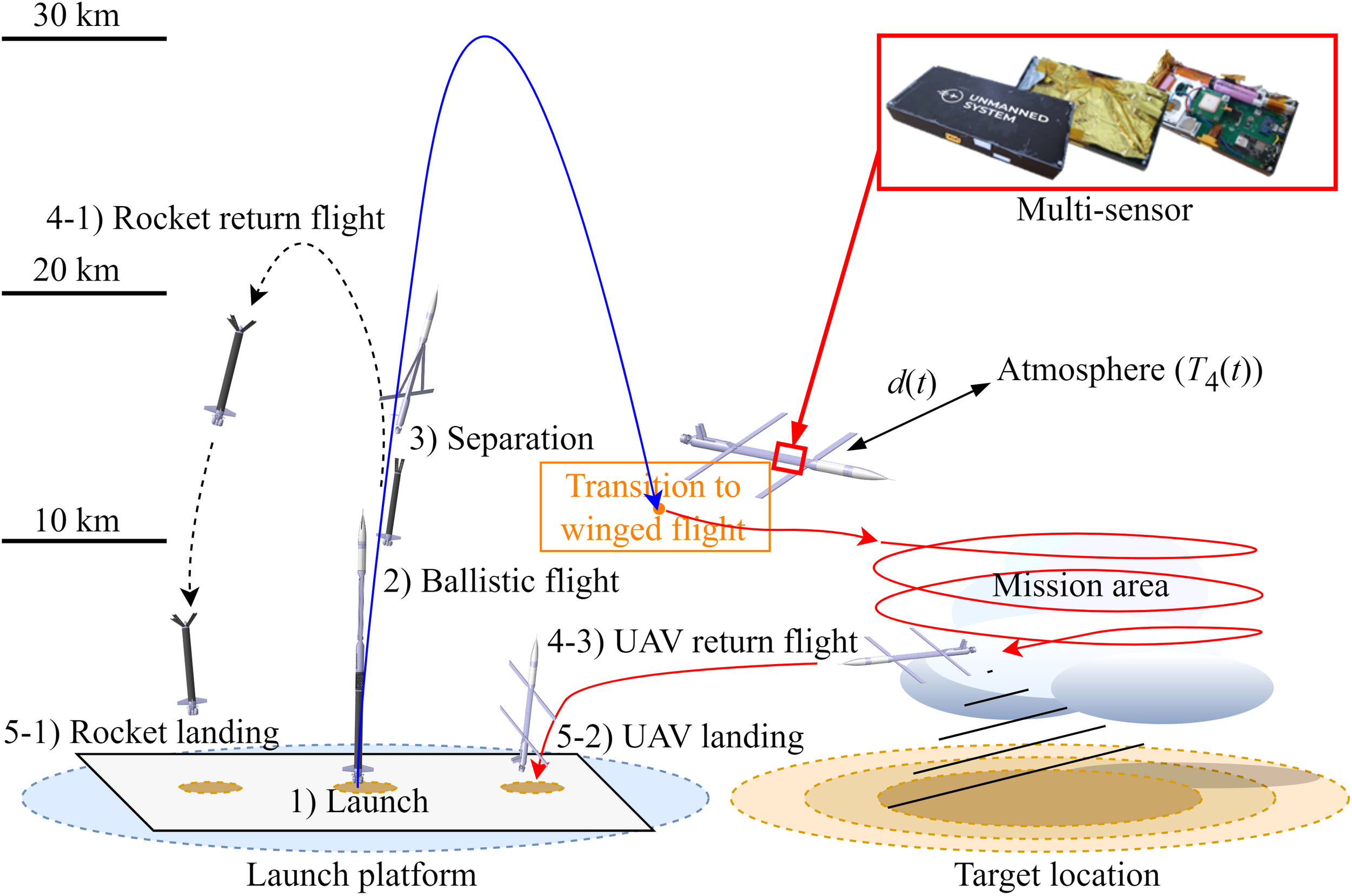
Figure 1. Overview of a UAV-attached multi-sensor mission.

Embedding a disturbance observer in the sensor MCU allows the payload to infer the thermal and electrical states of both peer sensors and the sensor itself without additional reference hardware. This enables anomaly-aware fusion by withholding inconsistent sensors and supports on-board bias correction of calibration-relevant states, while keeping the system minimal.

1.2 Contributions

The main contributions of this study are as follows.

● We propose a disturbance-aware compensation architecture by embedding a DOB on the sensor MCU. It infers calibration-relevant internal states from existing measurements and compensates them on board, avoiding additional hardware installation for sensor calibration.

● We validate the approach in a thermal-vacuum chamber that reproduces a rapid ground-to-stratosphere ascent and show that corrected measurements remain stable during steep temperature and pressure transients.

● We lay the groundwork for redundancy-aware cross-estimation among co-located identical sensors to identify and exclude inconsistent readings during rapid ambient transients without additional hardware.

● These advances improve the measurement reliability of lightweight, miniaturized sensors on mobile platforms and enable reliable upper-air profiling beyond the reach of fixed stations.

1.3 Organization

The remainder of this paper is organized as follows. Section 2 presents the mathematical models, control architecture, implementation of the DOB, and the sensor-compensation strategy. Section 3 describes the system-identification procedure and parameter estimation, validating the theoretical model with the proposed multi-sensor design. Section 4 outlines the simulation and chamber-test setup, including scenarios and protocols used to evaluate the system under controlled conditions. Section 5 reports the experimental observations, with a linear-regression analysis comparing the estimated temperature against reference measurements. Finally, Section 6 summarizes the conclusions and outlines future research directions.

2 Mathematical modeling

The multi-sensor system was designed to measure environmental and positional information transmitted to the server. This includes devices such as electrochemical gas sensors, batteries, and processors operating within certain temperature ranges. However, the external environment of a multi-sensor system may exceed these operating ranges. Therefore, the temperature control is fundamentally performed by the system. Figure 2 shows an overview of the controller and plant system for the temperature control of a multi-sensor system.

Figure 2

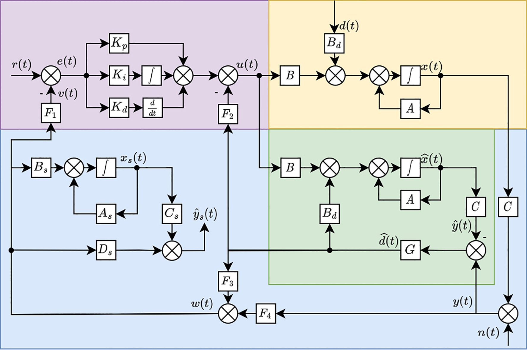
Figure 2. Block diagram of the multi-sensor system.

In this configuration, the plant section represents an unknown model of the system. It was assumed that the controller outputs heat. The role of the DOB is to detect unobserved external temperature variations as well as the heat generation and voltage fluctuations that occur during the operation of processors and communication devices. This observer provides crucial information necessary to compensate for the sensor data.

2.1 Plant

A multi-sensor setup was designed to maintain the operational temperature range of the sensors by adjusting the heater power. It operates as part of a feedback loop, where the controller modifies its output based on the sensor data and system requirements. The following equations describe the general state-space representation of the plant:

$\begin{array}{ll}\begin{array}{l}\dot{x}=Ax+Bu+B_{d}d(t)\\ y(t)=Cx(t)\end{array}& (1)\end{array}$

where $A$ is the state matrix, $B$ is the input matrix, $B_d$ is the disturbance input matrix, $C$ is the output matrix, $d(t)$ is the disturbance, $u(t)$ is the plant input, $x(t)$ is the state vector of the system, and $y(t)$ is the output.

2.2 Disturbance observer

The DOB detects and compensates for disturbances that are not directly observed by sensors, such as temperature variations and voltage fluctuations caused by the operation of processors and communication devices. By providing real-time disturbance compensation, the DOB ensures that the sensor data remain accurate despite external environmental variations. The disturbance $\widehat{d}(t)$ obtained from the DOB was used to adjust the sensor data. This yields the estimated output $\widehat{y}(t)$ of the system after disturbance compensation. The plant model with the estimated disturbance is represented as:

$\begin{array}{ll}\begin{array}{l}\widehat{\dot{x}}=A\widehat{x}+Bu+B_d\widehat{d}(t)\\ \widehat{y}(t)=C\widehat{x}(t)\end{array}& (2)\end{array}$

Assuming that $x(t)=\widehat{x}(t)$, the disturbance $\widehat{d}(t)$ is calculated directly from Equations 1 and 2, as shown in Equation 3:

$\begin{array}{ll}\widehat{d}(t)=B_d^{-1}[\widehat{\dot{x}}-A\widehat{x}-Bu(t)]& (3)\end{array}$

However, this approach assumes that the model effectively matches a real system. Model errors can generate inaccuracies in observed disturbances. The differential equation of the disturbance relative to the estimated disturbance $\widehat{d}(t)$ where defined in the Equation 18 in (Chen et al., 2016) as:

$\begin{array}{ll}\begin{array}{l}\widehat{d}=G_q(s)\tilde{d}(s)\\ \tilde{d}=d-\widehat{d}\end{array}& (4)\end{array}$

where $G_q(s)$ is the Q-filter that substitutes for the products of $B_d$ and $C$ accounting for model uncertainty. Thus, if estimation fast enough $\tilde{x}\approx 0$, by estimating the state disturbance using Equations 1, 2 and 4, we obtain as shown in Equation 5:

$\begin{array}{ll}\widehat{\dot{d}}=G(s)(y-\widehat{y})& (5)\end{array}$

where $\widehat{y}(t)$ is the observed output from (2) and $y(t)$ is the system output measured directly by the sensors, and $G(s)$ is the high-pass filter as a matrix-valued transfer function designed to ensure that $\tilde{d}(t)$ converges to zero.

2.3 Sensor estimator

To accurately predict the sensor output $y_s(t)$, it is important to measure the state of the sensor. Therefore, estimating the state $x_s(t)$ of the sensor and calculating an accurate measurement can be expressed as:

$\begin{array}{ll}\begin{array}{l}{\dot{x}}_s(t)=A_s{x}_s(t)+B_{s}w(t)\\ {\widehat{y}}_s(t)=C_s{\widehat{x}}_s(t)+D_s\widehat{w}(t)\end{array}& (6)\end{array}$

where $A_s$ represents the state-transition matrix of the sensors, $B_s$ is the input matrix of the sensors affected by the sensor input $w(t)$, $C_s$ is the output matrix of the sensors, and $D_s$ is the feed-through of the sensors. The estimated sensor input $\widehat{w}(t)$ is defined as shown in Equation 7:

$\begin{array}{ll}\widehat{w}(t)=F_3\widehat{d}(t)+F_{4}y(t)& (7)\end{array}$

where $F_3$ and $F_4$ are the matrices designed for the sensor estimation from and $\widehat{d}(t)$, $y(t)$ respectively. The sensors measured $y(t)$ with a measurement noise $n(t)$.

2.4 Controller

The system controller plays a crucial role in maintaining the operational stability of the sensors by controlling their temperature. The heating elements in the system were dynamically adjusted to maintain the desired temperature range. This is essential for accurate data collection under dynamic environmental conditions. Proactive temperature management helps mitigate the effects of rapid temperature variations owing to external factors such as UAV operations.

To optimize the control and minimize the energy consumption, the controller uses the reference input $r(t)\in [T_0(t),\dots ,T_i(t)]$. This is the set of target temperatures. Here, each $T_i(t)$ corresponds to a specific $i^{th}$ component within the system. The general proportional-integral-derivative controller can be expressed as shown in Equation 8:

$\begin{array}{ll}\dot{c}(t)=K_d\ddot{e}(t)+K_p\dot{e}(t)+K_{i}e(t)& (8)\end{array}$

where $c(t)\in [{\dot{Q}}_0(t),\dots ,{\dot{Q}}_i(t)]$, ${\dot{Q}}_i(t)$, represents the designed controllable heat generation in each $i^{th}$ element, $e(t)$ represents the control error, and controllers gain matrix $K_p$, $K_i$, and $K_d$ are designed to $e(\infty )=0$. In Equation 9, e(t) and v(t) are defined as:

$\begin{array}{ll}\begin{array}{l}e(t)=r(t)-v(t)\\ v(t)=F_{1}w(t)\end{array}& (9)\end{array}$

where F₁ is the matrix designed for controller from $w(t)$.

Finally, the controller output $u(t)$ is defined in Equation 10:

$\begin{array}{ll}u(t)=c(t)-F_2\widehat{d}(t)& (10)\end{array}$

where $F_2$ is a matrix designed to compensate for $\widehat{d}(t)$ in $u(t)$. The integration of this control mechanism with sensors ensured that each component operated within its threshold. This enhances the overall robustness and reliability of the system. The following sections discuss the advanced functionalities and integration of the DOB and sensors within this refined control framework.

3 System identification and parameter estimation

To validate the proposed method under real-world conditions, it was applied to a multi-sensor system mounted on a UAV for atmospheric observations. This system was used for identification and parameter estimation. The specifications are listed in Table 2.

Table 2

Table 2. Specifications of the multi-sensor.

The multi-sensor system transmitted and received positional information and data from external sources through satellite communication (SATCOM), long-term evolution (LTE), ultra-wideband (UWB), and global positioning system (GPS) modules. In addition, it controls the heat generated by the integrated heater. Various types of gases, particulate matter, temperature, and humidity sensors have been used to acquire environmental data. The goal of the validation was to predict the atmospheric temperature using the proposed DOB-based sensor estimation method and compare it with a reference atmospheric temperature sensor. This approach is important because it can be used to predict the external and internal sensor temperatures, which are crucial because most chemical sensors are vulnerable to temperature variations.

3.1 Model

A mathematical model was required to apply the DOB, based on which we developed a mobile multi sensor system and temperature model. Figure 3 illustrates the multi-sensor system and its components. This figure shows the temperature states of the $i^{th}$ component, denoted as $T_i(t)$. For the identification, we define the output matrix $C$, state $x(t)$, and sensor output $y_s(t)$ as follows:

Figure 3

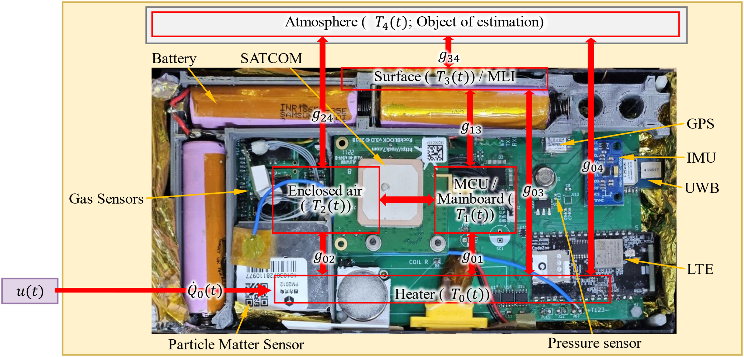
Figure 3. Multi-sensor model overview.

$\begin{array}{ll}\begin{array}{l}C=\left[\begin{array}{cccc}1& 0& 0& 0\\ 0& 1& 0& 0\\ 0& 0& 1& 0\\ 0& 0& 0& 1\end{array}\right]\\ x(t)=[T_0(t)T_1(t)T_2(t)T_3(t)]\\ y_s(t)=T_4(t)\end{array}& (11)\end{array}$

where $i\in [0,1,2,3,4]$ represents the heater, microcontroller unit with the mainboard, enclosed air within the multi-sensor, surface temperature outside the multi-layered insulation (MLI), and atmosphere, respectively. Although the atmosphere is not a component of a multi-sensor system, it is expressed as the fourth component to derive the equations. Each of $T_0(t)-T_3(t)$ were measured using dedicated temperature sensors. However, no sensor was installed to measure the atmospheric temperature $T_4$ in the multi-sensor system. In this system, $u(t)$ and $d(t)$ are defined as the heat transfer between each component 208 and the atmosphere. These are expressed as follows:

$\begin{array}{ll}\begin{array}{l}u(t)={\dot{Q}}_c(t)-{\dot{Q}}_{04}(t)={\dot{Q}}_0(t)\\ d(t)={[{\dot{Q}}_{04}(t){\dot{Q}}_{14}(t){\dot{Q}}_{24}(t){\dot{Q}}_{34}(t)]}^T\end{array}& (12)\end{array}$

where ${\dot{Q}}_c(t)$ represents the electric heater power.

The total heat transfer rate.

${\dot{Q}}_i(t)$ for each component can be expressed in terms of the heat capacity and 211 heat transfer between i and j as follows:

$\begin{array}{ll}\begin{array}{l}{\dot{Q}}_i(t)={\dot{T}}_i(t)c_i,\\ {\dot{Q}}_i(t)=\sum _{j=0}^4{\dot{Q}}_{ij}(t)\end{array}& (13)\end{array}$

where $c_i$ is the heat capacity of the $i^{th}$ component. ${\dot{Q}}_{ij}(t)$ is the heat-transfer rate between components $i$ and $j$, as follows:

$\begin{array}{ll}{\dot{Q}}_{ij}(t)=g_{ij}(T_i(t)-T_j(t))& (14)\end{array}$

where $g_{ij}$ [W/K] represents the thermal conductance.

From Equations 13 and 14, the differential equation of the plant model is expressed as.

$\begin{array}{ll}{\dot{T}}_i(t)=c_i^{-1}\left(\sum _{j=0}^3{g}_{ij}(T_i(t)-T_j(t))+{\dot{Q}}_{i4}(t)\right)& (15)\end{array}$

The relationships between $Q_{ij}(t)$ and $Q_{ji}(t)$, $g_{ij}(t)$ and $g_{ji}(t)$, and the self-heat transfer terms ${\dot{Q}}_{ii}$ and $g_{ii}$are expressed as follows:

$\begin{array}{ll}\begin{array}{l}{\dot{Q}}_{ij}(t)=-{\dot{Q}}_{ji}(t), {\dot{Q}}_{ii}(t)=0,\\ g_{ij}=-g_{ji}, g_{ii}=0\end{array}& (16)\end{array}$

From Equations 11, 12, 15 and 16, we obtain the following temperature ODEs:

$\begin{array}{ll}\begin{array}{l}{\dot{T}}_0(t)=c_0^{-1}\left({\dot{Q}}_{04}(t)+g_0{T}_0(t)-g_{01}{T}_1(t)-g_{02}{T}_2(t)-g_{03}{T}_3(t)\right)\\ {\dot{T}}_1(t)=c_1^{-1}\left({\dot{Q}}_{14}(t)+g_1{T}_1(t)+g_{01}{T}_0(t)-g_{12}{T}_2(t)-g_{13}{T}_3(t)\right)\\ {\dot{T}}_2(t)=c_2^{-1}\left({\dot{Q}}_{24}(t)+g_2{T}_2(t)+g_{02}{T}_0(t)+g_{12}{T}_2(t)-g_{23}{T}_3(t)\right)\\ {\dot{T}}_3(t)=c_3^{-1}\left({\dot{Q}}_{34}(t)+g_3{T}_3(t)+g_{03}{T}_0(t)+g_{13}{T}_1(t)+g_{23}{T}_2(t)\right)\\ \text{where\hspace{1em}}{g}_0=g_{01}+g_{02}+g_{03},g_1=-g_{01}+g_{12}+g_{13},\\ g_2=-g_{02}-g_{12}+g_{23},g_3=-g_{03}-g_{13}-g_{23}\end{array}& (17)\end{array}$

These equations can be compactly expressed in state-space form as.

$\begin{array}{ll}\begin{array}{l}A=\left[\begin{array}{l}\begin{array}{cccc}{c}_0^{-1}{g}_0& -c_0^{-1}{g}_{01}& -c_0^{-1}{g}_{02}& -c_0^{-1}{g}_{03}\end{array}\\ \begin{array}{cccc}{c}_1^{-1}{g}_{01}& c_1^{-1}{g}_1& c_1^{-1}{g}_{12}& -c_1^{-1}{g}_{13}\end{array}\\ \begin{array}{cccc}{c}_2^{-1}{g}_{02}& c_2^{-1}{g}_{12}& c_2^{-1}{g}_2& -c_2^{-1}{g}_{23}\end{array}\\ \begin{array}{cccc}{c}_3^{-1}{g}_{03}& c_3^{-1}{g}_{13}& c_3^{-1}{g}_{23}& c_3^{-1}{g}_3\end{array}\end{array}\right],\\ B_d=\left[\begin{array}{cccc}{c}_0^{-1}& 0& 0& 0\\ 0& c_1^{-1}& 0& 0\\ 0& 0& c_2^{-1}& 0\\ 0& 0& 0& c_3^{-1}\end{array}\right],B=\left[\begin{array}{c}{c}_0^{-1}\\ 0\\ 0\\ 0\end{array}\right]\end{array}& (18)\end{array}$

where matrices A, B, and B_d are defined in Equation 18 as the compact state-space representation of Equation 17.

3.2 Disturbance observer

As the gain G of the DOB increased, the rate of decrease in the disturbance error decreased. However, if G is excessively high, the sensor noise may be amplified and the quality of the estimation results may be degraded. We selected a G value that was ten times higher than the sensor data collection frequency (0.25Hz) to balance error reduction and noise amplification in this system.

In addition, the optimal G can be obtained by defining the estimation error at the most rapidly changing point of the linearized model as the cost function and solving it through simulation and experiments using a sequential quadratic programming (SQP) algorithm. In this study, we employed the optimization results derived from both the external temperature simulation and the experimental data described in Section 4. The optimized G for this model is constant, consistent with the state estimation framework, and all experiments were conducted under identical conditions.

3.3 Sensor estimator

The DOB-based sensor estimator predicts the states of sensors that cannot be measured directly. In this study, a virtual atmospheric temperature sensor was designed to verify the performance of the sensor estimator. Assuming a multi-sensor without an external conductive medium, all thermal disturbances originate externally. From Equations 13, 14 and 16, we obtain as shown in Equation 19:

$\begin{array}{ll}\sum _{i=1}^4{Q}_i(t)=\sum _{i=1}^4{Q}_{i4}(t)& (19)\end{array}$

Thus, the estimated sensor output ${\widehat{y}}_s(t)$ from Equation 6 where designed:

$\begin{array}{ll}\begin{array}{l}{\widehat{y}}_s(t)=D_{s}w(t)\\ D_s=[aaaab{g}_{04}b{g}_{14}b{g}_{24}b{g}_{34}]\\ a=0.25,b={({\displaystyle \sum _{i=0}^3}{g}_{i4})}^{-1}\end{array}& (20)\end{array}$

where the sensor model input vector w(t) in Equation 20 is defined as:

$\begin{array}{ll}w(t)=\left[\begin{array}{c}\widehat{d}(t)\\ y(t)\end{array}\right]& (21)\end{array}$

Therefore, from Equation 21 and the block diagram in Figure 2, the designed matrices F₃ and F₄ are defined in Equation 22.

$\begin{array}{ll}\begin{array}{l}{F}_3=\left[\begin{array}{cccccccc}1& 0& 0& 0& 0& 0& 0& 0\\ 0& 1& 0& 0& 0& 0& 0& 0\\ 0& 0& 1& 0& 0& 0& 0& 0\\ 0& 0& 0& 1& 0& 0& 0& 0\end{array}\right]F_4=\left[\begin{array}{cccccccc}0& 0& 0& 0& 1& 0& 0& 0\\ 0& 0& 0& 0& 0& 1& 0& 0\\ 0& 0& 0& 0& 0& 0& 1& 0\\ 0& 0& 0& 0& 0& 0& 0& 1\end{array}\right]\end{array}& (22)\end{array}$

3.4 Parameter estimation

Parameter estimation was performed to determine the thermal conductance and heat capacity of the system. Although some thermal conductance g_ij and heat capacity c_i values can vary with atmospheric pressure, in this study, we assumed a constant linear system, considering that the DOB was designed to operate even with model uncertainties. The trust-region-reflective least-squares algorithm is commonly used for nonlinear optimization. This was employed for the estimation. The parameters obtained through the optimization process are listed in Table 3.

Table 3

Table 3. List of estimated parameters.

The simulation process was based on a point-mass model capable of simulating nonlinear variations in the drag and mass. Using the mission settings specified in Table 4, we simulated the UAV trajectories as shown in Figure 4.

Table 4

Table 4. Scenario configurations for UAV missions.

Figure 4

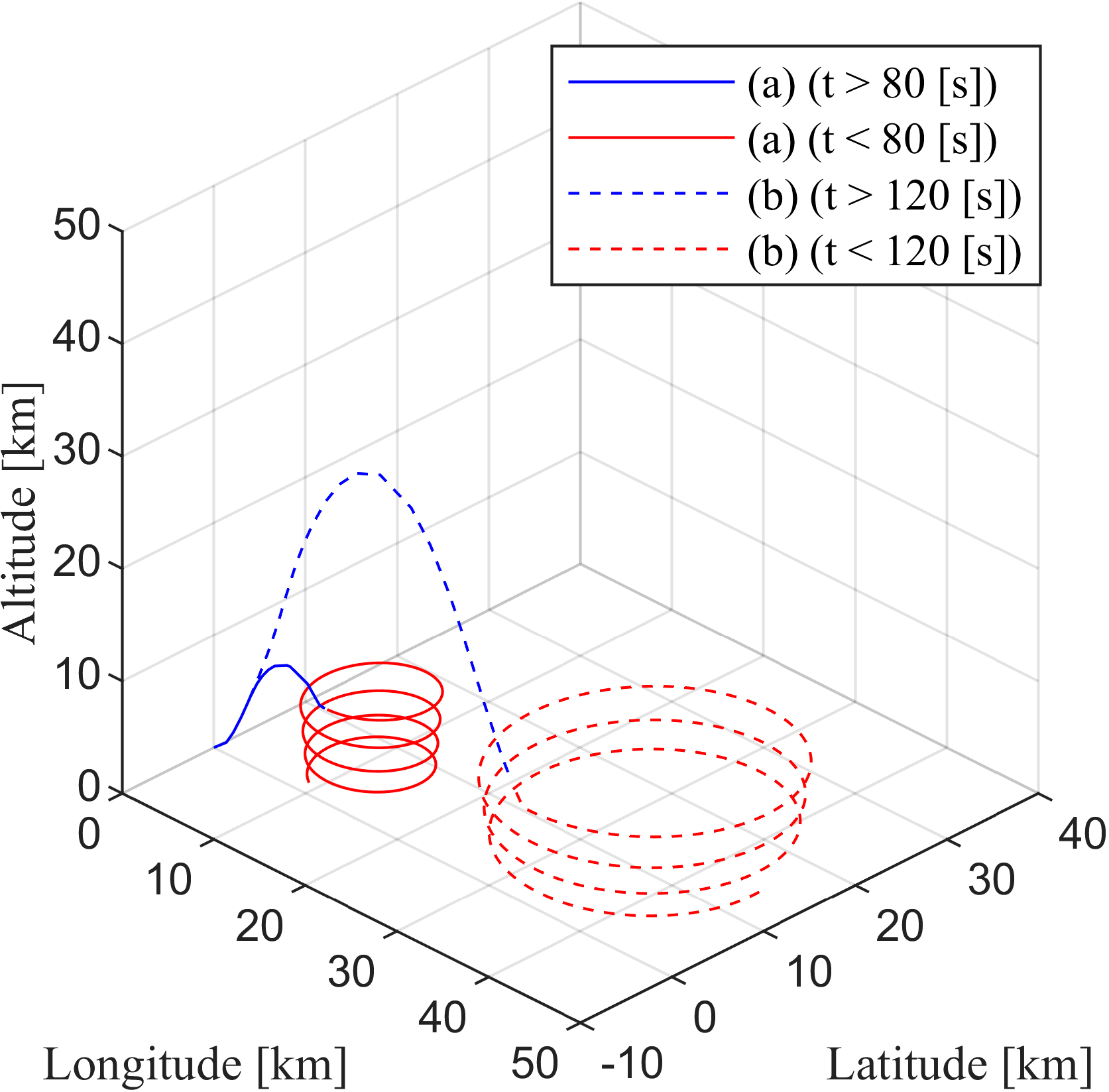
Figure 4. AV trajectories. Legend labels (a) and (b) denote Scenario I and II, respectively.

4 Simulation and experiment

4.1 Simulation

To evaluate the proposed system, we established a series of real mission scenarios for the multi-sensor system, simulating temperature and pressure conditions. The UAV-attached sensor rapidly increases to its maximum altitude via rocket propulsion. After attaining the maximum altitude, the UAV deploys its wings and transitions to gliding after it attains the winged flight altitude. This continues until the ballistic flight time ends and then decreases during the total flight time. Each scenario varied in terms of the maximum altitude attained and descent speed. The results are listed in Table 4.

Using the mission settings specified in Table 4, we simulated the UAV trajectories as shown in Figure 4. The trajectories were generated with a point-mass profile generator capable of simulating nonlinear variations in drag and mass, implemented within a MATLAB/Simulink based simulation model reused from our prior works. The dynamic model comprises a 6-DOF ECEF rigid-body with gravity, ground, mass, wind/atmosphere (ISA), and NED model based controller blocks; propulsion and airframe submodels for rocket booster ascent and turbojet/UAV flight with aerodynamics; and actuator subsystems for servo and gimbal. We did not modify the governing equations for this study and only adjusted the scenario parameters to match Table 4. Full details of the simulation and settings are provided in Kim et al (2024, 2025).

Using the international standard atmosphere model, we converted the altitude variations over time into corresponding temperature and pressure variations, as illustrated in Figure 5. The temperature and pressure data for each scenario derived from these simulations served as the basis for setting the conditions for the subsequent experiments, enabling rigorous and realistic performance testing of the sensor system.

Figure 5

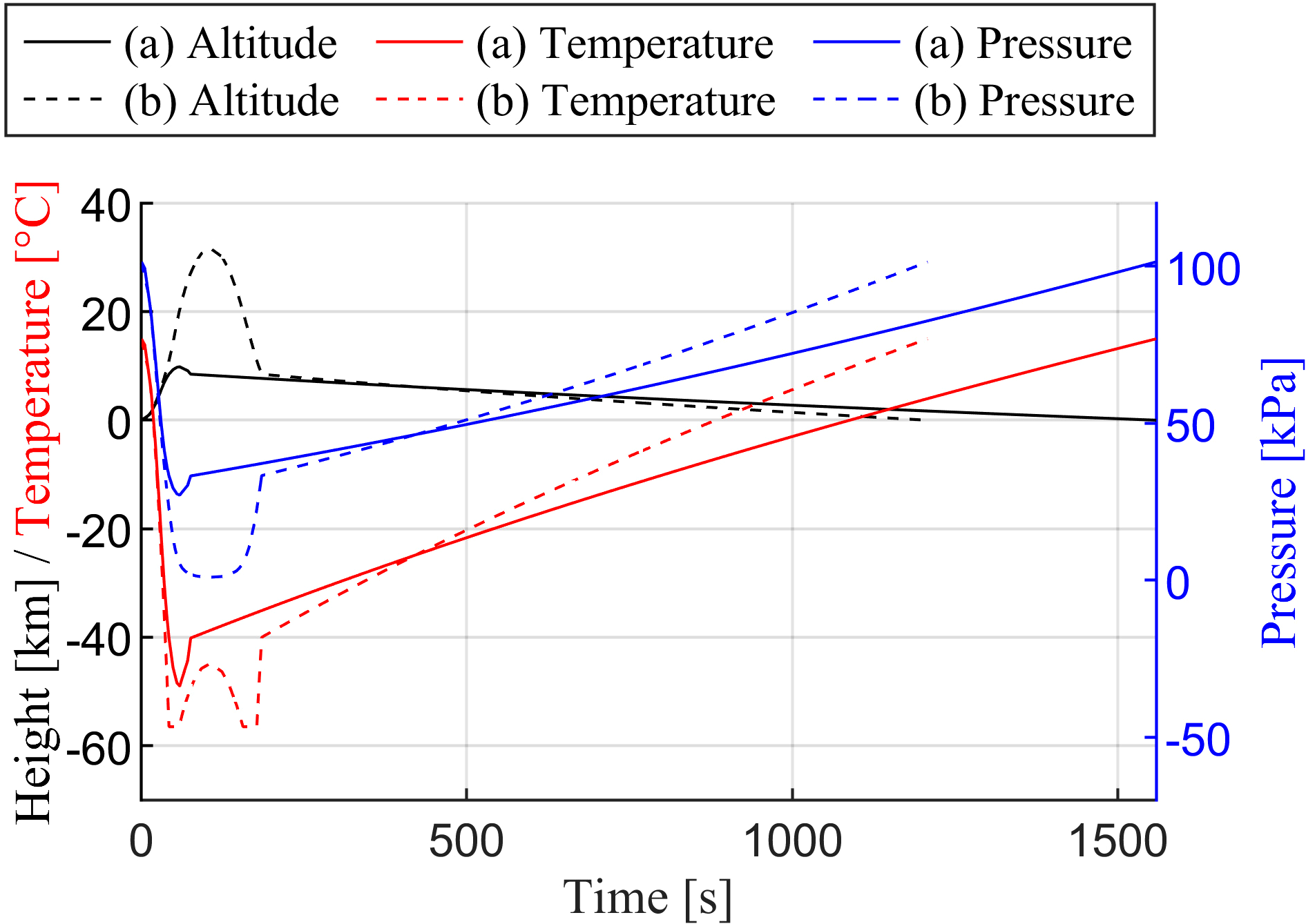
Figure 5. Simulation results. Legend labels (a) and (b) denote Scenario I and II, respectively.

4.2 Experiment

We conducted experiments according to these steps to accurately implement the temperature and pressure variations set by the simulation and compared them with those of the reference sensor. We used the given (a) scenario I and (b) scenario II to set up the experimental environment by utilizing the high-altitude test chamber configured in Figure 6. Temperature and pressure were controlled in a vacuum chamber.

Figure 6

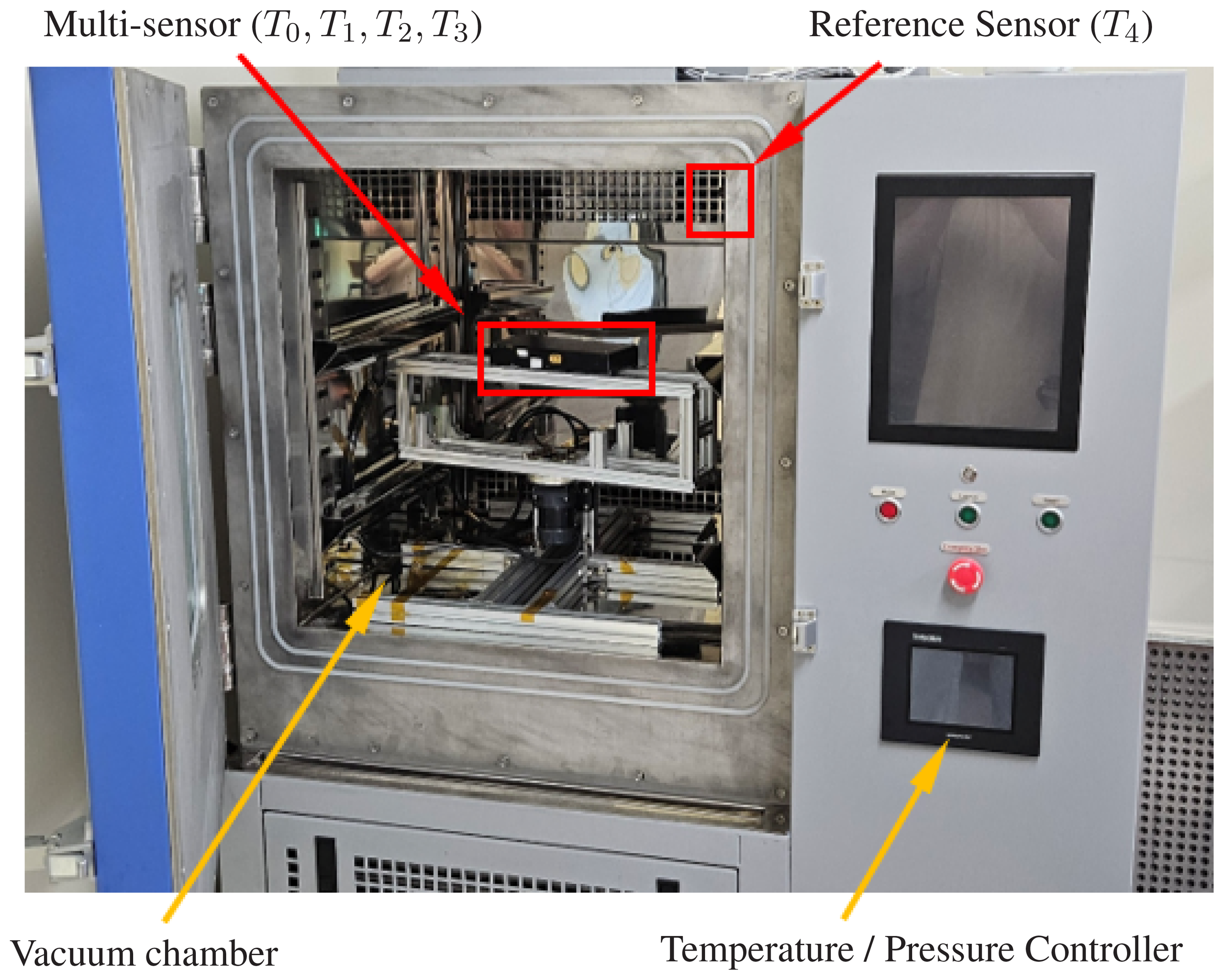
Figure 6. Experimental configuration.

However, owing to the limitations of the experimental apparatus, the accurate replication of the experimental environment is challenging. Therefore, the scenarios were restructured as follows: Test I, Test II, and Test III to adjust the time required to attain the target temperature. Each test followed the step-by-step target temperature and pressure of the underlying scenario, although marginally different times were required to attain the targets.

The experiments were performed three times to detect the disturbances caused by internal heat generation and compare the performance of the sensor estimator. Specifically, in Test III, arbitrary disturbances were introduced to include temperature variations from the internal heater, external temperature variations, and pressure variations derived from a modification of Test I. The resulting variations in temperature, pressure, and heater operation ${\dot{Q}}_o(t)$in Test III are detailed in the Results and Evaluation section.

The experimental setup included a shelf for mounting the multi-sensor and a reference sensor that measured atmospheric temperature. According to the simulation, the temperature and pressure varied from over 20°C to −40°C and from 100kPa to 20kPa within 1min. The chamber was cooled to the target temperature and experiments were conducted after installing the multi-sensor. This is illustrated in Figure 7. These adjustments caused differences in the target temperature, pressure, and timing compared with the original scenario. However, these variations can be detected by a DOB, which is designed to detect abrupt variations in the environment. This highlights the accuracy of sensor estimation and demonstrates the robustness of the system.

Figure 7

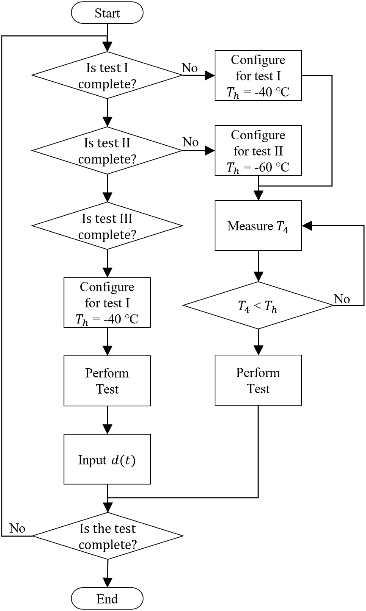
Figure 7. Experimental process flowchart.

5 Results and discussion

We evaluate the approach in a thermal-vacuum chamber that replicates rapid ground-to-stratosphere transients (Section 4).

The experimental setup involved monitoring the internal temperature variations within the multi-sensor using T₃(t) (a temperature sensor mounted on the internal surface) and the atmospheric temperature using T₄(t) (an external reference sensor). The test results, including the pressure variations, are shown graphically in Figures 8a, c, e. Using the collected data, the estimated sensor output ${\widehat{y}}_s(t)$ and the measured temperatures T₃(t) and T₄(t) were compared, as shown in Figures 8b, d, f. To evaluate the accuracy of the estimated temperatures, T₃(t) was selected to represent the atmospheric temperature and it was compared with the reference value T₄(t) and the estimated sensor output ${\widehat{y}}_s(t)$. This is illustrated in Figure 9.

Figure 8

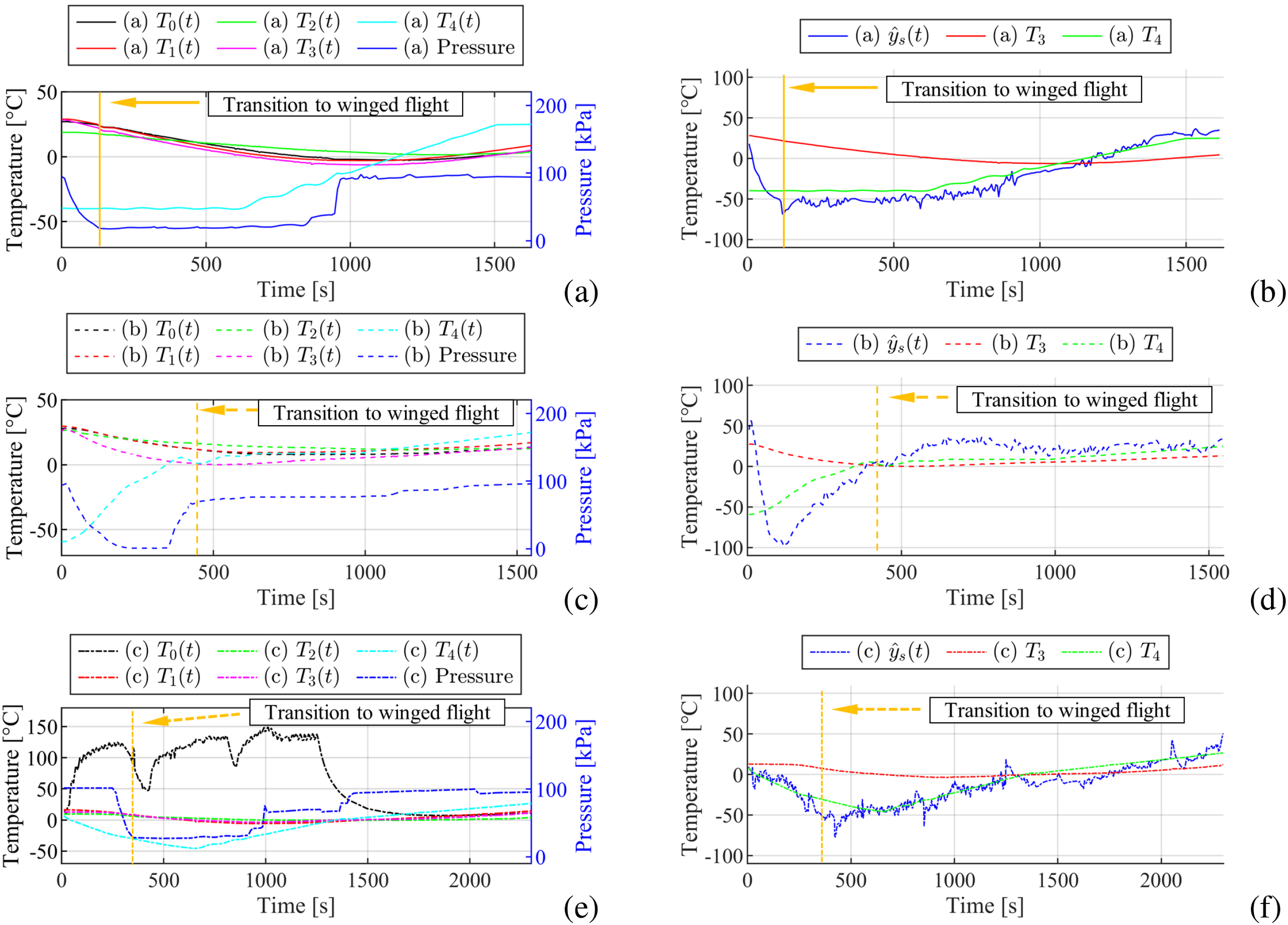
Figure 8. Experimental results: (a) Test I, (c) Test II, (e) Test III; atmospheric-temperature estimates versus sensor readings: (b) Test I, (d) Test II, (f) Test III.

Figure 9

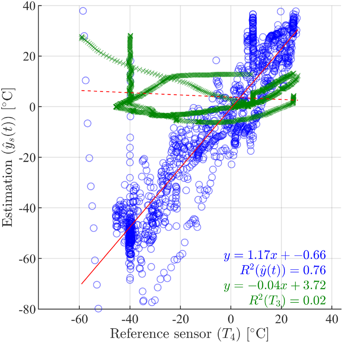
Figure 9. Comparative analysis of the reference and estimation result.

The experimental results and linear-regression analyses demonstrate that the DOB approach can greatly improve the accuracy of atmospheric-temperature estimation when using a surface-mounted sensor. When only the surface-mounted sensor T₃(t) was used, the estimation produced an R² of 0.02, showing a weak correlation with the reference T₄(t). This finding highlights the inadequacy of relying on T₃(t) alone for accurate temperature measurement. After the DOB was incorporated, the R² improved to 0.76, indicating increased correlation between the estimated and actual atmospheric temperatures, as high R² values have been shown to reflect good sensor performance (Yeom, 2021). The regression coefficient likewise increased from -0.04 to 1.17, confirming that the estimation shifted from a statistically non-significant to a significant level.

To illustrate the performance improvements, Table 5 presents a detailed comparison of the measurement and estimation errors for Test I-III together with their average (AVG) values. It presents the maximum error (MAX), mean error (MEAN), minimum error (MIN), and root mean square error (RMSE) calculated for errors ${\tilde{T}}_3$ and ${\widehat{y}}_s(t)$, which are the differences between T₃(t), ${\widehat{y}}_s(t)$ and the reference T₄(t), respectively. Errors ${\tilde{T}}_{3,z}$and ${\tilde{T}}_{s,z}$occur at each time step z and are defined in Equation 23:

Table 5

Table 5. Measurement and estimation errors (all values in °C).

$\begin{array}{ll}\begin{array}{l}{\tilde{T}}_{3,z}=T_{4,z}-T_{3,z}\\ {\tilde{y}}_{s,z}=T_{4,z}-{\widehat{y}}_{s,z}\end{array}& (23)\end{array}$

The errors are calculated in Equation 24 as follows:

$\begin{array}{ll}\begin{array}{l}MAX=max(e_z)MEAN=\frac{1}{l}\sum _{z=1}^l{e}_z\\ MIN=min(e_z)RMSE=\sqrt{\frac{1}{l}{\displaystyle \sum _{z=1}^l}{e}_z^2}\end{array}& (24)\end{array}$

where $e_z\in [{\tilde{T}}_{3,z},{\tilde{y}}_{s,z}]$ represents the error and $l$ is the total number of data points.

RMSE is a critical indicator of the estimation accuracy. It improved significantly from 28.67 for ${\tilde{T}}_3$ to 15.76 for ${\tilde{y}}_s(t)$. This significant reduction in RMSE emphasizes the efficacy of the DOB with the sensor estimator in providing more precise temperature readings. Further analysis of the error metrics revealed that MAX, MEAN, and MIN improved significantly. For example, the average mean error for ${\tilde{T}}_3$ was -13.24, whereas it reduced significantly to 1.76 for ${\tilde{y}}_s$. However, the maximum error average increased from 16.80°C to 43.26°C, and the minimum error average improved from −66.72°C to −66.02°C. The improvements in MAX and MIN were smaller than those in the other two metrics. This phenomenon can be attributed to the setting of the initial state variables of the observer to zero. As shown in Figure 8f, where the initial temperature T₄(0) is near zero, the MAX and MIN values are closer to zero than those in Figures 8b, d, where the T₄(0) values are below −40°C.

For reference, all nomenclature and estimated values used in this paper are listed in Table 6.

Table 6

Table 6. List of nomenclatures.

6 Conclusion

In this study, we presented a novel approach for enhancing the sensor accuracy in mobile multi-sensor systems for atmospheric monitoring. By integrating the DOB with sensor estimators, we demonstrated accurate atmospheric temperature prediction using only temperature sensors. This validation was achieved through rigorous experiments utilizing a DOB to compensate for internal and external disturbances. The experimental results revealed that the R² value significantly improved from 0.02 to 0.76 with the DOB and sensor estimators, indicating a substantial enhancement in prediction accuracy. These values are comparable to those reported for prior methods summarized in Table 1, indicating a correlation sufficient for practical use of the estimated temperature. Excluding cases where the reference sensor is co-located within the same vehicle, this performance is broadly comparable to typical estimation results reported in the literature. Considering the rapid external temperature transients and the ultralight, low-cost sensor suite used here, the result is particularly encouraging for mobile platform deployments.

Beyond temperature, the same disturbance-aware architecture can be extended to humidity, particulate-matter, and trace-gas sensors, providing a pathway toward fully compensated multi-parameter payloads for high-resolution air-sea flux studies. Because the method operates on-board and requires no external calibration hardware, it is well suited to the strict mass-and-power budgets of small UAVs and other mobile platforms.

An additional consideration is sensor corruption or failure. While the present study intentionally focused on redundancy-free operation to establish a baseline, when multiple co-located sensors are available, cross-estimation among them can be used to flag abnormal readings and maintain robustness. With n sensors, there are 2ⁿ − 2 valid subsets of the remaining sensors (excluding the empty set and the full set). For each subset, the sensor-estimation method presented in this study can be applied to generate an independent cross-estimate of the target sensor, and statistical comparison with the actual measurement enables the detection of persistent anomalies. Within the chamber setting reported here, random noise and sporadic dropouts are already mitigated by the DOB itself, while persistent bias would require such redundancy-based cross-estimation. Practical implementations could further combine covariance-based residual checks with a simple decision layer to exclude a suspected sensor and preserve reliable operation. This positions the present work as a foundation for future extensions toward redundancy-aware sensing frameworks.

Future work will focus on flight campaigns over coastal and open-ocean regions. These missions will validate the payload under real atmospheric dynamics, assess long-term stability, and explore the integration of additional sensing channels. Ultimately, we expect that disturbance-aware profiling systems will expand the spatial reach and data quality of coupled atmosphere-ocean observations, supporting both scientific research and operational environmental monitoring.

Data availability statement

The original contributions presented in the study are included in the article/supplementary material. Further inquiries can be directed to the corresponding author.

Author contributions

SK: Conceptualization, Writing – original draft, Writing – review & editing. AT: Writing – review & editing. SJ: Funding acquisition, Supervision, Writing – review & editing.

Funding

The author(s) declare financial support was received for the research and/or publication of this article. This work was supported by Korea Institute for Advancement of Technology (KIAT) grant funded by the Korea Government (MOTIE) (P0024180, Development of RIC (Regional Innovation Cluster)).

Conflict of interest

The authors declare that the research was conducted in the absence of any commercial or financial relationships that could be construed as a potential conflict of interest.

Generative AI statement

The author(s) declare that no Generative AI was used in the creation of this manuscript.

Any alternative text (alt text) provided alongside figures in this article has been generated by Frontiers with the support of artificial intelligence and reasonable efforts have been made to ensure accuracy, including review by the authors wherever possible. If you identify any issues, please contact us.

Publisher’s note

All claims expressed in this article are solely those of the authors and do not necessarily represent those of their affiliated organizations, or those of the publisher, the editors and the reviewers. Any product that may be evaluated in this article, or claim that may be made by its manufacturer, is not guaranteed or endorsed by the publisher.

Abbreviations

DOB, disturbance observer; UAV, unmanned aerial vehicle; GPS, global positioning system; IoT, internet of things; LTE, long-term evolution; SATCOM, satellite communication; UWB, ultra-wideband; RMSE, root mean square error; AVG, average; MAX, maximum error; MEAN, mean error; MIN, minimum error; PM, particulate matter.

References

Ali S., Glass T., Parr B., Potgieter J., and Alam F. (2021). Low cost sensor with iot lorawan connectivity and machine learning-based calibration for air pollution monitoring. IEEE Trans. Instrumentation Measurement 70, 1–11. doi: 10.1109/tim.2020.3034109

Crossref Full Text | Google Scholar

Allka X., Ferrer-Cid P., Barcelo-Ordinas J. M., and Garcia-Vidal J. (2023). Temporal pattern-based denoising and calibration for low-cost sensors in iot monitoring platforms. IEEE Trans. Instrumentation Measurement 72, 1–11. doi: 10.1109/tim.2023.3239626

Crossref Full Text | Google Scholar

Chen W.-H., Yang J., Guo L., and Li S. (2016). Disturbance-observer-based control and related methods—an overview. IEEE Trans. Ind. Electron. 63, 1083–1095. doi: 10.1109/tie.2015.2478397

Crossref Full Text | Google Scholar

Chen Z., Zhang T., Chen Z., Xiang Y., Xuan Q., and Dick R. P. (2021). Hvaq: A high-resolution vision-based air quality dataset. IEEE Trans. Instrumentation Measurement 70, 1–10. doi: 10.1109/tim.2021.3104415

Crossref Full Text | Google Scholar

Concas F., Mineraud J., Lagerspetz E., Varjonen S., Liu X., Puolamäki K., et al. (2021). Low-cost outdoor air quality monitoring and sensor calibration: A survey and critical analysis. ACM Trans. Sensor Networks 17, 1–44. doi: 10.1145/3446005

Crossref Full Text | Google Scholar

Daoud S., Mdhaffar A., Jmaiel M., and Freisleben B. (2020). Q-rank: Reinforcement learning for recommending algorithms to predict drug sensitivity to cancer therapy. IEEE J. Biomed. Health Inf. 24, 3154–3161. doi: 10.1109/jbhi.2020.3004663

PubMed Abstract | Crossref Full Text | Google Scholar

Fekih M. A., Bechkit W., Rivano H., Dahan M., Renard F., Alonso L., et al. (2021). Participatory air quality and urban heat islands monitoring system. IEEE Trans. Instrumentation Measurement 70, 1–14. doi: 10.1109/tim.2020.3034987

Crossref Full Text | Google Scholar

Gu J., Liu C., Zhuang Y., Du X., Zhuang F., Ying H., et al. (2020). Dynamic measurement and data calibration for aerial mobile iot. IEEE Internet Things J. 7, 5210–5219. doi: 10.1109/jiot.2020.2977910

Crossref Full Text | Google Scholar

Günther M., Schmidt H., Timmreck C., and Toohey M. (2024). Why does stratospheric aerosol forcing strongly cool the warm pool? Atmospheric Chem. Phys. 24, 7203–7225. doi: 10.5194/411acp-24-7203-2024

Crossref Full Text | Google Scholar

Hayward I., Martin N. A., Ferracci V., Kazemimanesh M., and Kumar P. (2024). Low-cost air quality sensors: Biases, corrections and challenges in their comparability. Atmosphere 15, 1523. doi: 10.3390/atmos15121523

Crossref Full Text | Google Scholar

Iwata H., Ohishi K., Yokokura Y., Okada Y., Ide Y., Kuraishi D., et al. (2020). Robust estimation method for stator temperature based on voltage disturbance observer autotuning resistance for spmsm. IEEJ J. Industry Appl. 9, 341–350. doi: 10.1541/ieejjia.9.341

Crossref Full Text | Google Scholar

Kim S., Molla T., Zegeye A., and Jung S. (2025). Energy-efficient control system for small-scale rocket recovery. IEEE Access 13, 104521–104537. doi: 10.1109/access.2025.3579590

Crossref Full Text | Google Scholar

Kim S., Woldeyohannis A. Z., Molla G. T., Kim M., Park E.-J., and Jung S. (2024). “Fuel efficiency analysis of the jet engine and solid-propellant based small reusable sub-orbital launch vehicle candidates,” in IAF Space Transportation Solutions and Innovations Symposium, vol. 2024. (International Astronautical Federation (IAF), 790–797. doi: 10.52202/078373-0082

Crossref Full Text | Google Scholar

Liang L. (2021). Calibrating low-cost sensors for ambient air monitoring: Techniques, trends, and challenges. Environ. Res. 197, 111163. doi: 10.1016/j.envres.2021.111163

PubMed Abstract | Crossref Full Text | Google Scholar

Liu G., Liu Y., Li Z., Ma Z., Ma X., Wang X., et al. (2023). Combined temperature compensation method for closed-loop microelectromechanical system capacitive accelerometer. Micromachines 14, 1623. doi: 10.3390/mi14081623

PubMed Abstract | Crossref Full Text | Google Scholar

Lundstrom H. and Mattsson M. (2020). Radiation influence on indoor air temperature sensors: Experimental evaluation of measurement errors and improvement methods. Exp. Thermal Fluid Sci 115, 110082. doi: 10.1016/j.expthermflusci.2020.110082

Crossref Full Text | Google Scholar

Messier P., Nguyen B.-H., LeBel F.-A., and Trovao J. P. F. (2020). Disturbance observer-based state-of charge estimation for li-ion battery used in light electric vehicles. J. Energy Storage 27, 101144. doi: 10.1016/j.est.2019.101144

Crossref Full Text | Google Scholar

Nadzir M. S. M., Rabuan U., Ali S. H. M., Borah J., Majumdar S., and Rohmad M. S. (2025). Drone-based air quality monitoring: Development and evaluation of low-cost pm2.5 sensor for remote environmental assessment. Sensors Materials 37, 2153. doi: 10.18494/sam5449

Crossref Full Text | Google Scholar

Pohorsky R., Baccarini A., Tolu J., Winkel L. H. E., and Schmale J. (2024). Modular multiplatform compatible air measurement system (momucams): a new modular platform for boundary layer aerosol and trace gas vertical measurements in extreme environments. Atmospheric Measurement Techniques 17, 731–754. doi: 10.5194/amt-17-731-2024

Crossref Full Text | Google Scholar

Saha P. K., Hankey S., Marshall J. D., Robinson A. L., and Presto A. A. (2021). High-spatial-resolution estimates of ultrafine particle concentrations across the continental United States. Environ. Sci Technol. 55, 10320–10331. doi: 10.1021/acs.est.1c03237

PubMed Abstract | Crossref Full Text | Google Scholar

Santina C. D., Truby R. L., and Rus D. (2020). Data-driven disturbance observers for estimating external forces on soft robots. IEEE Robotics Automation Lett. 5, 5717–5724. doi: 10.1109/lra.2020.3010738

Crossref Full Text | Google Scholar

Siddiqui M. A., Baig M. H., and Yousuf M. U. (2025). Performance and data acquisition from low cost air quality sensors: a comprehensive review. Air Quality Atmosphere Health 18, 1183–1203. doi: 10.1007/s11869-024-01683-3

Crossref Full Text | Google Scholar

Tang X. and Xu B. (2023). Reactor temperature compound control strategy based on disturbance observer. IEEE Access 11, 84554–84564. doi: 10.1109/access.2023.3303036

Crossref Full Text | Google Scholar

Wei P., Ning Z., Ye S., Sun L., Yang F., Wong K., et al. (2018). Impact analysis of temperature and humidity conditions on electrochemical sensor response in ambient air quality monitoring. Sensors 18, 59. doi: 10.3390/s18020059

PubMed Abstract | Crossref Full Text | Google Scholar

Yeom K. (2021). Development of urban air monitoring with high spatial resolution using mobile vehicle sensors. Environ. Monit. Assess. 193, 375. doi: 10.1007/s10661-021-09139-2

PubMed Abstract | Crossref Full Text | Google Scholar

Zafra-Perez A., Boente C., de la Campa A. S., Gómez-Galán J. A., and de la Rosa J. D. (2023). A novel application of mobile low-cost sensors for atmospheric particulate matter monitoring in open-pit mines. Environ. Technol. Innovation 29, 102974. doi: 10.1016/j.eti.2022.102974

Crossref Full Text | Google Scholar

Zappa C. J., Brown S. M., Laxague N. J. M., Dhakal T., Harris R. A., Farber A. M., et al. (2020). Using ship-deployed high-endurance unmanned aerial vehicles for the study of ocean surface and atmospheric boundary layer processes. Front. Mar. Sci 6. doi: 10.3389/fmars.2019.00777

Crossref Full Text | Google Scholar

Zou Y., Clark J. D., and May A. A. (2021). A systematic investigation on the effects of temperature and relative humidity on the performance of eight low-cost particle sensors and devices. J. Aerosol Sci 152, 105715. doi: 10.1016/j.jaerosci.2020.105715

Crossref Full Text | Google Scholar