Evaluation of satellite-based sea surface salinity derived from two distinct spectral domains over the coastal waters of the St. Lawrence Estuary and Gulf

Brightness temperature is operationally used to retrieve sea surface salinity (TB-SSS) over the global ocean, but is contaminated by land and sea ice in close proximity. Ocean color can be used to retrieve SSS (OC-SSS) via the relation between color and salinity, but this relation is only valid over the coastal ocean with terrestrial influence. Important ecological areas exist where both spectral domains can provide SSS estimates. Here we compare these estimates over the St. Lawrence Estuary and Gulf in Eastern Canada, where a large collection of near-surface in situ salinity measurements is available. While TB-SSS faces a significant limitation in undersampling spatial variability, OC-SSS is predominantly hindered by cloud cover. Offshore, TB-SSS data are considerably more abundant than OC-SSS data, the latter of which are available only about 30% as often as the former. However, OC-SSS estimates extend into more nearshore areas, such as the St. Lawrence Estuary. Additionally, OC-SSS estimates are more accurate, with a root mean square difference of 0.46 g kg⁻¹ compared to 0.79 g kg⁻¹ for TB-SSS. We employed each of these satellite-derived SSS products to compare the pronounced freshwater pulse of 2017 and post-tropical storm Dorian of fall 2019, finding that short-lived events were better captured by the OC-SSS product. In contrast, the TB-SSS product offered more extensive temporal coverage but smoothed out such events. Our analyses underscore the need for higher-resolution satellite salinity-sensors in coastal studies. In the meantime, ocean color data resolves submesoscale features and can help enhance our understanding of these dynamic environments.

1 Introduction

Satellites have been revealing the dynamics of Earth’s oceans and marginal seas for decades, from capturing the vernal ice breakup in the Gulf of St. Lawrence as early as 1961 (Gloersen and Salomonson, 1975) to assessing sea surface temperature half a century ago (Minnett et al., 2019). Other major satellite monitoring milestones include determining sea surface height (Morrow et al., 2023) and ocean color (McClain et al., 2022), changing our perspectives on oceanography over four decades ago. However, it is only since 2010 that the era of satellite salinity-sensors began (Lagerloef et al., 2008).

Tidal and wind mixing, precipitation, freshwater runoff, surface processes such as air-ocean heat fluxes contributing to fall convective mixing, ice melt and brine rejection, all affect sea surface salinity (SSS). Due to its multifaceted determinants, satellite remote sensing emerges as a powerful diagnostic tool for determining marine changes in salinity across extensive spatiotemporal scales. SSS is an indicator of global climate change due to its relationship to ocean alkalinity (Fine et al., 2017), ocean stratification (Olmedo et al., 2022), frontal zone dynamics (Yang et al., 2024), marine ecosystem functions (Olli et al., 2023) and more generally the water cycle (Vinogradova and Ponte, 2017; Fournier et al., 2023).

While current satellite retrievals of SSS are invaluable for studying the global ocean, they are at the limit of their utility near the ocean boundary (Vinogradova et al., 2019; Su et al., 2018). The land-sea exchange in coastal areas and ice-ocean interaction over high latitudes are not well captured at present. Thus, the scientific community recognizes coastal salinity remote sensing as a challenging research frontier, where significant improvements are still needed (Colliander et al., 2024; Rodríguez-Fernández et al., 2024).

These challenges are shared by many coastal regions influenced by riverine input, including the Amazon, Mississippi, Mekong, and Mackenzie river systems, among many others. The St. Lawrence Estuary and Gulf (GSLE) is one such example that illustrates these difficulties well. The region’s dynamic and highly variable hydrography similarly complicates hydrological modeling, as it is shaped by the convergence of diverse water masses, an extensive river network flowing across a vast watershed, and a complex bathymetry and coastline geometry that further influence water movement (Lambert et al., 2013). The primary factors influencing SSS in the GSLE include the large volume of freshwater input from the Great Lakes to the west, runoff from several major rivers from the Canadian Shield in the north (Assani, 2024), southwestward advection of salty Labrador shelf water from the east through the Strait of Belle Isle (Shaw and Galbraith, 2023) and oceanic water transport from the south through the Cabot Strait (Chassé, 2001). The Gaspé Current stands out as the predominant near-surface circulation feature of the GSLE (Sheng, 2001), as it transports freshwater outflow from the St. Lawrence River through the Southern Gulf and down towards the Gulf of Maine (Grodsky et al., 2021; Ohashi and Sheng, 2013). Changes in SSS across the Gaspé Current drive occurrences of harmful algal blooms (Therriault et al., 1985; Fauchot et al., 2008; IOCCG, 2021; Boivin-Rioux et al., 2021, 2022) and may influence blooms of coccolithophores at the river’s mouth (Xu et al., 2020), while promoting aggregations of prey for fish and whales at the entrance of the Gulf (Brennan et al., 2019). Further downstream the Gaspé Current, near Prince Edward Island, changes in salinity directly impact mussels and oyster farming (Poirier et al., 2021). Hence, reliable satellite-derived SSS data could enhance our comprehension of phytoplankton communities and other food web components, which are closely associated with fisheries’ economic dynamics and the broader ecological equilibrium (Platt et al., 2003; Plourde et al., 2014). In fact, extensive research has demonstrated how synoptic SSS observations could help in delineating intricate front patterns and mesoscale eddies in the GSLE shedding light on their ecological repercussions (Mertz et al., 1989, 1990; Koutitonsky et al., 1990; Therriault, 1991; Savenkoff et al., 1997).

Conventional satellite-derived SSS rely on L-band microwave radiometry to provide consistent global ocean coverage (Dinnat et al., 2019). Numerous studies have utilized these SSS estimates offshore; for example in the Arabian Sea (Menezes, 2020), the Bay of Bengal (Akhil et al., 2020), the Mediterranean Sea (Grodsky et al., 2019), or the Gulf of Mexico (Fournier et al., 2016). The underlying principle is that the emissivity of the sea surface at 1.4 GHz depends on SSS, as the dielectric constant of sea water varies with ocean temperature and salinity. However, SSS is more difficult to retrieve accurately at low ocean temperatures because of the reduced signal-to-noise ratio at that temperature range (Lang et al., 2016). Some studies nevertheless successfully achieve meaningful outcomes in colder regions such as the Gulf of Maine (Grodsky et al., 2021), the Arctic Ocean (Supply et al., 2020; Trossman and Bayler, 2022) and the Gulf of St. Lawrence (Dumas and Gilbert, 2023). Considering that in situ sampling is inherently punctual in space and time, Dumas and Gilbert (2023) conducted the first evaluation of the satellite-based salinity estimates over the GSLE in order to supplement the availability of salinity field measurements in future monitoring activities. They compared two products from Soil Moisture Ocean Salinity (SMOS); “Centre Aval de Traitement des Données SMOS” (CATDS, Boutin et al., 2020) and Barcelona Expert Center (BEC, Olmedo et al., 2020), as well as two products from NASA Soil Moisture Active Passive (SMAP); Jet Propulsion Laboratory (JPL, Fore et al., 2016) and Remote Sensing Systems (Meissner et al., 2018). The spatial resolution of these smoothed Level-3 products is approximately 70 km, offering an improvement over the Aquarius/SAC-D (June 2011 to June 2015) products that preceded them. Grid size in the Aquarius product typically resulted in only a single valid grid cell in the GSLE. The four satellite products were evaluated with in situ CTD measurements. The study concluded that based on data availability and evaluation metrics, the JPL product stood out as being the best satellite product for this region. Yet, severe limitations were identified. First, although microwave satellite data successfully captured interannual variability and the annual cycle of SSS, the coarse temporal and spatial resolutions provided limited support for resolving circulation features. The Gaspé Current was detectable, but not well-defined. Second, the product’s nearshore limitations resulted in many missing data, preventing its use in monitoring ecologically and biologically significant areas close to land. Satellite observations were unable to resolve conditions within the expansive St. Lawrence River mouth. These issues reflect broader limitations of conventional SSS products in other coastal regions as well.

Deriving SSS from ocean color satellite remote sensing is also possible, though it is based on fundamentally different physical principles compared to microwave-derived SSS. This approach is less common, as its applicability is largely limited to river-influenced coastal areas. Different methods to estimate SSS using ocean color have been developed in a number of coastal locations worldwide (Figure 1).

Figure 1

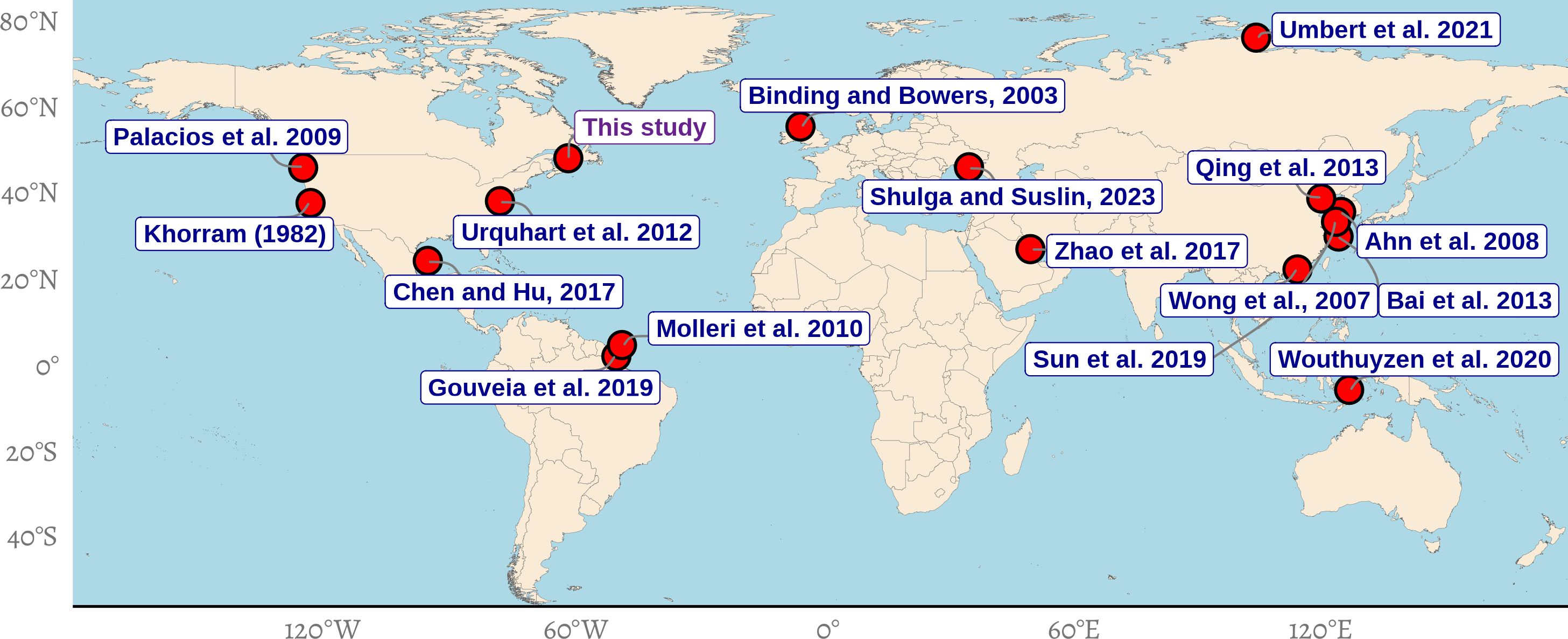
Figure 1. A non-exhaustive compilation of studies utilizing ocean color for deriving sea surface salinity (SSS). References cited: Palacios et al., (2009), Khorram (1982), Urquhart et al., (2012), Chen and Hu, (2017), Molleri et al., (2010), Gouveia et al., (2019), Binding and Bowers, (2003), Shulga and Suslin, (2023), Zhao et al., (2017), Wong et al., (2007), Sun et al., (2019), Umbert et al., (2021), Qing et al., (2013), Ahn et al., (2008), Bai et al., (2013), Wouthuyzen et al., (2020).

Unlike microwave-based techniques, no global operational methods currently address the requirements of diverse coastal systems, leading investigators to develop their own empirical models. The retrievals are commonly based on the presence of colored dissolved organic matter (CDOM), a mixture of organic material that leaches out from vegetation. Freshwater from land has low SSS values and carries large amounts of CDOM, which progressively degrades and dissolves as it is transported towards areas characterized by larger SSS (Monahan and Pybus, 1978; Massicotte et al., 2017; Laliberté et al., 2018). CDOM gives water a yellow-brown color by absorbing light more readily at the blue end of the visible spectrum, enabling SSS estimates from ocean color satellite measurements. With regards to the CDOM-SSS relationships specific to the GSLE, Nieke et al. (1997) studied the variations of absorption and fluorescence by CDOM along with salinity and found a well defined, negative linear relationship over the salinity gradient of the Upper Estuary, Lower Estuary, and Gulf. Similarly, Cizmeli (2008) measured several optically significant biogeochemical variables and found a negative linear relationship between CDOM and salinity, reporting a decrease in CDOM and an increase in salinity from west to east. Araújo and Bélanger (2022) examined the optical complexity of different water masses in the nearshore GSLE and reported strong relationships between the optical properties of CDOM and salinity. Furthermore, absorption in the GSLE was found to be dominated by CDOM in the St. Lawrence River by Xie et al. (2012), who suggested using CDOM obtained from satellites to evaluate salinity fluctuations, given that a reliable CDOM-inversion exists. All of these studies asserted the existence of a relationship between CDOM and salinity in the GSLE, yet none exploited it to predict SSS.

Here, we propose an algorithm to estimate SSS from ocean color data. We ask whether this approach, complementary to the established passive microwave approach, can offer additional insights for researchers investigating the full extent of coastal regions. Specifically, we assess the strengths and limitations of each approach based on comparisons with in situ observations and on their ability to resolve seasonal and episodic salinity dynamics across the nearshore–offshore continuum of the GSLE. The GSLE, with its extensive salinity monitoring record (Therriault, 1998), provides an ideal setting to evaluate the reliability of remote sensing products from different spectral domains in a coastal marine environment.

2 Data and methods

This section outlines our approach to synthesizing the data sources into the desired salinity products. Figure 2a showcases three data sources used in this study for a specific day, 21 June 2018. The SMAP example presents data from two overlapping scan tracks captured on the same day, with a global-scale view provided directly below. SSS has units of parts per thousand, or grams per kilogram (g kg⁻¹), representing the mass of dissolved salts relative to the mass of pure water. In situ data serves as a standard reference characterizing salinity accurately and precisely at various depths under the sea surface. Of the two satellite products used as input, one uses microwave radiometry and already describes this surface salinity (SMAP SSS L2B), and the other uses ocean color radiometry and requires conversion to salinity values (CCI Rrs). As illustrated in Figure 2b, the microwave signal is related to the salinity of the top centimeters (skin) and ocean color integrates the signal over the top meters (bulk), determined by local optical properties at the surface (Gordon and McCluney, 1975; Gordon and Clark, 1980; Bailey and Werdell, 2006). In situ measurements are limited to small spatial scales, whereas satellite methods provide synoptic views of the system but remain indirect measurements of the sea’s surface. Moreover, satellite data from different spectral domains have their own disadvantages: brightness temperature, with a large footprint, often leads to land contamination in coastal areas, while ocean color becomes useless in the presence of cloud cover. Figure 2c presents an overview of the workflow implemented in this paper, including the input, processing, output, and analyses. Each component of this flowchart is detailed in the following subsections.

Figure 2

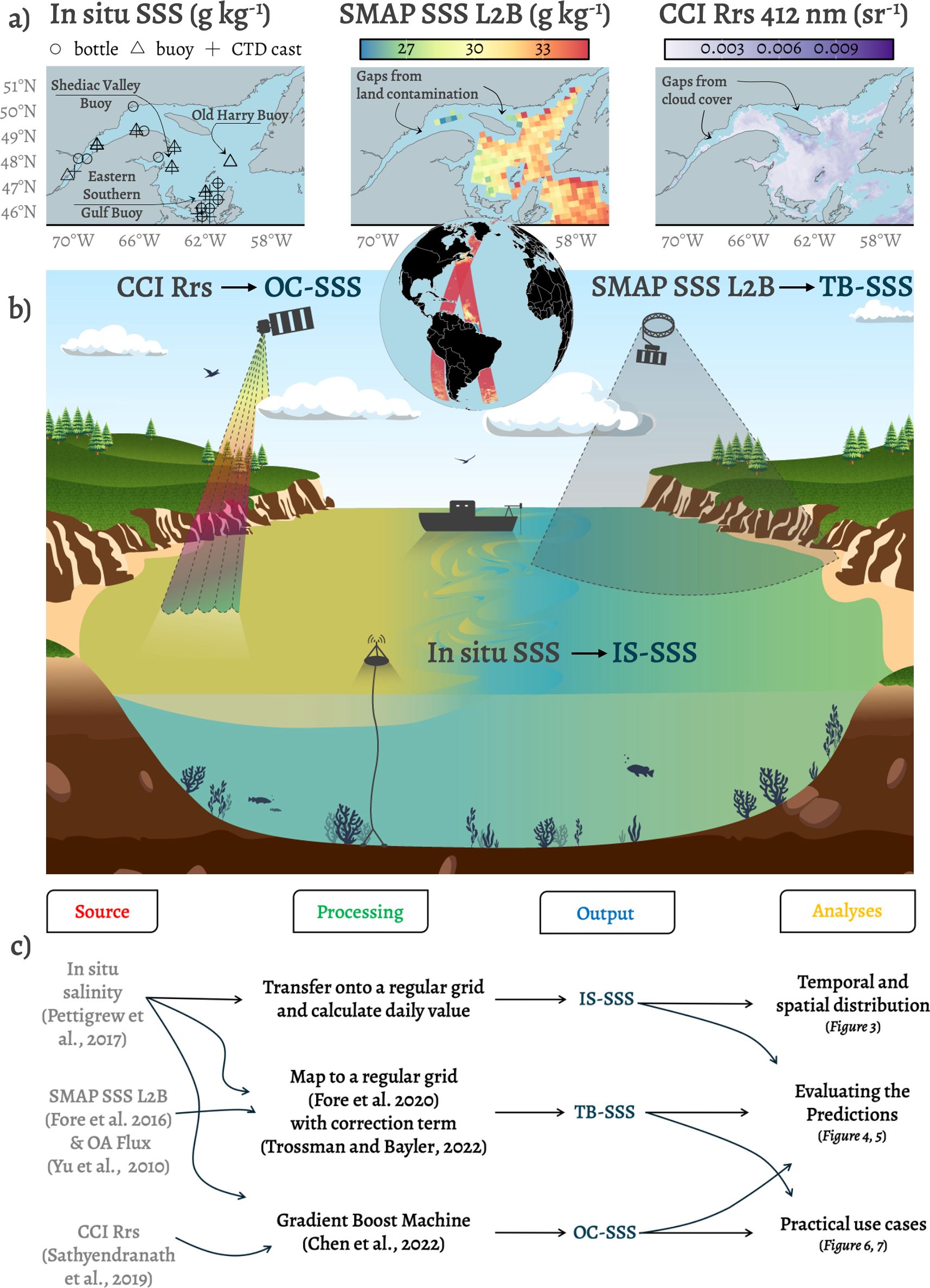
Figure 2. Summary of the methodology. (a) Examples of in situ SSS, SMAP SSS L2B and CCI Rrs at 412 nm for 2018-06–21 used as source data in this study. The SMAP SSS L2B plot displays two overlapping scan tracks captured on the same day; (b) Illustration summarizing the key differences between the products central to this research. Notably, In situ data provide sparse coverage, while ocean color data from the CCI product offer higher spatial resolution but have gaps due to cloud cover, and brightness temperature data from the SMAP product provide surface information despite clouds but are frequently affected by land contamination. (c) Flowchart illustrating the relationships between data sources, processing steps, outputs and analyses, with corresponding figures shown in italics.

2.1 Brightness temperature sea surface salinity

All SSS products derived from L-band microwaves are based on the relationship between surface emissivity and salinity. In this study, we used the SMAP-JPL data (Fore et al., 2016) as it is easily accessible online (https://podaac.jpl.nasa.gov/), which ensures broad applicability and reproducibility to other regions, and because Dumas and Gilbert (2023) determined it to have the highest correlation with in situ data in the Gulf of St. Lawrence among the microwaves products they evaluated. From the top-of-atmosphere measurements, the L-band radiometric signal undergoes land correction, galaxy correction, bias adjustments and reflector emissivity correction. Observations contaminated by land surfaces and sea ice are excluded from the dataset. Cross-track and along-track observations are rescaled to a grid with averaged fore and aft looks. Thus, four observation types are used as the main input in the JPL inversion model, representing the horizon and vertical polarizations from the fore and aft looks. This keeps track of the azimuthal dependence of the wind direction, which roughens the sea and impacts the measured brightness temperature (T_b). Wind speed and SSS are retrieved through inversion by minimizing the difference of the measured T_b and modeled T_b values, with constraints provided by ancillary wind and temperature data. We downloaded the instantaneous SMAP SSS L2B data from the PO.DAAC (NASA/JPL, 2020) for the years 2015 (beginning of SMAP operational phase) to 2023 as our source dataset (Figure 2c). Since these SSS estimates pertain only to the surface layer of the water column, we applied a conversion to minimize discrepancies with in situ measurement depths. We applied the correction of Trossman and Bayler (2022), named TB-correction, to remove bias and convert from skin-to-bulk SSS. Because of the use of in situ data, there is a smoothed version of sub-footprint variability-related adjustment likely accounted for in the correction term as well. In short, a machine learning-based generalized additive model (GAM), which is a regression framework that allows for smooth but nonlinear functions of predictors and their interactions, is used to develop a correction term. The correction term is tuned with in situ data and supplemented with the objectively analyzed air-sea fluxes product (OAFlux, Yu and Jin, 2014). The process was structured as follows:

1. In situ SSS measurements taken between the surface and 2 m depth in a given day within 25 km of the center of a grid element with a valid SMAP SSS L2B retrieval were used to compute the GAM (the SMAP-JPL product is delivered on a 25 km grid). We excluded data from 2023 from the training dataset to serve as an independent dataset for later evaluation of the satellite products. The GAM model integrates smoothers and tensor interactions of environmental predictors. The smoother terms include Julian day, the satellite-derived SSS, and a first-guess bias-correction for the satellite-derived SSS. The tensor interaction terms additionally include evaporation, latent and sensible heat fluxes, near-surface humidity, sea-surface temperature, wind stress, and auxiliary thermodynamic variables, consistent with Equation 1 and Table 1 in Trossman and Bayler (2022). The resulting predictions from the GAM, named TB-correction, were mapped onto a 0.25° longitude and latitude grid using the World Geodetic System 1984 (WGS84) and temporally averaged over the entire dataset. To map the TB-correction onto a regular grid we used a searching radius of 45 km, employing the processing methodology used in the operational L2 to L3 processing (NASA/JPL, 2020). This empirical correction reduces the disparity between the ocean color product, which captures salinity in the upper meters of the ocean, and the microwave product, which captures salinity in the top centimeters.

2. We mapped the irregular L2B satellite overpass data from 2015 to 2023 onto the same 0.25° regular grid using the same rasterization method, and subsequently applied the TB-correction across the stack of instantaneous rasters, each representing SSS from a single satellite overpass. We discarded estimates below 24 g kg⁻¹ (0.2% of the pixels) and above 36 g kg⁻¹ (3% of the pixels) to exclude large deviations from expected values, based on our knowledge of the area and corresponding in situ dataset. Since these deviations represent only a small portion of the dataset, the effects of erroneous L2B retrievals on the TB-SSS distribution are expected to be small. We removed all grid cells with fewer than five irregular L2B satellite data points mapping to a regular grid cell and filtered out all grid cells with a coefficient of variation (standard deviation divided by the mean in a 3 × 3 moving window) greater than 5%, a procedure to screen out residual retrieval failures (e.g., Werdell et al., 2009).

3. We applied a 3×3 moving window average and a 6-day rolling average to mitigate retrieval errors while preserving the dynamics of the time series. Although the operational L3 SSS product is implemented with an 8-day moving window, reflecting SMAP’s orbit repeat period, our region of interest (45.2°N–51.9°N) typically experiences two overpasses per day (Figure 2a), allowing us to use reduced smoothing. Finally, the processed data were bilinearly interpolated to match the OC-SSS spatial resolution (discussed below) before masking any data closer than 25 km from the coast. While harmonizing the spatial resolution was required for consistency, this step may introduce uncertainties and spatial smoothing, and the decision to apply a 25 km mask, although designed to ensure robustness, comes at the cost of reduced nearshore coverage, which we acknowledge as a limitation of our procedure.

Table 1

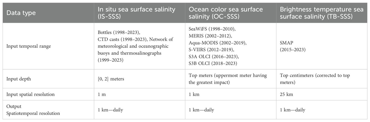
Table 1. Spatio-temporal resolutions of the products used in this study.

In summary, our processing methodology is similar to the operational L2 to L3 processing (NASA/JPL, 2020), but we included a correction term and maintained a higher temporal resolution to preserve a good representation of the dynamics of coastal oceans. We refer to this product as brightness temperature sea surface salinity (TB-SSS).

2.2 Ocean color sea surface salinity

The SSS product derived from ocean color relies on the relationship between surface color and salinity. Spectral remote-sensing reflectance (Rrs, sr⁻¹) was obtained from ocean color satellite measurements, with corrections applied for the intervening atmosphere. We downloaded merged Rrs data from multiple ocean color sensors (https://www.oceancolour.org/), processed by the European Space Agency’s Ocean Color Climate Change Initiative (OC-CCI) project version 6.0 (Sathyendranath et al., 2019). Daily composite images of visible Rrs at 1 km resolution from January 1998 to December 2023 were atmospherically corrected using the Polymer algorithm for MERIS, MODIS, VIIRS and OLCI, and the SeaDAS Standard OBPG atmospheric correction for SeaWiFS. Remote sensing values with flag warnings were removed (Jackson et al., 2022). The dataset underwent inter-sensor bias removal and spectral bands of sensors were shifted with a high-resolution spectral model to obtain six consistent bands (412nm, 443nm, 490nm, 510nm, 560nm and 665nm). Figure 2a shows an example of Rrs 412nm. For consistency, we excluded any zero Rrs values, of which only four were identified.

Next, we input the source Rrs with in situ data (excluding the year 2023) into a gradient boost machine (GBM), a machine learning method designed to estimate SSS. A GBM works by stacking simple models (i.e., ones involving small numbers of descriptors and parameters) called weak learners, that are sequentially combined into a large, more complex and more powerful model. Thus, the model partitions a challenging, hard-to-address problem into a series of simpler, easier to handle sub-problems. This approach allows each constituent model to specialize in specific aspects of the data while leaving other components to be managed by complementary tasks. Concretely, our algorithm proceeds according to the following steps:

0. Prior to any calculations, center the response on the mean value to obtain a first set of residual values using this relation:

$${\dot{y}}_i^{(0)}=y_i-\overline{y}$$

where ${\dot{y}}_i^{(0)}$ denotes the residual for observation i following the 0^th step of the procedure.

1. Fit a simple model (e.g., involving a single or a few descriptors), represented as some arbitrary function $f^{(j)}$, on the residuals as follows:

$${\dot{y}}_i^{(0)}=f^{(1)}(x_i;b)+{ϵ}_i$$

where ${\text{x}}_i$ is a vector containing descriptors associated with observation $i$, $\text{b}$ is a vector containing model parameters for these descriptors, and ${ϵ}_i$ is a model residual.

2. Apply this model at predicting the residuals of the previous step, but only partially, to obtain a new set of residuals as follows:

$${\dot{y}}_i^{(1)}={\dot{y}}_i^{(0)}- \nu f^{(1)}(x_i;b)$$

where ν is referred to as the learning rate or shrinkage and is the hyperparameter controlling how much of the model fitted values are effectively employed at shrinking the residuals, thus allowing the model to refine itself based on the data.

3. Recurse steps 1-2, adding new models, further shrinking the residuals with each step:

$${\dot{y}}_i^{(j)}={\dot{y}}_i^{(j-1)}- \nu f^{(j)}(x_i;b)$$

4. Stop after a prescribed number of steps, n, which is another hyperparameter of the model. The residuals of the model at the end of this process correspond to ${\dot{y}}_i^{(n)}={ϵ}_i$. Hyperparameters of a GBM encompass the learning rate ν, the number of sub-models n, and any parameter influencing the complexity of the sub models, such as the number of descriptors they use and any regularization parameters. The nature of sub-models, $f^{(j)}({\text{x}}_i;\text{b})$, defines the kind of gradient boosting model being implemented. For this study, we used a tree-based GBM, where individual sub-models are relatively simple (shallow) regression trees, each involving only a few descriptors. A regression tree is a model whereby the data are recursively split into sub-groups according to sets of dichotomic criteria involving the descriptors. Splitting criteria encompass threshold values for quantitative or semi-quantitative variables, or levels or groups of levels for qualitative variables. For a Gaussian response, predicted values correspond to the mean response value of the sub-groups. The tree based GBM used was XGBoost, which essentially differs from other GBM in that it implements a more stringent regularization of the sub-models, involving sub-trees that may have a lower depth than the prescribed maximum depth, $D_{max}$, set as a hyperparameter.

Next, we estimate the hyperparameters. Models have sets of quantities, called parameters, that define how they represent the data. Model estimation also involves quantities, which do not directly define the data representation, but are involved with the process by which the model parameters are estimated from the training data. By analogy, these quantities are called hyperparameters. An adequate set of hyperparameters yields a model that is generalizable across various environmental conditions. In the present study, we performed a hyperparameter search using cross-validation. Cross-validation involves partitioning the data into multiple subgroups. One or more of these groups are set aside for external validation and the remaining groups are used as the cross-validation folds. For each fold, all cross-validation data with the exception of the ones pertaining to the fold, are used to build a model and the latter is used to make predictions for the data pertaining to the fold in question. The process is repeated for all the cross-validation folds. The data of any given cross-validation fold is not used to build the model that will be used to make predictions for that fold. Therefore, the observed values and the predicted values are obtained independently from one another. The cross-validation error tends to increase whenever the model is either under- or overfitted and be minimal for an optimal model. The optimal model is the one which achieves the maximum predictive power when modeling the dataset’s response.

All available Rrs wavelengths were included in the model to make full use of the spectral information. A straightforward approach to improve predictive power involves incorporating spatial or temporal descriptors. Since the GSLE is a semi-enclosed marine system with islands and spatially heterogeneous, localized freshwater inputs, distance from the coast was not included as a predictor of salinity. Instead, we introduced temporal effects into the models by transforming the temporal information in the dataset into three derived variables. The first variable is the sampling year. This integral variable represents long-term trends over the years. The next two variables were annual sine functions representing the seasonal variations. The first sine synchronizes with the solstices, reaching +1 at the summer solstice, 0 at the autumn equinox, −1 at the winter solstice, 0 at the spring equinox, before returning to +1 at the next summer solstice, completing the cycle. Similarly, the second sine synchronizes with the equinoxes, reaching +1 at the spring equinox, 0 at the summer solstice and continues through the cycle. It is noteworthy that two variables are needed to represent seasonality. As each variable repeats its value twice a year, whereas the same pair of values occurs once a year. Because the variable year does not vary at the same scale as the two seasonal variables, and since the seasonal variables are in quadrature (90^° out-of-phase) with each other, the three variables are theoretically linearly independent. In practice, the unevenness of sampling in space and time results in non-zero correlation.

Models were estimated and then validated. For validation, the data were first sorted by increasing observed SSS values and then split into five groups systematically (e.g., data indexed by i = 1, 6, 11, 16, 21,…, were assigned to the first group, data indexed by i = 2, 7, 12, 17, 22,…, to the second group, and so on). Data sorting was used to obtain groups with similar ranges of SSS values. Data from groups 1–4 were used as the learning set to estimate the models, whereas data from group 5 were kept for model validation. For the XGBoost model, groups 1–4 served as cross-validation folds for estimating the model’s hyperparameters.

The objective criterion used for the hyperparameter estimation was the sum of square deviation between the observed y_i and predicted data ${\widehat{y}}_i,$which is defined as:

$$SSE=\sum _{i=1}^N{(y_i-{\widehat{y}}_i)}^2$$

The accuracy of the model was assessed using the square root of the SSE, which has the same units as the response (g kg⁻¹), whereas the model relative predictive power evaluated using the coefficient of prediction (P²), which is defined as:

$$P^2=1-\frac{{\sum }_{i=1}^N{(y_i-{\widehat{y}}_i)}^2}{{\sum }_{i=1}^N{(y_i-{\overline{y}}_i)}^2}$$

where $\overline{y}$ is the mean of the observed value. This metric takes the value 0 when predictions are, on average, no better than using the mean of the observed values, and a value of 1 for perfect predictions (i.e., when SSE = 0), and any negative value for models that are essentially useless (i.e., on average no better than just taking the mean observed value for all predicted values).

Hyperparameter estimation was performed using the differential evolution algorithm implemented in the DEoptim R language package (Ardia et al., 2011), with a population size of 30 individuals over 200 generations. The raw hyperparameters controlling for the number of trees and maximum tree depth were raised to the power of two and rounded to the closest integer before being used by the model estimation function, whereas the raw hyperparameter controlling for the learning rate was inverse logit-transformed prior to its use. These transformations of the parameter space were meant to help in the searching process by covering a broad array of values of the number of trees and maximum tree depth with slight fluctuations of the parameter value while ensuring that the learning rate was strictly bounded between 0 and 1.

We estimated the among-year model accuracy and predictive power by training models with data from previous years to predict data from a given year. We performed that exercise in a backward manner beginning from the year 2022 down to the year 1998. As with the TB-SSS product, the year 2023 was omitted in the training dataset to serve as an independent basis for later evaluation of the satellite products. Once the model was completed, we produced the SSS predictions. We refer to the output as ocean color sea surface salinity (OC-SSS).

2.3 In situ measurements

The Department of Fisheries and Oceans Canada collects and hosts a large number of in situ surface salinity measurements. Samples from 6,856 bottles, 31,524 CTD casts and 1,924,556 measurements from meteorological and oceanographic buoys and deployed thermosalinographs were available in the Oceanographic Data Management System (Pettigrew et al., 2017) between 1999 and 2023 across the GSLE. Salinity data collected through flow-through systems on multiple vessels were also available, but were not used due to the difficulty in determining the measurement depths, which varied based on ship bow shapes and speeds. Bottles captured water at specific depths and were subsequently analyzed using either Guildline Portasal (ship-based) or a Guildline Autosal (lab-based). Both data types were compiled by the lab technician who produced triplicate measurements of 10 readings per bottle after flushing with millipore water, allowing for robust quality control in resulting salinity data. The CTD instruments were calibrated every winter by electronic technicians. On ships, CTD profile measurements recorded conductivity after a three-minute surface soak allowing the instrument to adjust to local water conditions. Discrete samples were routinely compared to CTD casts since both record salinity subsequently. On buoys, the CTD instrument usually took a measurement every 15 minutes during the open water season. Of particular interest to this study are the Banc des Orphelins, Shediac Valley, Old Harry and East Southern Gulf buoys located in Gulf of St. Lawrence, which provide highly resolved time series at fixed locations. Trained data analysts oversaw the incorporation of new data and assigned a flag to each entry, which ensured realistic values. The largest uncertainty sources for salinity stem from the depth uncertainties. Accordingly, we decided to keep all data from the 0 m to 2 m to represent surface waters. We gridded in situ salinity measurements by aggregating measurements falling within a grid element over a UTC day time and over the depths. Since buoys are assessed independently in one of our evaluations, we kept different types of measurements (buoys, profiles, or bottles) separated when more than one type was available. We refer to this dataset as in situ sea surface salinity (IS-SSS).

2.4 Matching observations

A common spatial and temporal resolution for this study was defined by the finest resolutions available from satellite data, that is, a nominal spatial resolution of 1 km with a daily time scale. Table 1 summarizes the characteristics of the three main sources of data used in this study.

After gridding the in situ data and producing the satellite output, we designed a set of analyses to explore the satellite products (see Figure 2c, Analyses). We first examined the characteristics of the temporal and spatial distribution of data. To this end, we computed the number of predictions for each method, as well as the SSS mean value (µ), for each grid element ($i$, $j$) over time ($t$).

$${\mu }_{i,j}=\frac{1}{n}\sum _{t=1}^n{X}_{i,j,t}$$

Second, matchups between in situ SSS and the two satellite products were used to evaluate the predicted values. We adopted the root mean square difference (RMSD) as a metric for evaluating the performance of the satellite products, as well as P² (coefficient of prediction) defined above, accompanied by the number of observations. We also leveraged the fact that many pixels had multiple observations within a single day, taken at different times or from different locations within the 1 km pixel. This range was used to assess whether the estimate fell within the observed variability during the matchup exercise. Additionally, in the context of evaluating the predictions, we gain further insights by analyzing buoy time series alongside satellite-derived time series, enabling us to observe the dynamics of SSS products. As previously mentioned, the year 2023 was excluded from the training of satellite models to provide an independent basis for evaluation; consequently we used the buoy time series from that year for this analysis. Finally, we present practical use cases to illustrate how the two satellite products function in practical research applications. We assess whether these products lead to similar conclusions when analyzed from different perspectives. Specifically, we examine freshwater pulses through time series and explore the impact of a post-tropical storm on salinity maps. Through these tangible applications, we aim to highlight the strengths and limitations of TB-SSS and OC-SSS.

3 Results and discussion

3.1 Temporal and spatial distribution

One of the key findings of the present study is the difference in the number of salinity estimates available in the different products. Figure 3 presents the mean number of monthly estimates from IS-SSS, OC-SSS and TB-SSS datasets, with their spatial coverage illustrated by the SSS mean.

Figure 3

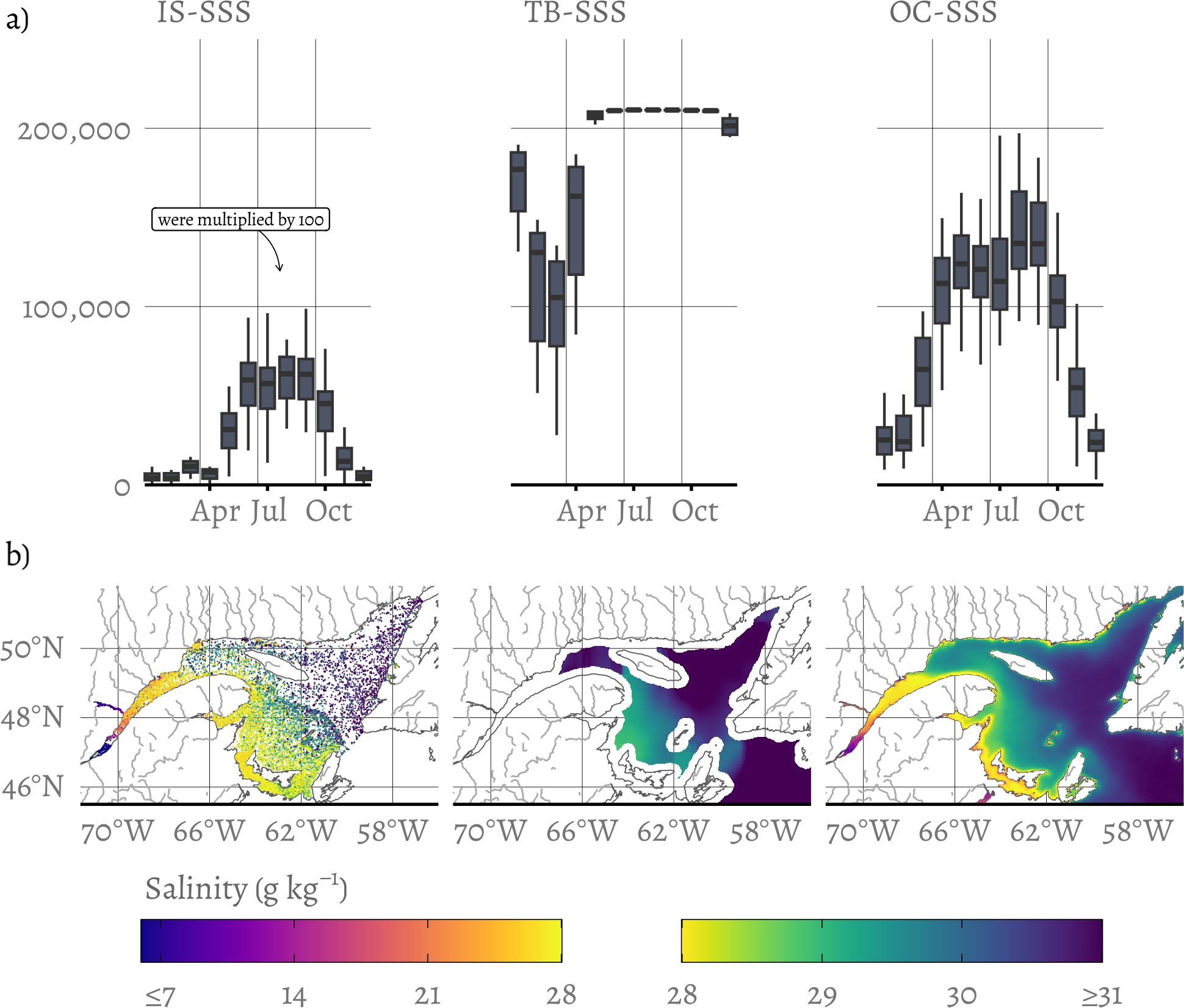
Figure 3. Temporal and spatial distribution of available surface salinity values from in situ (IS-SSS), ocean color (OC-SSS) and brightness temperature (TB-SSS); (a) The top panel shows the distribution of monthly data counts from January to December summarised over all years using boxplots, calculated based on the 1 km grid and daily time resolution shared by all three datasets. The IS-SSS values were multiplied by 100 to align them with the scale of the other plots; (b) The bottom panel displays the extent of data availability color-coded by salinity values, represented by the SSS mean for satellite observations. The color scale transitions at two different rates within the color space, one for each palette.

Based on the climatological cloud fraction, sun zenithal angle and sea ice cover (Appendix A), Figure 3a can be described in three segments. From April to October, IS-SSS has the least available data as expected, despite most field campaigns being conducted during this period, followed by OC-SSS. TB-SSS provides the most data, primarily because it captures information of the surface even under cloudy conditions. From November to January, when the sea surface is predominantly ice-free (Galbraith et al., 2024b), this difference between the satellite products is even more pronounced. At this time of year, the sun remains low and cloudy conditions prevail, resulting in fewer valid Rrs and thus fewer OC-SSS estimates (Clay and Devred, 2023; Laliberté and Larouche, 2023). During the February-March period, both satellite methods are unable to capture information below sea ice. In fact, the reduced availability of data is evident across all products (Figure 3a). In situ data are underrepresented because buoys are not deployed during winter to avoid the crushing damage caused by sea ice. As for the satellite products, certain regions with partial ice-cover are best observed with ocean color satellites, whose finer spatial resolution enables observations between sea ice floes, providing data in inaccessible and rarely studied environments. Conversely, microwave satellite sensors, with their coarser resolution, can suffer from subpixel contamination caused by sea ice, resulting in inaccurate and unreliable SSS retrievals (Fournier et al., 2019; Meissner and Manaster, 2021).

Across the GSLE, IS-SSS accounted for only 0.3% of OC-SSS data, which itself represented 55% of TB-SSS data (Figure 3a). Although there are many OC-SSS estimates in the estuary and nearshore, TB-SSS has a considerably greater amount of estimates offshore. In fact, in offshore areas where TB-SSS estimates were available, coincident OC-SSS data were found in only 29% of cases.

Figure 3b shows that the western GSLE has lower salinity (below 28 g kg⁻¹) than the eastern GSLE (above 28 g kg⁻¹). The highest in situ value of the dataset is 33 g kg⁻¹. Figure 3b allows for a qualitative comparison between products. The Estuarine and Southern Gulf regions have the most extensive in situ coverage, but the salinity gradient from west to east, as suggested in the figure, lacks sharp definition. Each panel displays the low-salinity water outflow from the St. Lawrence Estuary, forming the Gaspé Current, which spreads towards the Magdalen Shallows and over Cape Breton. Other secondary features, such as the freshwater input from the North Shore rivers, are visible in the OC-SSS product. These freshwater inputs quickly mix with offshore saltier water and generally do not extend far into the Gulf. Accordingly, these features are not visible with TB-SSS due to land contamination caused by the coarse native spatial resolution.

In summary, the limitation of the OC-SSS is obvious from the number of monthly estimates (Figure 3a), while the limitation of TB-SSS is obvious from the spatial coverage and resolution (Figure 3b).

3.2 Evaluating the predictions

The instantaneous and punctual in situ data were merged into 87,138 observations mapped to the daily 1 km grid for comparison with the satellite data. Of these, only 36,799 observations were collected after 2014, when both satellite products were available. Figure 4 shows the observations matching valid satellite retrievals over this period, along with their corresponding evaluation metrics. More details on the OC-SSS predictive model are provided in Appendices B, C.

Figure 4

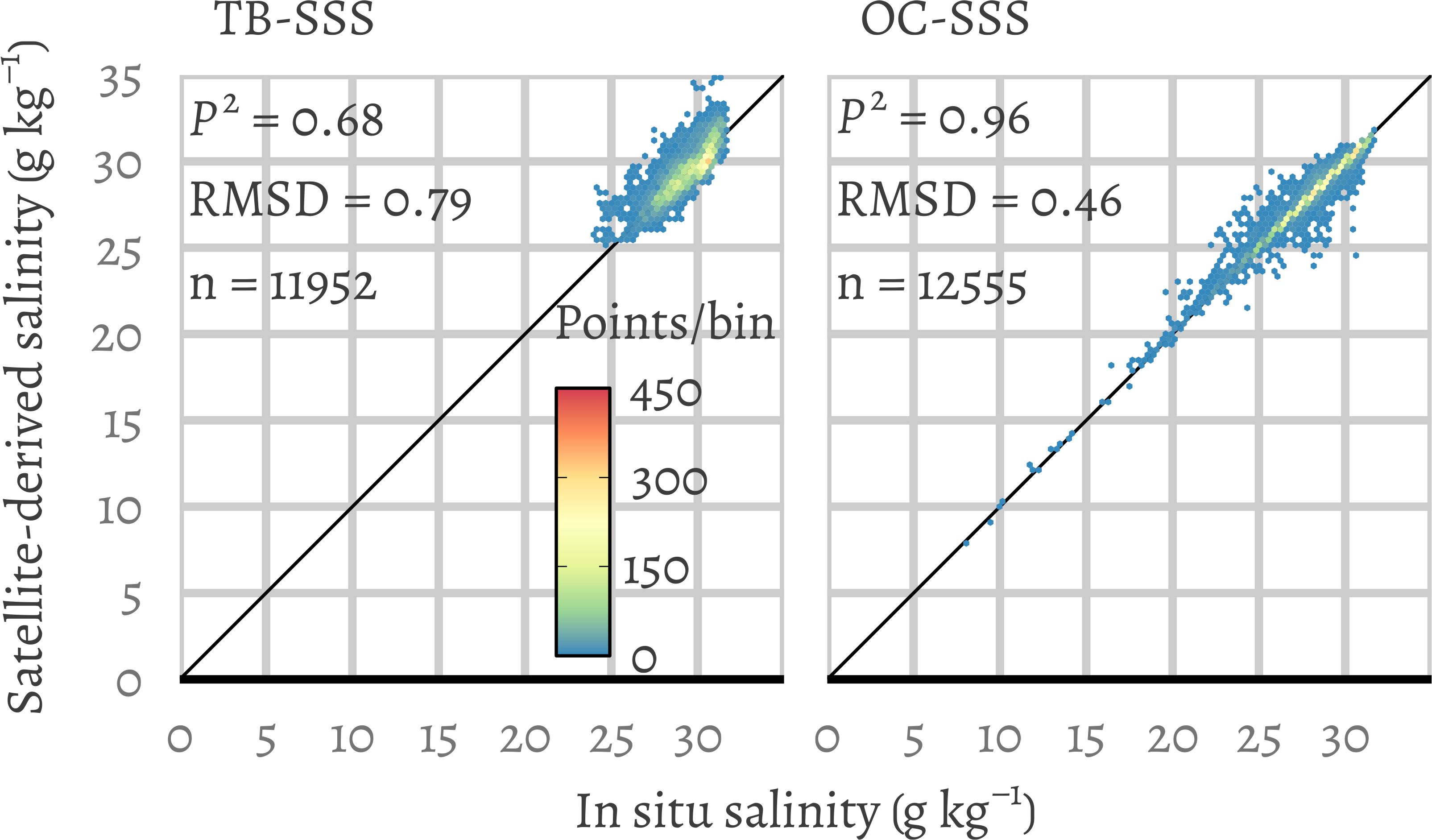
Figure 4. Scatterplot comparing satellite-derived products with in situ data. The left panel shows TB-SSS against in situ measurements, while the right panel presents OC-SSS compared to in situ data. The coefficient of prediction (P², dimensionless), root mean square difference (RMSD, g kg⁻¹) and number of observations (n, unitless) are shown in the scatterplots.

Contrary to expectations, there are more matchups with the ocean color product, because nearshore salinity measurements are easier to collect than offshore ones (Figures 2a, 3b). TB-SSS are clustered in salinity levels exceeding 25 g kg⁻¹, primarily due to the lack of estimates in nearshore areas where the salinity is typically lower. The TB-correction improved the RMSD by 0.22 g kg⁻¹, further enhancing agreement with in situ observations. Moreover, the combined effect of the correction, gridding, filtering, and smoothing steps reduced the RMSD by about 1.3 g kg⁻¹, relative to direct matchups with raw L2B data. The points from OC-SSS align well with IS-SSS, even at low salinity values. Compared with TB-SSS, the OC-SSS matchups cluster more tightly around the one-to-one line, with evaluation metrics indicating superior performance. Furthermore, by utilizing the intra-day and intra-pixel variability from in situ measurements, we found that 47% of OC-SSS estimates were within the daily range of salinity for a pixel, while only 10% of estimates for TB-SSS were within that range. Nevertheless, the difference between measurements and satellite estimates may only serve as an imperfect metric of their precision and accuracy, because most matchups were also used to train the GBM and served to define the TB-correction, and consequently, the objectivity of this assessment is limited. To offer a complementary perspective, we exploit buoy measurements from the year 2023, which were not used to develop the products (Figure 5).

Figure 5

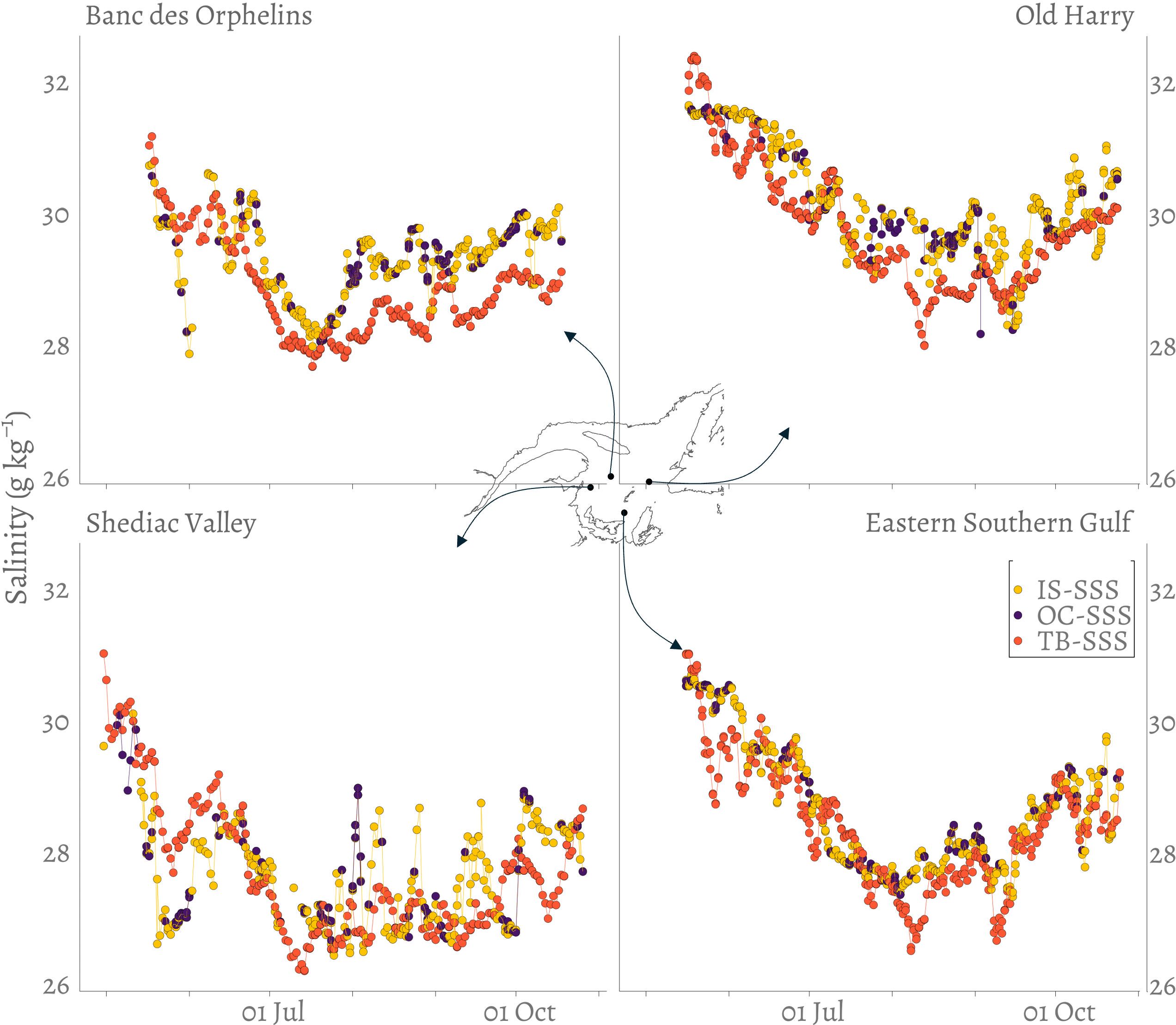
Figure 5. Dynamics of the satellite products at a daily time scale shown for the year 2023. The seasonal variability of IS-SSS at the Banc des Orphelins, Old Harry, Shediac Valley and Eastern Southern Gulf buoys compared to the OC-SSS and TB-SSS products extracted at those locations. Note that the year 2023 was excluded from the training of satellite products.

All TB-SSS estimates coincided with an IS-SSS data point, whereas only 30% of OC-SSS estimates matched data in the buoy time series, a ratio that is comparable to the one reported above (29%). The longest gaps in the OC-SSS time series lasted 14 days at Old Harry in July, 13 days at Shediac Valley in September, 12 days in the Eastern Southern Gulf in September, and 11 days at Banc des Orphelins in June. Here again, OC-SSS aligned more closely with the measurements. The RMSD for OC-SSS (0.06 g kg⁻¹) is considerably lower than that of TB-SSS (0.68 g kg⁻¹), and lower than those shown in Figure 4. The strong retrieval performance of OC-SSS is largely due to the abundance of training data from similar environmental conditions, often obtained from the same buoys prior to 2023. Because the training and validation datasets include these highly resolved time series, spatial clustering likely inflate performance metrics, which represents a limitation of our analysis. For the other matchups of 2023 (other buoys, bottles, and profiles), the performances were comparable for TB-SSS (0.79 g kg⁻¹) and slightly worse, though still better than for the entire dataset, for OC-SSS (0.30 g kg⁻¹). Although the buoys are located at varying distances from land (roughly 40 km for Shediac Valley and Eastern Southern Gulf, and about 70 km for Old Harry and 100 km for Banc des Orphelins), the RMSD values are similar across sites (0.778, 0.539, 0.644, and 0.776 g kg⁻¹, respectively), confirming that land contamination is not the main driver of discrepancies. Overall, the retrieval performance of TB-SSS compares favorably with the evaluation of the SMAP-JPL L3 product over the global coastal ocean reported by Jarugula et al. (2025), where the average RMSD exceeded 1.49 g kg⁻¹.

Different mechanisms affect the salinity at the different buoy locations. An important result from Figure 5 is that the overall seasonal cycle is well captured by both satellite products, despite the different mechanisms influencing salinity at the various buoy locations. However, transient or localized events are better detected by OC-SSS, while TB-SSS exhibits greater variability around the rapidly fluctuating IS-SSS time series. This variability sometimes appears as an overestimation and other times as an underestimation relative to in situ measurements. Part of the discrepancy with in situ measurements in the TB-SSS time series can be explained by unresolved submesoscale processes in the water volumes observed by the sensors, which ultimately leads to lower performance metrics (Boutin et al., 2016).

3.3 Practical use cases

3.3.1 Freshwater transfer variability

We analyzed the satellite data record to investigate salinity variability associated with the movement of water between the land and the Atlantic Ocean (Figure 6). We included flows through major surface circulation features of the Gulf of St. Lawrence (GSL), specifically the transfer from the Gaspé Current (-63.7°, 48.8°), the northeast GSL, likely influenced by inflow from the Strait of Belle Isle (-60.0°, 49.9°), as well as inflow through the Cabot Strait (-59.90°, 48.0°). To study this variability, we extracted all pixels within a 12.5 km radius (25 km diameter circle) for these three key locations. A 14-day running mean was applied to smooth each product’s three extracted time series. The distribution of the series, represented by the 10th to 90th percentiles of all values, was calculated for each satellite product. We highlighted the years 2017 and overlaid it on the percentiles, as Galbraith et al. (2024a) indicated that the year 2017 had among the largest annual freshwater runoff since 1974.

Figure 6

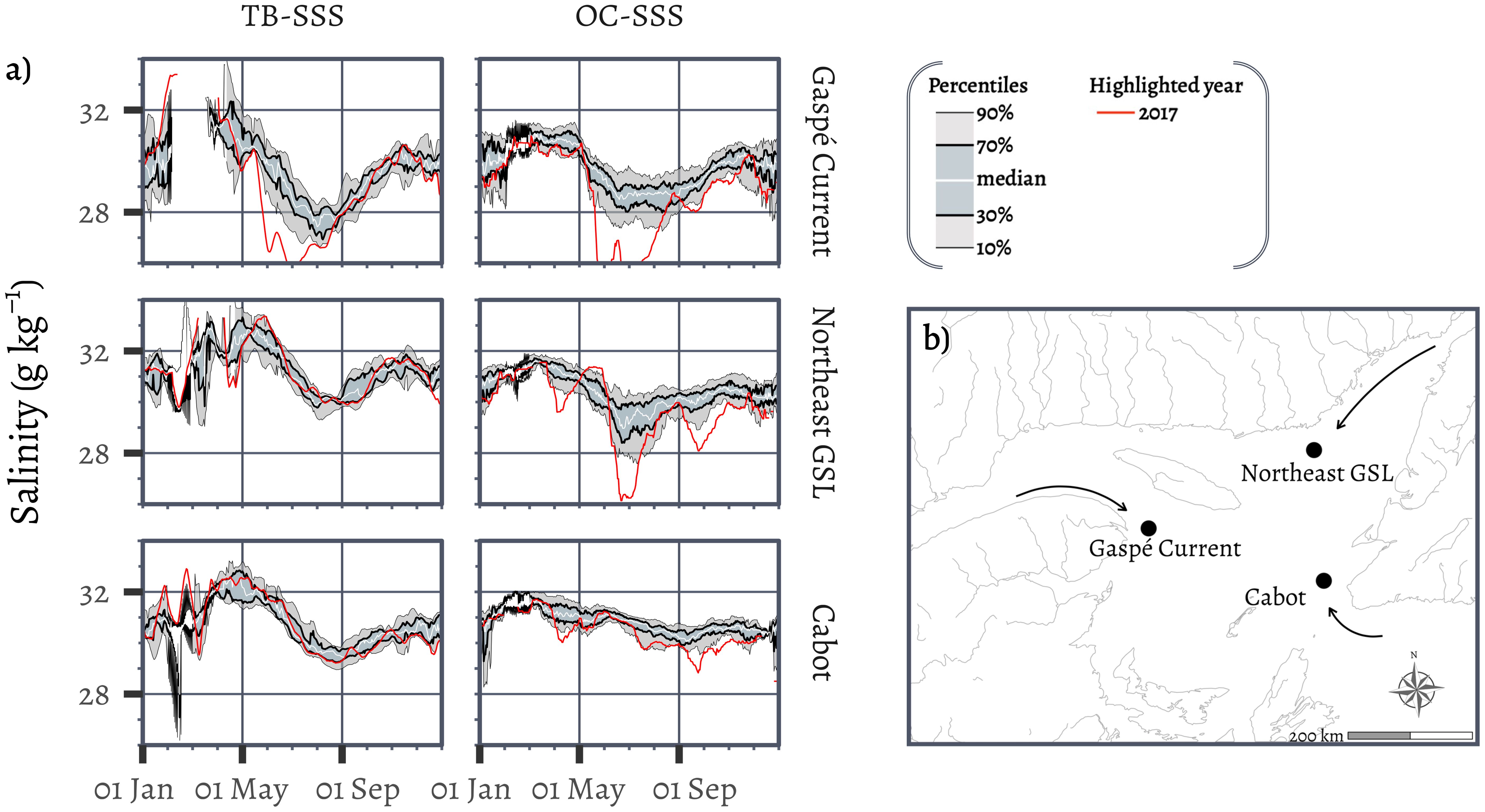
Figure 6. Salinity variability in three major circulation features of the Gulf of St. Lawrence; (a) The percentile distribution of salinity for the OC-SSS and TB-SSS satellite products in the Gaspé Current, northeast GSL, and Cabot Strait regions along with observations for 2017; (b) Map showing the 25 km diameter polygons used to extract the time series data from the satellite record, along with the main surface currents flowing toward these areas.

First, we examine the results from the percentile distribution (Figure 6a, ribbons), as comparing these distributions reveals general patterns of seasonal variations. Early in the year, large variations and breaks in the time series occur because of sea ice, with the longest period of missing data occurring in the Gaspé Current. Sea ice is typically present for longer periods in the Gaspé Current region due to its role in transporting sea ice from the St Lawrence Estuary (Galbraith et al., 2024b). A small fraction (less than 0.4%) of the values from the OC-SSS time series during February and March were found to be suspiciously low. Investigation with sentinel-2 higher resolution true color satellite images showed that a mix of sea ice made it through the CCI flagging and thus unrealistic values were produced by the GBM. Bélanger et al. (2007) previously documented this issue, demonstrating that specific configurations of ice floes can influence Rrs due to adjacency effects and sub-pixel contamination. These salinity retrievals had to be manually removed, warranting that caution should be used when using ocean color data in subpolar regions. During winter, following brine rejection, the values peak for the year across all extracted time series and both products. However, pinpointing the exact timing of this maximum is challenging due to missing data early in the year. Salinity decreases due to snow and sea ice melt along with spring runoff, reaching a minimum in summer. This pattern is consistent with expectations (Galbraith et al., 2024a), indicating that runoff outweighs the combined effects of evaporation and precipitation. The cycle is seen in both products. For the Gaspé Current location, the minimum in the OC-SSS time series remains stable for a period starting in mid-June for OC-SSS and in mid-July for TB-SSS, continuing to September for both products. At the northeast GSL location, the minimum spans from mid-June to early August for OC-SSS, and from August to October for TB-SSS. For the Cabot Strait location, both products show a minimum in September, with the timing of the minimum slightly shorter and later here than at other locations. After reaching this minimum, salinity gradually increases, likely due to a combination of factors including changing heat fluxes, fall precipitations and wind stress, eventually leveling off at fall levels, which lie between the spring and summer salinity values. Overall, both products discern more pronounced seasonal variations in the Gaspé Current and northeast GSL compared to Cabot Strait. However, the timing of these events does not always align precisely between the two products. Notably, seasonal variations are also more prominent in TB-SSS than in OC-SSS.

We now discuss the year 2017, which stands out in the data record for its distinct salinity patterns, as presented through the two satellite products (Figure 6a, red lines). In the Gaspé Current area, two freshwater pulses were observed in each product. The first pulse occurred in late May for OC-SSS and early June for TB-SSS. The second, longer pulse was detected at the end of June in both products. Here, the two satellite-derived SSS show agreement in the timing of events, with both pulses exhibiting minima within three days of each other when compared across the two products. The peak of freshwater runoff at Québec City, much further upstream, shows a maximum in April and May in 2017 (Fisheries and Oceans Canada, 2023). Despite noting stronger seasonal variations in the distribution of percentiles for TB-SSS above, here the OC-SSS product shows slightly more extreme values, with minimum salinities of 23 g kg⁻¹ compared to 26 g kg⁻¹, and 25 g kg⁻¹ compared to 25.8 g kg⁻¹ (outside the plot, to preserve scale). In contrast, the 2017 minimum of northeast GSL Strait is evident in OC-SSS, where a low salinity plume appeared to stretch unusually far from the North Shore towards Newfoundland over the extracted zone (not shown). However, this 2017 minimum does not appear in the corresponding TB-SSS time series. There were no in situ data in that area to verify the magnitude of this plume. In comparison with the two other locations, both 2017 time series at the Cabot Strait location show little difference relative to the percentile distribution, as would be expected given the current direction shown in Figure 6b. Together with the metrics from the evaluation section, these findings suggest that short-lived events tend to more accurately captured by the OC-SSS product while they are smoothed out in the TB-SSS product. Apart from studying differences between salinity products, this type of analysis could be used to track harmful algal blooms, since such events are known to occur under unusually low salinity conditions (Boivin-Rioux et al., 2021; IOCCG, 2021). Deviations from typical seasonal cycles could be identified and further examined through ocean color radiometry that enables retrieval of phytoplankton functional types, either retrospectively or continuously using near-real time satellite information.

3.3.2 Impact of a post-tropical storm

Hurricane activity has increased in the Western Atlantic over the past 50 years (Lopez et al., 2024). For example, on 7 September 2019, Hurricane Dorian approached the southern coast of Nova Scotia and continued through the GSL as a post-tropical storm on September 8. Severe winds, and important precipitations ensued; 13 m waves, winds of 120 km h⁻¹ and a remarkable drop in surface water temperature of 8 °C was recorded at the Eastern Southern Gulf buoy (location shown in Figures 2, 5, Galbraith et al., 2020; Galbraith, 2022). The severe winds induced mixing, bringing saltier water up to the surface, while precipitation added fresh water. Figure 7 presents the resulting effect of that hurricane on the surface salinity of the GSL.

Figure 7

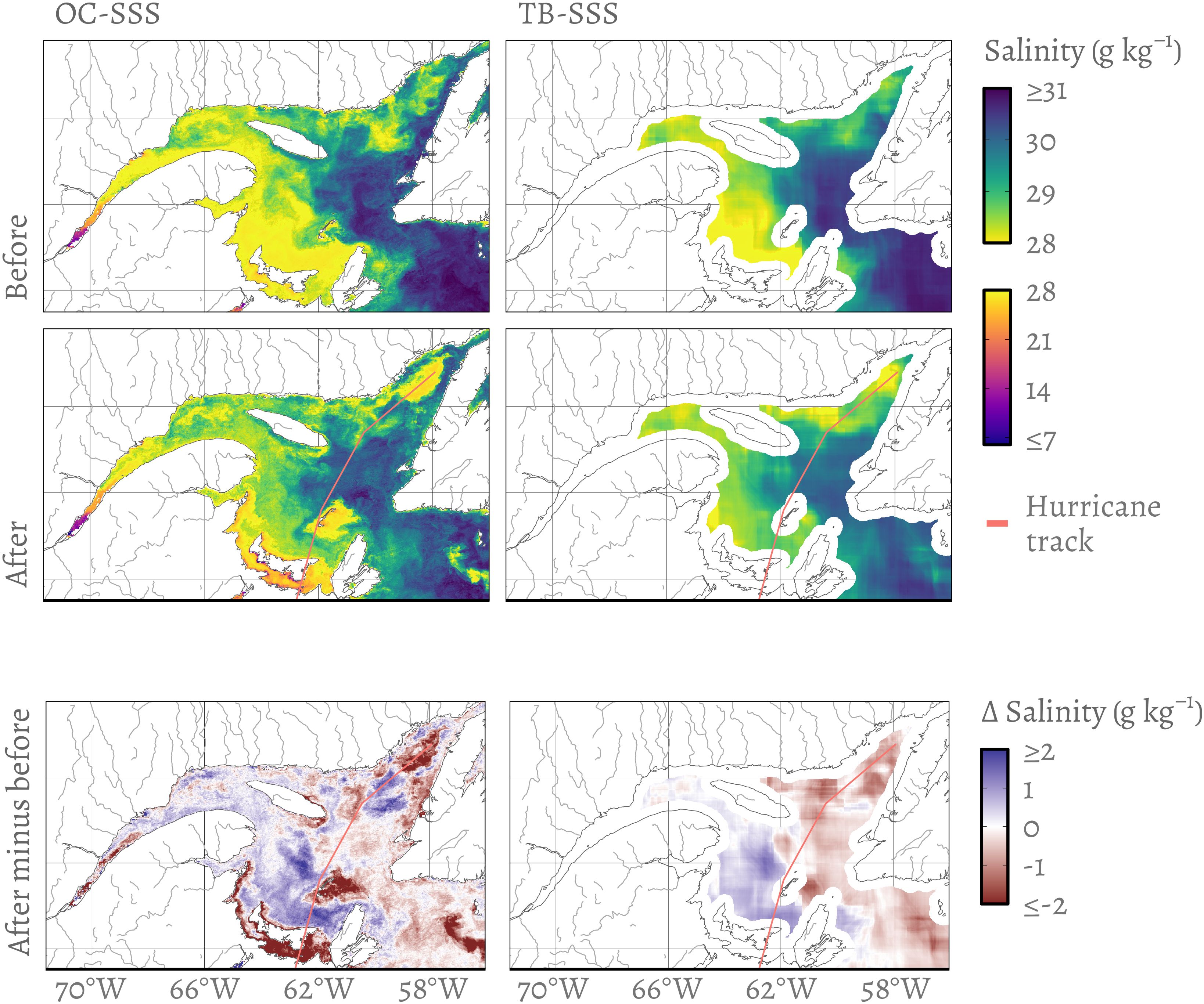
Figure 7. Satellite-derived salinity during Dorian’s passage over the Gulf of St. Lawrence. The upper panels display salinity maps obtained by averaging the OC-SSS and TB-SSS products over the week before and the week after the event, with the hurricane track overlaid in red (Landsea and Franklin, 2013). The lower panels show the difference in salinity between these two periods.

Both products successfully reveal that the storm created a saline wake (an increase in surface salinity) in the western GSL and a fresh wake (a decrease in surface salinity) in the eastern GSL. While differences in magnitude are observed, the spatial patterns are consistent across the products. The TB-SSS product, as expected, shows a more subdued temporal contrast.

The largest increase are seen over the Magdalen Plateau, where shallow waters were mixed, leading to higher salinity levels. The aforementioned buoy recorded mixing down to 45 m depth and an increase of surface salinity of 3 g kg⁻¹ and equal average salinity between 0 and 45 m before and after the storm, suggesting that vertical mixing was responsible for the change. When considering only the OC-SSS product, it could be inferred that the strong decrease in salinity in the southeast of Magdalen Plateau is linked to increased turbidity in these shallow waters, potentially confounding the GMB algorithm. However, in the TB-SSS product, which operates in a different spectral domain and uses a different underlying principle to retrieve salinity, reduced salinity values are also observed.

Figure 7 clearly demonstrates that post-tropical storm Dorian had a direct impact on the density structure of the upper water column throughout the GSL. We can speculate that mixing drew phytoplankton to greater depths while replenishing the illuminated portion of the water column with nutrients, thereby impacting primary production (Davis and Yan, 2004; Fuentes-Yaco et al., 2005; Son et al., 2006). Figure 7 also illustrates the indirect impact of lagged freshwater runoff following inland flooding and land drainage, as evidenced by the OC-SSS product showing low-salinity water masses in the St. Lawrence Estuary and Northumberland Sound, which will gradually dissipate while flowing towards Cape Breton. Beyond comparison purposes, this type of analysis could help assess the impacts of tropical cyclones on coastal marine ecosystems. Combined with sudden decreases in sea surface temperature detected from satellite remote sensing, increases in surface salinity over the same area could be used to infer mixing depth associated with the passing of a storm.

4 Conclusion and perspectives

Reliable estimates from satellite observations can help assess how well ocean models represent a region and its mesoscale processes (Meadows, 2009; Le Fouest et al., 2006), or strengthen existing ocean observation networks by complementing in situ measurements with additional data on the oceanic state (Dumas and Gilbert, 2023; Vinogradova et al., 2019). Considering this, we have evaluated two sea surface salinity (SSS) products retrieved from two distinct spectral domains over the St. Lawrence Estuary and Gulf (GSLE). We have chosen the SMAP-JPL product to represent the microwave-derived salinity (TB-SSS), which estimates salinity from the algorithm of Fore et al. (2016). Future research could also explore deriving TB-SSS directly from satellite-measured brightness temperature values and in situ data, or incorporating blended microwave datasets such as CCI-SSS (Boutin et al., 2021). A cross-comparison against other satellite SSS products could provide additional perspective on large-scale bias and regional consistency. Our study illustrates that nearshore and small hydrological features are impossible to detect with the current generation of salinity satellites and supports the need for higher spatial resolution satellite sensors (Rodríguez-Fernández et al., 2024). However, TB-SSS provides an informative view of the more offshore large-scale circulation with notable temporal accuracy, as microwaves provide information on the surface even in cloudy conditions. Conversely, when harnessing ocean color to obtain sea surface salinity (OC-SSS), key nearshore features can be resolved, for instance, the density front separating fresher and saltier surface waters at the boundary of the Gaspé Current (Cyr and Larouche, 2015; Leclercq et al., 2024). In addition, the two practical use cases we presented showed that short-lived events are best represented with this product, and the evaluation metrics indicated that OC-SSS demonstrates superior performance over TB-SSS in the GSLE. It follows that the OC-SSS product emerges as particularly promising for coastal studies. Nevertheless, some salinity values from OC-SSS were found to be suspicious in the presence of sea ice, showing incomplete flagging. We also suspect that a sudden increase in turbidity could lead the algorithm astray. Although retrieved OC-SSS values after tropical storm Dorian in 2019 were corroborated by the TB-SSS product, which operates on drastically different principles, it is not a demonstration of immunity against such stray values. Importantly, the OC-SSS product accurately reflects the conditions for which it was trained, but Rrs–SSS relationships are subject to change with space (e.g., Appendix D) and time (e.g., under climate change). Across the overlapping spatial region, our findings support the idea that these two products should be combined, whenever possible, to mitigate their limitations.

There is a clear need for satellite products that provide investigators with high-resolution, high-quality data extending continuously to the shoreline, enabling detailed analysis of coastal dynamics, notably without gaps in space and time. Now that we have demonstrated how two contrasting spectral domains each offer different strengths and limitations yet can retrieve the same key variable, SSS, a new question arise: could multivariate reconstructions (i.e., gap-filling) of the OC-SSS field outperform univariate approaches? A univariate reconstruction rests on the idea that nearby locations and adjacent days are similar to the current time and place, which depends heavily on the relation between the resolution of the product and the heterogeneity of the studied variable. Alvera-Azcárate et al. (2007) approached this problem and argued that complementary variables with some degree of correlation with the variable of interest should be used to help fill the gaps. They utilized wind data from the SeaWinds scatterometer and chlorophyll-a data from Aqua to reconstruct sea surface temperature (SST) from AVHRR. In our case, we could argue that the flux of incident shortwaves impacts ocean’s stratification and that such operational products could be leveraged to improve the reconstruction of SSS fields. Satellite estimates of incident shortwaves are obtained in the presence of clouds and thus increase the amount of information available on the surface in the absence of OC-SSS estimates. SST could also help in reconstructing SSS as it can be derived during nighttime, and because it can be acquired from satellites having different equatorial crossing times, which again increases the likelihood of having valid information on the environment close to the desired time/space. The key challenge here lies in capturing the hard-to-quantify, dynamically changing relationship between those ancillary variables and SSS (indirect predictors). Covariance with ancillary variables may be adequate at basin or seasonal scales, but might not work as effectively at finer resolution and in coastal areas where complex submesoscale processes make SSS highly heterogeneous. We believe that in future efforts, gap-free salinity estimates from ocean color remote sensing should be guided by the same variable (direct predictor) estimated from independently derived salinity fields obtained through microwave remote sensing with different inherent constraints, having in principle a correlation level that should be approaching unity. Despite having a coarser spatial resolution (requiring a degree of downscaling), the contribution of the microwave spectral domain ensures the missing data never persists in time, preserving a lower degree of uncertainties over that dimension. The applicability of that direct predictor would be limited to coastal areas with large estuary influence such as those presented in Figure 1; yet, these marine systems are arguably among the most ecologically and economically important worldwide. This innovative approach would likely outperform single products, or conventional interpolation techniques reliant on a single spectral domain, thereby enhancing the quantity and reliability of the resulting salinity assessment.

Data availability statement

SMAP SSS L2B data are available at https://podaac.jpl.nasa.gov/. CCI Rrs data are available at https://www.oceancolour.org/. The XGBoost model for ocean color is available from the corresponding author upon request. Monthly OC-SSS are available on the SLGO website (https://doi.org/10.26071/ogsl-969715ba-3747).

Author contributions

JL: Conceptualization, Data curation, Formal analysis, Investigation, Methodology, Software, Validation, Visualization, Writing – original draft, Writing – review & editing. GG: Formal analysis, Software, Writing – original draft, Writing – review & editing. JD: Writing – original draft, Writing – review & editing. PG: Writing – original draft, Writing – review & editing. SH: Writing – original draft, Writing – review & editing. DT: Software, Writing – original draft, Writing – review & editing. SV: Writing – original draft, Writing – review & editing.

Funding

The author(s) declare financial support was received for the research and/or publication of this article. DT was supported by NOAA grant NA24NESX432C0001 (Cooperative Institute for Satellite Earth System Studies - CISESS) at the University of Maryland/ESSIC. SH received funding from Global Science and Technology, Inc. The funders were not involved in the study design, collection, analysis, interpretation of data, the writing of this article or the decision to submit it for publication.

Acknowledgments

We sincerely thank all the staff who contributed to making salinity data accessible, and in particular, Marie-Noëlle Bourassa. Special appreciation goes to those responsible for in situ data collection, including participants in oceanographic missions, as well as those involved in equipment maintenance, calibration, and data management. We are grateful to the teams who developed and delivered the ocean color and brightness temperature products for the satellite data, including staff at JPL, NASA, and ESA. We thank Dr. Alexander Fore for useful discussions and Solène Paumier for her assistance with the graphical design. Calculations were carried out using the R language and environment (R Core Team, 2021). General data processing was performed using R packages magrittr (Bache and Wickham, 2022) and RSQLite (Müller et al., 2024), and geographic data processing using R packages sf (Pebesma, 2018) and raster (Hijmans, 2018). XGBoost models were calculated using Rpackage xgboost (Chen et al., 2020) and hyperparameter estimation was carried out using standard R package stats.

Conflict of interest

Author SH was employed by Global Science and Technology.

The remaining authors declare that the research was conducted in the absence of any commercial or financial relationships that could be construed as a potential conflict of interest.

Generative AI statement

The author(s) declare that Generative AI was used in the creation of this manuscript. Generative AI was used to verify the grammatical correctness of the English text.

Any alternative text (alt text) provided alongside figures in this article has been generated by Frontiers with the support of artificial intelligence and reasonable efforts have been made to ensure accuracy, including review by the authors wherever possible. If you identify any issues, please contact us.

Publisher’s note

All claims expressed in this article are solely those of the authors and do not necessarily represent those of their affiliated organizations, or those of the publisher, the editors and the reviewers. Any product that may be evaluated in this article, or claim that may be made by its manufacturer, is not guaranteed or endorsed by the publisher.

Supplementary material

The Supplementary Material for this article can be found online at: https://www.frontiersin.org/articles/10.3389/fmars.2025.1672298/full#supplementary-material

References

Ahn Y., Shanmugam P., Moon J., and Ryu J.-H. (2008). “Satellite remote sensing of a low-salinity water plume in the East China Sea,” in Annales Geophysicae (Copernicus Publications Göttingen, Germany), 2019–2035.

Google Scholar

Akhil V. P., Vialard J., Lengaigne M., Keerthi M. G., Boutin J., Vergely J.-L., et al. (2020). Bay of Bengal Sea surface salinity variability using a decade of improved SMOS re-processing. Remote Sens. Environ. 248, 111964. doi: 10.1016/j.rse.2020.111964

Crossref Full Text | Google Scholar

Alvera-Azcárate A., Barth A., Beckers J.-M., and Weisberg R. H. (2007). Multivariate reconstruction of missing data in sea surface temperature, chlorophyll, and wind satellite fields. J. Geophys. Res. Oceans 112 (C3). doi: 10.1029/2006JC003660

Crossref Full Text | Google Scholar

Araújo C. A. and Bélanger S. (2022). Variability of bio-optical properties in nearshore waters of the estuary and Gulf of St. Lawrence: absorption and backscattering coefficients. Estuarine Coast. Shelf Sci 264, 107688. doi: 10.1016/j.ecss.2021.107688

Crossref Full Text | Google Scholar

Ardia D., Boudt K., Carl P., Mullen K. M., and Peterson B. G. (2011). Differential Evolution with DEoptim: An application to non-convex portfolio optimization. R J. 3, 27–34. doi: 10.32614/RJ-2011-005

Crossref Full Text | Google Scholar

Assani A. A. (2024). Spatiotemporal variability of fall daily maximum flows in southern Quebec (Canada) from 1930 to 2018. J. Flood Risk Manage. 17, e12971. doi: 10.1111/jfr3.12971

Crossref Full Text | Google Scholar

Bache S. M. and Wickham H. (2022). magrittr: a forward-pipe operator for R. R package v2.0. 3. R package version 2.0.4. Available online at: https://CRAN.R-project.org/package=magrittr.

Google Scholar

Bai Y., Pan D., Cai W.-J., He X., Wang D., Tao B., et al. (2013). Remote sensing of salinity from satellite-derived CDOM in the Changjiang River dominated East China Sea. J. Geophysical Research: Oceans 118, 227–243. doi: 10.1029/2012JC008467

Crossref Full Text | Google Scholar

Bailey S. W. and Werdell P. J. (2006). A multi-sensor approach for the on orbit validation of ocean color satellite data products. Remote Sens. Environ. 102, 12–23. doi: 10.1016/j.rse.2006.01.015

Crossref Full Text | Google Scholar

Bélanger S., Ehn J. K., and Babin M. (2007). Impact of sea ice on the retrieval of water-leaving reflectance, chlorophyll a concentration and inherent optical properties from satellite ocean color data. Remote Sens. Environ. 111 (1), 51–68.

Google Scholar

Binding C. and Bowers D. (2003). Measuring the salinity of the Clyde Sea from remotely sensed ocean colour. Estuarine Coast. Shelf Sci 57, 605–611. doi: 10.1016/S0272-7714(02)00399-2

Crossref Full Text | Google Scholar

Boivin-Rioux A., Starr M., Chassé J., Scarratt M., Perrie W., and Long Z. (2021). Predicting the effects of climate change on the occurrence of the toxic dinoflagellate Alexandrium catenella along Canada’s east coast. Front. Mar. Sci 7, 608021. doi: 10.3389/fmars.2020.608021

Crossref Full Text | Google Scholar

Boivin-Rioux A., Starr M., Chassé J., Scarratt M., Perrie W., Long Z., et al. (2022). Harmful algae and climate change on the Canadian East Coast: exploring occurrence predictions of Dinophysis acuminata, D. norvegica, and Pseudo-nitzschia seriata. Harmful Algae 112, 102183. doi: 10.1016/j.hal.2022.102183

PubMed Abstract | Crossref Full Text | Google Scholar

Boutin J., Chao Y., Asher W. E., Delcroix T., Drucker R., Drushka K., et al. (2016). Satellite and in situ salinity: Understanding near-surface stratification and subfoot print variability. Bull. Am. Meteorological Soc. 97, 1391–1407. doi: 10.1175/BAMS-D-15-00032.1

Crossref Full Text | Google Scholar

Boutin J., Vergely J.-L., and Khvorostyanov D. (2020). SMOS SSS L3 maps generated by CATDS CEC LOCEAN debias v5. (Issy-les-Moulineaux, France: Seanoe). doi: 10.17882/52804

Crossref Full Text | Google Scholar

Boutin J., Reul N., Köhler J., Martin A., Catany R., Guimbard S., et al. (2021). Satellite-based sea surface salinity designed for ocean and climate studies. J. Geophys. Res. Oceans 126 (11), e2021JC017676.

Google Scholar

Brennan C. E., Maps F., Gentleman W. C., Plourde S., Lavoie D., Chassé J., et al. (2019). How transport shapes copepod distributions in relation to whale feeding habitat: demonstration of a new modelling framework. Prog. Oceanography 171, 1–21. doi: 10.1016/j.pocean.2018.12.005

Crossref Full Text | Google Scholar

Chassé J. (2001). Physical oceanography of southern Gulf of St. Lawrence and Sydney Bight areas of coastal Cape Breton (Dartmouth, NS, Canada: Tech. rep., Fisheries and Oceans Canada).

Google Scholar

Chen T. and Guestrin C. (2016). XGBoost: A scalable tree boosting system. In: Proceedings of the 22nd ACM SIGKDD International Conference on Knowledge Discovery and Data Mining (KDD '16), 785–794. New York, NY, USA: ACM. doi: 10.1145/2939672.2939785

Crossref Full Text | Google Scholar

Chen S. and Hu C. (2017). Estimating sea surface salinity in the northern Gulf of Mexico from satellite ocean color measurements. Remote Sens. Environ. 201, 115–132. doi: 10.1016/j.rse.2017.09.004

Crossref Full Text | Google Scholar

Cizmeli S. A. (2008). Parameterization, regionalization and radiative transfer coherence of optical measurements acquired in the St-Lawrence ecosystem Université de Sherbrooke , 2500 Blvd. Université, Sherbrooke, Québec, J1K 2R1, Canada.

Google Scholar

Clay S. and Devred E. (2023). SOPhyE satellite data processing technical report series: ocean colour satellite intercalibration (Dartmouth, NS, Canada: Bedford Institute of Oceanography, Fisheries and Oceans Canada).

Google Scholar

Colliander A., Crow W., Entekhabi D., Fournier S., Harper J., Holmes T., et al. (2024). Science of 10-km Resolution L-band Radiometry: Workshop Report. Tech. rep., Jet Propulsion Laboratory, Pasadena, California, USA, workshop held October 10-12, 2023 (Pasadena, CA, United States: JPL). doi: 10.48577/jpl.LY2KYW

Crossref Full Text | Google Scholar

Cyr F. and Larouche P. (2015). Thermal fronts atlas of Canadian coastal waters. Atmosphere-ocean 53, 212–236. doi: 10.1080/07055900.2014.986710

Crossref Full Text | Google Scholar

Davis A. and Yan X.-H. (2004). Hurricane forcing on chlorophyll-a concentration off the northeast coast of the US. Geophysical Res. Lett. 31, (17). doi: 10.1029/2004GL020668

Crossref Full Text | Google Scholar

Dinnat E. P., Le Vine D. M., Boutin J., Meissner T., and Lagerloef G. (2019). Remote sensing of sea surface salinity: Comparison of satellite and in situ observations and impact of retrieval parameters. Remote Sens. 11, 750. doi: 10.3390/rs11070750

Crossref Full Text | Google Scholar

Dumas J. and Gilbert D. (2023). Comparison of SMOS, SMAP and in situ sea surface salinity in the Gulf of St. Lawrence. Atmosphere-Ocean 61, 148–161. doi: 10.1080/07055900.2022.2155103

Crossref Full Text | Google Scholar

Fauchot J., Saucier F. J., Levasseur M., Roy S., and Zakardjian B. (2008). Wind-driven river plume dynamics and toxic Alexandrium tamarense blooms in the St. Lawrence estuary (Canada): A modeling study. Harmful Algae 7, 214–227. doi: 10.1016/j.hal.2007.08.002

Crossref Full Text | Google Scholar

Fine R. A., Willey D. A., and Millero F. J. (2017). Global variability and changes in ocean total alkalinity from Aquarius satellite data. Geophysical Res. Lett. 44, 261–267. doi: 10.1002/2016GL071712

Crossref Full Text | Google Scholar

Fisheries and Oceans Canada (2023). Monthly Freshwater Runoffs of the St. Lawrence at the Height of Quebec City. Available online at: https://catalogue.ogsl.ca/dataset/ca-cioos_84a17ffc-4898-4261-94de4a5ea2a9258d?local=en (Access date September 22, 2024)

Google Scholar

Fore A. G., Yueh S. H., Tang W., Stiles B. W., and Hayashi A. K. (2016). Combined active/passive retrievals of ocean vector wind and sea surface salinity with SMAP. IEEE Trans. Geosci. Remote Sens. 54, 7396–7404. doi: 10.1109/TGRS.2016.2601486

Crossref Full Text | Google Scholar

Fournier S., Lee T., and Gierach M. M. (2016). Seasonal and interannual variations of sea surface salinity associated with the Mississippi River plume observed by SMOS and Aquarius. Remote Sens. Environ. 180, 431–439. doi: 10.1016/j.rse.2016.02.050

Crossref Full Text | Google Scholar

Fournier S., Lee T., Tang W., Steele M., and Olmedo E. (2019). Evaluation and intercomparison of SMOS, aquarius, and SMAP sea surface salinity products in the arctic ocean. Remote Sens. 11. doi: 10.3390/rs11243043

Crossref Full Text | Google Scholar

Fournier S., Reager J., Chandanpurkar H., Pascolini-Campbell M., and Jarugula S. (2023). The salinity of coastal waters as a bellwether for global water cycle changes. Geophysical Res. Lett. 50, e2023GL106684. doi: 10.1029/2023GL106684

Crossref Full Text | Google Scholar

Fuentes-Yaco C., Devred E., Sathyendranath S., and Platt T. (2005). “Variations on surface temperature and phytoplankton biomass fields after the passage of hurricane Fabi´an in the western North Atlantic,” in Remote Sensing of the Coastal Oceanic Environment, 1000 20th St. Bellingham, WA 98225 USA Vol. 5885. 197–205.

Google Scholar

Galbraith P. S. (2022). The effects of post-tropical storm Fiona were felt at the bottom of the St. Lawrence River 2022-10-26. Available online at: https://theconversation.com/the-effects-of-post-tropical-storm982fiona-were-felt-at-the-bottom-of-the-st-lawrence-river-192920 (Accessed December 12, 2023).

Google Scholar

Galbraith P. S., Chassé J., Shaw J.-L., Dumas J., and Bourassa. M.-N. (2024a). Physical oceanographic conditions in the Gulf of St. Lawrence During 2023. doi: 10.1029/2023JC020784

Crossref Full Text | Google Scholar

Galbraith P. S., Chassé J., Shaw J.-L., Dumas J., Caverhill C., Lefaivre D., et al. (2020). Physical oceanographic conditions in the Gulf of St. Lawrence during 2019.

Google Scholar

Galbraith P. S., Sévigny C., Bourgault D., and Dumont D. (2024b). Sea ice interannual variability and sensitivity to fall oceanic conditions and winter air temperature in the Gulf of St. Lawrence, Canada. J. Geophysical Research: Oceans 129, e2023JC020784. doi: 10.1029/2023JC020784

Crossref Full Text | Google Scholar

Gloersen P. and Salomonson V. (1975). Satellites—New global observing techniques for ice and snow. J. Glaciology 15, 373–389. doi: 10.3189/S0022143000034493

Crossref Full Text | Google Scholar

Gordon H. R. and Clark D. K. (1980). Remote sensing optical properties of a stratified ocean: an improved interpretation. Appl. Optics 19, 3428–3430. doi: 10.1364/AO.19.003428

PubMed Abstract | Crossref Full Text | Google Scholar

Gordon H. R. and McCluney W. (1975). Estimation of the depth of sunlight penetration in the sea for remote sensing. Appl. optics 14, 413–416. doi: 10.1364/AO.14.000413

PubMed Abstract | Crossref Full Text | Google Scholar

Gouveia N., Gherardi D., Wagner F., Paes E., Coles V., and Aragão L. (2019). The salinity structure of the Amazon River plume drives spatiotemporal variation of oceanic primary productivity. J. Geophysical Research: Biogeosciences 124, 147–165. doi: 10.1029/2018JG004665

Crossref Full Text | Google Scholar

Grodsky S. A., Reul N., Bentamy A., Vandemark D., and Guimbard S. (2019). Eastern Mediterranean salinification observed in satellite salinity from SMAP mission. J. Mar. Syst. 198, 103190. doi: 10.1016/j.jmarsys.2019.103190

Crossref Full Text | Google Scholar

Grodsky S. A., Vandemark D., Reul N., Feng H., and Levin J. (2021). Winter surface salinity in the northeastern Gulf of Maine from five years of SMAP satellite data. J. Mar. Syst. 216, 103508. doi: 10.1016/j.jmarsys.2021.103508

Crossref Full Text | Google Scholar

Hijmans R. J. (2018). raster: Geographic data analysis and modeling. R package version 2, 8. R package version 2.8. https://CRAN.R-project.org/package=raster.

Google Scholar

IOCCG (2021). Observation of harmful algal blooms with ocean colour radiometry (Dartmouth, NS, Canada: International Ocean Colour Coordinating Group Dartmouth, NS).

Google Scholar

Jackson T., Sathyendranath S., Groom S., and Calton B. (2022). Product user guide for v6.0 dataset (Plymouth, United Kingdom: ESA Ocean Colour Climate Change Initiative D4.2, Plymouth Marine Laborator).

Google Scholar

Jarugula S., Fournier S., Reager J., and Pascolini-Campbell M. (2025). Inter comparison of in situ and satellite sea surface salinity products for global coastal ocean studies. J. Atmospheric Oceanic Technol. 42, 3–16. doi: 10.1175/JTECH-D-23-0168.1

Crossref Full Text | Google Scholar

Khorram S. (1982). Remote sensing of salinity in the San Francisco Bay Delta. Remote Sens. Environ. 12, 15–22. doi: 10.1016/0034-4257(82)90004-9

Crossref Full Text | Google Scholar

Koutitonsky V., Wilson R., and El-Sabh M. (1990). On the seasonal response of the Lower St Lawrence Estuary to buoyancy forcing by regulated river runoff. Estuarine Coast. Shelf Sci 31, 359–379. doi: 10.1016/0272-7714(90)90032-M

Crossref Full Text | Google Scholar

Lagerloef G., Colomb F. R., Vine D. L., Wentz F., Yueh S., Ruf C., et al. (2008). The Aquarius/SAC-D Mission: Designed to meet the salinity remote sensing challenge. Oceanography. 1, 68–81 doi: 10.5670/oceanog.2008.68

Crossref Full Text | Google Scholar

Laliberté J. and Larouche P. (2023). Chlorophyll-a concentration climatology, phenology, and trends in the optically complex waters of the St. Lawrence Estuary and Gulf. J. Mar. Syst. 238, 103830. doi: 10.1016/j.jmarsys.2022.103830

Crossref Full Text | Google Scholar

Laliberté J., Larouche P., Devred E., and Craig S. (2018). Chlorophyll-a concentration retrieval in the optically complex waters of the St. Lawrence Estuary and Gulf using principal component analysis. Remote Sens. 10, 265. doi: 10.3390/rs10020265

Crossref Full Text | Google Scholar

Lambert N., Chassé J., Perrie W., Long Z., Guo L., and Morrison J. (2013). Projection of future river runoffs in Eastern Atlantic Canada from global and regional climate models. Can. Tech. Rep. Hydrogr. Ocean. Sci. 288, (34).

Google Scholar

Landsea C. W. and Franklin J. L. (2013). Atlantic hurricane database uncertainty and presentation of a new database format. Monthly Weather Rev. 141, 3576–3592. doi: 10.1175/MWR-D-12-00254.1

Crossref Full Text | Google Scholar

Lang R., Zhou Y., Utku C., and Le Vine D. (2016). Accurate measurements of the dielectric constant of seawater at L-band. Radio Sci 51, 2–24. doi: 10.1002/2015RS005776

Crossref Full Text | Google Scholar

Leclercq T., Chavanne C., and Larouche P. (2024). Upwellings and downwellings on the edge of the Gaspé Current: Observations and processes. Regional Stud. Mar. Sci 69, 103325. doi: 10.1016/j.rsma.2023.103325

Crossref Full Text | Google Scholar

Le Fouest V., Zakardjian B., Saucier F. J., and Çizmeli S. A. (2006). Application of SeaWIFS-and AVHRR-derived data for mesoscale and regional validation of a 3-D high-resolution physical–biological model of the Gulf of St. Lawrence (Canada). J. Mar. Syst. 60, 30–50. doi: 10.1016/j.jmarsys.2005.11.008

Crossref Full Text | Google Scholar

Lopez H., Lee S.-K., West R., Kim D., Foltz G. R., Alaka G. J., et al. (2024). Projected increase in the frequency of extremely active Atlantic hurricane seasons. Sci Adv. 10, eadq7856. doi: 10.1126/sciadv.adq7856

PubMed Abstract | Crossref Full Text | Google Scholar

Massicotte P., Asmala E., Stedmon C., and Markager S. (2017). Global distribution of dissolved organic matter along the aquatic continuum: across rivers, lakes and oceans. Sci Total Environ. 609, 180–191. doi: 10.1016/j.scitotenv.2017.07.076

PubMed Abstract | Crossref Full Text | Google Scholar

McClain C. R., Franz B. A., and Werdell P. J. (2022). Genesis and evolution of NASA’s satellite ocean color program. Front. Remote Sens. 3, 938006. doi: 10.3389/frsen.2022.938006

Crossref Full Text | Google Scholar

Meadows D. H. (2009). Thinking in systems: a primer, earthscan Edition (London: Chelsea Green Publishing).

Google Scholar

Meissner T. and Manaster A. (2021). SMAP salinity retrievals near the sea ice edge using multi-channel AMSR2 brightness temperatures. Remote Sens. 13, 5120. doi: 10.3390/rs13245120

PubMed Abstract | Crossref Full Text | Google Scholar

Meissner T., Wentz F. J., and Le Vine D. M. (2018). The salinity retrieval algorithms for the NASA Aquarius version 5 and SMAP version 3 releases. Remote Sens. 10, 1121. doi: 10.3390/rs10071121

Crossref Full Text | Google Scholar

Menezes V. V. (2020). Statistical assessment of sea-surface salinity from SMAP: Arabian Sea, Bay of Bengal and a promising Red Sea application. Remote Sens. 12, 447. doi: 10.3390/rs12030447

Crossref Full Text | Google Scholar

Mertz G., El-Sabh M. I., and Koutitonsky V. G. (1989). Low frequency variability in the Lower St. Lawrence Estuary. J. Mar. Res. 47, (2).

Google Scholar

Mertz G., Gratton Y., and Gagné J. A. (1990). Properties of unstable waves in the Lower St Lawrence Estuary. Atmosphere-Ocean 28, 230–240. doi: 10.1080/07055900.1990.9649376

Crossref Full Text | Google Scholar

Minnett P., Alvera-Azcárate A., Chin T., Corlett G., Gentemann C., Karagali I., et al. (2019). Half a century of satellite remote sensing of sea-surface temperature. Remote Sens. Environ. 233, 111366. doi: 10.1016/j.rse.2019.111366

Crossref Full Text | Google Scholar

Molleri G. S., Novo E. M., d. M., and Kampel M. (2010). Space-time variability of the Amazon River plume based on satellite ocean color. Continental Shelf Res. 30, 342–352. doi: 10.1016/j.csr.2009.11.015

Crossref Full Text | Google Scholar

Monahan E. C. and Pybus M. J. (1978). Colour, ultraviolet absorbance and salinity of the surface waters off the west coast of Ireland. Nature 274, 782–784. doi: 10.1038/274782a0

Crossref Full Text | Google Scholar

Morrow R., Fu L.-L., Rio M.-H., Ray R., Prandi P., Le Traon P.-Y., et al. (2023). Ocean circulation from space. Surveys Geophysics 44, 1243–1286. doi: 10.1007/s10712-023-09778-9

Crossref Full Text | Google Scholar

Müller K., Wickham H., James D. A., and Falcon S. (2024). RSQLite: SQLite interface for R. R package version 2.3.8.9001. R package version 2.3.8. Available online at: https://github.com/r-dbi/rsqlite.

Google Scholar

NASA/JPL (2020). JPL SMAP Level 2B CAP Sea Surface Salinity V5.0 Validated Dataset. NASA Physical Oceanography Distributed Active Archive Center. doi: 10.5067/SMP50-2TOCS

Crossref Full Text | Google Scholar

Nieke B., Reuter R., Heuermann R., Wang H., Babin M., and Therriault J. (1997). Light absorption and fluorescence properties of chromophoric dissolved organic matter (CDOM), in the St. Lawrence Estuary (Case 2 waters). Continental Shelf Res. 17, 235–252. doi: 10.1016/S0278-4343(96)00034-9

Crossref Full Text | Google Scholar

Ohashi K. and Sheng J. (2013). Influence of St. Lawrence River discharge on the circulation and hydrography in Canadian Atlantic waters. Continental Shelf Res. 58, 32–49. doi: 10.1016/j.csr.2013.03.005

Crossref Full Text | Google Scholar

Olli K., Tamminen T., and Ptacnik R. (2023). Predictable shifts in diversity and ecosystem function in phytoplankton communities along coastal salinity continua. Limnology Oceanography Lett. 8, 173–180. doi: 10.1002/lol2.10242

Crossref Full Text | Google Scholar

Olmedo E., González-Haro C., Hoareau N., Umbert M., González-Gambau V., Martínez J., et al. (2020). Nine years of SMOS sea surface salinity global maps at the Barcelona Expert Center. Earth System Sci Data Discussions 2020, 1–49. doi: 10.5194/essd-2020-232

Crossref Full Text | Google Scholar

Olmedo E., Turiel A., González-Gambau V., González-Haro C., García-Espriu A., Gabarró C., et al. (2022). Increasing stratification as observed by satellite sea surface salinity measurements. Sci. Rep. 12, 6279. doi: 10.1038/s41598-022-10265-1

PubMed Abstract | Crossref Full Text | Google Scholar

Palacios S. L., Peterson T. D., and Kudela R. M. (2009). Development of synthetic salinity from remote sensing for the Columbia River plume. J. Geophysical Research: Oceans 114.

Google Scholar

Pebesma E. J. (2018). Simple features for R: standardized support for spatial vector data. R. J. 10, 439. doi: 10.32614/RJ-2018-009

Crossref Full Text | Google Scholar

Pettigrew B., Gilbert D., and Desmarais R. (2017). Thermograph network in the Gulf of St. Lawrence: 2014–2016 update (Mont-Joli, Qc, Canada: Fisheries and Oceans Canada= Pêches et océans Canada).

Google Scholar

Platt T., Fuentes-Yaco C., and Frank K. T. (2003). Spring algal bloom and larval fish survival. Nature 423, 398–399. doi: 10.1038/423398b

PubMed Abstract | Crossref Full Text | Google Scholar

Plourde S., McQuinn I. H., Maps F., St-Pierre J.-F., Lavoie D., and Joly P. (2014). Daytime depth and thermal habitat of two sympatric krill species in response to surface salinity variability in the Gulf of St Lawrence, eastern Canada. ICES J. Mar. Sci 71, 272–281. doi: 10.1093/icesjms/fst023

Crossref Full Text | Google Scholar

Poirier L. A., Ramsay A., Coffin M. R., Davidson J. D., and Comeau L. A. (2021). Prince Edward Island’s mussel monitoring program and associated environmental data (Moncton, NB, Canada: Department of Fisheries and Oceans).

Google Scholar

Qing S., Zhang J., Cui T., and Bao Y. (2013). Retrieval of sea surface salinity with MERIS and MODIS data in the Bohai Sea. Remote Sens. Environ. 136, 117–125. doi: 10.1016/j.rse.2013.04.016

Crossref Full Text | Google Scholar

R Core Team (2021). R: a language and environment for statistical computing (Vienna, Austria: R Foundation for Statistical Computing).

Google Scholar

Rodríguez-Fernández N., Rixen T., Boutin J., Brandt P., Corbari C., Escorihuela M. J., et al. (2024). “The fine resolution explorer for salinity, carbon and hydrology (FRESCH): a satellite mission to study ocean-land-ice interfaces,” in IGARSS 2024–2024 IEEE International Geoscience and Remote Sensing Symposium, 3 Park Avenue, 17th Floor, New York, NY 10016-5997, USA. 6705–6708.

Google Scholar

Sathyendranath S., Brewin R. J., Brockmann C., Brotas V., Calton B., Chuprin A., et al. (2019). An ocean-colour time series for use in climate studies: the experience of the ocean-colour climate change initiative (OC-CCI). Sensors 19, 4285. doi: 10.3390/s19194285

PubMed Abstract | Crossref Full Text | Google Scholar

Savenkoff C., Vézina A. F., and Gratton Y. (1997). Effect of a freshwater pulse on mesoscale circulation and phytoplankton distribution in the lower St. Lawrence Estuary. J. Mar. Res. 55, 353–381. doi: 10.1357/0022240973224445

Crossref Full Text | Google Scholar

Shaw J.-L. and Galbraith P. (2023). Climatology of transport in the strait of belle isle. J. Geophysical Research: Oceans 128, e2022JC019084. doi: 10.1029/2022JC019084

Crossref Full Text | Google Scholar

Sheng J. (2001). Dynamics of a buoyancy-driven coastal jet: The Gaspe Current. J. Phys. Oceanography 31, 3146–3162. doi: 10.1175/1520-0485(2001)031<3146:DOABDC>2.0.CO;2

Crossref Full Text | Google Scholar

Shulga T. Y. and Suslin V. (2023). The in situ and satellite data blended for reconstruction of the surface salinity of the Sea of Azov. Int. J. Remote Sens. 45, 1–25. doi: 10.1080/01431161.2023.2255355

Crossref Full Text | Google Scholar

Son S., Platt T., Bouman H., Lee D., and Sathyendranath S. (2006). Satellite observation of chlorophyll and nutrients increase induced by Typhoon Megi in the Japan/East Sea. Geophysical Res. Lett. 33, (5). doi: 10.1029/2005GL025065

Crossref Full Text | Google Scholar

Su Z., Wang J., Klein P., Thompson A. F., and Menemenlis D. (2018). Ocean submesoscales as a key component of the global heat budget. Nat. Commun. 9, 775. doi: 10.1038/s41467-018-02983-w

PubMed Abstract | Crossref Full Text | Google Scholar

Sun D., Su X., Qiu Z., Wang S., Mao Z., and He Y. (2019). Remote sensing estimation of sea surface salinity from GOCI measurements in the southern Yellow Sea. Remote Sens. 11, 775. doi: 10.3390/rs11070775

Crossref Full Text | Google Scholar

Supply A., Boutin J., Vergely J.-L., Kolodziejczyk N., Reverdin G., Reul N., et al. (2020). New insights into SMOS sea surface salinity retrievals in the Arctic Ocean. Remote Sens. Environ. 249, 112027. doi: 10.1016/j.rse.2020.112027

Crossref Full Text | Google Scholar

Therriault J.-C. (1991). “Le golfe du Saint-Laurent: petit oc´ean ou grand estuaire? compte-rendus d’un atelier/symposium tenu à l’Institut Maurice Lamontagne, Mont-Joli du 14 au 17 mars 1989; The Gulf of St. Lawrence: small ocean or big estuary?,” in Proceedings of a workshop/symposium help at the Maurice Lamontagne Institute, Mont-Joli, 14–17 March 1989 (Mont-Joli, Qc, Canada: DFO: Fisheries and Oceans Canada).

Google Scholar

Therriault J., Painchaud J., and Levasseur M. (1985). “Factors controlling the occurrence of Protogonyaulax tamarensis and shellfish toxicity in the St. Lawrence Estuary: freshwater runoff and the stability of the water column” in Toxic dinoflagellates (Elsevier, New York), 41–51.

Google Scholar

Therriault J.-C., Petrie B., Pépin P., Gagnon J., Gregory D., Helbig J., et al (1998). Proposal for a Northwest Atlantic zonal monitoring program. Can. Tech. Rep. Hydrogr. Ocean Sci. 194: vii + 57 pp.

Google Scholar

Trossman D. and Bayler E. (2022). An algorithm to bias-correct and transform Arctic SMAP-derived skin salinities into bulk surface salinities. Remote Sens. 14, 1418. doi: 10.3390/rs14061418

Crossref Full Text | Google Scholar

Umbert M., Gabarro C., Olmedo E., Gonçalves-Araujo R., Guimbard S., and Martinez J. (2021). Using remotely sensed sea surface salinity and colored detrital matter to characterize freshened surface layers in the Kara and Laptev seas during the ice-free season. Remote Sens. 13, 3828. doi: 10.3390/rs13193828

Crossref Full Text | Google Scholar

Urquhart E. A., Zaitchik B. F., Hoffman M. J., Guikema S. D., and Geiger E. F. (2012). Remotely sensed estimates of surface salinity in the Chesapeake Bay: A statistical approach. Remote Sens. Environ. 123, 522–531. doi: 10.1016/j.rse.2012.04.008

Crossref Full Text | Google Scholar

Vinogradova N., Lee T., Boutin J., Drushka K., Fournier S., Sabia R., et al. (2019). Satellite salinity observing system: Recent discoveries and the way forward. Front. Mar. Sci 6, 243. doi: 10.3389/fmars.2019.00243

Crossref Full Text | Google Scholar

Vinogradova N. T. and Ponte R. M. (2017). In search of fingerprints of the recent intensification of the ocean water cycle. J. Climate 30, 5513–5528. doi: 10.1175/JCLI-D-16-0626.1

Crossref Full Text | Google Scholar

Werdell P. J., Bailey S. W., Franz B. A., Harding L. W. Jr., Feldman G. C., and McClain C. R. (2009). Regional and seasonal variability of chlorophyll-a in Chesapeake Bay as observed by SeaWiFS and MODIS-Aqua. Remote Sens. Environ. 113, 1319–1330. doi: 10.1016/j.rse.2009.02.012

Crossref Full Text | Google Scholar

Wong M.-S., Lee K.-H., Kim Y.-J., Nichol J. E., Li Z., and Emerson N. (2007). Modeling of suspended solids and sea surface salinity in Hong Kong using Aqua/MODIS satellite images. Korean J. Remote Sens. 23, 161–169.

Google Scholar

Wouthuyzen S., Kusmanto E., Fadli M., Harsono G., Salamena G., Lekalette J., et al. (2020). “Ocean color as a proxy to predict sea surface salinity in the Banda Sea,” in IOP Conference Series: Earth 1228 and Environmental Science, No.2 The Distillery, Glassfields, Avon Street, Bristol, BS2 0. Vol. 618. 012037.

Google Scholar

Xie H., Aubry C., Bélanger S., and Song G. (2012). The dynamics of absorption coefficients of CDOM and particles in the St. Lawrence estuarine system: biogeochemical and physical implications. Mar. Chem. 128, 44–56. doi: 10.1016/j.marchem.2011.10.001

Crossref Full Text | Google Scholar

Xu J., Sun J., Beardall J., and Gao K. (2020). Lower salinity leads to improved physiological performance in the Coccolithophorid Emiliania huxleyi, which partly ameliorates the effects of ocean acidification. Front. Mar. Sci 7, 704. doi: 10.3389/fmars.2020.00704

Crossref Full Text | Google Scholar

Yang Y., Ju Y., Gao Y., Zhang C., and Lam K.-M. (2024). Remote sensing insights into ocean fronts: a literature review. Intelligent Mar. Technol. Syst. 2, 10. doi: 10.1007/s44295-024-00024-5

Crossref Full Text | Google Scholar

Yu L. and Jin X. (2014). Insights on the OAFlux ocean surface vector wind analysis merged from scatterometers and passive microwave radiometers (1987 onward). Journal of Geophysical Research: Oceans, 119(8), 5244–5269. doi: 10.1002/2013JC009648

Crossref Full Text | Google Scholar

Zhao J., Temimi M., and Ghedira H. (2017). Remotely sensed sea surface salinity in the hyper-saline Arabian Gulf: application to landsat 8 OLI data. Estuarine Coast. Shelf Sci 187, 168–177. doi: 10.1016/j.ecss.2017.01.008

Crossref Full Text | Google Scholar