Atypical seasonal variability of the Kuroshio Current in 2018

Introduction: Using three moorings deployed at 122.7°E, 123°E, and 123.3°E along 18°N from January 2018 to May 2020, this study investigates the seasonal variability of the Kuroshio Current (KC).

Methods: Sensitive experiments were conducted with the Regional Ocean Modeling System (ROMS).

Results: In 2019, the KC exhibited a typical seasonal cycle, being relatively strong during spring, summer, and winter, with the weakest flow occurring in autumn. In contrast, the KC displayed an atypical seasonal cycle in 2018, characterized by two distinct intraseasonal intensification events in late September and early November. The ROMS experiments revealed that local winds within the region (120°E–125°E, 15°N–20°N) were the primary driver of this atypical cycle. During the two key periods, persistent negative wind stress curl anomalies east of the mooring stations induced integrated positive sea surface height anomalies and corresponding northward meridional velocity anomalies via geostrophic balance.

Discussion: In 2019, the wind stress curl anomaly phases reversed compared to 2018, leading to the absence of the two peaks observed in the previous year.

1 Introduction

In the North Pacific Ocean, the westward-flowing North Equatorial Current (NEC) bifurcates upon encountering Philippines (Zhai et al., 2014b, Figure 1), splitting into the northward Kuroshio Current (KC) (Nitani, 1972; Gordon et al., 2014; Qiu et al., 2014) and the southward Mindanao Current (MC) (Hu and Cui, 1991; Tozuka et al., 2002; Wang et al., 2016). Beneath these surface currents, the North Equatorial Undercurrent (NEUC) (e.g., Qiu et al., 2013; Zhang et al., 2017), Luzon Undercurrent (LUC) (e.g., Qu et al., 1997; Hu et al., 2013), and Mindanao Undercurrent (MUC) (e.g., Qu et al., 2012; Kashino et al., 2015; Hu et al., 2016) flows eastward, southward, and northward, respectively.

Figure 1

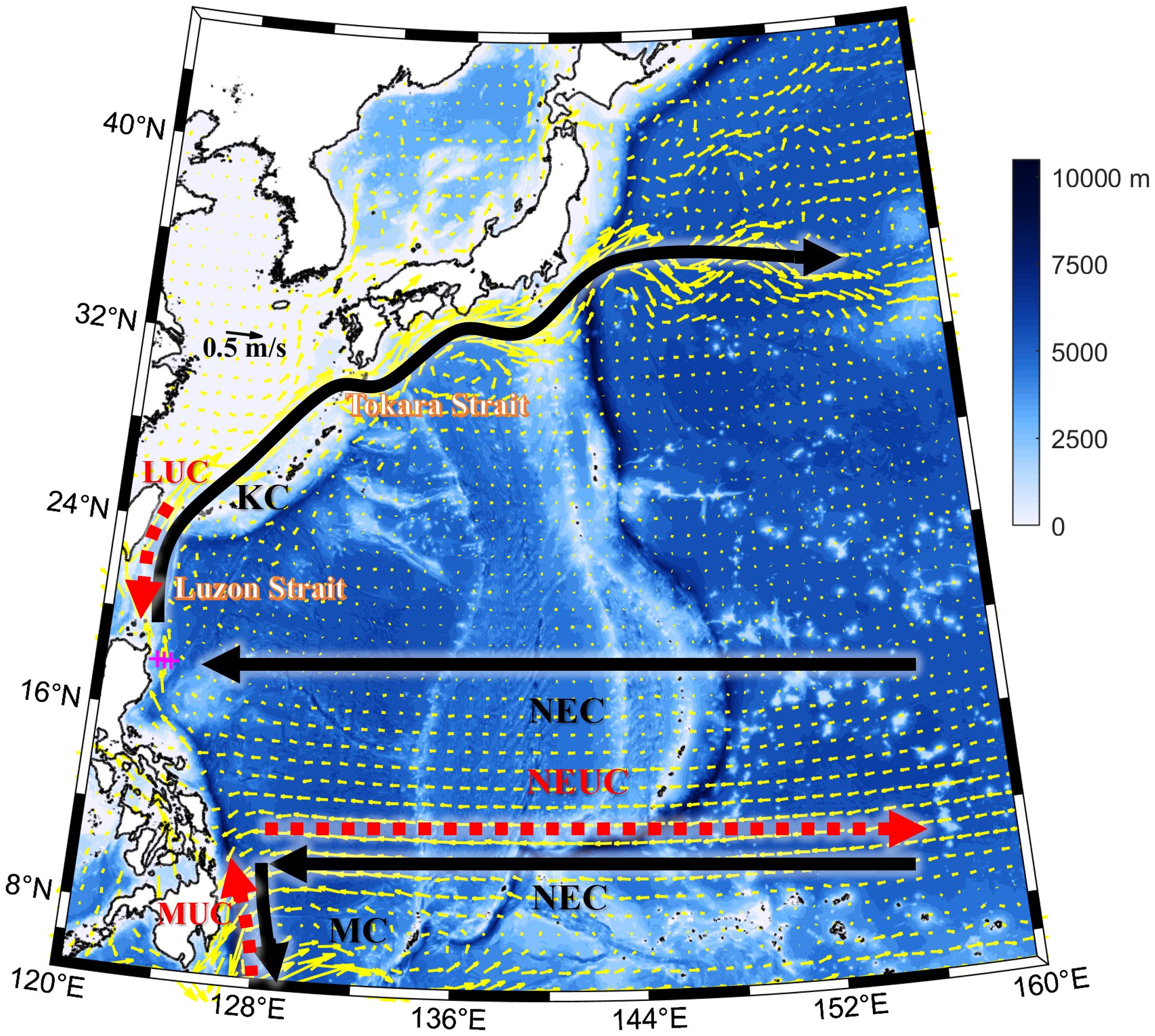
Figure 1. Bathymetry and current patterns in the Western Pacific Ocean. The background mean geostrophic current vectors (1993-2019, from Copernicus Marine Service; https://marine.copernicus.eu/) are shown as yellow arrows. Major surface currents, including the North Equatorial Current (NEC), Kuroshio Current (KC), and Mindanao Current (MC), are schematically represented by black solid arrows. Subsurface undercurrents, including the North Equatorial Undercurrent (NEUC), Luzon Undercurrent (LUC), and Mindanao Undercurrent (MUC), are denoted by red dashed arrows. The mooring locations at 122.7°E, 123°E, and 123.3°E along 18°N are marked by magenta crosses. The Luzon Strait and Tokara Strait are labeled. Bathymetry data are from GEBCO (https://download.gebco.net/).

The KC, a powerful western boundary current of the North Pacific subtropical gyre, transports warm water northward along Luzon Island (Lien et al., 2015). A portion of the KC intrudes into the South China Sea (SCS) via the Luzon Strait (Wu and Chiang, 2007; Qu et al., 2009), while the remainder flows northeastward past Taiwan and along the Ryukyu Islands and Japan. Near 35°N–40°N, it transitions into the Kuroshio Extension (Qiu et al., 1991; Joyce et al., 2001; Nakano et al., 2013; Sasaki and Minobe, 2015). The KC plays a pivotal role in global climate regulation, marine ecosystems, and regional weather patterns (Kwon et al., 2010; Hu et al., 2015).

Characterized by high velocities (>1 m/s) and warm water masses, the KC exhibits complex spatiotemporal variability driven by atmospheric and oceanic interactions. Long-term trends in KC strength have been reported, but their sign and magnitude show regional dependence. Mooring observations from 2010–2012 at 18°N revealed an increasing trend in KC velocity, linked to upper-ocean responses to low-frequency wind forcing (Chen et al., 2015). In contrast, Liu et al. (2021) documented a weakening trend during the 1998–2013 global warming hiatus near the Tokara Strait, suggesting flow-path dependence. On decadal and interannual timescales, the KC transport and its pathway are subject to substantial variability, primarily forced by large-scale wind anomalies over the Pacific Ocean associated with climate modes like the Pacific Decadal Oscillation (PDO) and the El Niño–Southern Oscillation (ENSO) (e.g., Qiu and Chen, 2010; Qiu et al., 2017). These low-frequency variations can modulate the strength of the KC by influencing the NEC (e.g., Zhai and Hu, 2013; Zhai et al., 2013) and the position of its bifurcation (Zhai et al., 2014a), which ultimately determines the energy partition between the northward-flowing KC and the southward-flowing MC. The combined influence of local and remote winds on this interannual-to-decadal KC variability has been highlighted (Fan et al., 2025). The KC also displays pronounced intraseasonal variability (20–120 days), driven by cyclonic and anticyclonic eddies along its path (Kakinoki et al., 2008; Andres et al., 2017; Mensah et al., 2020; Yuan et al., 2024).

Seasonally, the KC typically peaks in transport during winter–summer and reaches a minimum in fall along 18°N (Qu et al., 1998; Lien et al., 2014). This well-established seasonal pattern is predominantly governed by the basin-wide wind forcing over the North Pacific. The strengthening of the KC from winter to summer is largely driven by the intensification of the basin-scale anticyclonic wind stress curl, which strengthens the North Pacific subtropical gyre. The autumn minimum, conversely, is associated with the weakening of this wind stress curl and the arrival of upwelling Rossby waves. These waves manifest as negative sea surface height anomalies (SSHa) at the western boundary in autumn, reducing the geostrophic transport through Sverdrup balance and western boundary current dynamics (e.g., Qiu and Lukas, 1996; Yaremchuk and Qu, 2004). While consensus exists on its fall weakening, the season of maximum strength remains debated. Recently, Wang et al. (2022) reported an atypical seasonal cycle in 2018, attributing it to intraseasonal signals without addressing the roles of local wind and Rossby waves—key drivers of seasonal variability in wind-driven currents. This study investigates the atypical seasonal cycle of the KC in 2018, which was characterized by pronounced intraseasonal peaks during autumn, with a focus on quantifying the contributions of local wind and Rossby waves to this anomalous seasonal pattern through targeted model experiments.

This paper is organized as follows. The data and method are introduced in section 2. In section 3, the mean structure and atypical seasonal cycle of the KC in 2018 and then its dynamics are investigated. A conclusion is presented in section 4.

2 Data and method

2.1 Acoustic doppler current profilers data

To investigate the variability of the KC and LUC, three moorings were deployed at 122.7°E, 123°E, and 123.3°E along 18°N from January 2018 to May 2020. Each mooring was equipped with upward- and downward-looking 75 kHz ADCPs mounted at 450 m on the main float, configured with 60 bins (8 m per bin), providing a vertical observation range of 480 m. The combined velocity measurements from both instruments covered approximately 900 m of the water column. The observed velocity profile (~900 m) encompasses the core water masses of the KC system in this region. The KC is a surface-intensified flow, typically confined to the upper ~500 meters of the water column, characterized by its warm and saline water. Beneath the KC, the LUC, which carries colder, less saline water, flows equatorward. Our observational depth range therefore adequately captures the full vertical shear structure of the KC and the underlying LUC, allowing for a comprehensive analysis of their variability. Note that the downward-looking ADCP at 123°E/18°N malfunctioned. The raw data had vertical and temporal resolutions of 8 m and 1 hour, respectively. These raw data underwent a rigorous quality control procedure, during which data points were excluded if the recorded horizontal current velocity exceeded 2 m/s, the instrument tilt (pitch or roll) was greater than 18 degrees, or the percent good value fell below 80%. This process ensured the removal of spurious measurements caused by extreme events, mooring instability, or poor acoustic backscatter. Following quality control, the validated data were linearly interpolated onto a uniform vertical grid with 1-meter resolution and then averaged into daily means. Finally, due to strong beam echo interference, velocity measurements in the upper 50 m were excluded from the final analysis.

2.2 Global sea surface height data

The SSH dataset from the Copernicus Marine and Environment Monitoring Service (CMEMS) is an indispensable resource for researchers investigating oceanography. Its combination of satellite-based measurements, high-resolution data, and robust uncertainty estimates provides a comprehensive framework for advancing our understanding of global sea level dynamics. Daily SSH and geostrophic current data (0.25° × 0.25° resolution) from 1993–2019 were obtained from https://marine.copernicus.eu/. These satellite-derived datasets are widely used in oceanographic research due to their high resolution and robust uncertainty estimates.

2.3 HYbrid coordinate ocean model data

HYCOM is a widely used numerical ocean model that simulates ocean circulation and other physical processes. It uses a hybrid coordinate system, combining sigma levels (vertical coordinates based on pressure or density) with a time-dependent vertical grid to better represent the complex topography of the ocean. The model provides gridded outputs for temperature, salinity, currents, and surface height. In this study, HYCOM data with a horizontal resolution of 1/12° and 40 vertical levels were used, available at https://tds.hycom.org/thredds/catalog.html.

2.4 Ocean General circulation model for the earth simulator data

OFES, a high-resolution model developed by Japan Agency for Marine-Earth Science and Technology (JAMSTEC) and National Oceanic and Atmospheric Administration (NOAA)/Geophysical Fluid Dynamics Laboratory (GFDL), was used to analyze the relationship between local wind stress and the atypical seasonal cycle of the KC in 2018. The surface wind stress data, which are 3-day means, had a horizontal resolution of 0.1° and were sourced from http://apdrc.soest.hawaii.edu/dods/iprc_esc/OfES/. The wind stress curl from the OFES reanalysis was employed for the diagnostic analysis of the wind forcing mechanism, independent of the bulk algorithm used for the model forcing.

2.5 Regional ocean modeling system

The ROMS model is designed to simulate various oceanographic conditions like temperature, salinity, and currents over specific regions. It is characterized by high resolution, efficient computational requirements, and integration with other datasets or models. The model domain in the present study is in 15°N–20°N, 120°E-260°E, with a horizontal resolution of 10 km ×10 km and 15 vertical s-coordinate levels that are terrain-following and stretched to better resolve the upper ocean. The model’s initial conditions and lateral open boundary conditions were provided by the daily HYCOM reanalysis data (see Section 2.3 for data source details). A radiation condition was applied at the open boundaries, with nudging to the HYCOM data for temperature, salinity, and velocities to maintain consistency with the large-scale oceanic state.

The HYCOM global reanalysis data, used to provide lateral boundary conditions for the ROMS model, were quantitatively validated against in-situ mooring observations at 122.7°E, 18°N to ensure their reliability in the study region. The validation period was set from 25 January to 31 December 2018 to align with the specific focus of this paper, which investigates the atypical seasonal cycle of that year. The time series from both datasets were low-pass filtered to retain synoptic and lower-frequency signals. Statistical comparison based on the resulting 341 concurrent data points revealed a highly significant positive correlation (R = 0.59, p < 0.001), a negligible mean bias of 0.0039 m/s, and a root-mean-square error of 0.3240 m/s. These results demonstrate that the HYCOM data accurately capture the temporal evolution and mean state of the currents, providing high-confidence boundary forcing for our regional simulations.

Different wind products were employed for the model forcing and diagnostic analysis based on their respective strengths. The ROMS simulations were forced with hourly 10-m wind fields from the fifth generation of the European Centre for Medium-Range Weather Forecasts (ECMWF) atmospheric reanalysis (ERA5), for its high temporal (hourly) resolution, which is crucial for accurately capturing the diurnal cycle and high-frequency synoptic events that can influence ocean mixing and dynamics.

For the diagnostic analysis of wind stress curl in Section 3.4, we utilized the OFES product. Although it has a coarser temporal resolution (3-day means), OFES provides directly calculated wind stress curl fields that are dynamically consistent and well-validated for oceanographic studies. In contrast, deriving accurate wind stress curl from ERA5 would require additional processing and scaling, introducing potential uncertainties. The choice of each product was therefore optimized for its specific application.

3 Results

3.1 Mean structure of the KC

The mean meridional velocities from mooring observations (January 2018–May 2020) and HYCOM data (January 2015–May 2019) are shown in Figure 2. In this study, positive values denote eastward (u) and northward (v) velocities in all data processing and figures. Both datasets exhibit consistent spatial patterns across the three mooring stations (122.7°E, 123°E, and 123.3°E). The KC’s maximum velocities are concentrated in the upper 150 m, with mooring-recorded peaks of 72.4 cm/s (63 m depth), 40.6 cm/s (62 m), and 19.5 cm/s (115 m) at each station, respectively. HYCOM simulations show similar trends but with surface-intensified maxima (60.63 cm/s, 38.34 cm/s, and 22.88 cm/s). The westward intensification of the KC, with the maximum mean velocity occurring at the westernmost mooring (122.7°E), clearly indicates that its core lies further west. This finding is conclusively corroborated by independent observations. Satellite altimetry places the core near 122.625°E/18.125°N (Wang et al., 2022), while direct PIES measurements provide the most precise location, showing the annual-mean Kuroshio axis is at 122.43°E, within a narrow range of 122.35°E to 122.52°E at this latitude (Lien et al., 2014). Below 500 m, the LUC is observed only at the 122.7°E/18°N mooring.

Figure 2

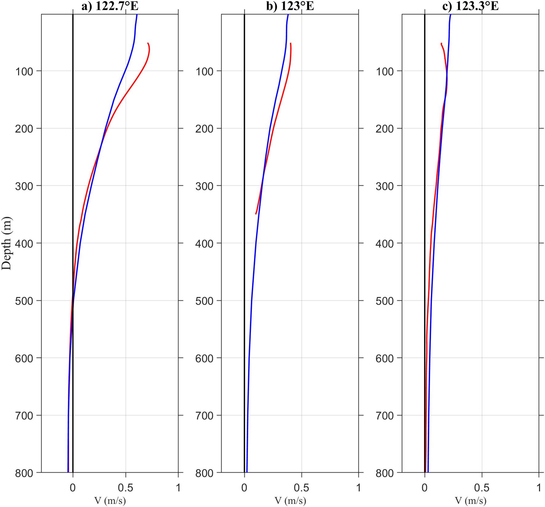
Figure 2. Mean meridional velocities from mooring observations (red lines; January 2018–May 2020) and HYCOM data (blue lines; January 2015–December 2019) at (a) 122.7°E, (b) 123°E, and (c) 123.3°E along 18°N. Black line indicates zero velocity (units: m s^-¹).

3.2 Seasonal variability of the KC

Time series from the moorings (Figure 3) reveal coherent phase but declining magnitude eastward from 122.7°E to 123.3°E. In 2019, the KC showed typical seasonal behavior, being relatively strong in winter–summer and weakest in autumn, consistent with prior studies (Qiu and Lukas, 1996; Yaremchuk and Qu, 2004). In contrast, 2018 showed an atypical cycle dominated by two distinct intraseasonal velocity peaks in late September and early November, which collectively altered the typical seasonal evolution of the current (e.g., Lien et al., 2014; Qiu and Lukas, 1996).

Figure 3

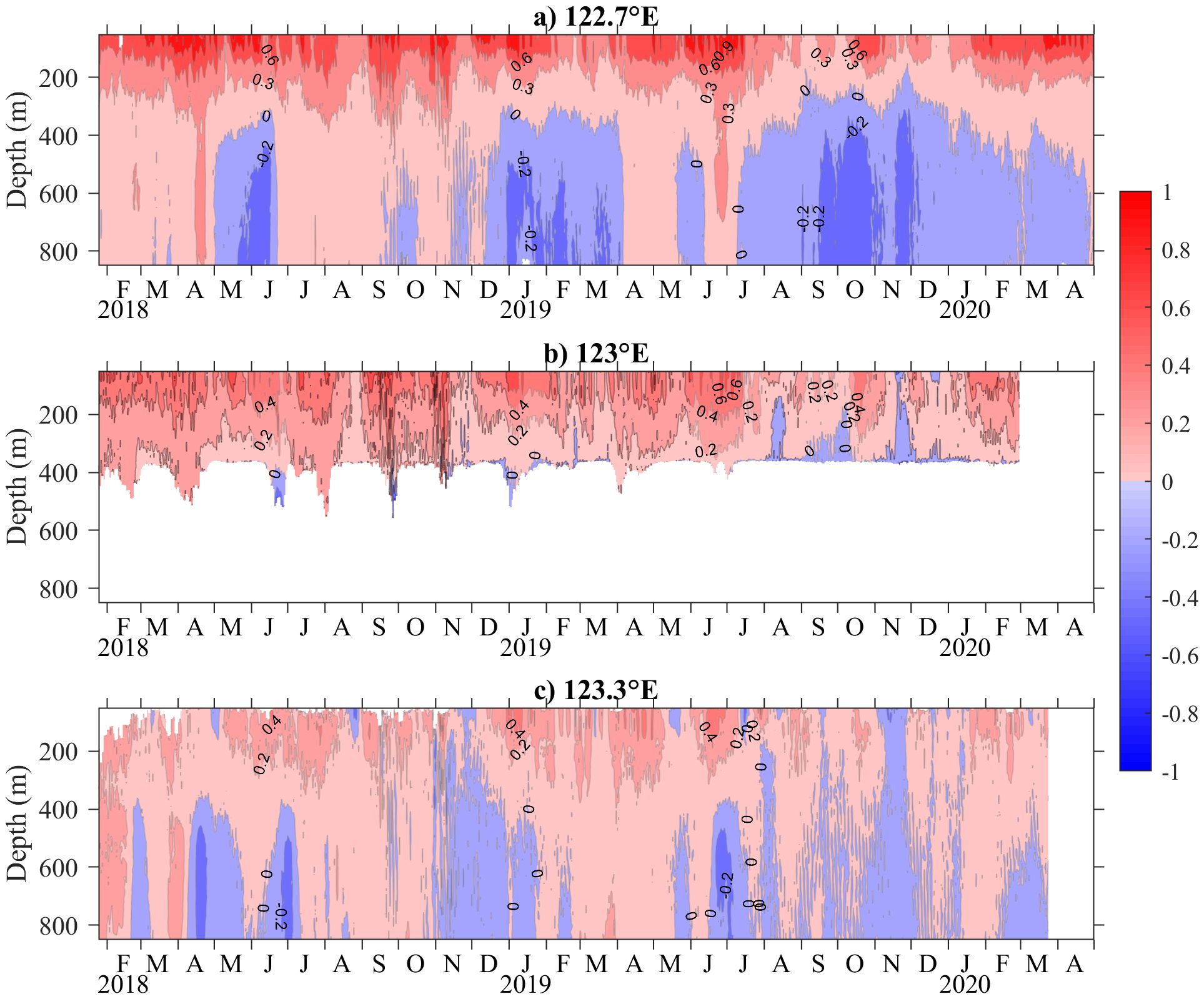
Figure 3. Meridional velocities from ADCP measurements at (a) 122.7°E, (b) 123°E, and (c) 123.3°E along 18°N (units: m s^-¹).

The mooring observations indicate that the anomalous seasonal cycle in 2018 was dominated by intraseasonal intensification events. A quantitative spectral analysis of these records, as detailed in our previous study (Wang et al., 2022), revealed that the energy of the 50–60 day intraseasonal band in the upper 350 m was significantly stronger in 2018 than in 2019 at all three mooring stations. This interannual difference in intraseasonal energy levels provides a quantitative measure of the unique character of the 2018 time series shown in Figure 3. Furthermore, the energy of these signals attenuated from west to east, indicating that the intraseasonal forcing was strongest near the core of the KC, which is located west of the mooring array.

The mooring data, while providing high-resolution temporal and vertical variability, are sporadic in space and cannot directly resolve the larger spatial context of the KC, such as zonal path shifting. Furthermore, it is difficult to derive the exact seasonal cycle and discuss its dynamics from a short, discontinuous record alone. To contextualize these point observations and verify their representativeness, we compared them with satellite and HYCOM data, which show similar trends during the study period (Figure 4). The monthly mean geostrophic velocity anomalies (Figures 5a-c) place the observations within a long-term climatological framework, confirming the atypical autumn strength in 2018.

Figure 4

Figure 4. Surface meridional velocity anomalies in 2018 from ADCPs (black solid line), satellite altimetry (green solid line), HYCOM (blue dashed line), and ROMS (red dashed line) at (a) 122.7°E, (b) 123°E, and (c) 123.3°E along 18°N (units: m s^-¹).

Figure 5

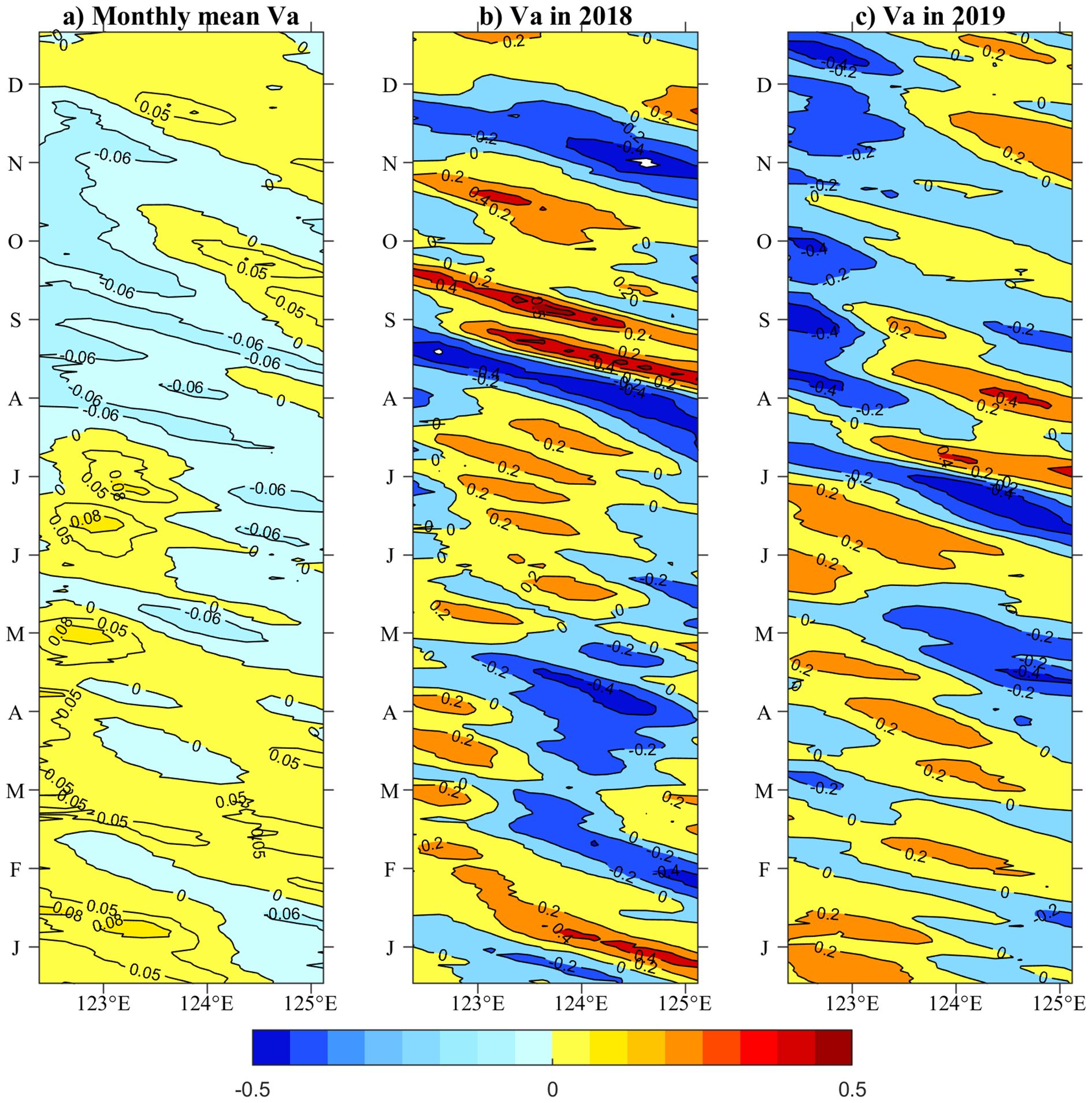
Figure 5. Meridional velocity anomalies along 18°N from satellite data in (a) monthly climatology, (b) 2018, and (c) 2019 (units: m s^-¹).

To further explore the spatial context, we examined the high-resolution HYCOM reanalysis. The analysis indicates that the seasonal velocity variations recorded at the mooring array are primarily linked to changes in the current’s intensity rather than a major zonal migration of its core. The core of the KC, as identified by the maximum velocity axis in HYCOM, remains west of the westernmost mooring (122.7°E) throughout the year (Figure 2). This supports the interpretation that the moorings are sampling the main flow of the KC, and that the observed seasonal signal is a reliable indicator of the integrated transport variability of the KC mainstream at this latitude.

3.3 Relative contribution from local wind and Rossby waves

The agreement between the mooring and satellite data indicates that the KC could be considered as a geostrophic current. In other words, the two peaks in late September and early November are attributed to the variability of SSH. The seasonal cycle of monthly mean sea surface height anomaly (SSHa) and the SSHa in 2018 and 2019 along 18°N are shown in Figures 6a, b and c, respectively. In Figure 6a, the SSHa is generally monotonic increasing in the first half of the year to a July maximum. In the second half of the year, it is almost monotonic decreasing. In addition, the seasonal phase generally delays towards west, resulting in the gradient of SSHa is almost positive/negative in the first/second half of the year except in winter, explaining the KC’s typical autumn minimum through geostrophic balance. While 2019 and early 2018 followed this typical cycle (Figures 6b,c), autumn 2018 showed an anomalous double-peak structure in SSHa that disrupted the expected seasonal decline, corresponding to the observed KC velocity maxima.

Figure 6

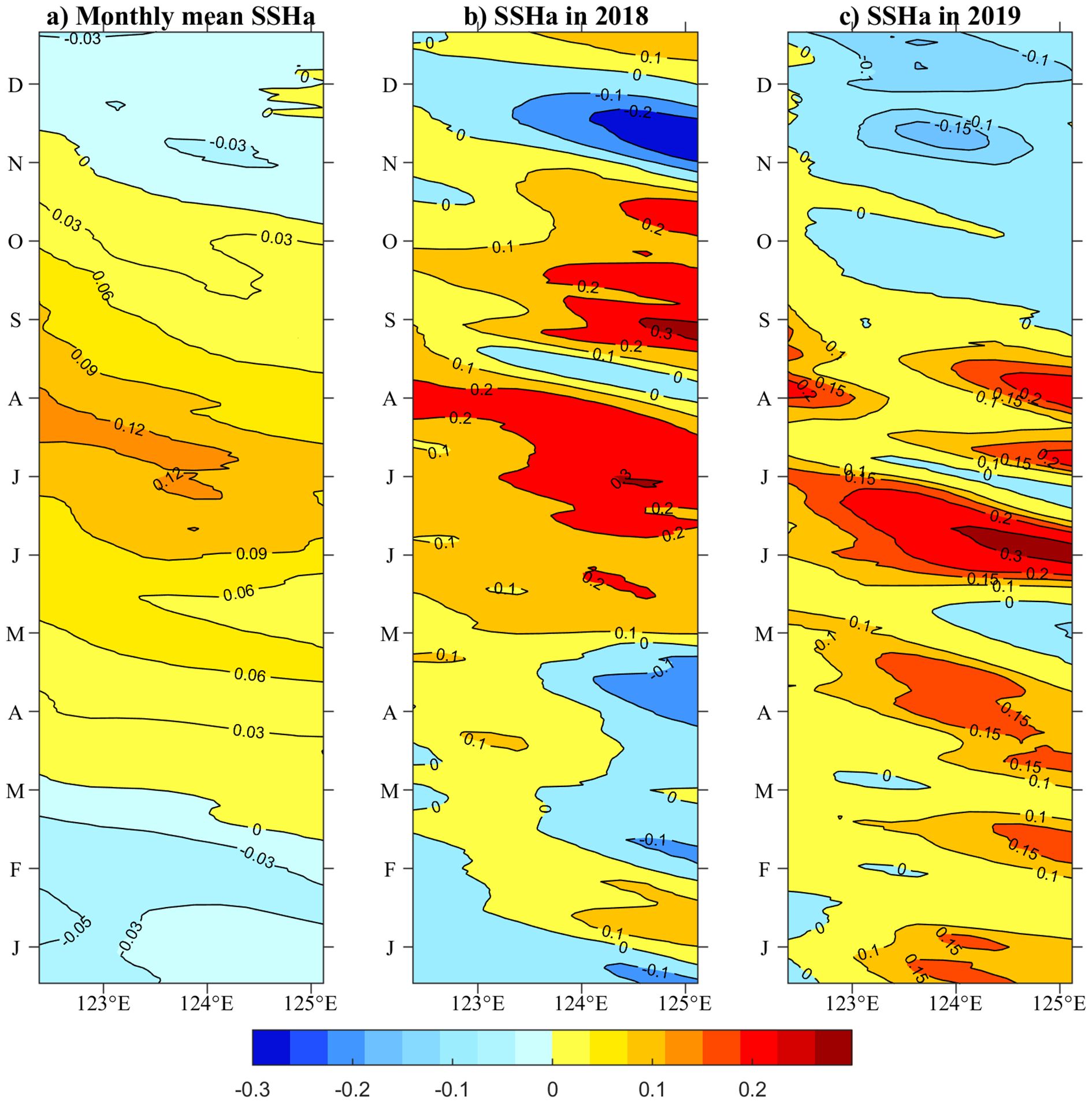
Figure 6. Satellite-derived SSHa along 18°N in (a) monthly climatology, (b) 2018, and (c) 2019 (units: m).

Previous work (Wang et al., 2022) identified enhanced 50–60 day intraseasonal variability in the upper ocean during 2018 compared to 2019 at our mooring stations, potentially linked to the observed autumn double-peak structure. However, the underlying dynamical mechanisms remained unquantified. In this paper, the dynamics of the atypical seasonal variability of the KC in 2018 is discussed associated with the local wind and Rossby waves, which are the key factors in the wind-driven ocean circulations and well demonstrated by the linearized reduced-gravity equation as follows (e.g., McCreary, 1981; Yan et al., 2014).

$\begin{array}{ll}\frac{\partial h}{\partial t}-(\frac{\beta c^2}{f^2})\frac{\partial h}{\partial x}=-\frac{1}{{\rho }_0}\nabla \times (\frac{\overrightarrow{\tau }}{f})& (1)\end{array}$

where $h(x,y,t)$ denotes the height deviation from the mean upper layer thickness $H_0$, $f$ is the Coriolis parameter, and $\beta =\frac{\partial f}{\partial y}$. $c=\sqrt{g^{\prime }{H}_0}$ is the internal wave speed, and $g^{\prime }=\frac{\text{Δ}\rho }{{\rho }_0}g$ is the reduced gravity, where ${\rho }_0$ and $\text{Δ}\rho$ represent the seawater density in the upper layer and the density difference between two layers, respectively. In the right hand, $\overrightarrow{\tau }$ is the surface wind stress.

Local wind significantly influences SSHa variability through Ekman pumping. A positive (negative) wind stress curl anomaly generates a corresponding negative (positive) SSHa. In the North Pacific Ocean, the seasonal phase of wind stress curl is largely latitudinally uniform, except near the western boundary (figure not shown), which may drive distinctive seasonal variability of the KC. The SSHa induced by local wind propagates westward via Rossby waves (Chelton and Schlax, 1996). Due to varying propagation distances, the signal arrives at the western boundary with phase differences. There, the SSHa can be interpreted as the superposition of wind forcing effects across the same latitude in the North Pacific Ocean. In other words, the SSHa at the western boundary reflects the zonal integration of both local and remote influences. Notably, Rossby wave propagation speed decreases with increasing latitude, resulting in a westward delay in the seasonal phase of SSHa along 18°N (Figure 6).

The ROMS is a three-dimensional, free-surface, terrain-following numerical model. Prior to the sensitivity experiments, we evaluated the model’s performance in representing the current characteristics of the study region. A comparison of the surface meridional velocities from the ROMS control run with in situ mooring observations, satellite data, and HYCOM outputs at the three mooring stations is presented in Figure 4.

A detailed intercomparison of the four datasets offers valuable insights into their characteristics. The model demonstrates a strong agreement with the independent datasets in capturing the timing of the major variability events, including the atypical double-peak in autumn 2018. The mooring and satellite altimetry data show strong agreement on seasonal and intraseasonal timescales, although the satellite product, as expected, attenuates the highest-frequency variability resolved by the hourly mooring records.

The model-data comparison during the two autumn 2018 peak periods reveals a nuanced picture. For the first peak, the ROMS control run shows excellent agreement with the mooring observations, accurately capturing both its timing and amplitude. For the second peak, however, ROMS, along with the HYCOM reanalysis, exhibits a stronger northward velocity anomaly than the in situ data, although the overestimation in ROMS is notably smaller than that in HYCOM. This systematic yet differential bias suggests that while the atmospheric forcing fields common to both models may overestimate the intensity of the wind stress curl anomaly that drove the second event, the ROMS configuration, likely due to its specific physics parameterizations, simulates the ocean’s response to this forcing more accurately than HYCOM.

The inclusion of the HYCOM reanalysis provides a broader context. The fact that both models show a similar bias for the second peak, albeit to different degrees, indicates that the challenge in fully capturing this event’s intensity is not a unique artifact of our specific ROMS configuration but is related to a broader issue, potentially in the common atmospheric forcing. Crucially, the superior performance of ROMS in mitigating this bias, especially its perfect simulation of the first peak, demonstrates that the core physics of the wind-ocean coupling are well represented in our model setup. This performance validates its use for process-oriented diagnosis.

To quantitatively evaluate the model’s performance in capturing the temporal evolution, we calculated the correlation coefficient (R), root-mean-square error (RMSE), and bias against the in-situ mooring observations, which provide continuous, point-on-location measurements ideal for time-series validation. At the representative 122.7°E/18°N site, the ROMS simulation of the low-pass filtered surface meridional velocity anomaly shows a statistically significant correlation with the mooring data (R = 0.52, p < 0.001), with an RMSE of 0.26 m/s and a negligible bias of +0.003 m/s. This quantitative assessment confirms that the model successfully captures the primary low-frequency variability observed. A similarly robust agreement was found between ROMS and the data-assimilative HYCOM reanalysis at this location (R = 0.87, RMSE = 0.29 m/s, Bias = −0.002 m/s), lending further confidence. The statistical metrics at the other mooring sites, while slightly varying in magnitude due to data coverage, consistently showed significant correlations and low errors, thereby rigorously validating the model’s reliability for the subsequent dynamical analysis.

To isolate the relative contributions of wind forcing and Rossby waves to the atypical seasonal cycle of the KC in 2018, we conducted two sensitivity experiments using ROMS. In Experiment 1 (EXP1), winds east of 125°E were held constant at 2018 climatological values, and winds west of 125°E were held constant at 2018 climatological values in Experiment 2 (EXP2). Figure 7 shows that the seasonal cycle from the ROMS control run (which, as demonstrated in Figure 4, aligns closely with HYCOM, satellite and mooring observations) is largely reproduced by EXP1. This indicates that winds west of 125°E dominate the seasonal variability of the KC along 18°N. In contrast, EXP2 eliminated the two autumn 2018 peaks, suggesting that westward-propagating Rossby waves were not a key driver of the atypical variability that year. A detailed quantitative comparison between the sensitivity experiments and the control run reveals an informative pattern. At the core station (122.7°E), EXP1 (local wind) exhibits the highest correlation (R = 0.79), significantly outperforming EXP2 (remote Rossby waves, R = 0.69). A complementary analysis of the RMSE and bias further substantiates this finding: EXP1 yields a lower RMSE and a smaller systematic bias compared to EXP2, indicating a superior overall agreement with the observed amplitude and mean state of the Kuroshio transport. However, the correlation of EXP1 decreases eastward with distance from the local wind forcing source, while EXP2 maintains a stable and spatially uniform correlation across the mooring array. This statistical pattern is consistent with the distinct physical nature of each forcing: the “near-field effect” of local winds versus the large-scale, coherent background modulation expected from remote Rossby waves. The central aim of this study, however, is to diagnose the drivers of the atypical 2018 seasonal cycle, which was defined by two distinct intraseasonal peaks in autumn. Therefore, the capability to reproduce these specific diagnostic events serves as the ultimate criterion for assessment. By this crucial metric, the decisive role of EXP1 becomes unequivocal, as it alone successfully captures the timing and amplitude of both intensification events. In contrast, the temporal evolution simulated by EXP2 is overly smooth and fails entirely to reproduce the defining peaks of the anomaly, a key contributor to its higher RMSE. Consequently, the moderately high correlations in EXP2 likely reflect its skill in simulating the large-scale, low-frequency background variability, which was not the physical driver of the specific anomalous events. In summary, local wind forcing west of 125°E was the indispensable and dominant driver of the atypical 2018 seasonal cycle, whereas remotely generated Rossby waves provided only a spatially coherent background modulation, playing a negligible role in generating the targeted anomaly. In fact, the eastern boundary of local wind forcing was initially set at 140°E before two experiments, yielding results consistent with those shown in Figure 7. Through iterative adjustments, we shifted this boundary westward in the model until reaching 125°E. The final domain for local wind effects was thus defined as the region bounded by 120°E–125°E and 15°N–20°N.

Figure 7

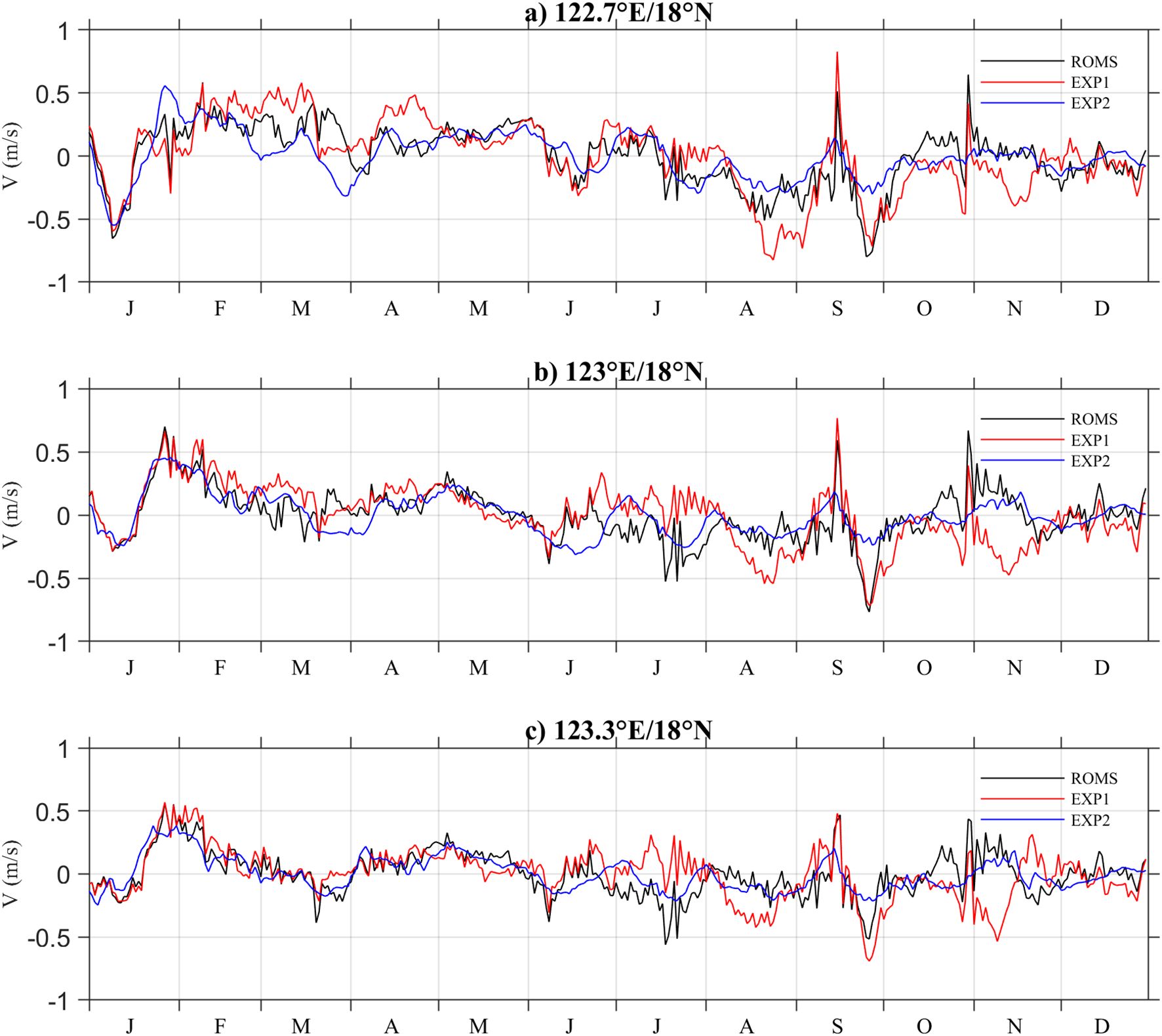
Figure 7. Surface meridional velocity anomalies in 2018 from ROMS simulations: control run (black line), Experiment 1 (red line), and Experiment 2 (blue line) at (a) 122.7°E, (b) 123°E, and (c) 123.3°E along 18°N (units: m s^-¹).

3.4 Dynamics of atypical seasonal variability of the KC in 2018

The sensitivity experiments in Section 3.3 have pinpointed the local wind as the key driver. To diagnose the detailed physical process through which this wind forcing operates to generate the specific oceanic anomalies observed in 2018 (and whose absence explains the quiet conditions in 2019), we now turn to a direct analysis of the satellite and wind field data. This observation-based diagnostic approach allows us to visualize the spatial structure and synoptic-scale evolution of the forcing and response, providing a direct link between the atmospheric anomaly and the oceanic current. The ROMS simulations, having already demonstrated the causal relationship, provide the foundation that justifies this closer physical inspection of the observational record.

The surface forcing for the ROMS numerical experiments was derived from the ERA5 reanalysis. It is important to note that ERA5 provides 10-meter wind velocity components but does not output a surface wind stress field directly. Therefore, the wind stress required to force the ocean model was calculated from these winds using established bulk algorithms. The derivation of wind stress from 10-meter winds is a recognized source of uncertainty in oceanographic modeling. This process involves parameterizations for the drag coefficient and atmospheric stability, where different algorithmic choices can lead to quantitatively and sometimes qualitatively different wind stress estimates. To enhance the robustness and objectivity of our diagnostic analysis on wind forcing, we utilized the wind stress field from the OFES reanalysis. The OFES product provides a direct, dynamically consistent, and ocean-model-oriented estimate of wind stress. This strategic choice allows our mechanistic conclusions regarding the dominant physical processes to be based on a forcing field that is independent of the specific bulk algorithm used in our model setup. This approach is a common practice in physical oceanography to isolate diagnostic results from potential biases inherent in the wind stress calculation step.

The analysis of the daily evolution of SSHa (from satellite data) and wind stress curl anomalies (from OFES data) at 3-day intervals reveals the following physical evolution. For the first peak period (22 September to 1 October, 2018), the physical evolution is shown in Figures 8a-d and 9a-d. A strong positive SSHa emerged near 125°E/18.5°N on 22 September (Figure 8a) and propagated westward, reaching 124.4°E by 1 October. As this positive SSHa was located east of the mooring stations, it generated a northward geostrophic velocity anomaly through geostrophic balance, consistent with the first observed KC peak.

Figure 8

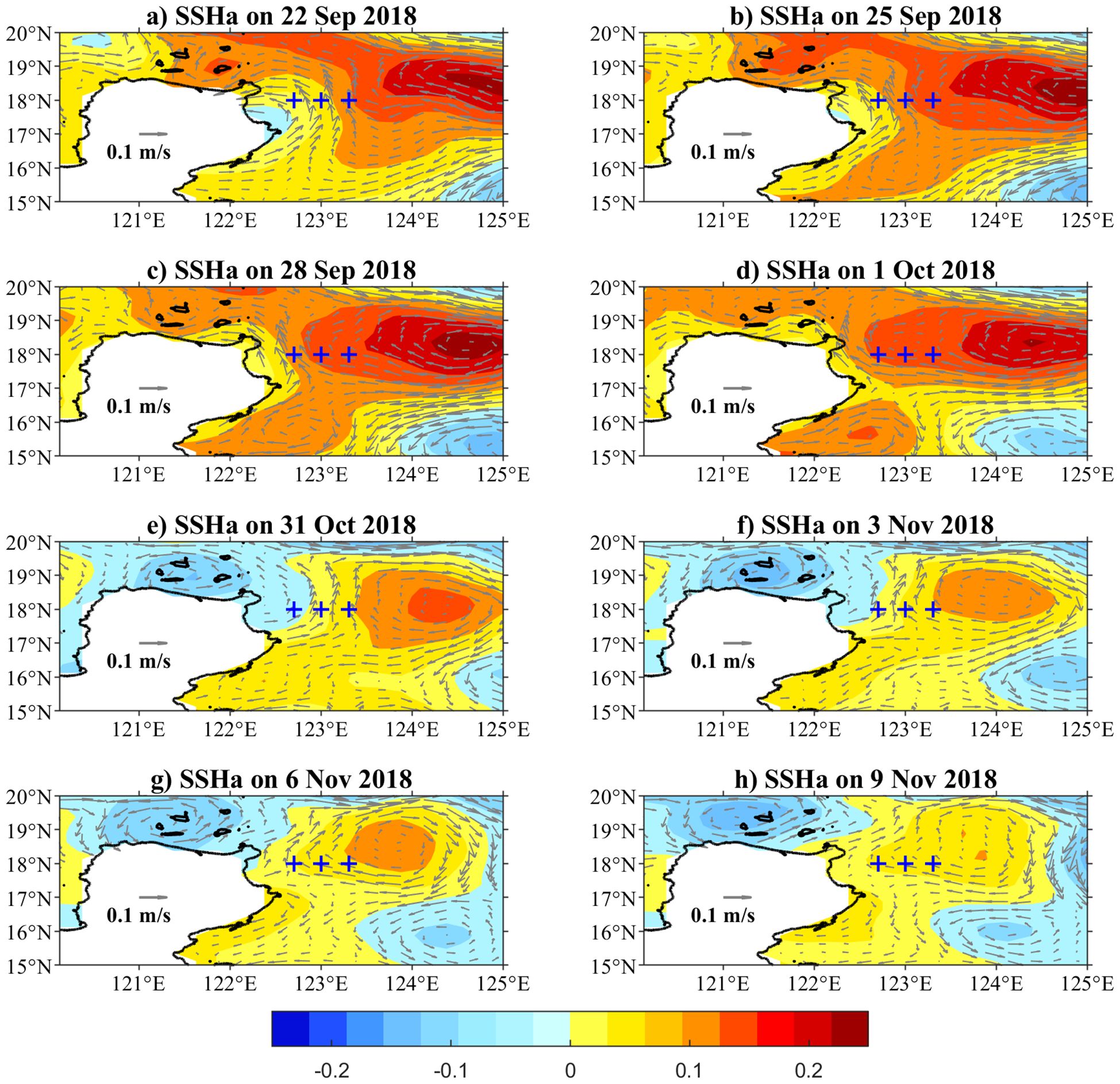
Figure 8. Satellite SSHa and geostrophic currents in the study region (120°E–125°E, 15°N–20°N) during 2018: (a–d) first peak period (22 September–1 October) and (e–h) second peak period (31 October–9 November) (units: m). Three mooring stations are depicted by blue crosses.

Figure 9

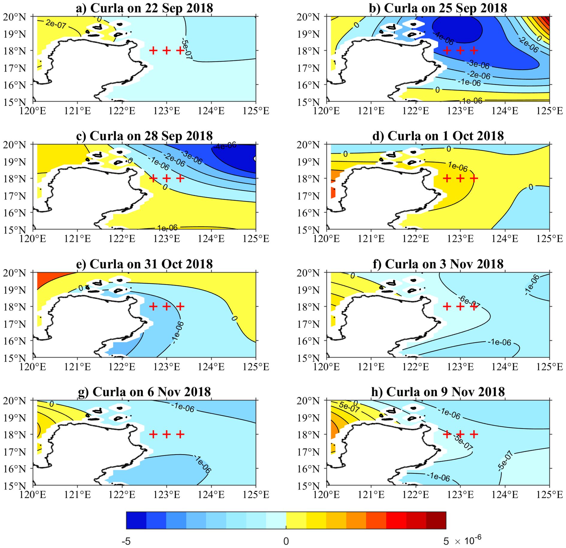
Figure 9. Wind stress curl anomalies (from OFES data) in the study region during 2018: (a–d) first peak period and (e–h) second peak period (units: 10^-6 N m^-³). Three mooring stations are represented by red crosses.

This oceanic response was driven by the atmospheric forcing. The corresponding wind stress curl anomaly east of the mooring stations was predominantly negative during this period (e.g., Figures 9a-c), which induces Ekman suction and raises sea level, thus generating and maintaining the observed positive SSHa. On 28 September, the extreme values of both the negative wind stress curl and the positive SSHa were concentrated near 18°N–19°N along 125°E (Figures 8c, 9c), coinciding with the KC maximum.

A key aspect of the wind-ocean coupling is the integration of the wind forcing over time, as expressed in Equation 1. This process is clearly demonstrated by the evolution at the end of the period. On 1 October (Figure 9d), the wind stress curl anomaly had shifted to positive, which would act to depress sea level. However, the SSHa remained positive (although weakened, Figure 8d) due to the accumulated effect of the prior persistent negative wind curl forcing. This hysteresis illustrates that the ocean’s response integrates rapid atmospheric variations, resulting in a more slowly varying SSHa field.

A similar mechanism operated during the second peak period (31 October-9 November 2018), albeit with a weaker amplitude. A persistent negative wind stress curl anomaly east of the mooring stations (Figures 9e-h) generated a corresponding positive SSHa (Figures 8e-h), which in turn produced the second observed KC peak through geostrophic balance.

The quantitative relationship between the forcing and the response is clearly evident as follows. The weaker intensity of the wind stress curl anomaly during this period corresponded to a smaller magnitude of the SSHa compared to the first event. This direct scaling further confirms the dominance of local wind forcing in generating these events.

Although the SSHa magnitude was smaller, the resulting KC velocity anomaly was comparable to the first event. We attribute this to two factors. First, the geostrophic velocity is a function of the gradient of SSHa, not its absolute magnitude. A compact, sharply defined SSHa feature can generate a strong velocity jet even if its peak amplitude is moderate. Second, the peak SSHa during the second event was located closer to the mooring array (Figures 8e-h), placing the moorings directly within a region of strong horizontal shear, thereby capturing a stronger velocity signal. After 9 November, the wind stress curl turned positive (figure not shown), leading to the eventual disappearance of the peak.

In stark contrast, the oceanic conditions during the climatologically equivalent periods in 2019 (23 September–2 October and 1–10 November, offset by one day from 2018 due to the 3-day temporal resolution of the OFES data) were fundamentally different. Satellite data reveal a persistent negative SSHa east of the moorings during these periods (Figure 10), which would generate a southward geostrophic velocity anomaly.

Figure 10

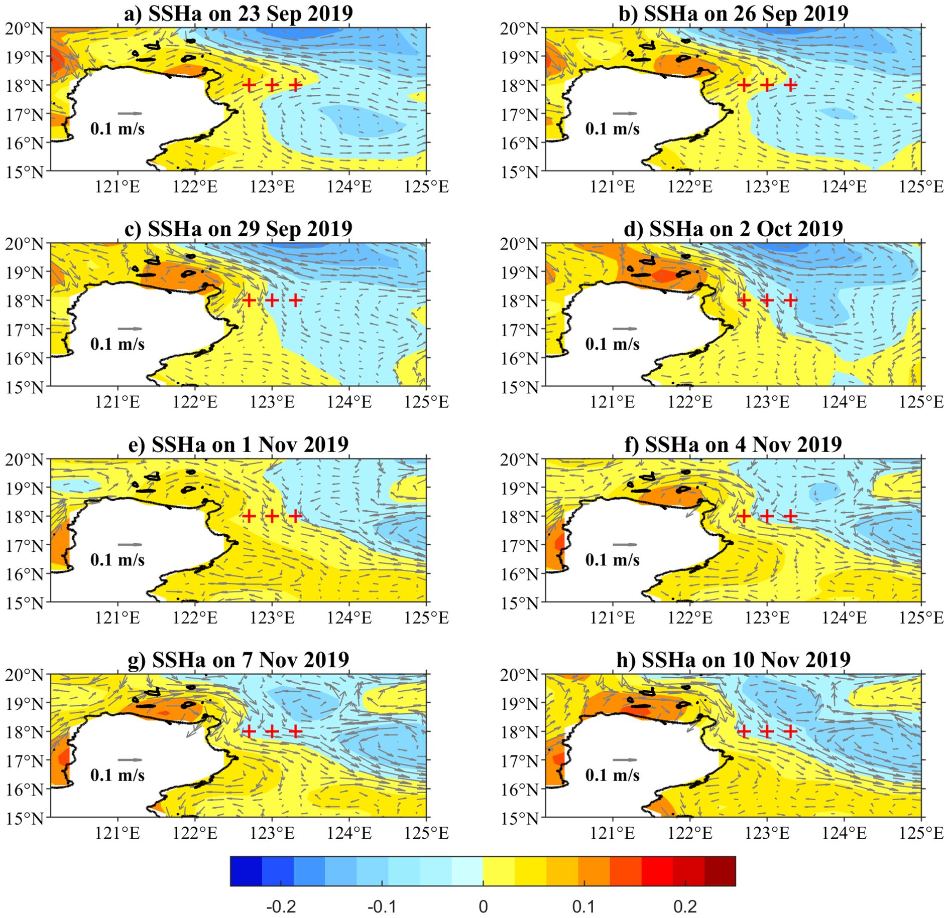
Figure 10. Satellite SSHa and geostrophic currents in the study region during 2019: (a–d) first period (23 September–2 October) and (e–h) second period (1–10 November) (units: m). Three mooring stations are denoted by red crosses.

This oceanic state was forced by the atmospheric conditions. A predominantly positive wind stress curl anomaly dominated the region (Figures 11a-c, e-h, with a brief negative anomaly occurring only on 2 October in Figure 11d). This opposite wind forcing pattern induces Ekman downwelling, which suppresses sea level and is consistent with the observed negative SSHa. The prevailing positive wind stress curl anomaly therefore created the conditions that suppressed northward flow, explaining the absence of autumn peaks in 2019.

Figure 11

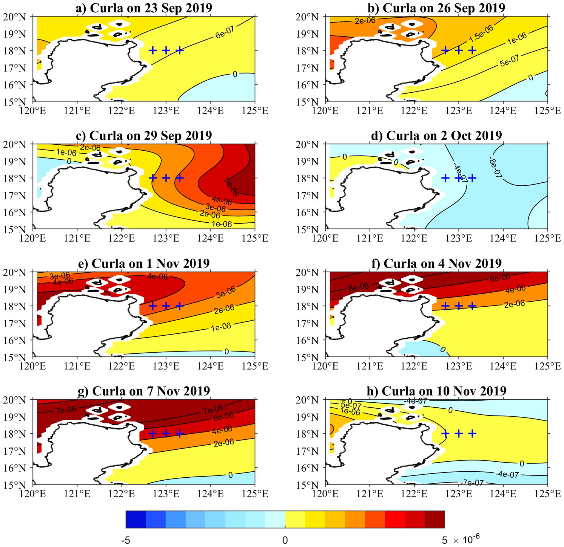
Figure 11. Wind stress curl anomalies (from OFES data) in the study region during 2019: (a–d) first period and (e–h) second period (units: 10^-6 N m^-³). Three mooring stations are marked by blue crosses.

4 Conclusions

Utilizing three moorings deployed at 122.7°E, 123°E and 123.3°E along 18°N, the mean structure and seasonal variability of the KC are investigated. The maximum of the mean KC on three mooring stations are all concentrated in the upper 150 m. The mean KC become larger towards the west, suggesting the core of the KC is located west of the 122.7°E along 18°N, which is consistent with the results from previous research (Lien et al., 2014; Wang et al., 2022).

The KC exhibited typical climatological seasonality in 2019, with relatively strong transport in winter, spring, and summer, and minimum in autumn. However, 2018 showed an atypical autumn season characterized by a double-peak structure in the current’s transport. While the individual peaks were intraseasonal in duration, their occurrence and timing resulted from an anomalous seasonal-scale wind forcing pattern over the key region (120°E–125°E, 15°N–20°N), as demonstrated by our ROMS model experiments. Thus, the intraseasonal events were the manifestation of a larger-scale, seasonally-atypical driving mechanism.

The robustness of this wind-driven mechanism is further confirmed by our sensitivity experiment. In EXP2, the removal of the anomalous local wind forcing west of 125°E effectively synthesized a typical Kuroshio state within the same model framework. The resultant disappearance of the double-peak intensification and the reversion to a canonical seasonal cycle demonstrate that the local wind dynamics are necessary for generating the atypical event. This confirms that the identified local mechanism is not an artifact of the specific year but a fundamental process whose outcome is determined by the presence or absence of sustained, anomalous local wind stress curl.

Analysis of SSHa and wind stress curl anomalies reveals the physical mechanism as follows. During the 2018 peak periods (22 Sep–1 Oct and 31 Oct–9 Nov), persistent negative wind stress curl anomalies (except 1 October) generated positive SSH anomalies east of Luzon Island through integrated wind forcing, producing the two observed velocity peaks. Conversely, predominantly positive wind stress curl anomalies during equivalent 2019 periods (23 Sep–2 Oct and 1–10 Nov, except 2 October) created opposite conditions, explaining the absence of autumn peaks that year.

The anomalous acceleration events documented in this study contribute to a growing body of literature on the wind-driven modulation of the KC. The core mechanism, Ekman pumping driven by wind stress curl anomalies leading to geostrophic flow adjustments, is a fundamental process that operates across seasons. This study demonstrates that this mechanism is not limited to explaining the current’s weakening during strong winter monsoons (e.g., Lee et al., 2001; Qiu and Lukas, 1996), but is also the primary driver of its anomalous intensification, as was the case in autumn 2018. What makes our case distinct is the seasonal timing (autumn, typically a period of weakening) and the atmospheric origin (linked to a persistent anomaly in the regional wind field). This juxtaposition of a typical mechanism acting at an atypical time to produce an extreme event provides a deeper insight into the complex interplay between atmospheric variability and western boundary current dynamics.

Data availability statement

The original contributions presented in the study are included in the article/supplementary material. Further inquiries can be directed to the corresponding author.

Author contributions

FW: Conceptualization, Funding acquisition, Writing – original draft, Writing – review & editing. LZ: Investigation, Writing – review & editing. JF: Methodology, Writing – review & editing. QW: Data curation, Writing – review & editing. DH: Validation, Writing – review & editing.

Funding

The author(s) declare financial support was received for the research and/or publication of this article. This research was financially supported by Laoshan Laboratory (LSKJ202201601), the Strategic Priority Research Program of the Chinese Academy of Sciences (grant XDB42010105), and the National Key Research and Development Program of China (2020YFA0608801).

Acknowledgments

We express our sincere gratitude to all scientists and technicians on R/V Science and Science 3 for the deployment and retrieval of three moorings used in this work.

Conflict of interest

The authors declare that the research was conducted in the absence of any commercial or financial relationships that could be construed as a potential conflict of interest.

Generative AI statement

The author(s) declare that no Generative AI was used in the creation of this manuscript.

Any alternative text (alt text) provided alongside figures in this article has been generated by Frontiers with the support of artificial intelligence and reasonable efforts have been made to ensure accuracy, including review by the authors wherever possible. If you identify any issues, please contact us.

Publisher’s note

All claims expressed in this article are solely those of the authors and do not necessarily represent those of their affiliated organizations, or those of the publisher, the editors and the reviewers. Any product that may be evaluated in this article, or claim that may be made by its manufacturer, is not guaranteed or endorsed by the publisher.

References

Andres M., Mensah V., Jan S., Chang M.-H., Yang Y.-J., Lee C. M., et al. (2017). Downstream evolution of the Kuroshio’s time-varying transport and velocity structure. J. Geophys. Res. 122, 3519–3542. doi: 10.1002/2016JC012519

Crossref Full Text | Google Scholar

Chelton D. B. and Schlax M. G. (1996). Global observations of oceanic Rossby waves. Science 272, 234–238. doi: 10.1126/science.272.5259.234

Crossref Full Text | Google Scholar

Chen Z., Wu L., Qiu B., Li L., Hu D., Liu C., et al. (2015). Strengthening Kuroshio observed at its origin during November 2010 to October 2012. J. Geophys. Res. 120, 2460–2470. doi: 10.1002/2014JC010590

Crossref Full Text | Google Scholar

Fan M., Liu X., Liu T., and Chen D. (2025). The role of local wind stress curl in modulating Kuroshio Extension latitudinal variability. J. Geophys. Res. 130, e2024JC021742. doi: 10.1029/2024JC021742

Crossref Full Text | Google Scholar

Gordon A. L., Flament P., Villanoy C., and Centurioni L. (2014). The nascent kuroshio of lamon bay. J. Geophys. Res. 119, 4251–4263. doi: 10.1002/2014JC009882

Crossref Full Text | Google Scholar

Hu D. and Cui M. (1991). The western boundary current of the Pacific and its role in the climate. J. Oceanol. Limnol. 9, 1–14. doi: 10.1007/BF02849784

Crossref Full Text | Google Scholar

Hu S., Hu D., Guan C., Wang F., Zhang L., Wang F., et al. (2016). Interannual variability of the mindanao current/undercurrent in direct observations and numerical simulations. J. Phys. Oceanogr. 46, 483–499. doi: 10.1175/JPO-D-15-0092.1

Crossref Full Text | Google Scholar

Hu D., Hu S., Wu L., Li L., Zhang L., Diao X., et al. (2013). Direct measurements of the luzon undercurrent. J. Phys. Oceanogr. 43, 1417–1425. doi: 10.1175/JPO-D-12-0165.1

Crossref Full Text | Google Scholar

Hu D., Wu L., Cai W., Gupta A. S., Ganachaud A., Qiu B., et al. (2015). Pacific western boundary currents and their roles in climate. Nature. 522, 299–308. doi: 10.1038/nature14504

PubMed Abstract | Crossref Full Text | Google Scholar

Joyce T. M., Yasuda I., Hiroe Y., Komatsu K., Kawasaki K., and Bahr F. (2001). Mixing in the meandering Kuroshio Extension and the formation of North Pacific Intermediate Water. J. Geophys. Res. 106, 4397–4404. doi: 10.1029/2000JC000232

Crossref Full Text | Google Scholar

Kakinoki K., Imawaki S., Uchida H., Nakamura H., Ichikawa K., Umatani S.-I., et al. (2008). Variations of Kuroshio geostrophic transport south of Japan estimated from long-term IES observations. J. Oceanogr. 64, 373–384. doi: 10.1007/s10872-008-0030-4

Crossref Full Text | Google Scholar

Kashino Y., Ueki I., and Sasaki H. (2015). Ocean variability east of Mindanao: Mooring observations at 7°N, revisited. J. Geophys. Res. 120, 2540–2554. doi: 10.1002/2015JC010703

Crossref Full Text | Google Scholar

Kwon Y.-O., Alexander M. A., Bond N. A., Frankignoul C., Nakamura H., Qiu B., et al. (2010). Role of the Gulf Stream and Kuroshio–Oyashio systems in large-scale atmosphere–ocean interactions: A review. J. Climate. 23, 3249–3281. doi: 10.1175/2010JCLI3343.1

Crossref Full Text | Google Scholar

Lee T. N., Johns W. E., Liu C. T., Zhang D., Zantopp R., and Yang Y. (2001). Mean transport and seasonal cycle of the Kuroshio east of Taiwan with comparison to the Florida Current. J. Geophys. Res. 106, 22143–22158. doi: 10.1029/2000JC000535

Crossref Full Text | Google Scholar

Lien R. C., Ma B., Cheng Y. H., Ho C. R., Qiu B., Lee C. M., et al. (2014). Modulation of Kuroshio transport by mesoscale eddies at the Luzon Strait entrance. J. Geophys. Res. 119, 2129–2142. doi: 10.1002/2013JC009548

Crossref Full Text | Google Scholar

Lien R. C., Ma B., Lee C. M., Sanford T. B., Mensah V., Centurioni L. R., et al. (2015). The kuroshio and luzon undercurrent east of luzon island. Oceanography 28, 54–63. doi: 10.5670/oceanog.2015.81

Crossref Full Text | Google Scholar

Liu Z.-J., Zhu X.-H., Nakamura H., Nishina A., Wang M., and Zheng H. (2021). Comprehensive observational features for the Kuroshio transport decreasing trend during a recent global warming hiatus. Geophys. Res. Lett. 48, e2021GL094169. doi: 10.1029/2021GL094169

Crossref Full Text | Google Scholar

McCreary J. P. (1981). A linear stratified ocean model of the equatorial undercurrent. Philos. Trans. R. Soc London Ser. A 298, 603–635. doi: 10.1098/rsta.1981.0002

Crossref Full Text | Google Scholar

Mensah V., Jan S., Andres M., and Chang M.-H. (2020). Response of the Kuroshio east of Taiwan to mesoscale eddies and upstream variations. J. Oceanogr. 76, 271–288. doi: 10.1007/s10872-020-00544-8

Crossref Full Text | Google Scholar

Nakano H., Tsujino H., and Sakamoto K. (2013). Tracer transport in cold-core rings pinched off from the Kuroshio Extension in an eddy-resolving ocean general circulation model. J. Geophys. Res. 118, 5461–5488. doi: 10.1002/jgrc.20375

Crossref Full Text | Google Scholar

Nitani H. (1972). “Beginning of the kuroshio,” in Kuroshio: Its physical aspects. Eds. Stommel H. and Yoshida K. (Univ. of Wash. Press, Seattle), 129–163.

Google Scholar

Qiu B. and Chen S. (2010). Interannual-to-decadal variability in the bifurcation of the North Equatorial Current off the Philippines. J. Phys. Oceanogr. 40, 2525–2538. doi: 10.1175/2010JPO4462.1

Crossref Full Text | Google Scholar

Qiu B., Chen S., and Schneider N. (2017). Dynamical links between the decadal variability of the Oyashio and Kuroshio Extensions. J. Climate. 30, 9591–9605. doi: 10.1175/JCLI-D-17-0397.1

Crossref Full Text | Google Scholar

Qiu B., Chen S., Schneider N., and Taguchi B. (2014). A coupled decadal prediction of the dynamic state of the Kuroshio Extension system. J. Climate. 27, 1751–1764. doi: 10.1175/JCLI-D-13-00318.1

Crossref Full Text | Google Scholar

Qiu B., Kelly K. A., and Joyce T. M. (1991). Mean flow and variability in the Kuroshio Extension from Geosat altimetry data. J. Geophys. Res. 96, 18491–18507. doi: 10.1029/91JC01834

Crossref Full Text | Google Scholar

Qiu B. and Lukas R. (1996). Seasonal and interannual variability of the north Equatorial Current, the Mindanao Current, and the Kuroshio along the Pacific western boundary. J. Geophys. Res. 101, 12315–12330. doi: 10.1029/95JC03204

Crossref Full Text | Google Scholar

Qiu B., Rudnick D. L., Chen S., and Kashino Y. (2013). Quasi-stationary North Equatorial Undercurrent jets across the tropical North Pacific Ocean. Geophys. Res. Lett. 40, 2183–2187. doi: 10.1002/grl.50394

Crossref Full Text | Google Scholar

Qu T., Chiang T.-L., Wu C.-R., Dutrieux P., and Hu D. (2012). Mindanao current/undercurrent in an eddy-resolving GCM. J. Geophys. Res. 117, C06026. doi: 10.1029/2011JC007838

Crossref Full Text | Google Scholar

Qu T., Kagimoto T., and Yamagata T. (1997). A subsurface countercurrent along the east coast of Luzon. Deep-Sea Res. I. 44, 413–423. doi: 10.1016/S0967-0637(96)00121-5

Crossref Full Text | Google Scholar

Qu T., Mitsudera H., and Yamagata T. (1998). On the western boundary currents in 589 the Philippine Sea. J. Geophys. Res. 103, 7537–7548. doi: 10.1029/98JC00263

Crossref Full Text | Google Scholar

Qu T., Song Y., and Yamagata T. (2009). An introduction to the South China Sea throughflow: Its dynamics, variability, and application for climate. Dynam. Atmos. Oceans. 47, 3–14. doi: 10.1016/j.dynatmoce.2008.05.001

Crossref Full Text | Google Scholar

Sasaki Y. and Minobe S. (2015). Climatological mean features and interannual to decadal variability of ring formations in the Kuroshio Extension region. J. Oceanogr. 71, 499–509. doi: 10.1007/s10872-014-0270-4

Crossref Full Text | Google Scholar

Tozuka T., Kagimoto T., Masumoto Y., and Yamagata T. (2002). Simulated multiscale variations in the western tropical Pacific: The Mindanao Dome revisited. J. Phys. Oceanogr. 32, 1338–1359. doi: 10.1175/1520-0485(2002)032<1338:SMVITW>2.0.CO;2

Crossref Full Text | Google Scholar

Wang F., Wang Q., Hu D., Zhai F., and Hu S. (2016). Seasonal variability of the Mindanao Current determined using mooring observations from 2010 to 2014. J. Oceanogr. 72, 787–799. doi: 10.1007/s10872-016-0373-1

Crossref Full Text | Google Scholar

Wang F., Zhang L., Feng J., and Hu D. (2022). Atypical seasonal variability of the Kuroshio Current affected by intraseasonal signals at its origin based on direct mooring observations. Sci. Rep. 12, 13126. doi: 10.1038/s41598-022-17469-5

PubMed Abstract | Crossref Full Text | Google Scholar

Wu C. R. and Chiang T. L. (2007). Mesoscale eddies in the northern South China Sea. Deep-Sea Res. II. 54, 1575–1588. doi: 10.1016/j.dsr2.2007.05.008

Crossref Full Text | Google Scholar

Yan Q., Hu D., and Zhai F. (2014). Seasonal variability of the North Equatorial Current transport in the western Pacific Ocean. J. Oceanol. Limnol. 32, 223–237. doi: 10.1007/s00343-014-3052-3

Crossref Full Text | Google Scholar

Yaremchuk M. and Qu T. (2004). Seasonal variability of the largescale currents near the coast of the Philippines. J. Phys. Oceanogr. 34, 844–855. doi: 10.1175/1520-0485(2004)034<0844:SVOTLC>2.0.CO;2

Crossref Full Text | Google Scholar

Yuan X., Wang Q., Ma J., Hu S., and Hu D. (2024). Intraseasonal variability of the Kuroshio observed via mooring at 18°N. J. Oceanol. Limnol. 42, 468–483. doi: 10.1007/s00343-023-2334-z

Crossref Full Text | Google Scholar

Zhai F. and Hu D. (2013). Revisit the interannual variability of the North Equatorial Current transport with ECMWF ORA-S3. J. Geophys. Res. 118, 1349–1366. doi: 10.1002/jgrc.20093

Crossref Full Text | Google Scholar

Zhai F., Hu D., and Qu T. (2013). Decadal variations of the North Equatorial Current in the Pacific at 137°E. J. Geophys. Res. 118, 4989–5006. doi: 10.1002/jgrc.20391

Crossref Full Text | Google Scholar

Zhai F., Wang Q., Wang F., and Hu D. (2014a). Decadal variations of Pacific North Equatorial Current bifurcation from multiple ocean products. J. Geophys. Res. 119, 1237–1256. doi: 10.1002/2013JC009692

Crossref Full Text | Google Scholar

Zhai F., Wang Q., Wang F., and Hu D. (2014b). Variation of the North Equatorial Current, Mindanao Current, and Kuroshio Current in a high-resolution data assimilation during 2008–2012. Adv. Atmos. Sci. 31, 1445–1459. doi: 10.1007/s00376-014-3241-1

Crossref Full Text | Google Scholar

Zhang L., Wang F., Wang Q., Hu S., Wang F., and Hu D. (2017). Structure and variability of the north equatorial current/undercurrent from mooring measurements at 130°E in the western pacific. Sci. Rep. 7, 46310. doi: 10.1038/srep46310

PubMed Abstract | Crossref Full Text | Google Scholar