Abstract
The accuracy and interpretability of ship energy consumption prediction results are important for ship energy efficiency optimization. In order to improve the accuracy of ship energy consumption prediction and enhance the model interpretability, this paper proposes a ship energy consumption prediction method based on Stacking and SHAP. Firstly, based on Stacking theory, multiple heterogeneous and complementary base models were selected using residual correlation analysis methods to construct a fusion model. And then, to address the “black box” characteristics of the fusion model, SHAP is used to analyze the base model and energy consumption impact characteristics of the fusion model in terms of their interpretability. A large container ship is used as the research object to verify the effectiveness and interpretability of the proposed method. The experimental results show that, in terms of accuracy, compared with the best single model (RF), the mean absolute error (MAE), mean square error (MSE), and root mean square error (RMSE) of the Stacking fusion model are reduced by 4.1%, 16.1%, and 8.3%, respectively, and the R² is improved by 1.5%. Meanwhile, in terms of interpretability, SHAP reveals that Random Forest (RF), k-Nearest Neighbor (KNN), and Gradient Boosting (GB) models play a dominant role in the fusion model, with a total contribution value of about 67%. In addition, sailing speed, mean draft, and trim are the main factors affecting the energy consumption of a ship, and the contribution value of each influential feature can be quantitatively measured. The proposed method ensures the prediction accuracy while enhancing the model interpretability, which can provide more reliable and transparent decision support for ship energy efficiency management.
1 Introduction
1.1 Background
Maritime transportation plays a crucial role in international trade (Cret et al., 2024), however, inevitably produces a large amount of greenhouse gases (GHGs), which bring serious harm to the global environment. According to statistics provided by the International Maritime Organization (IMO), carbon dioxide (CO2) emitted from ships was about 1 billion tons in 2018, which is equivalent to about 2.9% of the cumulative global CO2 emissions. In response to this problem, the International Maritime Organization (IMO) has proposed a series of measures to address it (Zhang et al., 2024) and developed an initial strategy to reduce GHG emissions. The IMO’s Greenhouse Gas Strategy, published in 2018, sets out a commitment to reduce total annual GHG emissions to 50 percent of 2018 levels by 2050 (Bai et al., 2025). In addition, shipping companies have attempted to adopt various operational solutions (Jahagirdar et al., 2025), including route and speed optimization methods to achieve the goal of reducing energy consumption of ships and reducing GHG emissions (Zhou et al., 2024). For example, Ma et al. (2021) proposed a multi-objective strategy model that simultaneously optimizes speed and route, balancing fuel efficiency, sailing time, and carbon emissions, providing an operational optimization solution for green shipping strategies.
Ship energy consumption prediction is the basis and prerequisite for ship energy efficiency optimization, which is crucial for optimizing energy efficiency and reducing emissions in the shipping industry (Yan et al., 2024). However, ship energy consumption is significantly nonlinear and complex due to the coupled influence of various factors such as GPS speed, draft, weather conditions, and marine environment, leading to significant challenges in accurately predicting ship energy consumption. In addition, since most of the current data-driven ship energy consumption prediction models are black-box models, their prediction results are not interpretable, limiting the practical application of the models. Therefore, high-precision and interpretable prediction of ship operating energy consumption is a practical problem that needs to be solved urgently in the shipping industry (Shu et al., 2024).
1.2 Literature review
1.2.1 Ship energy consumption prediction methods
Ship energy efficiency optimization is the core link in the construction of green shipping system, and the key lies in the establishment of high-precision energy consumption prediction models. Ship energy consumption prediction methods can be mainly classified into three categories: ship mechanism-based energy consumption prediction models, data-driven energy consumption prediction models, and ship energy consumption prediction models based on fusion models.
In ship mechanism-based energy prediction models, the theoretical computational model solves for the hull resistance through the Navier-Stokes equations and combines the propeller thrust-torque characteristics to establish the energy consumption equation, which is calculated by means of an empirical formula. This type of model is derived from first principles of ship resistance and propulsive efficiency and is often referred to as white box modeling. Holtrop and Mennen (1982) empirical formulas are used to calculate the ship’s resistance in calm water, and then balance-of-motion theory is applied to determine the amount of power required to operate the ship. However, since ships in practice do not always sail in calm water, they are often affected by environmental factors such as wind, waves and currents during the voyage, resulting in changes in energy consumption. Therefore, Kim et al. (2023) developed a ship energy consumption prediction model that effectively takes into account the effects of external environmental factors by using an empirical method to calculate the ship’s resistance during navigation based on the ship’s speed, loading conditions, and environmental factors (e.g., wind, waves, and currents). This approach provides reliable energy consumption prediction by integrating ship operational data and environmental conditions, which supports the optimization of energy efficiency in the global fleet. Liu et al. (2024) and (Yang et al., 2024) consider complex marine environmental parameters and model the energy consumption of ships, thus more accurately reflecting the actual operational energy consumption conditions during navigation.
Due to the large spatial and temporal variations in the factors affecting ship energy consumption, it is challenging to realize accurate prediction of ship energy consumption through models based on physical-logical relationships and empirical formulas under complex and variable conditions (Wang et al., 2024b), and the simplifications made in the mechanistic modeling often result in the model failing to reflect the actual conditions completely, which leads to a usually lower prediction accuracy.
With the continuous development of the Internet of Things (IoT) technology, data related to ship energy consumption are continuously collected, and data-driven energy consumption prediction models based on data have begun to be widely studied. Early data-driven models are mainly based on traditional machine learning methods, such models do not require complex physical analysis, the model building is relatively simple, practical, can more comprehensively consider the factors affecting the fuel consumption, and the use of measured data to build the model, the resulting model has a higher accuracy rate. For example (Agand et al., 2023), utilized XGBoost, MLR, Decision Tree (DT) and Artificial Neural Networks (ANN) to predict the energy consumption of a passenger ferry, and the results show that the integrated model based on XGBoost performs the best in terms of prediction accuracy (Lin and Wang, 2025). presented a model combining LASSO and Bayesian Ridge Regression (Voting-BRL) integrated model with feature selection by Analysis of Variance (ANOVA), which effectively reduces the data dimensionality and noise interference, thus improving the prediction accuracy. In addition (Liu et al., 2024), proposed an energy consumption prediction method based on the TGMA model, which optimizes the model inputs through feature selection to further improve the prediction accuracy. Meanwhile, Ma et al. (2023a) proposed a path decision method based on intelligent mapping group optimization algorithm for ship route planning, which showed good stability and energy saving effect under complex sea conditions.
With the continuous development of deep learning, researchers have begun to explore more complex models to capture the nonlinear relationship between ship energy consumption and multiple factors, so as to provide a reliable basis for optimizing ship energy consumption. Chen et al. (2025) The reconstructed trajectory was gradually shortened by using a bidirectional gate-recurrent unit (GRU) network to simultaneously train on the historical trajectory data, thus improving the ship energy consumption The accuracy of ship energy consumption prediction is improved. Wang et al. (2023b). A ship energy consumption model based on Genetic Algorithm with Long and Short-Term Memory (GA-LSTM) is proposed, which shows good prediction accuracy as low as 0.29% compared with traditional models such as Back Propagation (BP), Support Vector Regression (SVR), and Autoregressive Integrated Moving Average (ARIMA). Zhang et al. (2024) A bi-directional long- and short-term memory network (Bi-LSTM) model incorporating an attention mechanism is proposed, which significantly improves the accuracy of fuel consumption prediction under real operating conditions based on multi-source information such as sensor data, voyage reports, and meteorological data. Wang et al. (2024c) A self-attention mechanism-based long- and short-term memory network (SA-LSTM) model, performed well in predicting fuel consumption and carbon intensity indices, with a 12% reduction in mean absolute percentage error (MAPE) compared to traditional LSTM models.
From the early days of traditional machine learning methods to the application of deep learning techniques, the prediction accuracy of data-driven based models has been continuously improved. However, data-driven models are highly dependent on the quality and completeness of the training data, and the predictive stability of the models decreases significantly when the data are scarce or of poor quality (Zhang et al., 2024). Meanwhile, data-driven energy consumption prediction studies tend to model ship energy consumption based on a certain algorithm, which can only analyze the energy consumption data from a specific perspective or structure, which also limits the prediction performance of ship energy consumption models (Hu et al., 2025a).
Fusion modeling refers to the modeling of ship energy consumption by fusing several different algorithms with the aim of improving the performance of ship energy consumption prediction (Hu et al., 2025b). Ma et al. (2024) suggests that combining multiple models by stacking fusion method can effectively improve the performance of ship fuel consumption prediction. Hu et al. (2025b) further develops this method by applying stacking method in the stacking method is applied to the energy consumption prediction of large container ships by integrating multiple single models to establish a hybrid energy consumption prediction model, and the experimental results show that the accuracy of the hybrid model is better than that of a single model. Ma et al. (2023b) addressed the multiple objectives of voyage scheduling, fuel efficiency, and regulatory compliance in ship energy consumption prediction. They constructed an energy efficiency decision support system integrating emission control and scheduling strategies, providing an effective path for energy consumption optimization in actual operations and laying the foundation for decision-making based on integrated modeling. Cheng et al. (2024) systematically compared seven feedforward neural network models using different datasets and multiple error evaluation metrics, revealing the direct linkage mechanism based on the RVFL fusion model and confirming its key role in enhancing model representation ability and generalization performance, thereby providing a robust and reliable prediction solution. Wang et al. (2024b) used the Stacking method to combine multiple single models into an ensemble model. The experimental results showed that the ensemble model significantly improved prediction accuracy, with a 66.7% reduction in MSE and a 12.7% reduction in MAE compared to the best single model. Lan et al. (2024) constructed a fusion model based on the Blending method, and the experimental results showed that the proposed fusion model has higher accuracy in fuel consumption prediction. The above studies indicate that the fusion model method can achieve good prediction accuracy in ship energy consumption modeling. Meanwhile, the multi-model fusion approach has also proved its advantages in other fields. For electric vehicle energy consumption prediction, Mubarak et al. (2023) proposed a model based on stacked integrated learning, which combines basic machine learning algorithms such as Decision Trees (DT), Random Forests (RF), and K Nearest Neighbors (KNN), and significantly improves the accuracy and stability of prediction. In addition, the advantages of the fusion modeling approach have been validated in various fields such as earthquake casualty prediction (Wang et al., 2025), wind power prediction (Wang et al., 2024a) and building energy consumption prediction (Gupta et al., 2023).
1.2.2 Interpretability of ship energy consumption models
In the practical application scenario of ship energy consumption, decision makers are not only concerned with the accuracy of ship energy consumption prediction, but also with the process and results of the prediction model being interpretable and trustworthy. In ship energy consumption prediction, models are usually classified into white-box models, black-box models and gray-box models (Fan et al., 2025). However, BBM and GBM based on the black-box nature lack good interpretability to provide transparent ship energy consumption analysis for shipping companies or maritime organizations, resulting in difficulties for relevant technicians to trust the final prediction results (Wang et al., 2023a). Recent studies have explored the use of Explainable Artificial Intelligence (XAI) techniques to improve the transparency and interpretability of predictive models. For example, Chen et al. (2024) proposed a stacked model for flow prediction with enhanced interpretability through feature contribution analysis. Cui et al. (2024) combined SHAP with data-driven predictive control of models to improve the interpretability of neural networks in building energy systems. Baraheni et al. (2024) applied LIME and SHAP to interpret household energy consumption predictions, identifying key features contributing to the predictions. Shen et al. (2024) In a related study, SHAP was used to model the interpretability of multi-source input features of a stacked integration model, and successfully revealed the relative contribution of each feature to the prediction results, realizing the unity of accuracy and interpretability. In addition, Zhu et al. (2024) developed a framework combining the stacked integration approach with XAI tools such as SHAP and LIME for financial fraud detection, achieving high accuracy and interpretability. The above studies show that interpretable methods (especially SHAP and LIME) are interpretable and effective in various application scenarios such as building and home energy management, traffic flow prediction, and financial fraud detection.
1.3 Research gap and contributions
Although existing research has achieved some results in the field of ship energy consumption prediction, there are still some shortcomings. First, there are deficiencies in multi-model fusion methods: first, existing fusion methods mostly rely on homogeneous model combinations (e.g., multiple tree models or neural networks of the same type), and lack a systematic evaluation of the synergistic effect of heterogeneous models (Ma et al., 2024). Second, current research relies heavily on the researcher’s empirical judgment or intuitive comparison of the performance of a single model when selecting the base models involved in fusion. This highly subjective selection method lacks a quantitative basis (Fan et al., 2024); Second, there are deficiencies in predictive model interpretability: first, most of the current data-driven models are black-box models, which do not have interpretability; second, when the fusion includes complex base models (e.g., deep neural networks), its internal decision-making process is highly complex and nonlinear, resulting in shipping managers and decision-makers being unable to know how different input features will be interpreted from the prediction results alone. The limitations of inexplicability constrain the application of ship energy consumption models in actual ship operations (Ma et al., 2023c).
To address the above shortcomings, this paper proposes a hybrid framework that combines heterogeneous multi-model fusion with interpretability. The specific contributions are as follows:
-
Construct a Stacking fusion model that integrates multiple heterogeneous and complementary base models. The fusion model can integrate the advantages of linear models, tree models and neural networks to enhance the generalization ability and prediction accuracy of the model.
-
A ship energy consumption fusion model based on residual correlation is proposed. The model is based on a mainstream single model, and six different model combinations are designed by utilizing the residual correlation among models.
-
A two-layer interpretability strategy for the ship energy consumption fusion model was constructed. The base model contribution and the contribution of influential features of the ship energy consumption fusion model were quantitatively evaluated.
-
Simulation experiments are carried out on real container ship operation data to verify the effectiveness and feasibility of the proposed method.
The remainder of this paper is organized as follows: section 2 introduces the research methodology, including the introduction of the Stacking fusion model, the SHAP interpretability method, and the model performance evaluation index. Section 3 elaborates the source of the case ship dataset, data processing methods and data analysis. Section 4 presents the experimental results, focusing on the selection method of the base model in the Stacking fusion model, the comparison before and after model hyperparameter optimization, and the superior prediction performance of the Stacking fusion model over the single model. Furthermore, the SHAP interpretability method is applied to analyze the prediction results of the Stacking fusion model from both local and global perspectives. Section 5 summarizes the main findings and proposes future research directions.
2 Methodology
2.1 Overall framework
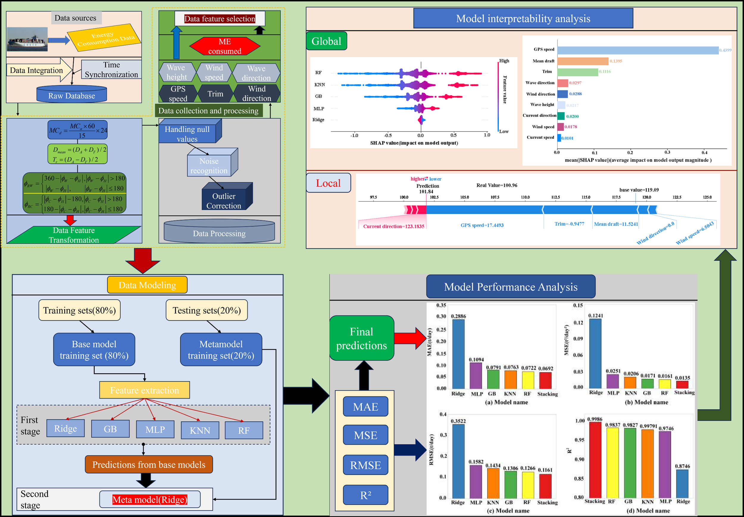
In this study, from data collection and processing, data modeling, performance analysis of the model to the interpretability analysis of the model, the accurate prediction of ship energy consumption and interpretability is gradually realized, and the specific technical roadmap is shown in Figure 1.
Figure 1
Technical roadmap.
Step 1: Data collection and processing. Through the collection of multi-source data such as main engine energy consumption, navigation status and maritime environment. Subsequently, frequency synchronization, data cleaning and feature processing are carried out to construct a unified dataset, which lays a solid data foundation for subsequent modeling.
Step 2: Data modeling. Data modeling is the core step in the technical route. First, the current mainstream ship energy modeling methods (10 different single models) are selected. Then, based on the residual correlation among the ten models, six groups of weakly correlated heterogeneous model combinations (A-F) were selected from 240 possible combinations as base models by setting a correlation coefficient threshold (<0.8). Finally, Ridge regression (Ridge) is selected as the meta-model of Stacking fusion model, which improves the prediction performance of the model through the fusion mode of two-layer prediction.
Step 3: Model performance analysis. The model performance analysis quantitatively measures the prediction performance of the model through four performance indicators: MAE, MSE, RMSE, and R², and verifies the performance advantages of the Stacking model compared with a single model in energy consumption prediction.
Step 4: Model interpretability analysis. The SHAP interpretability method is used to analyze the ship energy consumption fusion model at two levels, and to analyze the specific contributions of different base models and different input features to ship energy consumption.
2.2 Fusion model based on the stacking framework
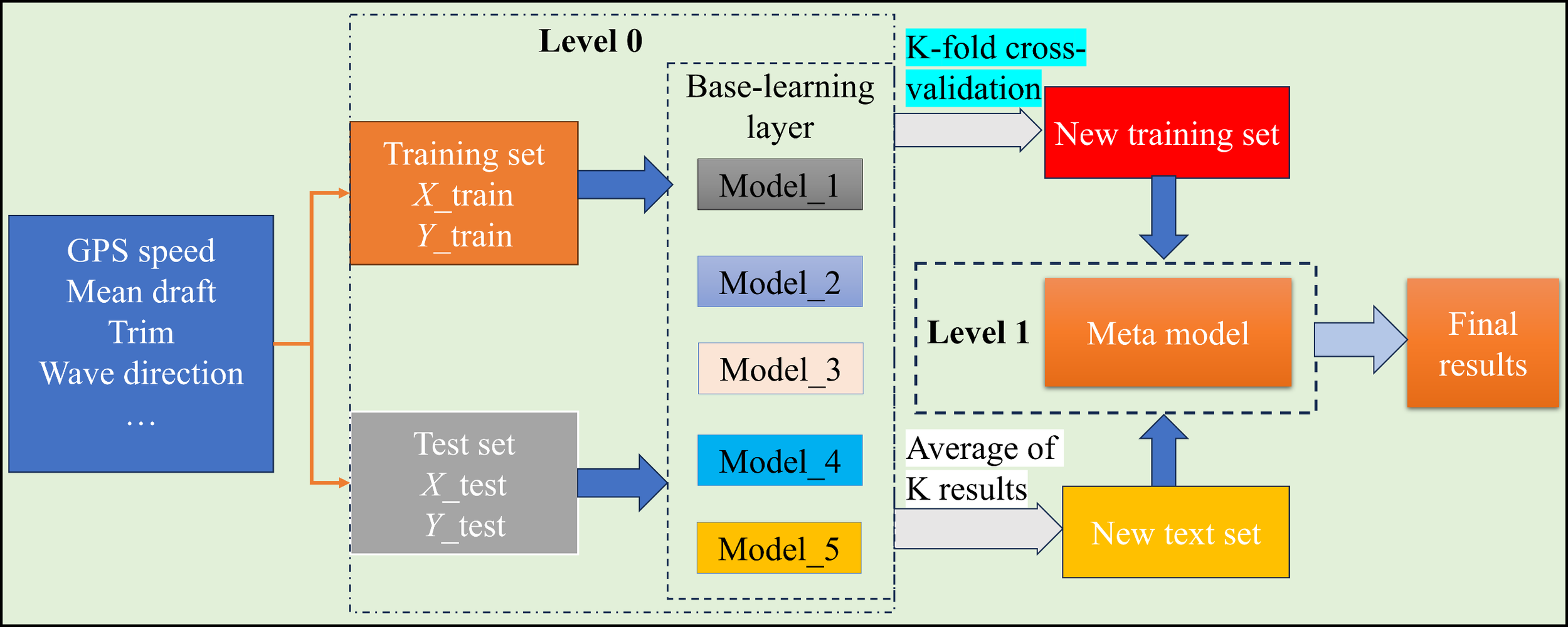
Stacking fusion model is a multilevel machine learning framework, which aims to improve the generalization ability and prediction accuracy of the model through the combination of multiple Base Learners and a Meta Learner. The core idea is to utilize the diversity of different Base Learners so that each of them learns different features of the data, and synthesize the outputs of each base model through the Meta Learner to obtain the final prediction results. The working principle and process of the Stacking fusion model specific to this study is shown in Figure 2.
Figure 2
The diagram of the stacking model framework.
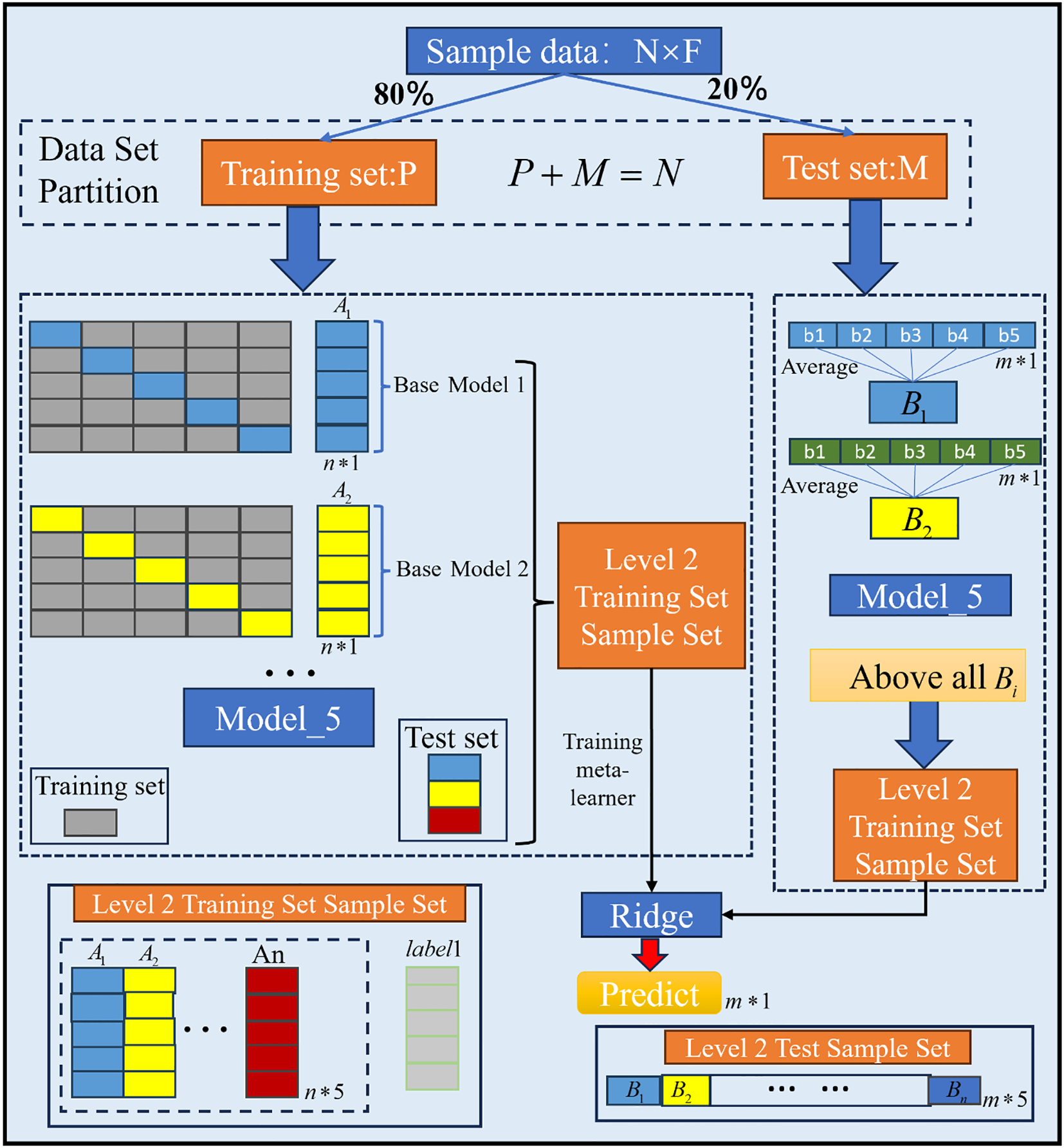
In the workflow of Stacking, firstly, the input data is divided into training set and test set, and the training set is further split by means of fold cross-validation to ensure that the base model is not overfitted, as shown in Figure 3. In each cross-validation, fold data is used for training and the remaining portion is used for validation, where each base model is trained on a different data division and predictions are generated. Subsequently, the predicted outputs of all base learners are stacked to form a new feature set that consists of the predicted values of each base model on the training data, while the true labels remain unchanged. This new feature set is used to train the meta-learner, whose role is to learn the relationships between the base models and generate the final predictions. In the testing phase, the test data is first passed through the trained base learner to generate multiple predictions, which are then averaged and connected to form a new test set, and then the trained meta-learner is used to predict the new test set, which ultimately generates more accurate predictions. The advantage of Stacking method is that it can combine different types of models, such as linear regression, decision tree, neural network, etc., so as to give full play to their respective advantages and avoid the limitations of single model.
Figure 3
K-fold cross-validation plot in Stacking. * indicates matrix multiplication in the context of the machine learning model structure. It represents the operation between matrices during the stacking ensemble process.
The Stacking fusion model in this study consists of a training process and a testing process. Training process.
1. The ship energy consumption data ( is the number of samples, is the number of features) is divided into a training set and a test set (where ).
2. Using fold cross validation for each base model, the data are divided into mutually exclusive subsets, where subsets are used as the training set and 1 subset is used as the validation set. Each base learner is trained on these training sets and predicted on the corresponding validation sets, thus obtaining the prediction results of each model on the validation sets. Subsequently, these predictions are stacked by rows to obtain the new feature vectors of the training set .
3. Splice the new feature vector to get the feature matrix ( is the number of training samples, is the number of base learners).
4. Train the meta-learner with the new spliced feature matrix and labels to get the final model. Testing process.
1. Calculate the prediction results of the samples in the test set using the previously trained model to form a 1-dimensional line prediction vector .
2. Average the prediction results of each model, and then stack the outputs of these models in columns to form a new data in dimensions ( represents the number of test samples, represents the number of base learners), and the next layer of models (meta-learners) will be further trained based on them.
3) Calculate the prediction results of using the Stacking fusion learning model obtained in the training phase, where is the test result of the stacking fusion learning model.
2.3 SHAP interpretability
The SHAP (SHapley Additive exPlanations) algorithm is a powerful and widely used tool for interpreting the outputs of complex models, helping to understand how the model arrives at its predictions, and improving the transparency of the model. SHAP originates from cooperative game theory. Its core idea is to consider all possible combinations of features, calculate the contribution of each feature to the predicted value in different combinations, then weight the average of these marginal contributions, and finally obtain the SHAP value of the feature. In ship energy consumption prediction, SHAP algorithm can be used to explain the contribution of different factors, such as wind speed and GPS speed, to make the prediction results more interpretable. Shapley value is defined as follows:
Let the feature set , the Shapley value of feature calculate its marginal contribution expectation before and after adding :
where, is the set of all features, is any subset of that does not contain the feature , is the predicted value of the model that only contains the subset of, is the predicted value of the model after adding the feature to the subset , denotes the size of the subset , and is the factorial of the total number of features to denote the full arrangement of features.
The predicted values of the model are decomposed by SHAP into the baseline values and feature contribution values, and the formula is as follows.
where, is the predicted value of the model, is the baseline value, is the SHAP value of the th feature, is the expectation of the predicted value of all possible samples.
2.4 Evaluation criteria
In order to quantitatively measure the difference in prediction performance between the Stacking fusion model and the base model, four types of metrics, Mean Absolute Error (MAE), Mean Square Error (MSE), Root Mean Square Error (RMSE), and Coefficient of Determination (R²), are used in this study.
1. Mean Absolute Error (MAE).
MAE is defined as the arithmetic mean of the absolute deviation between the predicted value and the real value, and its mathematical expression is:
Where is the real energy consumption value of the first sample, is the predicted value of the model, and is the total number of samples. MAE directly reflects the average absolute deviation between the predicted value of the model and the real energy consumption value, and the unit is consistent with the energy consumption scale.
2. Mean Squared Error (MSE).
Mean Squared Error (MSE) is the average of the squared error between the predicted value and the true value of the sample, which is defined as:
The unit of MSE is the square of the energy consumption measure, and the smaller its value is, the closer the model prediction is to the real value; the larger the value is, the larger the prediction deviation is. The significance of the symbols in the formula is the same as the mean absolute error (MAE).
3. Root Mean Squared Error (RMSE).
RMSE is the square root of MSE, and its expression is:
The unit scale of RMSE is consistent with the original data, reflecting the degree of deviation of the predicted value from the true value, the value range is [0, +∞), the smaller the value indicates that the model prediction accuracy is higher.
4. Coefficient of Determination ().
The degree of fit is defined as the proportion of the total variance explained by the model to the total variance of the data, and its calculation formula is:
where is the mean value of the true energy consumption. It is the core indicator of the model’s goodness of fit, and its value ranges from , and the closer the value is to 1, the stronger the model’s ability to explain the variance of the data.
3 Case study
3.1 Data sources
In order to evaluate the effectiveness of the proposed method, a representative 10,000-unit class container ship is selected as the object of this study, and the specific information of the container ship, see Table 1.
Table 1
| Parameter | Numerical value | Parameter | Numerical value |
|---|---|---|---|
| Length(m) | 349 | TEU | 10060 |
| Width(m) | 46 | Gross tonnage(t) | 114394 |
| Design speed(kn) | 24.8 | Year | 2007 |
| Maximum draught(m) | 14.5 |
Container ship information.
A total of 24,386 operational data were collected for the study object from September 14, 2017 to September 25, 2018, which were used to carry out the modeling analysis of the ship’s main engine energy consumption. Compared with the auxiliary engine and boiler system, which have stable energy consumption characteristics, the dynamic characteristics of main engine energy consumption have more significant research value for fuel efficiency optimization and operation cost control.
3.2 Data processing
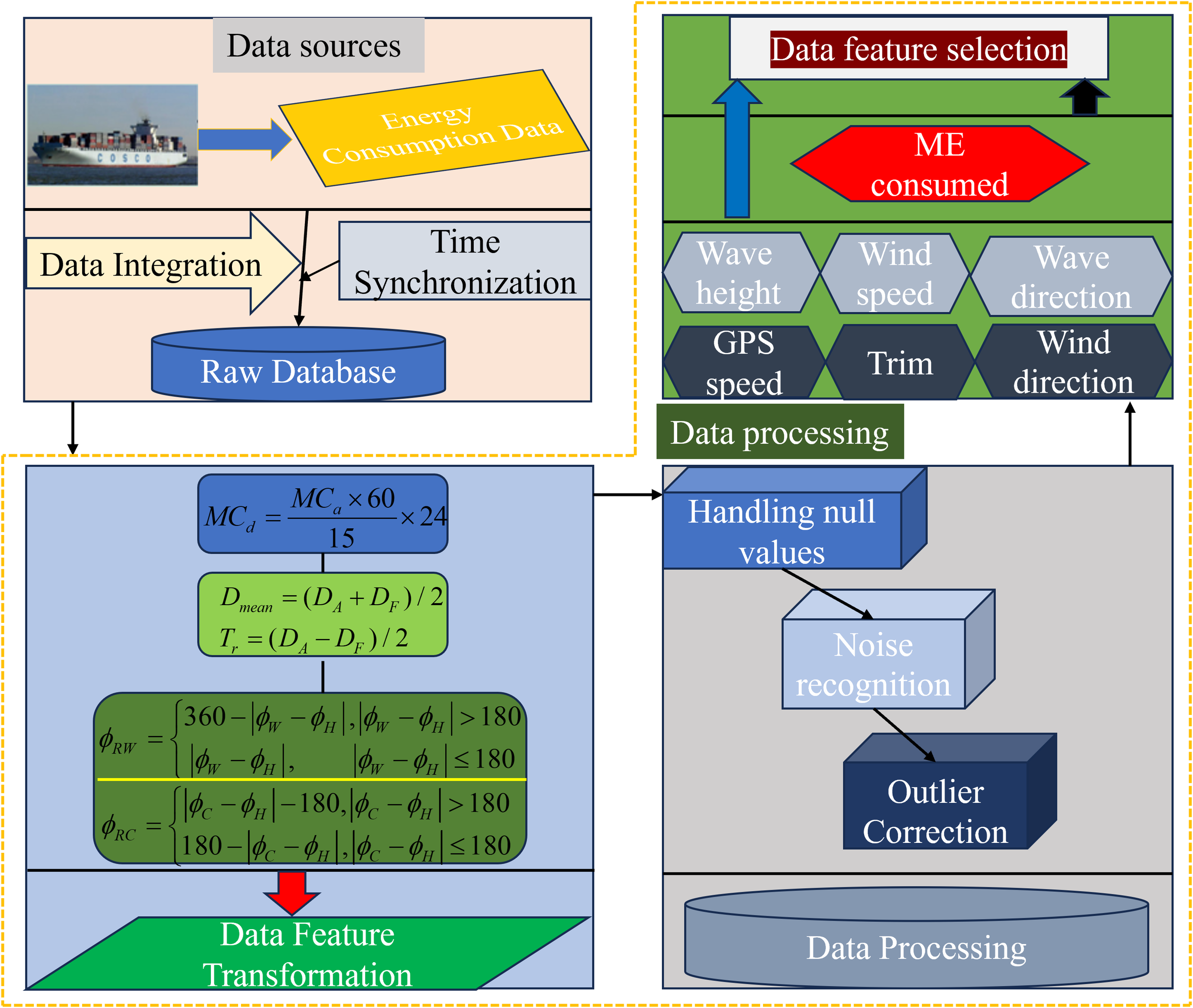
To establish a high-precision ship energy consumption prediction model, the construction of a high-quality ship energy consumption dataset is an important prerequisite. Therefore, a universal ship energy consumption data processing method is designed, from the initial data integration and time synchronization, to the feature conversion of energy consumption data, as well as the processing of null, noise and anomaly data, to the final feature selection, and finally obtain the high-quality ship energy consumption dataset, as shown in Figure 4, the formula in Figure 4 refers to Table 2.
Figure 4
Ship energy consumption data processing flow.
Table 2
| Data feature conversion | Characteristic conversion formula | Formula conformity interpretation | |
|---|---|---|---|
| Characteristic conversion of main engine energy consumption | is the daily energy consumption, is the main engine energy consumption of the container ship in every 15 minutes | ||
| Bow and Stern Draft Characteristic Conversion | Mean draft | is the bow draft, is the stern draft | |
| Trim | |||
| Conversion of wind, wave and current relative direction characteristics | Wind, Wave | is the true direction of wind, is the sailing direction, i.e., the direction of bow to | |
| Currents | is the true direction of current | ||
Data feature conversion.
3.2.1 Data integration and time synchronization
First, data from different sources, including host fuel consumption, navigation parameters, and environmental conditions, are collected at different frequencies, resulting in different amounts of feature data that cannot be directly used for modeling. Therefore, a key step is to ensure that all data streams are temporally consistent. Given that the host’s energy consumption data is recorded at 15-minute intervals, all other relevant feature data is synchronized with this frequency to construct a unified dataset, as shown Table 3. The dataset adopts a standardized 15-minute collection frequency, which completely records the core parameters including main engine energy consumption, rotational speed, and ground speed, and at the same time covers multi-dimensional navigational environment parameters such as bow/transom draught, marine meteorology (wind direction/wind speed/current speed), and sea state (wave height/direction), so as to ensure the consistency of the data and the continuity of the time series.
Table 3
| Feathers | Unite | Input/output | 2017.9.14 11:45 | … | 2017.9.14 13:00 | 2017.9.14 13:15 | 2017.9.14 13:30 | … |
|---|---|---|---|---|---|---|---|---|
| Main engine energy consumption | t/15min | Output | 0.3837 | … | 0.3284 | 0.3120 | 0.3123 | … |
| Main engine speed | rmp | Input | 42.3084 | … | 42.5711 | 42.5593 | 42.5811 | … |
| GPS speed | kn | Input | 11.0420 | … | 11.9879 | 11.9701 | 11.9760 | … |
| Mean draft | m | Input | 9.69292 | … | 9.59618 | 9.59026 | 9.59124 | … |
| Trim | m | Input | 0.766985 | … | 0.766 | 0.771923 | 0.772913 | … |
| Wind speed | m/s | Input | 0.697667 | … | 2.32159 | 1.79544 | 1.61577 | … |
| wind direction | ° | Input | 199.2 | … | 310.5 | 310.5 | 310.5 | … |
| wave height | m | Input | 0.8000 | … | 1.1000 | 1.1000 | 1.1000 | … |
| wave direction | ° | Input | 228.5000 | … | 242.8000 | 242.8000 | 242.8000 | … |
| Current speed | kn | Input | 0.2 | … | 0.1 | 0.1 | 0.1 | … |
| current direction | ° | Input | 129 | … | 101.7 | 101.7 | 101.7 | … |
Container ship energy consumption raw data sample.
To further illustrate the distribution characteristics of the collected dataset, Figure 5 presents the boxplot visualization of the main input variables. The figure shows that GPS speed, mean draft, and trim have relatively concentrated distributions, while environmental factors such as wind and wave direction exhibit wider ranges and larger variability, reflecting the complex and dynamic nature of marine conditions. The range of main engine (ME) consumption also demonstrates clear fluctuations, consistent with the variations in vessel speed and sea states. Overall, this visualization helps to provide an intuitive understanding of the dataset and supports the subsequent model analysis and validation.
Figure 5
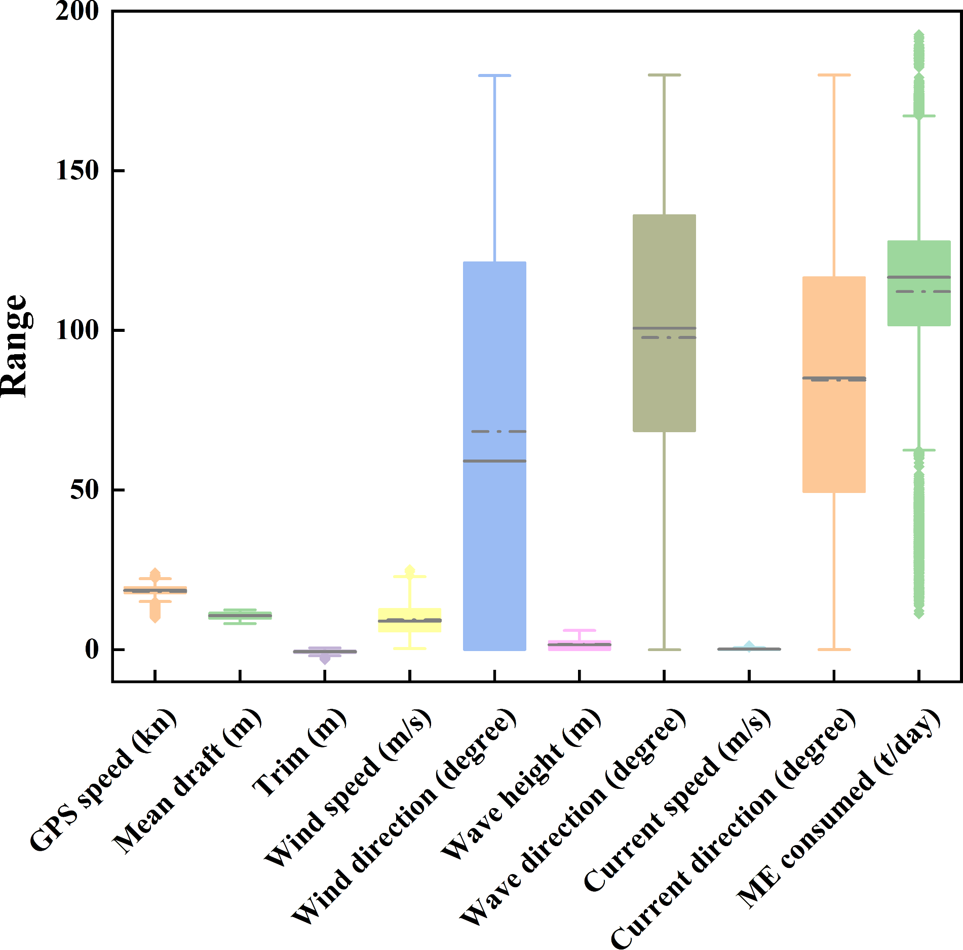
Boxplot of data feature distributions.
3.2.2 Data characterization
In order to construct more meaningful feature variables for the ship energy consumption prediction model of this study, the features of main engine energy consumption, bow and stern drafts, as well as meteorological information (wind direction) and sea state information (wave direction and current direction) are converted by combining the data features in Table 2.
3.2.3 Data processing
The data preprocessing procedure in this study mainly follows the framework proposed by (Hu et al., 2022), which has been widely applied in ship energy consumption and trim optimization research. To ensure data quality and consistency, all sensor data with different sampling frequencies were synchronized to a 15-minute interval. Missing values in key parameters such as main engine energy consumption and GPS speed were filled using a moving average interpolation.
Outliers were detected through a rate-of-change threshold and the interquartile range (IQR) method and were corrected or removed after cross-validation with ship operation logs. Noise caused by sensor drift or sea-state interference was filtered using a sliding window smoothing technique. To guarantee physical rationality, samples violating the basic relationship between ship speed and energy consumption were excluded.
Directional features such as wind and current directions were decomposed into sine and cosine components to maintain continuity. All numerical variables were normalized to [0,1] using the min–max method. Feature selection was carried out using a two-step process combining Pearson correlation and Variance Inflation Factor (VIF) analysis to remove weakly related or highly collinear variables (VIF< 5).
This workflow ensures statistical robustness and physical interpretability of the processed data. The general data alignment logic also refers to (Xiao et al., 2025), which provides a consistent approach for maritime multi-source data handling.
3.2.4 Data feature selection
To improve the accuracy and interpretability of ship energy consumption prediction models, it is necessary to screen out input features that have a significant impact on main engine energy consumption from numerous variables. The selection of input features was guided by both statistical measures and domain knowledge to enhance model performance and interpretability. A two-step feature screening methodology was employed. First, Pearson correlation analysis was conducted to identify variables exhibiting a strong linear relationship (|r| > 0.6) with ship energy consumption. Subsequently, to mitigate the issue of multicollinearity, the Variance Inflation Factor (VIF) was calculated, and features with a VIF value exceeding 5 were eliminated. This rigorous process ensured that the final feature set was not only statistically predictive but also physically meaningful and non-redundant, providing a robust foundation for model training.
Combining the theory of ship propulsion, domain knowledge and previous research experience, nine types of input features are preliminarily selected as the basis of data modeling, as shown in Table 4.
Table 4
| Sailing environment parameters | Input characteristics |
|---|---|
| Vessel operating parameters | GPS speed, Mean draft, Trim |
| Marine meteorological parameters | Wind speed, wind direction, wave height, wave direction |
| Ocean current information | Current speed, current direction |
Input Characteristics.
The output characteristic is daily main engine fuel consumption (ME consumed). The above features cover two categories: ship operating parameters and environmental factors. This set of selected features aims to capture the most important factors affecting ship energy consumption. For the specific feature selection method, please refer to the reference (Hu et al., 2022).
3.3 Data analysis
After the data processing Data processing, a total of 7493 valid records were retained. In order to analyze the effect of input variables on the main engine fuel consumption (ME consumed), this paper shows the relationship between the combination of five groups of variables and the energy consumption in a three-dimensional surface diagram, as shown in Figure 6.
Figure 6
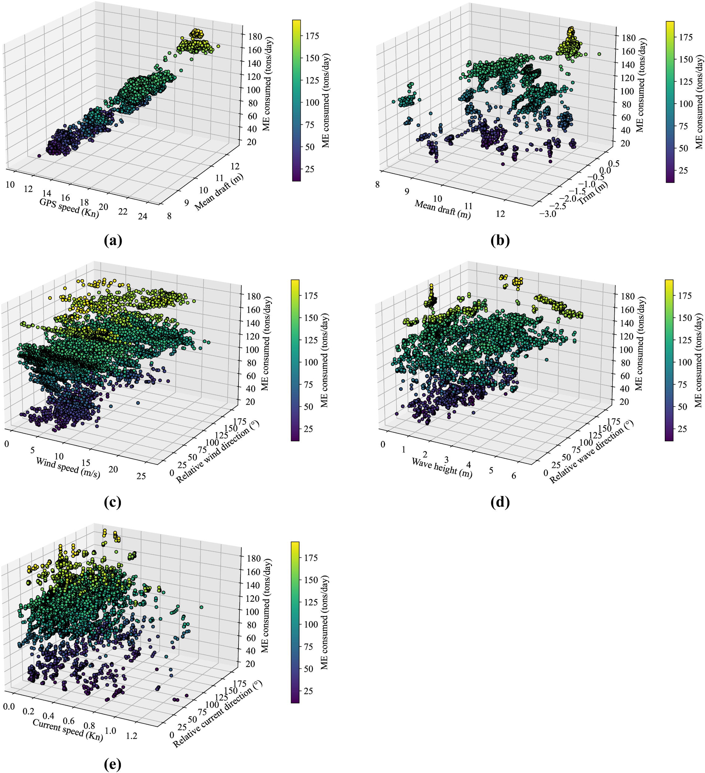
(a–e) Container ship characteristic data distribution.
Figure 6a shows the effect of GPS speed and mean draft on main engine energy consumption. The daily main engine energy consumption of the ship is mainly concentrated in 100–140 tons/day, and the speed is concentrated in the range of 17–20 knots. With the increase of speed, the energy consumption shows a steep upward trend, which is in line with the physical law of the speed-cubic relationship; under the same draft condition, the effect of speed on energy consumption is particularly significant, and the overall energy consumption level is higher under high draft condition (>11 m). Figure 6b shows the relationship between mean draft and trim on fuel consumption. At greater drafts (e.g., 11 m or more), when the trim is negative (bow trim), energy consumption increases significantly; whereas when the trim is close to zero or slightly positive (stern trim), energy consumption is relatively low under the same draft conditions. Figure 6c shows the effect of wind speed and relative wind direction on the fuel consumption of the main engine. When wind speeds exceed 15 m/s, the main unit’s energy consumption increases significantly. However, within the mainstream wind speed range of approximately 8 m/s, energy consumption remains relatively stable, indicating that wind direction has a limited impact on energy consumption under moderate to low wind speed conditions. Figure 6d shows the three-dimensional relationship between wave height and relative wave direction on energy consumption. When the wave height exceeds 2.0 m, the energy consumption shows a significant increasing trend. Most of the data are distributed in the range of 0-1.0 m. The energy consumption of the main engine corresponding to fluctuates less, which indicates that the energy consumption remains relatively stable in the middle and low wave conditions. Figure 6e reveals the effects of current speed and current direction on energy consumption. In the main interval where the current speed is less than 0.5 knots, the energy consumption distribution is relatively stable; however, when the current speed is more than 1.0 knots, the energy consumption shows a rapid increasing trend.
Overall, the changes of the ship’s own operating parameters (e.g., speed, draft, longitudinal inclination) have a decisive effect on the energy consumption, while the environmental factors such as wind, waves, and currents have a certain influence on the energy consumption under a specific combination of intensity and direction.
4 Results and discussion
All experiments in this study were conducted based on Python version 3.12 running on a 64-bit Windows 11 operating system, a 12th Gen Intel(R) Core (TM) i5-12500H 2.50 GHz CPU processor and 16.0 GB of RAM. The version of sklearn primarily used for modeling is 1.5.2, the version of Optuna is 4.1.0, and the version of SHAP is 0.46.0.
4.1 Stacking base model and meta-model selection
4.1.1 Selection of base model
In the fusion modeling framework, Stacking combines the predictions of multiple base models by combining the predictions of multiple base models and then using meta-models to predict the results of the base models again. However, the selection of base models needs to balance the accuracy and diversity of model predictions (Baraheni et al., 2024) in order to avoid overfitting and enhance the fusion effect. In this study, we introduce the residual correlation analysis method (Wang and Chi, 2024) to quantify ten mainstream machine learning models (Tufail et al., 2023): linear regression LR, ridge regression Ridge, decision tree DT, random forest RF, gradient boosting GB, support vector regression SVR, k-nearest neighbor KNN, multilayer perceptron MLP, XGBoost and Convolutional Neural Network CNN (Cira et al., 2023), whose results are shown in Figure 7.
Figure 7
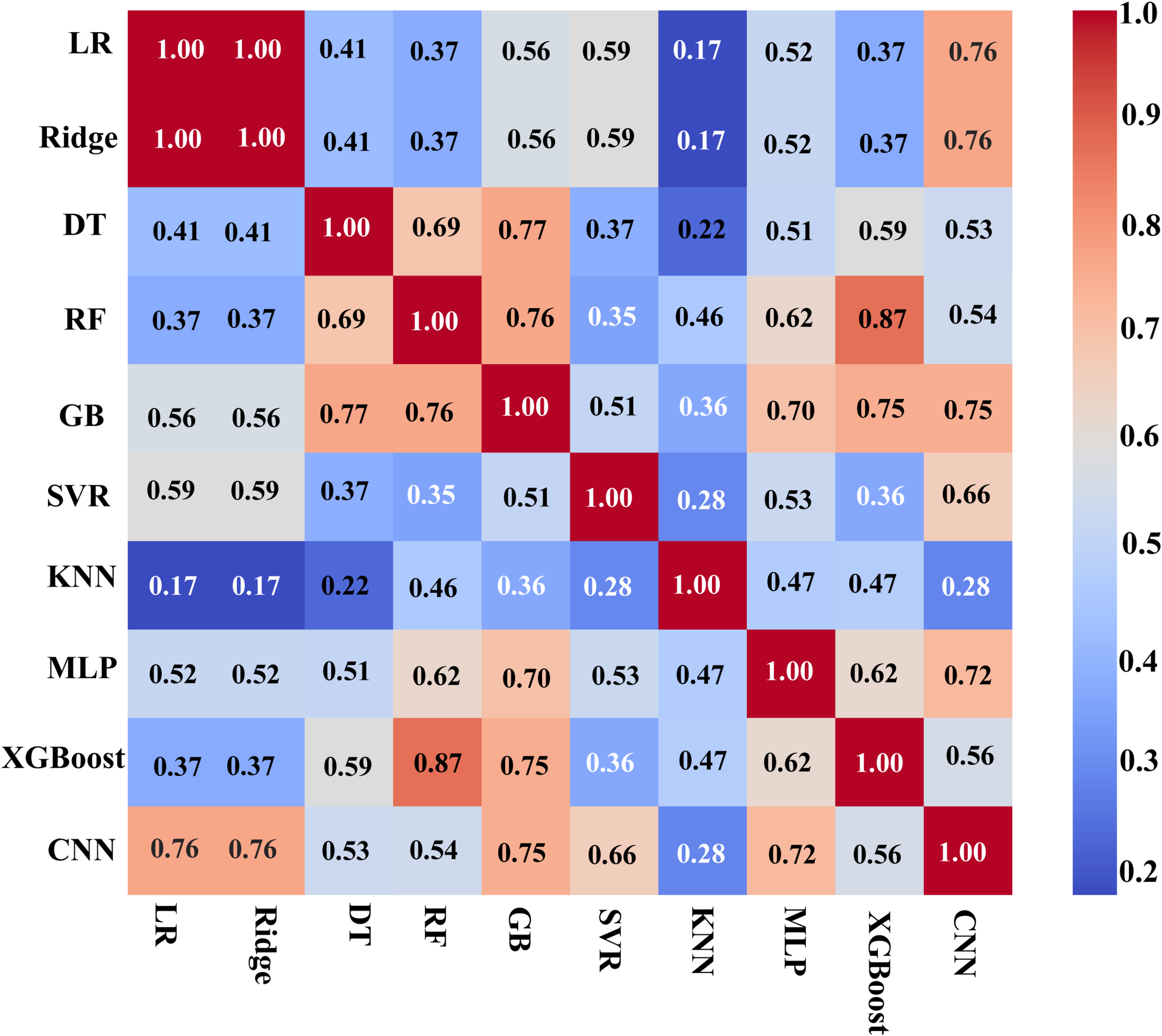
Residual correlation matrix of different models.
The residual correlation matrix reflects the degree of linear correlation between the prediction errors of different models. If the residuals of two models are highly correlated (e.g., the correlation coefficient of LR and Ridge is 1.00), it indicates that their error patterns are highly convergent, and it is difficult to improve the performance through fusion after combination; on the contrary, low-correlation models (e.g., the correlation coefficient of KNN and CNN is 0.28) may enhance the generalization ability and prediction accuracy of the fusion model due to the complementarity of errors.
By setting a correlation coefficient threshold (<0.8) (Kuncheva and Whitaker, 2003; Brown et al., 2005), six sets of weakly correlated heterogeneous model combinations (A-F) were screened out from 240 possible combinations, covering linear models, tree models, and neural networks, which to some extent solves the problem of the subjectivity of the selection of the base model in the traditional approach. Taking Combination B (Ridge, GB, MLP, KNN, RF) as an example, the residual correlation coefficients of the base models are between 0.17 (KNN and Ridge) and 0.76 (GB and RF), which contains both high-precision models (GB and RF) and achieves complementary errors by introducing the low-correlation KNN and MLP. Similarly, the combination F (LR, DT, SVR, KNN, XGBoost) covers multiple learning mechanisms while maintaining diversity by fusing linear models (LR), tree models (DT, XGBoost) and kernel methods (SVR). Through the above selection strategy, six representative combinations (A-F) are finally selected and their composition is shown in Table 5.
Table 5
| Portfolio | Model composition | Selection basis |
|---|---|---|
| A | LR DT SVR KNN CNN | Fusion of linear, tree, kernel methods and neural networks with residual correlation coefficients ranging from 0.17-0.74 |
| B | Ridge GB MLP KNN RF | Fusion of regularized linear, integrated learning and neural network models, Ridge controls overfitting, RF and GB provide integration benefits |
| C | DT GB SVR MLP XGB | Tree modeling and gradient boosting are at the core, with SVR and MLP enhancing nonlinear fitting capabilities |
| D | LR KNN GB XGB CNN | Mixed linear and nonlinear models, CNN extracts higher order features, XGB optimizes tree fusion |
| E | Ridge DT RF MLP CNN | Ridge regression constrains overfitting, RF and CNN enhance classification and feature learning respectively |
| F | LR DT SVR KNN XGB | Multi-mechanism fusion, XGB and SVR to handle structured and unstructured data respectively |
Stacking portfolio composition and selection basis.
In order to evaluate the performance of the six Stacking combinations, and then select the base model combination with the best prediction effect, this experiment uses MAE, MSE, RMSE, and R² as the performance evaluation indexes, and compares their prediction accuracies and stabilizations in six independent repetitive experiments. Taking the R² performance index as an example, through the bar chart of model performance comparison, the bar represents the combination, the dots above it indicate the results of a single experiment, and the error bars reflect the standard deviation of the mean of the six experiments, as shown in Figure 8. The experimental comparison results are clearly visible in the figure. Combination B shows the best performance, with an R² mean of 0.98632, higher than other combinations (such as combination F with R² = 0.98630). Therefore, Combination B (Ridge, GB, MLP, KNN, RF) was chosen as the base model in the Stacking fusion model of this study.
Figure 8
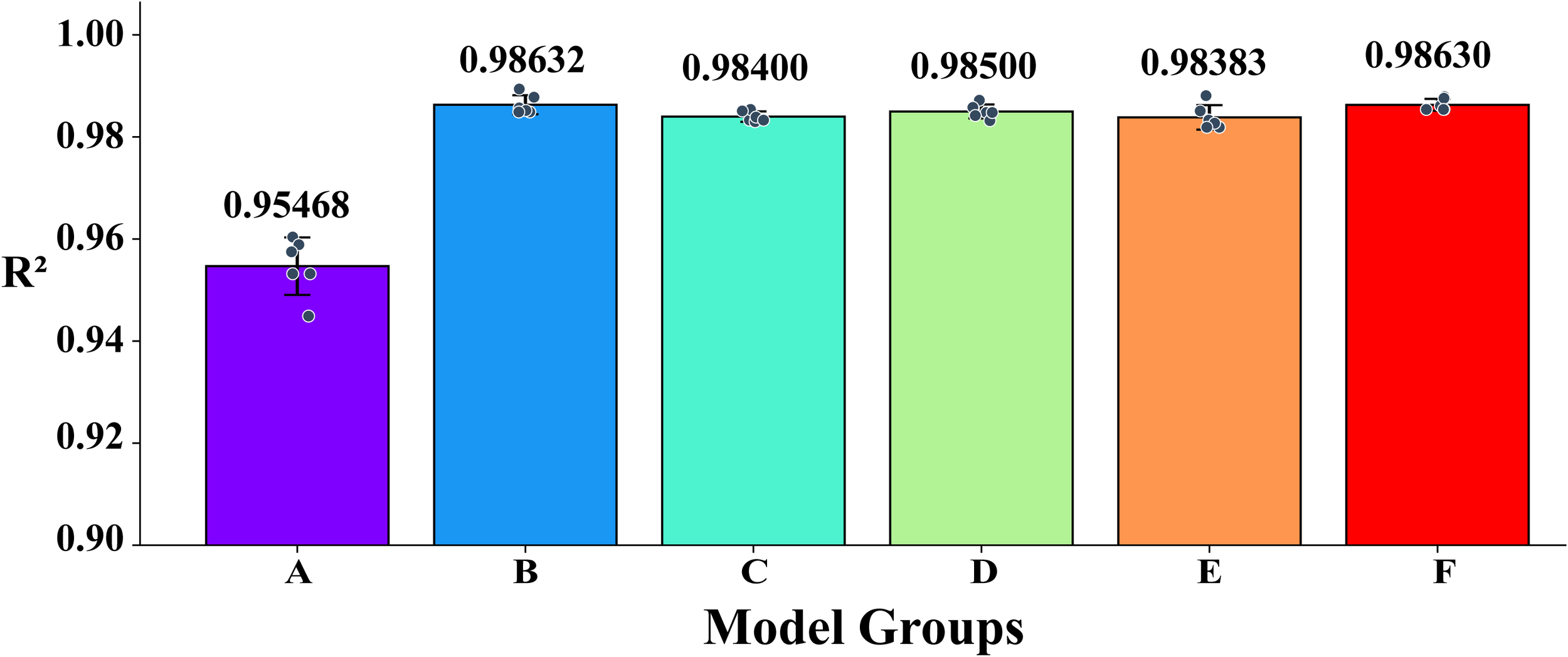
Comparison of R² performance of six combinations.
As shown in Figure 8, the R² performance of Combination A is slightly lower than that of the other model groups. This can be attributed to the fact that several models in Combination A (such as LR and DT) exhibit highly correlated residuals, resulting in redundant error patterns and reduced ensemble diversity. In contrast, Combination B was constructed under a residual correlation threshold (< 0.8), integrating heterogeneous and complementary models including Ridge, GB, MLP, KNN, and RF. This improved diversity leads to better error compensation among base learners and thus a higher overall R² (0.9863).
4.1.2 Selection of meta model
In Stacking fusion model, the metamodel should be as simple as possible and have certain stability and generalization ability (Wang et al., 2024d). Ridge regression integrates the base model prediction by linear weighting, and at the same time prevents overfitting effectively with the help of L2 regularization, which improves the stability of the model (Huang et al., 2024). Therefore, the Ridge regression was chosen as the meta-model in this study.
To verify the rationality of selecting Ridge as the meta-learner, additional comparative experiments were conducted using two nonlinear alternatives—Multilayer Perceptron (MLP) and Decision Tree (DT)—under identical base-model configurations and experimental settings. The results (as shown in Table 6) demonstrated that the Ridge-based stacking model consistently achieved the best overall performance, with lower MAE, MSE, and RMSE values and higher R² compared to the nonlinear counterparts. This indicates that the linear Ridge meta-learner offers more stable aggregation of the base-model predictions and effectively mitigates overfitting, thereby providing an optimal trade-off between model accuracy, robustness, and interpretability. Consequently, Ridge was selected as the final meta-model in the proposed stacking framework.
Table 6
| Model | meta_model | MAE | MSE | RMSE | R² |
|---|---|---|---|---|---|
| Stacking | Ridge | 0.0661 | 0.0114 | 0.107 | 0.9894 |
| MLP | 0.0676 | 0.0117 | 0.1084 | 0.9891 | |
| DT | 0.0878 | 0.0195 | 0.1398 | 0.9818 |
Comparative experiment of meta-model.
4.2 Comparison before and after hyperparameter optimization
Hyperparameter optimization is crucial for model prediction accuracy and generalization ability. To enhance the prediction accuracy and generalization capability of the Stacking fusion model, a structured hyperparameter optimization strategy was implemented. The optimization process was conducted using the Optuna framework, which employs a Bayesian optimization algorithm with the Tree-structured Parzen Estimator (TPE) as the sampling method. The objective was set to minimize the Root Mean Square Error (RMSE) on the validation set. This approach efficiently explores the hyperparameter space by leveraging past evaluation outcomes, thus accelerating convergence and mitigating the risk of settling into local optima, a common limitation of grid or random search techniques.
Considering the high cost of tuning, this study focuses on key hyperparameters. Based on the results of Stacking base model and meta-model selection chapter, the base model in the B combination (Ridge GB MLP KNN RF) is selected for hyperparameter optimization, and the parameter details of the related base model are shown in Table 7.
Table 7
| Models | Hyperparameter | Default value | Optimization range |
|---|---|---|---|
| Ridge | Ridge | 1.0 | 0.001 - 100 |
| KNN | n_neighbors | 5 n_neighbors | 1 - 20 |
| RF | n_estimators | 100 n_estimators | 50 - 300 |
| max_depth | max_depth | 5 - 50 | |
| n_estimators | n_estimators | 100 n_estimators | 50 - 300 |
| learning_rate | 0.1 | 0.01 - 1.0 | |
| max_depth | 1 - 10 | 1 - 10 | |
| MLP | hidden_layer_sizes | (100), | (50), (100), (150), |
| alpha | 0.0001 | 0.00001 - 0.01 | |
| learning_rate_init | 0.001 | 0.0001 - 0.01 |
Hyperparameter optimization information in the B-combination model.
This experiment optimizes the hyperparameters of the B combination experiment model using Optuna’s Bayesian optimization. By comparing the results before and after hyperparameter optimization, we verify its improvement in ship energy consumption prediction performance and visualize the four performance indicators before and after hyperparameter optimization, as shown in Figure 9.
Figure 9
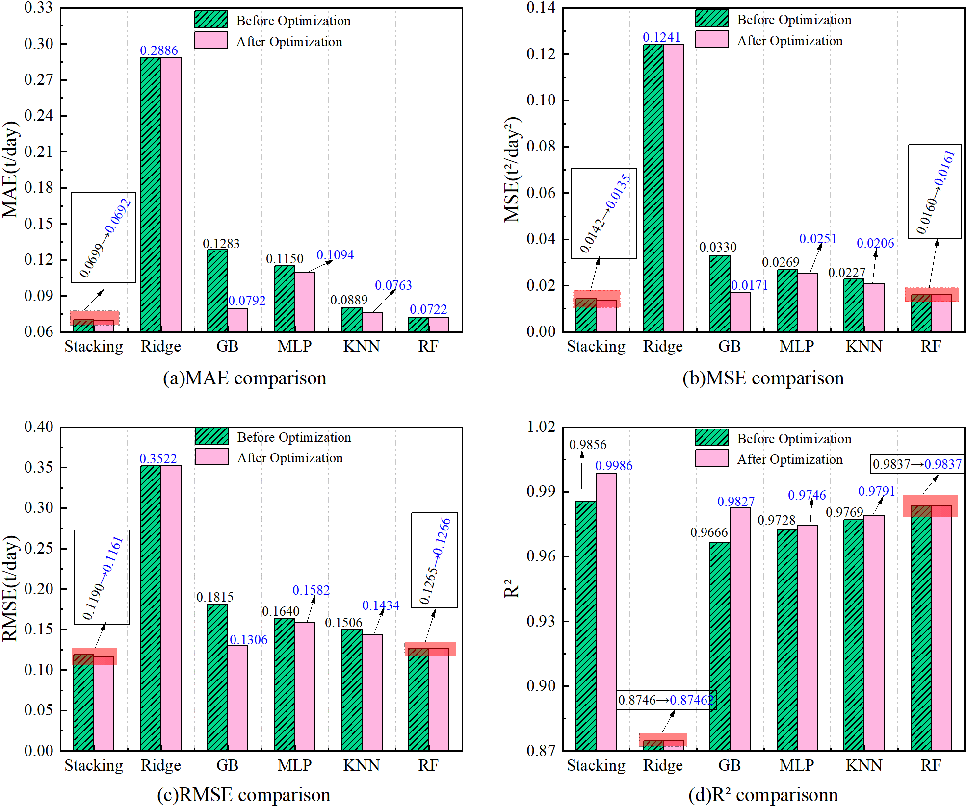
(a–d) Comparison of performance indicators before and after hyperparameter optimization.
As can be seen from the figure, after the hyperparameter optimization, the mean absolute error (MAE) of the fusion model is reduced from 0.0699 to 0.0692, a decrease of 1.00%; the mean square error (MSE) is optimized from 0.0142 to 0.0135, a decrease of 4.39%; the root mean square error (RMSE) is reduced from 0.1190 to 0.1161, a decrease of 2.44%; the coefficient of determination (R²) is improved from 0.9856 to 0.9986, an improvement of 1.32%. The above results show that after the hyper-parameter optimization method (Optuna), five base models (Ridge, GB, MLP, KNN, RF) and one fusion model, Stacking, have been improved to some extent in four performance metrics (MAE, MSE, RMES, R²).
4.3 Comparison of prediction performance results of different models
In order to verify the effectiveness of the established Stacking fusion model, the prediction performance of different models was compared and analyzed, as shown Figure 10. All the performance results are the average values of six experiments.
Figure 10
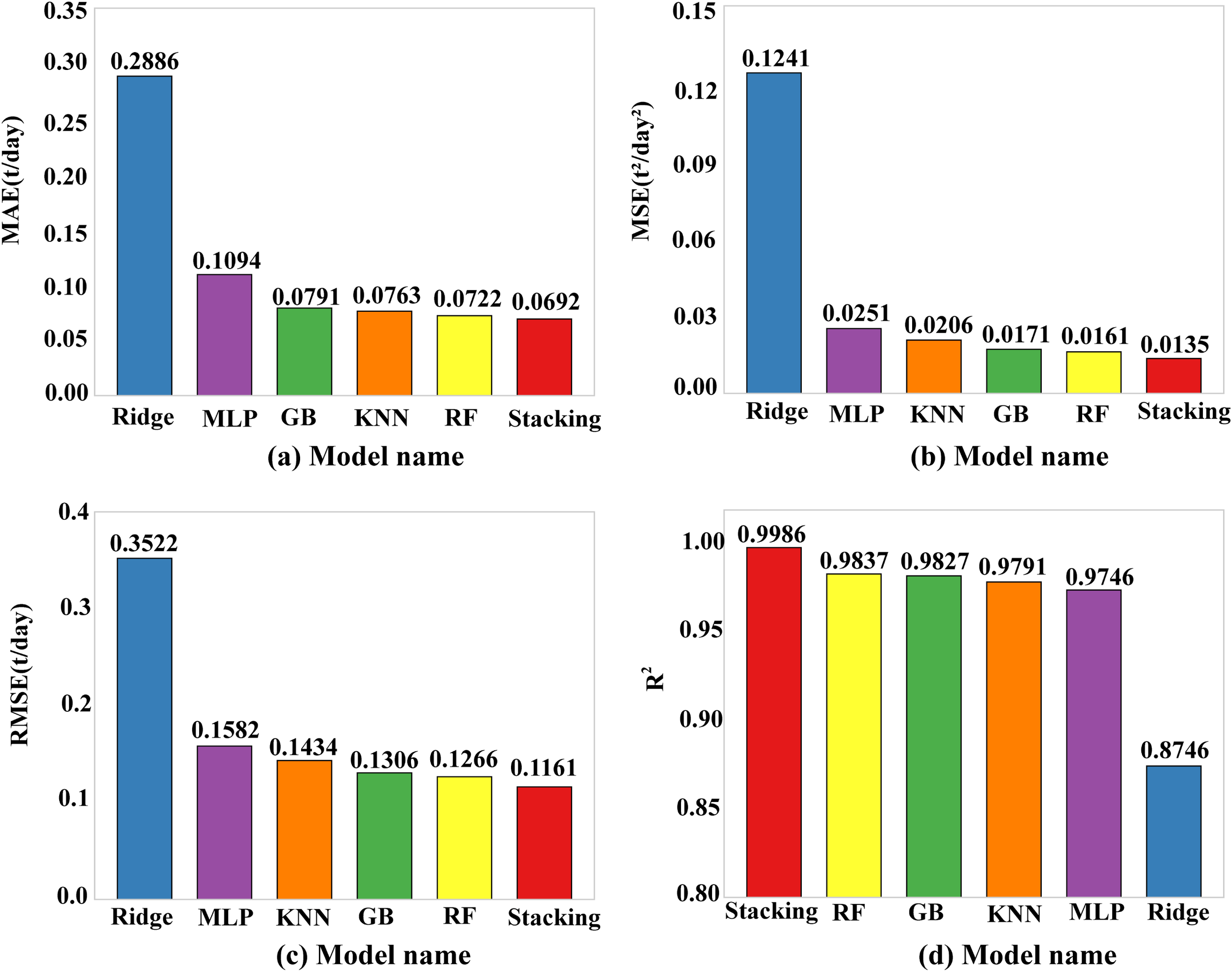
(a–d) Comparison of prediction performance results of different models.
From Figure 10, Stacking reduces 75.9%, 12.6%, 36.7%, 9.3%, and 4.1% at the MAE level compared to Ridge, GB, MLP, KNN, and RF, respectively. At the MSE level compared to Ridge, GB, MLP, KNN, and RF are 89.1%, 21.1%, 46.2%, 34.5%, and 16.1% lower, respectively. At the RMSE level it is 67.0%, 11.1%, 26.6%, 19.0%, and 8.3% lower compared to Ridge, GB, MLP, KNN, and RF, respectively. At the R² level it improves 14.2%, 1.6%, 2.5%, 2.0%, and 1.5% compared to Ridge, GB, MLP, KNN, and RF, respectively.
In light of the model comparison results presented in Figure 10 above, the corresponding data are summarized in Table 8.
Table 8
| Model | MAE | MSE | RMSE | R² |
|---|---|---|---|---|
| Stacking | 0.0692 | 0.0135 | 0.1161 | 0.9986 |
| Ridge | 0.2886 | 0.1241 | 0.3522 | 0.8746 |
| GB | 0.0791 | 0.0171 | 0.1306 | 0.9837 |
| MLP | 0.1094 | 0.0251 | 0.1582 | 0.9746 |
| KNN | 0.0763 | 0.0206 | 0.1434 | 0.9791 |
| RF | 0.0722 | 0.0161 | 0.1266 | 0.9837 |
Performance comparison of stacking vs. base models.
Based on the analysis of the above experimental data, Stacking further improves the accuracy of ship energy consumption prediction compared to the traditional single prediction model at the level of four performance indicators. Therefore, the Stacking fusion model constructed in this study has a certain degree of effectiveness.
4.4 SHAP interpretable model analysis
In Section 4.3, the predictive performance of the model was quantitatively evaluated using four performance metrics: MAE, MSE, RMSE, and R². This validated the advantages of the Stacking model in energy consumption prediction. However, it remains unclear how the Stacking model obtains its predictive results and how different input features influence the final output of the ensemble model. Therefore, the SHAP interpretability method is utilized to analyze the interpretability of the Stacking model at. In the following, a two-layer interpretability analysis will be performed globally and locally.
4.4.1 Global interpretability
Global interpretability refers to the explanation of the behavior and decision logic of the whole model, which provides a macro view to help understand how the model works as a whole.
4.4.1.1 Interpretability analysis of the contribution of the base model
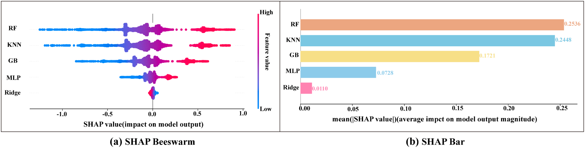
In this study, the SHAP values were used to comprehensively analyze the contribution of the base models to ship energy consumption. Through two visualization methods, SHAP Beeswarm plots and SHAP Bar plots, the contributions of each base model and their impact on the prediction results were revealed, as shown in Figure 11.
Figure 11
(a, b) Base model contribution value.
As can be seen from Figure 11a, the SHAP Beeswarm plot shows the distribution of SHAP values predicted by each base model for ship energy consumption. The horizontal axis indicates the magnitude of SHAP values, and the color reflects the high or low prediction value of the base model (red high and blue low). It can be clearly seen from the figure that the distribution of SHAP values for different base models shows significant differences. The SHAP values of the Random Forest (RF) model are widely distributed with large positive and negative fluctuations, indicating that it has an important role in determining the predicted value of ship energy consumption, while the distribution of the Ridge regression (Ridge) model is concentrated, with a smaller contribution and a more stable influence. Figure 11b. The RF model has the highest absolute average SHAP value (0.2536) and the strongest influence; KNN (about 0.2448) is the second highest; the GB model (0.1721) also plays an important role; MLP (0.0728) has relatively small influence; the Ridge model has the lowest average SHAP value (0.0110), the weakest contribution, may only provide stability or auxiliary support.
4.4.1.2 Interpretability analysis of input feature contributions
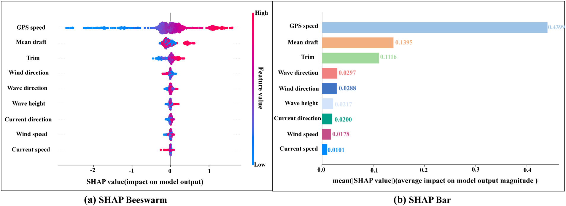
In the experiment to study the contribution of input features to ship energy consumption, two visualization effect plots, SHAP Beeswarm plot and SHAP Bar plot, are also used. These input features cover the ship’s own operating parameters as well as environmental factors, and the SHAP analysis and visualization effects are shown to reveal the role of each feature in the model and its contribution to the prediction of ship’s energy consumption, as shown in Figure 12.
Figure 12
(a, b) Input feature contribution value.
As can be seen from Figure 12a, the SHAP Beeswarm plot shows the distribution of the influence of the input features on the prediction of ship energy consumption. The horizontal axis indicates the size of the SHAP value and the color represents the feature taking high or low values (red high and blue low). It can be seen that GPS speed has the greatest influence on the model output, and the distribution of SHAP values shows obvious positive and negative poles, with high-speed corresponding to larger positive SHAP values and low speed corresponding to negative values, indicating that it has a key role in energy consumption prediction under different sailing conditions. Mean draft and Trim also show strong effects, with high values corresponding to positive SHAP values, which increase energy consumption, and low values corresponding to negative values, which help to reduce energy consumption. In contrast, the distribution of SHAP values for environmental factors such as wind direction, wave height, and flow direction is more scattered, and the overall values are small, contributing less and having a more stable effect.
Figure 12b shows the SHAP bar plot, which further quantifies the importance of the input features. GPS speed has the highest average SHAP value (0.4399), with the strongest influence; draft depth and trim come next, with average values of 0.1395 and 0.1116, respectively; and the rest of the environmental features, such as wave direction (0.0297) and wind direction (0.0288) have limited influences, with average SHAP values generally lower than 0.03. Overall, the distribution of environmental factors, such as wave height and current direction, is more dispersed, with overall values of less than 0.03, and their influences are more stable. On the whole, the ship’s own operating conditions contribute significantly to the energy consumption prediction, while the environmental factors play a relatively minor role.
The SHAP results indicate that sailing speed is by far the most dominant factor influencing ship energy consumption. This is physically consistent with the cubic relationship between propulsion power and vessel speed: as speed increases, the required engine power and thus fuel consumption rise exponentially. This also explains why the modern shipping industry increasingly advocates “slow steaming,” which effectively reduces fuel consumption and greenhouse gas emissions by operating at moderate speeds.
In addition, the longitudinal trim also exhibits a significant impact. A negative trim (bow-down condition) increases hull resistance and propeller load, thereby elevating the overall energy consumption, whereas maintaining near-neutral or slightly stern trim can improve hydrodynamic efficiency. These results not only validate the reliability of the SHAP-based interpretation but also provide practical guidance for operational optimization and energy-efficient navigation management.
4.4.2 Local interpretability
Local interpretability refers to the explanation of the prediction results of a specific sample in the ship energy consumption model, and focuses on the decision-making process of the model on a specific sample. Global interpretability provides a macroscopic understanding of the overall performance of the model, while local interpretability provides a refined explanation of individual decisions.
Two samples are randomly selected as examples of local interpretability, and force diagrams are used to visualize the contribution of each input feature to the predicted value of ship energy consumption, thus making the predicted value of the black-box model more transparent and interpretable. For example, Figure 13 In Sample 1, the actual value of SHAP is 126.7600, the predicted value is 128.4861, and the baseline value is 119.0899, with an absolute value of error of 1.7261. The GPS speed (20.4179) is the most dominant positive influencing factor (in red) in this sample, which dramatically improves the predicted value, due to the sample’s speed being higher than the average sailing speed in the dataset (18.2598 Kn). In addition, wave height, mean draft, wind speed, and wave direction all contributed positively, increasing ship energy consumption; trim and current direction contributed negatively, reducing ship energy consumption values.
Figure 13
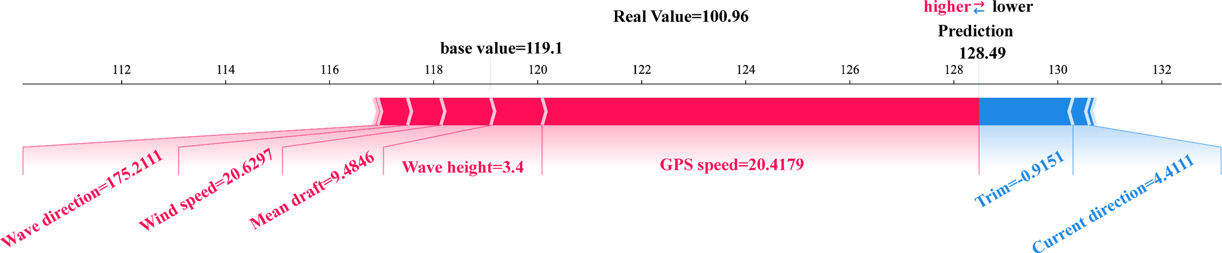
SHAP force plot (sample 1).
Figure 14 shows that the actual value of SHAP in Sample 2 is 100.9620, the predicted value is 101.8414, and the baseline value is 119.0892, with an absolute value of error of 0.8794. The main factor influencing the predicted value of the samples is the GPS speed (17.4493), which reduces the predicted value considerably due to the fact that the ship’s speed is lower than the average speed in the dataset (18.2598 Kn). This is due to the lower speed of the ship than the average speed in the dataset (18.2598 Kn), followed by trim (-0.9477) and mean draft (11.5241) which also reduce the predicted values.
Figure 14
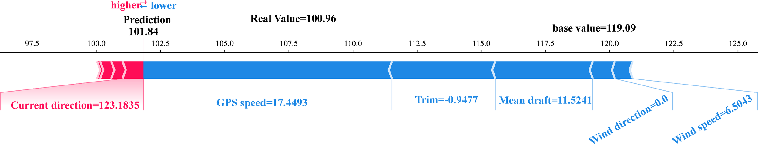
SHAP force plot (sample 2).
In order to present more clearly the contribution of different features to the prediction of energy consumption of the ship, all the input feature SHAP values for both samples are presented in the table, such as Table 9. A positive SHAP value indicates a positive effect and a negative one a negative effect. In Sample 1, the GPS speed of 20.4179 has a SHAP value of 8.4009, which is the largest positively influenced feature; the wind direction (84.4) and current direction (4.4111) contribute -0.1146 and -0.3203, respectively, which are negatively influenced. The total SHAP value of the nine features is 9.3968, and the baseline value is 119.0899, which results in a predicted value of 128.4861. The total SHAP value of the 9 features is -17.2479, and the baseline value of 119.0892 gives a predicted value of 101.8414. The predicted value is 101.8414.
Table 9
| Sample 1 | Sample 2 | ||
|---|---|---|---|
| Feature values | SHAP values | Feature values | SHAP values |
| GPS speed=20.4179 | 8.4009 | GPS speed=17.4493 | -9.6778 |
| Mean draft=9.4846 | 0.9589 | Mean draft=11.5241 | -3.7973 |
| Trim=-0.9151 | -1.8046 | Trim=-0.9477 | -4.0276 |
| Wind speed=20.6297 | 0.6408 | Wind speed=6.5043 | -0.6910 |
| Wind direction=84.4000 | -0.1146 | Wind direction=0.0000 | -0.8641 |
| Wave height=3.4000 | 0.9872 | Wave height=0.0000 | 0.4409 |
| Wave direction=175.2111 | 0.5737 | Wave direction=56.8165 | 0.4324 |
| Current speed=0.2000 | 0.0748 | Current speed=0.0000 | 0.1192 |
| Current direction=4.4111 | -0.3203 | Current direction=123.1835 | 0.8174 |
SHAP values of two samples.
In addition to interpreting the SHAP results, it is also important to verify the robustness of feature importance to ensure reliable interpretation. Hu et al. (2021) in the previous study, environmental features such as wind, wave, and current were examined through comparative modeling under different input combinations. The findings indicated that excluding these environmental variables led to only a slight reduction in prediction accuracy and did not alter the dominant influence of speed and trim on fuel consumption. This consistency supports the reliability and physical validity of the SHAP-derived feature importance obtained in the present work. Nevertheless, we recognize the necessity of a more systematic assessment, and future research will include feature-dropping and substitution sensitivity tests to quantitatively evaluate the model’s stability and robustness under varying feature sets.
5 Conclusion
In order to improve the accuracy and model interpretability of ship energy consumption prediction, this study proposes a ship energy consumption prediction framework based on the Stacking fusion model and SHAP interpretability analysis, which improves the overall prediction performance of the model by combining the advantages of multiple single models, and at the same time adopts the SHAP interpretability analysis to further improve the transparency of the prediction results of the ship energy consumption model, and to increase its credibility. A large container ship is taken as the research object to verify the effectiveness of the proposed model, and the experimental results and conclusions obtained are as follows:
-
In terms of model prediction accuracy, the energy consumption prediction model based on Stacking fusion constructed in this paper effectively improves the model performance by introducing heterogeneous base models such as Ridge, GB, MLP, KNN and RF, and integrating modeling with Ridge as the meta-learners, combined with Optuna for hyper-parameter optimization. The experimental results show that the optimized model achieves 0.0692, 0.0135, 0.1161, and 0.9986 in the four metrics of MAE, MSE, RMSE, and R², respectively, which are 4.1%, 16.1%, 8.3%, and 1.5% higher than the optimal single model RF. Compared with the base models such as Ridge, GB, and MLP, the Stacking model achieves the maximum improvement of 75.9%, 89.1%, 67.0%, and 14.2% in the four metrics, respectively. The above results show that Stacking overcomes the problems of overfitting and bias accumulation of a single model by complementing multiple models, and significantly improves the accuracy of energy consumption prediction while ensuring stability.
-
In terms of model prediction interpretability, in order to enhance the transparency and credibility of the model, this paper adopts the SHAP method to analyze the global and local two-layer interpretability of the Stacking fusion model. At the base model level, the average SHAP values of RF, KNN, and GB are 0.2536, 0.2448, and 0.1721, respectively, with a total contribution of more than 67%, which is the core support of the fusion model; while the contributions of MLP (0.0728) and Ridge (0.0110) are relatively low. At the level of input characteristics, GPS speed (0.4399), mean draft (0.1395) and longitudinal inclination (0.1116) are the top three main influences, accounting for 69.1%, which is in line with ship propulsion theory. In terms of local interpretation, SHAP seeks to clearly reveal the positive and negative influence paths of individual features on the single-sample predicted values, realizing the visual deconstruction of the black-box model. The analysis provides quantitative basis and transparent support for model credibility validation and energy efficiency optimization in shipping management.
The method proposed in this paper not only achieves better improvement in prediction accuracy, but also enhances the interpretability of the model, which provides a theoretical basis and practical path for constructing a high-performance and high-transparency ship energy consumption prediction system.
Nevertheless, several limitations should be acknowledged. The current model was developed and validated using operational data from a single post-Panamax container vessel within one year, which may introduce vessel-specific or temporal bias and thus limit its generalization. Although cross-validation and repeated experiments were conducted to mitigate possible overfitting, the model may still capture route- or ship-dependent characteristics. Furthermore, potential data quality issues—such as sensor noise, missing records, or inconsistencies in environmental parameters—may affect prediction reliability.
To address these limitations, future research will focus on expanding the database by continuously collecting operational and energy-consumption data from a wider range of vessels, routes, and operational conditions. This will support comprehensive model validation under dynamic, multi-vessel, multi-route, and multi-year scenarios. In addition, integrating real-time data streams, uncertainty quantification, and dynamic weighting mechanisms will further enhance the adaptability and robustness of the proposed framework in practical maritime applications. Transparent disclosure of these limitations and continuous data-driven refinement will contribute to the long-term reliability and applicability of this research.
Statements
Data availability statement
The datasets presented in this article are not readily available because The data that has been used is confidential. Requests to access the datasets should be directed to huzhihui@jmu.edu.cn.
Author contributions
LX: Writing – review & editing, Conceptualization, Project administration, Supervision, Writing – original draft. ZL: Writing – review & editing, Data curation, Investigation, Software, Validation, Visualization, Writing – original draft, Formal Analysis, Methodology. WM: Writing – review & editing, Project administration, Supervision. ZH: Writing – review & editing, Funding acquisition, Data curation, Investigation, Software, Validation, Visualization, Writing – original draft. LC: Writing – review & editing, Funding acquisition, Project administration, Supervision. JL: Data curation, Validation, Writing – review & editing.
Funding
The author(s) declare financial support was received for the research and/or publication of this article. This research was funded by the Social Science Fund Project of Fujian Province (FJ2024XZB070) and Natural Science Foundation of Xiamen, China (3502Z202372019).
Acknowledgments
We sincerely thank the researchers of the reviewed studies for their contributions and our collaborators for their dedication to this work.
Conflict of interest
The authors declare that the research was conducted in the absence of any commercial or financial relationships that could be construed as a potential conflict of interest.
Generative AI statement
The author(s) declare that no Generative AI was used in the creation of this manuscript.
Any alternative text (alt text) provided alongside figures in this article has been generated by Frontiers with the support of artificial intelligence and reasonable efforts have been made to ensure accuracy, including review by the authors wherever possible. If you identify any issues, please contact us.
Publisher’s note
All claims expressed in this article are solely those of the authors and do not necessarily represent those of their affiliated organizations, or those of the publisher, the editors and the reviewers. Any product that may be evaluated in this article, or claim that may be made by its manufacturer, is not guaranteed or endorsed by the publisher.
References
1
Agand P. Kennedy A. Harris T. Bae C. Chen M. Park E. J. (2023). Fuel consumption prediction for a passenger ferry using machine learning and in-service data: A comparative study. Oce. Eng.284, 115271. doi: 10.1016/j.oceaneng.2023.115271
2
Bai J. Yan Y. Bai X. (2025). A comprehensive review of ship emission reduction technologies for sustainable maritime transport. Front. Mar. Sci.12. doi: 10.3389/fmars.2025.1576661
3
Baraheni M. Soudmand B. H. Amini S. Fotouhi M. (2024). Stacked generalization ensemble learning strategy for multivariate prediction of delamination and maximum thrust force in composite drilling. J. Comp. Mat.58, 3113–3138. doi: 10.1177/00219983241289494
4
Brown G. Wyatt J. Harris R. Yao X. (2005). Diversity creation methods: a survey and categorisation. Inf. Fus.6, 5–20. doi: 10.1016/j.inffus.2004.04.004
5
Chen J. Liang M. Peng C. Zhang J. Huo S. (2025). Improving maritime data: A machine learning-based model for missing vessel trajectories reconstruction. IEEE Trans. Veh. Technol. 1–13. doi: 10.1061/JTEPBS.TEENG-8208
6
Chen C. Liu J. Li Y. Zhang Y. (2024). Explainable stacking-based learning model for traffic forecasting. J. Transp. Eng. Part A.: Syst.150, 04024006. doi: 10.1061/JTEPBS.TEENG-8208
7
Cheng R. Liang M. Li H. Yuen K. F. (2024). Benchmarking feed-forward randomized neural networks for vessel trajectory prediction. Comput. Elec. Eng.119, 109499. doi: 10.1016/j.compeleceng.2024.109499
8
Cira C.-I. Díaz-Álvarez A. Serradilla F. Manso-Callejo M.-Á. (2023). Convolutional neural networks adapted for regression tasks: Predicting the orientation of straight arrows on marked road pavement using deep learning and rectified orthophotography. Electronics12, 3980. doi: 10.3390/electronics12183980
9
Cret L. Baudry M. Lantz F. (2024). How to implement the 2023 IMO GHG strategy? Insights on the importance of combining policy instruments and on the role of uncertainty. Mar. Policy169, 106332. doi: 10.1016/j.marpol.2024.106332
10
Cui X. Lee M. Koo C. Hong T. (2024). Energy consumption prediction and household feature analysis for different residential building types using machine learning and SHAP: Toward energy-efficient buildings. Energy Bldgs.309, 113997. doi: 10.1016/j.enbuild.2024.113997
11
Fan A. Wang Y. Yang L. Tu X. Yang J. Shu Y. (2024). Comprehensive evaluation of machine learning models for predicting ship energy consumption based on onboard sensor data. Oce. Coast. Manage.248, 106946. doi: 10.1016/j.ocecoaman.2023.106946
12
Fan A. Wang Y. Yang L. Yang Z. Hu Z. (2025). A novel grey box model for ship fuel consumption prediction adapted to complex navigating conditions. Energy315, 134436. doi: 10.1016/j.energy.2025.134436
13
Gupta G. Mathur S. Mathur J. Nayak B. K. (2023). Blending of energy benchmarks models for residential buildings. Energy Bldgs.292, 113195. doi: 10.1016/j.enbuild.2023.113195
14
Holtrop J. Mennen G. G. J. (1982). An approximate power prediction method. Int. Shipbldg. Prog.29, 166–170. doi: 10.3233/ISP-1982-2933501
15
Hu Z. Fan A. Li J. Lin Z. (2025a). “ Data-Driven Interpretable Machine Learning Methods for the Prediction of Ship Energy Consumption,” in The Proceedings of 2024 International Conference on Artificial Intelligence and Autonomous Transportation. Eds. JiaL.OuD.LiuH.ZongF.WangP.ZhangM. ( Springer Nature, Singapore), 498–506. doi: 10.1007/978-981-96-3961-8_48
16
Hu Z. Fan A. Mao W. Shu Y. Wang Y. Xia M. et al . (2025b). Ship energy consumption prediction: Multi-model fusion methods and multi-dimensional performance evaluation. Oce. Eng.322, 120538. doi: 10.1016/j.oceaneng.2025.120538
17
Hu Z. Zhou T. Osman M. T. Li X. Jin Y. Zhen R. (2021). A novel hybrid fuel consumption prediction model for ocean-going container ships based on sensor data. JMSE9, 449. doi: 10.3390/jmse9040449
18
Hu Z. Zhou T. Zhen R. Jin Y. Li X. Osman M. T. (2022). A two-step strategy for fuel consumption prediction and optimization of ocean-going ships. Oce. Eng.249, 110904. doi: 10.1016/j.oceaneng.2022.110904
19
Huang H. Fang Z. Xu Y. Lu G. Feng C. Zeng M. et al . (2024). Stacking and ridge regression-based spectral ensemble preprocessing method and its application in near-infrared spectral analysis. Talanta276, 126242. doi: 10.1016/j.talanta.2024.126242
20
Jahagirdar S. Jahagirdar S. Apandkar A. (2025). GREEN LOGISTICS AND SUSTAINABLE TRANSPORTATION: AI-BASED ROUTE OPTIMIZATION, CARBON FOOTPRINT REDUCTION, AND THE FUTURE OF ECO-FRIENDLY SUPPLY CHAINS. jier5. doi: 10.52783/jier.v5i1.2323
21
Kim Y.-R. Steen S. Kramel D. Muri H. Strømman A. H. (2023). Modelling of ship resistance and power consumption for the global fleet: The MariTEAM model. Oce. Eng.281, 114758. doi: 10.1016/j.oceaneng.2023.114758
22
Kuncheva L. I. Whitaker C. J. (2003). Measures of diversity in classifier ensembles and their relationship with the ensemble accuracy. Mach. Learn.51, 181–207. doi: 10.1023/A:1022859003006
23
Lan T. Huang L. Ma R. Ruan Z. Ma S. Li Z. et al . (2024). A novel method of fuel consumption prediction for wing-diesel hybrid ships based on high-dimensional feature selection and improved blending ensemble learning method. Oce. Eng.307, 118156. doi: 10.1016/j.oceaneng.2024.118156
24
Lin Y. Wang C. (2025). Prediction of ship CO2 emissions and fuel consumption using voting-BRL model. Sustainability17, 1726. doi: 10.3390/su17041726
25
Liu Y. Wang K. Lu Y. Zhang Y. Li Z. Ma R. et al . (2024). A ship energy consumption prediction method based on TGMA model and feature selection. J. Mar. Sci. Eng.12, 1098. doi: 10.3390/jmse12071098
26
Ma W. Han Y. Tang H. Ma D. Zheng H. Zhang Y. (2023a). Ship route planning based on intelligent mapping swarm optimization. Comput. Ind. Eng.176, 108920. doi: 10.1016/j.cie.2022.108920
27
Ma W. Ma D. Ma Y. Zhang J. Wang D. (2021). Green maritime: A routing and speed multi-objective optimization strategy. J. Clnr. Prod.305, 127179. doi: 10.1016/j.jclepro.2021.127179
28
Ma M. Sun Z. Han P. Yang H. (2024). A stacking ensemble learning for ship fuel consumption prediction under cross-training. J. Mech. Sci. Technol.38, 299–308. doi: 10.1007/s12206-023-1224-9
29
Ma W. Zhang J. Han Y. Mao T. Ma D. Zhou B. et al . (2023b). A decision-making optimization model for ship energy system integrating emission reduction regulations and scheduling strategies. J. Ind. Inf. Intg.35, 100506. doi: 10.1016/j.jii.2023.100506
30
Ma Y. Zhao Y. Yu J. Zhou J. Kuang H. (2023c). An interpretable gray box model for ship fuel consumption prediction based on the SHAP framework. J. Mar. Sci. Eng.11, 1059. doi: 10.3390/jmse11051059
31
Mubarak H. Sanjari M. J. Stegen S. Abdellatif A. (2023). Improved active and reactive energy forecasting using a stacking ensemble approach: steel industry case study. Energies16, 7252. doi: 10.3390/en16217252
32
Shen Y. Hu Y. Cheng K. Yan H. Cai K. Hua J. et al . (2024). Utilizing interpretable stacking ensemble learning and NSGA-III for the prediction and optimisation of building photo-thermal environment and energy consumption. Bldg. Sim., 17, 819–838. doi: 10.1007/s12273-024-1108-7
33
Shu Y. Yu B. Liu W. Yan T. Liu Z. Gan L. et al . (2024). Investigation of ship energy consumption based on neural network. Oce. Coast. Manage.254, 107167. doi: 10.1016/j.ocecoaman.2024.107167
34
Tufail S. Riggs H. Tariq M. Sarwat A. I. (2023). Advancements and challenges in machine learning: A comprehensive review of models, libraries, applications, and algorithms. Electronics12, 1789. doi: 10.3390/electronics12081789
35
Wang S. Chi G. (2024). Cost-sensitive stacking ensemble learning for company financial distress prediction. Expert Syst. Appl.255, 124525. doi: 10.1016/j.eswa.2024.124525
36
Wang J. Hou Y. Ma Z. Qi J. (2024a). Wind power generation forecasting based on multi-model fusion via blending ensemble learning architecture. Electron. Lett.60, e13314. doi: 10.1049/ell2.13314
37
Wang K. Hua Y. Huang L. Guo X. Liu X. Ma Z. et al . (2023b). A novel GA-LSTM-based prediction method of ship energy usage based on the characteristics analysis of operational data. Energy282, 128910. doi: 10.1016/j.energy.2023.128910
38
Wang K. Liu X. Guo X. Wang J. Wang Z. Huang L. (2024b). A novel high-precision and self-adaptive prediction method for ship energy consumption based on the multi-model fusion approach. Energy310, 133265. doi: 10.1016/j.energy.2024.133265
39
Wang Z. Lu T. Han Y. Zhang C. Zeng X. Li W. (2024c). Improving ship fuel consumption and carbon intensity prediction accuracy based on a long short-term memory model with self-attention mechanism. Appl. Sci.14, 8526. doi: 10.3390/app14188526
40
Wang Z. Wang X. Liu X. Zhang J. Xu J. Ma J. (2024d). A novel stacked generalization ensemble-based hybrid SGM-BRR model for ESG score prediction. Sustainability16, 6979. doi: 10.3390/su16166979
41
Wang F. Xu H. Ye H. Li Y. Wang Y. (2025). Predicting earthquake casualties and emergency supplies needs based on PCA-BO-SVM. Systems13, 24. doi: 10.3390/systems13010024
42
Wang H. Yan R. Wang S. Zhen L. (2023a). Innovative approaches to addressing the tradeoff between interpretability and accuracy in ship fuel consumption prediction. Transp. Res. Part C.: Emerg. Technol.157, 104361. doi: 10.1016/j.trc.2023.104361
43
Xiao G. Amamoo-Otoo C. Wang T. Li Q. Biancardo S. A. (2025). Evaluating the impact of ECA policy on sulfur emissions from the five busiest ports in America based on difference in difference model. Front. Mar. Sci.12. doi: 10.3389/fmars.2025.1609261
44
Yan R. Yang D. Wang T. Mo H. Wang S. (2024). Improving ship energy efficiency: Models, methods, and applications. Appl. Energy368, 123132. doi: 10.1016/j.apenergy.2024.123132
45
Yang Z. Qu W. Zhuo J. (2024). Optimization of energy consumption in ship propulsion control under severe sea conditions. J. Mar. Sci. Eng.12, 1461. doi: 10.3390/jmse12091461
46
Zhang M. Tsoulakos N. Kujala P. Hirdaris S. (2024). A deep learning method for the prediction of ship fuel consumption in real operational conditions. Eng. Appl. Artif. Intell.130, 107425. doi: 10.1016/j.engappai.2023.107425
47
Zhou T. Wang J. Hu Q. Hu Z. (2024). A novel approach to enhancing the accuracy of prediction in ship fuel consumption. JMSE12, 1954. doi: 10.3390/jmse12111954
48
Zhu S. Wu H. Ngai E. W. Ren J. He D. Ma T. et al . (2024). A financial fraud prediction framework based on stacking ensemble learning. Systems12, 588. doi: 10.3390/systems12120588
Summary
Keywords
maritime big data, ship energy consumption prediction, fusion modeling, explainable artificial intelligence, data-driven
Citation
Xu L, Lin Z, Ma W, Hu Z, Cai L and Li J (2025) A stacking ensemble learning approach for accurate and interpretable prediction of ship energy consumption. Front. Mar. Sci. 12:1679427. doi: 10.3389/fmars.2025.1679427
Received
04 August 2025
Accepted
24 October 2025
Published
07 November 2025
Volume
12 - 2025
Edited by
Marko Perkovic, University of Ljubljana, Slovenia
Reviewed by
Maciej Gucma, Maritime University of Szczecin, Poland
Tayfun Uyanik, Istanbul Technical University, Türkiye
Updates
Copyright
© 2025 Xu, Lin, Ma, Hu, Cai and Li.
This is an open-access article distributed under the terms of the Creative Commons Attribution License (CC BY). The use, distribution or reproduction in other forums is permitted, provided the original author(s) and the copyright owner(s) are credited and that the original publication in this journal is cited, in accordance with accepted academic practice. No use, distribution or reproduction is permitted which does not comply with these terms.
*Correspondence: Zhihui Hu, huzhihui@jmu.edu.cn
Disclaimer
All claims expressed in this article are solely those of the authors and do not necessarily represent those of their affiliated organizations, or those of the publisher, the editors and the reviewers. Any product that may be evaluated in this article or claim that may be made by its manufacturer is not guaranteed or endorsed by the publisher.