Abstract
In recent decades, sea level has risen markedly along Mediterranean coastlines, highlighting the growing impacts on vulnerable coastal regions. This study analyzed sea-level variability using tide gauge (TG) records from 45 stations, coastal altimetry data (X-TRACK-L2P and X-TRACK/ALES), and virtual altimetry station (VAS) data. Based on TG records from 1993 to 2022, the results reveal positive linear trends, with 11 stations recording rates well above the global mean. The highest rate, 5.281 mm/year, was observed at TARANTO (Station ID: 2095). Strong consistency was also found between TG and X-TRACK-L2P coastal data, with X-TRACK-L2P trends ranging from −3 to 6 mm/year. In addition, sea-level rise in the Adriatic, Aegean, and Levantine sub-basins exceeded the current global mean. The agreement between TG and X-TRACK/ALES data was more limited, observed at only two sites located about 7 km and 20 km apart from the first valid point on the altimetry track, respectively. Furthermore, the findings highlight the diverse impacts of sea-level rise on Egypt's northern coast, where densely populated areas, productive agricultural lands, and cultural heritage sites are particularly at risk. In conclusion, all types of data used indicate positive linear trends in the Mediterranean Sea. In addition, several sites have rates of sea-level trend that exceed the global mean, underscoring the urgent need for proactive adaptation measures.
1 Introduction
In today's Earth science research, studying and forecasting sea-level changes at both the global and regional scales remain a challenging scientific issue (Jin et al., 2023). The Public is becoming increasingly concerned about how climate change is affecting the rate of sea-level rise (SLR), especially as it affects densely populated coastal areas (Li et al., 2024; Puthucherril, 2025). Our ability to forecast future sea-level variability is essential for developing plans for coastal protection and adaptation projects under climate change scenarios. The dependability of models, assimilation systems, and current sea-level data all play a role in this (Durand et al., 2019).
Numerous spatiotemporal scales show how sea level fluctuates, reflecting the superposition of large-scale processes such as changes in ocean circulation and global mean thermosteric changes imposed by variations in ocean temperature. It also reflects changes in ocean mass brought on by land-ice melt (Oelsmann et al., 2024). The global oceans exhibit diverse spatiotemporal sea-level structures, and a significant portion of the interannual to decadal sea-level variability is linked to climatic modes (Wang et al., 2021; Rusu, 2025). However, sea-level fluctuations around the coast can be significantly different from those in the open ocean (Pandžić et al., 2024). This difference can be linked to distinct spatiotemporal features (Bellas-Manley et al., 2025).
The Mediterranean Sea, which is a semi-enclosed body of water connected to the North Atlantic Ocean through the Gibraltar Strait, has been identified as one of the world's most vulnerable climate zones (Pinardi et al., 2015). This vulnerable position is due to its numerous low-lying, densely populated coastal regions (Grezio et al., 2025). Coastal populations and activities may be greatly impacted by SLR and associated future projections (Masson-Delmotte et al., 2021). Because of the local vertical land motion mechanisms, the low elevation may considerably worsen SLR in a number of coastal places throughout the Mediterranean Sea (Uzun and Otay, 2025). Sea-level trends in the Mediterranean deviate from world mean sea-level trends (Pinardi et al., 2014; Fox-Kemper, 2021). They may even deviate from the values recorded in the adjacent Atlantic Ocean (Legeais et al., 2021). That is because non-linear local oceanographic processes can cause sea-level trends in the Mediterranean to deviate from the basin mean (Calafat et al., 2022).
The poor sampling of the two observational datasets, tide gauge (TG) and satellite altimetry (ALT) data, is the primary cause of the challenges in accurately measuring sea-level changes (Zhou et al., 2022). TG and ALT observations must first be expressed in the same reference frame in order to be compared (Bruni et al., 2022). TG data and continuous global navigation satellite system (GNSS) observations of the TG benchmark displacement can be combined to achieve this comparison (Bruni et al., 2022). It is also important to note that TG and ALT measurements are made at different sites (Ray et al., 2021). These may be farther apart than the spatial scales of local oceanic variability. Only up to 10–15 kilometers from the coast can traditional ALT products provide reliable sea-level readings (Woodworth et al., 2019). Such distance is insufficient in many areas to address the intricate ocean dynamics along the shoreline (Woodworth et al., 2019).
Literature addressing sea-level variability and patterns in the Mediterranean, through the comparison of TG and ALT data, typically examines a small number of sub-regional basin tide-gauge stations (e.g., Pandžić et al., 2024). Furthermore, related to the type of ALT data, some studies utilized along-track ALT data such as Birol and Delebecque (2014), while Taibi and Haddad (2019); Bruni et al. (2022), and Meli et al. (2023) employed multi-mission gridded ALT data. In addition, coastal ALT data were utilized to estimate trends (Dieng et al., 2021; Bruni et al., 2022).
This study investigates sea-level changes in the Mediterranean Sea, presenting an updated time series of tidal data up to 2022. We assess how effective ALT data are in measuring coastal sea levels and examine the impacts of rising sea levels on Egypt's northern coast. To achieve this, we utilized a regional multi-mission coastal ALT dataset, including X-TRACK-L2P (the first application of this dataset in the Mediterranean) and X-TRACK/ALES data. These were used alongside all available TG records in the Mediterranean Sea throughout thirty years (1993–2022), making it the longest TG time series in the Mediterranean used during the era of ALT. Additionally, we incorporate virtual altimetry station (VAS) data to make up for the lack of TG stations along the African coast. Furthermore, we focused on Egypt's northern coast to evaluate the regional effects of these changes. That is because rising sea levels lead to significant threats, including coastal flooding, erosion of coastlines, flooding of dry land and low areas, and more saltwater entering rivers and groundwater (Cazenave and Cozannet, 2014; Grezio et al., 2025).
Section 2 describes the data used and the processing that went into them. Section 3 discusses the results of estimating the rates of change in sea level and compares different techniques based on coastal data. Section 4 illustrates the effects of SLR on Egypt's northern coast. Finally, Section 5 presents the conclusion.
2 Data and methods
2.1 Dataset selection
The types and sources of the data utilized in this study are described in the section that follows. These data comprise tide gauge records, satellite altimetry datasets, and virtual altimetry station data; each is explained in turn below.
2.1.1 Tide gauge data
We analyzed the TG time series of monthly mean sea level (MSL) utilizing the revised local reference (RLR), which has a documented datum history. The data were sourced from the Permanent Service for Mean Sea Level (PSMSL, Holgate et al., 2013; PSMSL, 2025). The RLR datum for each site is around 7000 mm below the mean sea level. The PSMSL made this discretionary selection to prevent negative values in the resultant RLR monthly sea level-time series, which is recommended for scientific applications (Woodworth et al., 2019).
Only TGs with time series matching the altimeter period (1993–2022) and lasting at least 18 years during this period were chosen. They also had to have more than 75% of the monthly value available compared to the total months in the time series. These thresholds signify a balance between an adequate depiction of the altimeter period and maintaining reasonable geographical coverage of the Mediterranean coastline. Forty-nine tide gauges were picked from over one hundred available gauges. Figure 1 illustrates the IDs and positions of TGs along the Mediterranean coastline and within the principal sub-basins of the Mediterranean.
Figure 1
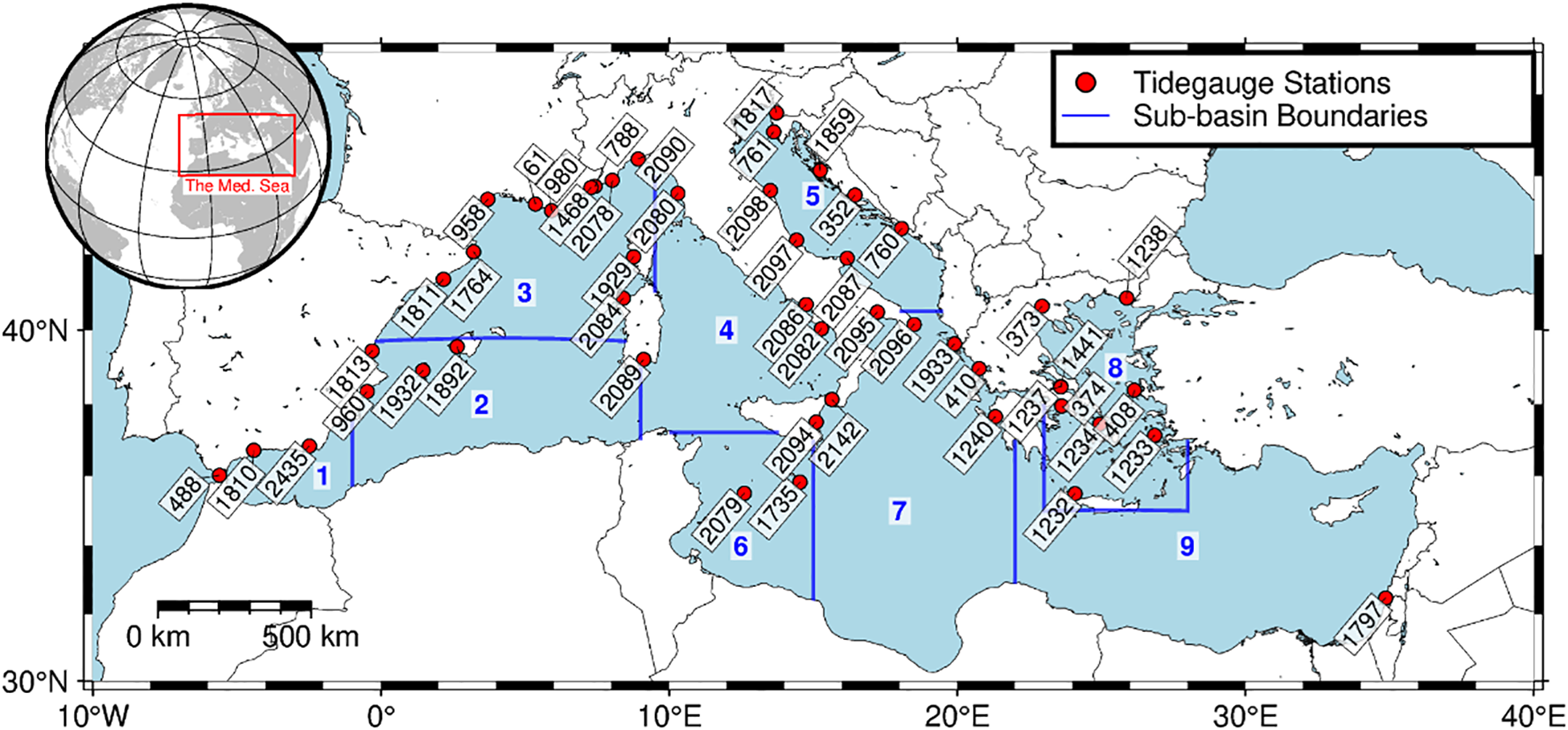
Locations and IDs of the TGs utilized in this study, where the Mediterranean's main sub-basins are also shown: 1. Alboran; 2. South-West Mediterranean; 3. North-West Mediterranean; 4. Tyrrhenian; 5. Adriatic; 6. Sicily Channel; 7. Ionian; 8. Aegean and 9. Levantine.
2.1.2 Vertical land motion data
The GNSS-related VLM was employed to adjust the TG trends. GNSS stations must be co-located with the TGs to ensure that the recorded VLM accurately reflects the measurements obtained from the TGs (Marcos et al., 2019). Particularly in areas with notable tectonic and human activity, the risk of different VLM between the GNSS and TG locations increases with their separation (Santamaría-Gómez et al., 2017). The VLM values employed to adjust the TG-derived relative sea-level time series were sourced from the Nevada Geodetic Laboratory (NGL). These data depend on the Median Interannual Difference Adjusted for Skewness (MIDAS, Blewitt et al., 2016; Hammond et al., 2021). VLM data were also obtained from the SONEL website, which relies on GNSS data from processing centers at the University of La Rochelle (ULR7, Gravelle et al., 2023).
We imposed an arbitrary maximum distance of 30 km for TG-GNSS (about 85% of stations were placed with less than 5 km) and a minimum data series duration of 10 years. This was done to improve the representativeness of the data incorporated in TG measurements. However, for some stations, these conditions were not met, so glacial isostatic adjustment (GIA)-related VLM derived from the gridded ICE-6G_C (VM5a) model by Peltier et al. (2015) was used. These data are accessible on the PSMSL website. Figure 2 illustrates the temporal availability of TG and GNSS-related VLM measurements at the designated sites.
Figure 2
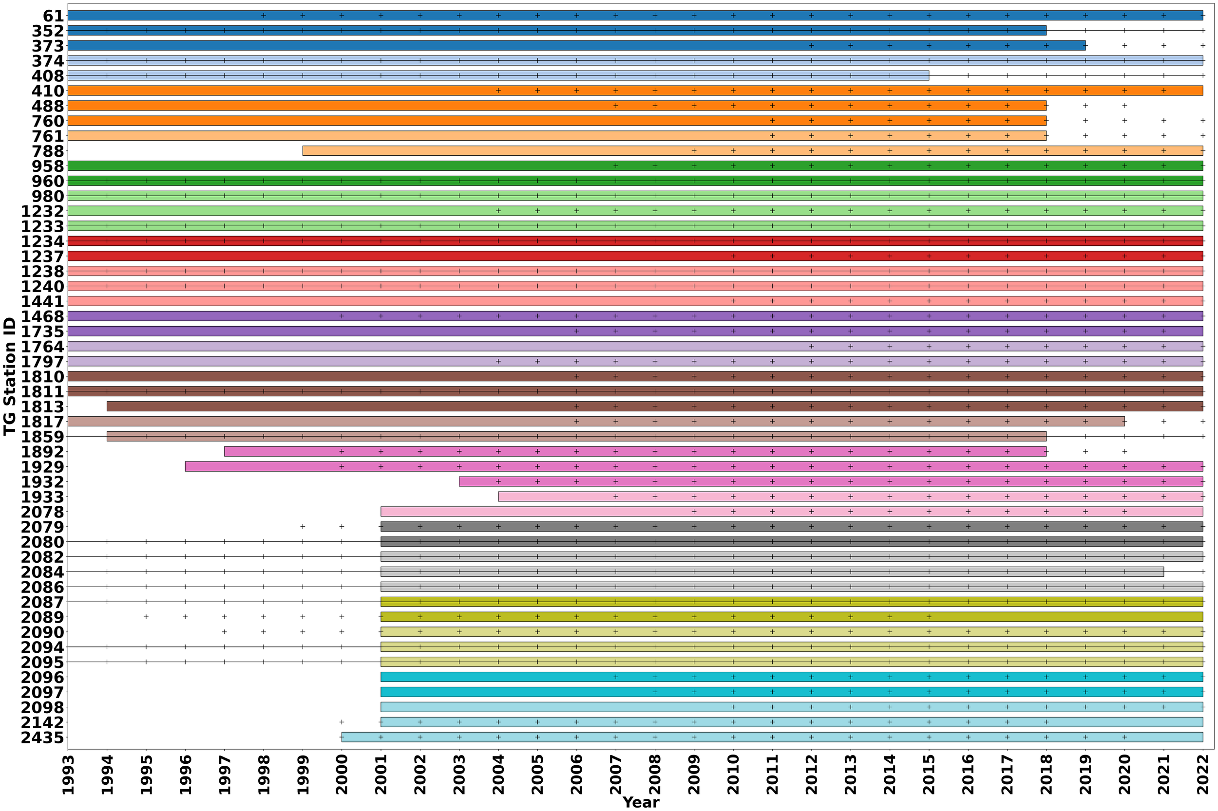
The details on TG's time availability (colored bars), GNSS-related VLM (black ' + '), and GIA-related VLM (Black line) data at the selected sites.
2.1.3 Altimetry data
Traditional satellite altimetry has developed into a technique for measuring ocean sea-level variations. This procedure was done by employing radar altimeters to ascertain sea surface height in relation to a reference ellipsoid (Frederikse et al., 2021). The coastal altimetry method is a specialized form of traditional satellite altimetry that focuses on assessing sea-level changes along the shoreline (Stammer and Cazenave, 2017; Wang and Huang, 2021; Kemgang Ghomsi et al., 2025). We considered two different coastal ALT datasets, hereby identified as X-TRACK-L2P and X-TRACK/ALES data.
The X-TRACK-L2P (1 Hz) data comprises along-track sea level anomalies (SLA) mapped onto reference tracks, with a spatial interval of approximately 6–7 km between points (1 second). The SLA time series has been generated using the X-TRACK processing system, utilizing Level 2 Plus (L2P) products provided by Aviso+. The altimetric corrections implemented are included in this product. The X-TRACK-L2P data relied on the T/P, Jason-1, 2, and 3, T/P interleaved, Jason-1 and 2 interleaved, ERS-1 and 2, ENVISAT, and SARAL/AltiKa missions spanning from 1993 to 2022 (Birol et al., 2017). In coastal zones, this technique works on modifying and post-processing the data. This practice improves the accuracy and completeness of sea surface height (SSH) measured by satellite altimetry (Birol et al., 2017).
The X-TRACK/ALES (2 Hz) data is a product of coastal sea levels along-track, provided for six designated zones by the sea-level project of the ESA's Climate Change Initiative (The Climate Change Coastal Sea Level Team 2020). This dataset is generated by predicting the satellite altimetry range with the "Adaptive Leading Edge Sub-waveform Retracker" (ALES, Passaro et al., 2014) and further processed utilizing the X-TRACK methodology (Birol et al., 2017; 2021). The X-TRACK/ALES data encompasses the three Jason-1, 2, and 3 missions from January 2002 to May 2018. The spatial resolution is 350 m at a frequency of 20 Hz, while the temporal resolution is 10 days (Bruni et al., 2022). Subsequently, this data was employed to investigate the ALT and TG measurement comparison zone of influence (Oelsmann et al., 2021), to observe sea-level changes on the West African coast (Marti et al., 2021), to assess sea-level changes along the coast of New Zealand (Erkoç and Doğan, 2023), and in the Mediterranean Sea region (Dieng et al., 2021; Bruni et al., 2022).
2.1.4 Virtual altimetry stations data
VAS does not correspond to physical locations on Earth, such as TG or meteorological stations. Rather, they represent virtual locations along satellite tracks from which researchers can obtain accurate sea level measurements by ALT (Cazenave et al., 2022). A VAS is created by the trajectory's closest distance to the seashore of the first valid point. This dataset is derived from reprocessed high-resolution (300 m) along-track ALT data collected during the Jason-1, Jason-2, and Jason-3 missions, which spanned from early 2002 to 2021 (Cazenave et al., 2022). Cazenave et al. (2022) reported SLA and corresponding coastal sea-level trends at more than 700 VAS situated along the global coasts, including the Mediterranean Sea, all within 6 km of the coast. Therefore, we utilized the VAS data to make up for the lack of TG stations along the African coast.
2.2 Data processing
2.2.1 Tide gauge data
To estimate sea-level trends depending on different techniques and to conduct a robust inter-technique comparison, it is essential to guarantee that the time series of the various observations achieve optimal consistency (Taibi and Haddad, 2019; Bruni et al., 2022). 49 TG stations were chosen after meeting the criteria mentioned in the dataset selection part. Then, the modified seasonal Mann-Kendall Test (MKT) was utilized. This test is a non-parametric statistical test employed to identify monotonic trends (either increasing or decreasing) in time series data. It modifies the calculation of the standard test's variance to account for the presence of serial correlation in the data (Hamed and Rao, 1998; Lornezhad et al., 2023). The null hypothesis (H0) in this test indicates that no trend exists in the data. This implies that the data are independently dispersed and random (Hamed and Rao, 1998; Taibi and Haddad, 2019).
For a data time series consisting of n points, denoted as x1, x2, …, xn, the MKT statistic (S) is calculated using Equations 1, 2, where S represents the difference between the number of increasing pairs and the number of declining pairs. A significant positive S implies an increasing trend, while a significant negative S denotes a decreasing trend (Hamed and Rao, 1998).
The seasonal MKT is a straightforward adaptation of the MKT that addresses observable seasonal variations in the dataset. This test conducts an independent MKT trend for each of the m distinct seasons, where m is the total number of seasons (Hirsch et al., 1982). The assessment involves calculating the MKT statistic (Si) and its variation Var (Si) for each season using measurements gathered throughout the years. The cumulative (S') and the cumulative Var (S') are derived by aggregating the S statistic for each season as shown in Equations 3, 4 (Hamed and Rao, 1998; Lornezhad et al., 2023).
The next step involves the most robust modification for the seasonal MKT, which utilizes a correction factor to account for serial correlation. The modified variance can be represented by Equation 5 (Hamed and Rao, 1998). The effective sample size represents the number of independent observations that are equivalent to the autocorrelated series. It is calculated as Equation 6 (Hamed and Rao, 1998; Lornezhad et al., 2023).
Where:
-
- n is the actual number of observations.
-
- is the autocorrelation function at lag k of the ranks of the data, not the original data itself. This is a crucial point.
Finally, the computation of the Z' statistics is calculated as Equation 7 (Hirsch et al., 1982; Hamed and Rao, 1998).
Evaluate ∣∣ against the crucial value α/2 from the standard normal distribution at a specified level of significance α (e.g., 0.05 for 95% confidence). If ∣∣> α/2, reject H0 (the trend is significant). The p-value can be obtained from Z; if the p-value is less than α, the trend is significant (Hirsch et al., 1982; Hamed and Rao, 1998; Lornezhad et al., 2023).
The modified seasonal MKT was conducted at a 5% level of significance for each dataset of the 49 TG stations. Subsequent to the test application, four time-series datasets were omitted: SOUDHAS station (ID 1232), ZADAR station (ID 1859), PALINURO station (ID 2082), and CATANIA II station (ID 2094), as indicated in Table 1. Consequently, 45 of the 49 stations are deemed acceptable following the test application, with all relevant application information shown in Table A in Supplementary Material.
Table 1
| Station ID. | Station name | S' | Var(S') standard | Var(S') modified | Z | P-value | Null hypothesis (H0) |
|---|---|---|---|---|---|---|---|
| 1232 | SOUDHAS | 374 | 40734 | 62819 | 1.488 | 0.13669 | Not rejected |
| 1859 | ZADAR | 47 | 16556 | 6297 | 0.580 | 0.56213 | Not rejected |
| 2082 | PALINURO | 374 | 40734 | 62819 | 1.488 | 0.13669 | Not rejected |
| 2094 | CATANIA II | 64 | 15014 | 7411 | 0.732 | 0.46429 | Not rejected |
The excluded TG stations after applying the modified seasonal Mann-Kendall test.
S' is the Seasonal Mann-Kendall statistic, Var(S') standard is its variation, and Var(S') modified is the modified variance which uses a correction factor to account for serial correlation. The (Equation 7) is utilized as an indicator of the trend's significance. The Null Hypothesis (H₀) in this test indicates that no trend exists in the data.
Following the application of the modified seasonal MKT to assess trends, the seasonal cycle was eliminated to detrend the time series. It was accomplished using the Multiple Seasonal Trend decomposition based on LOESS (MSTL) (Bandara et al., 2025). This method is commonly employed to separate time series of data into three parts: trend, seasonal, and residual, as delineated in Equation 8 (Bandara et al., 2025). Subsequently, the original trend was reintroduced into the deseasonalized time series.
where:
-
-Yt is the observed time series,
-
-Tt is the trend component,
-
-S1,t,S2,t,…, Sn,t are the seasonal components (one for each seasonal period),
-
-Rt is the remainder (residual) component.
In the absence of an error accompanying the data, trends are calculated utilizing the ordinary least squares (OLS) approach. This approach estimates the unknown parameters in a linear regression model (Zdaniuk, 2024). The objective is to identify the line (or hyperplane in higher dimensions) that optimally fits the data. That is done by reducing the total squared differences between the values that were observed and those that the model predicted as per Equation 9 (Leclercq et al., 2025).
where:
-
-Y is the dependent variable (response),
-
-x1, x2,…, xp are the independent variables (predictors),
-
-β0, β1,…, βp are the regression coefficients,
-
-ϵ is the error term (residuals).
The information about the accepted TG stations is shown in Table B in Supplementary Material. Figure 3 shows the monthly SLA and trends for the different stations over the period 1993–2022.
Figure 3
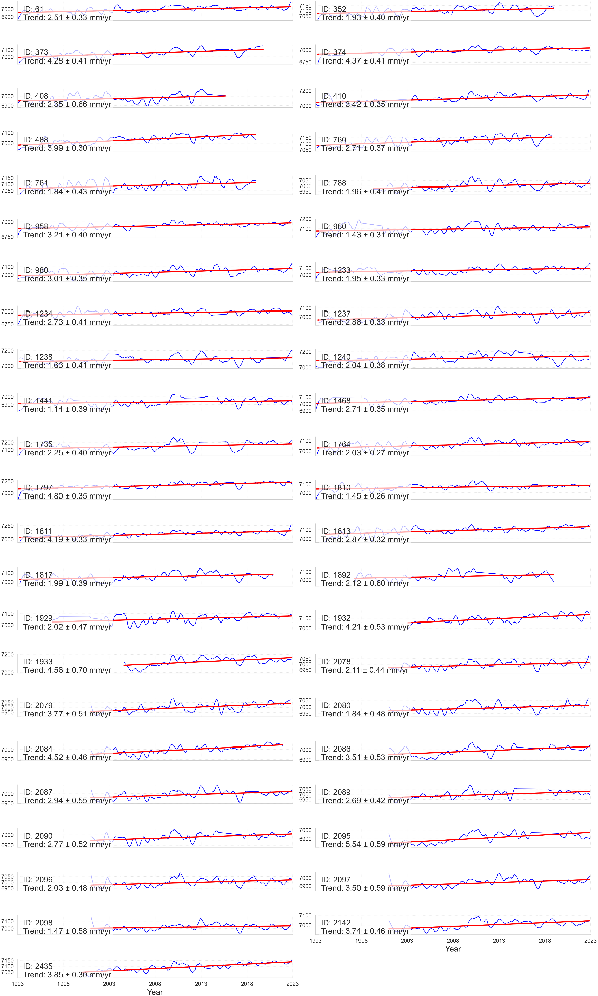
The monthly sea level anomalies and trends for the different stations over the period 1993–2022. Noted that the Y-axis of each subplot is the SLA in mm/year.
The TG time series were subsequently adjusted for the long-term impact of VLM, utilizing the trends obtained from GNSS data or GIA data (Kemgang Ghomsi et al., 2025) as per Equation 10.
where:
-
-ASL: Absolute Sea level
-
-RSL: Relative Sea level (Tide gauge data)
-
-VLM: Vertical Land Motion
The results demonstrate that intense VLM significantly influences sea-level trends along some sites on the northeast coast of the Mediterranean Sea. The large number of earthquakes that occurred in the Mediterranean region throughout the study period may account for the robust values of VLM. Seismic activity persists in the Mediterranean region, with 9,712 earthquakes of magnitude 4 or more documented from January 1993 to December 2022, as per the US Geological Survey (USGS) database. The US Geological Survey (USGS) database documented approximately 709 earthquakes with magnitudes of 5 or more during this extensive timeframe, and Figure 4 shows their locations. Consequently, we observe that regions frequently impacted by earthquakes influence sea level rise. This phenomenon is evident in locations such as DUBROVNIK (ID: 760) with a VLM of -1.57 mm/yr, KHALKIS NORTH (ID: 1237), and KHALKIS SOUTH (ID: 1441) with a VLM of 1.14 mm/yr (Figure 4).
Figure 4
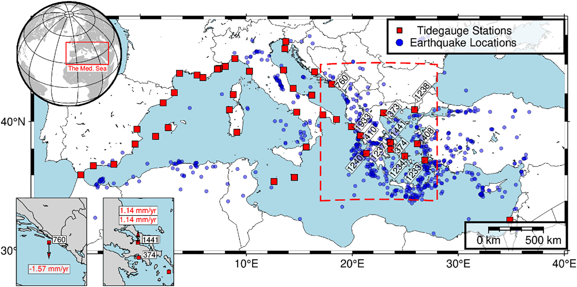
A map of the distribution of tide gauge (TG) stations and 709 earthquakes (M ≥ 5) in the Mediterranean Sea during the study period. An inset highlights the locations with high vertical land motion (VLM) values.
2.2.2 The X-TRACK-L2P altimetry data
The X-TRACK data, as detailed in Birol et al. (2017), is utilized in conjunction with AVISO L2P data. Equation 11 illustrates the computation of the SLA associated with the X-TRACK data.
The linear trends were calculated via the least-squares technique. The spatial distribution of sea level trends, shown in Figure 5, offers an explanation for the dynamic variations obtained from about thirty years of monthly mean ALT observations. The trends vary from −3 to 6 mm/year, indicating beneficial variations along the whole coastal zone of the Mediterranean Sea. These results match those conducted by Taibi and Haddad (2019). The highest value, 6 mm/year, recorded in certain areas on the coastlines, surpasses 1.8 times the present global average of 3.3 ± 0.3 mm/year reported by Guérou et al. (2023). This value indicates acceleration in SLR. The Adriatic, Aegean, and Levantine subbasins have the largest positive rates (4 mm/yr and higher), which matches the results by Calafat et al. (2022) and Meli et al. (2023). These high trends occur particularly in areas with recurrent gyres and eddies in circulation, such as the Shikmona Gyre System (SGS), the Pelops Gyre (PG), and the Mersa Matruh Gyre System (MMGS, Meli et al., 2023; Androulidakis and Pytharoulis, 2025). This observation is especially alarming as it exceeds worldwide forecasts and may result in accelerated coastal flooding, erosion, and the degradation of essential habitats. Conversely, some portions of the Levantine and Ionian sub-basins note negative trends (reaching -3 mm/yr) at considerable distances from the coastline. These adverse trends indicate limited oceanic phenomena, such as upwelling, alterations in dynamic topography, or sediment redistribution, rather than terrestrial influences (Kemgang Ghomsi et al., 2025).
Figure 5
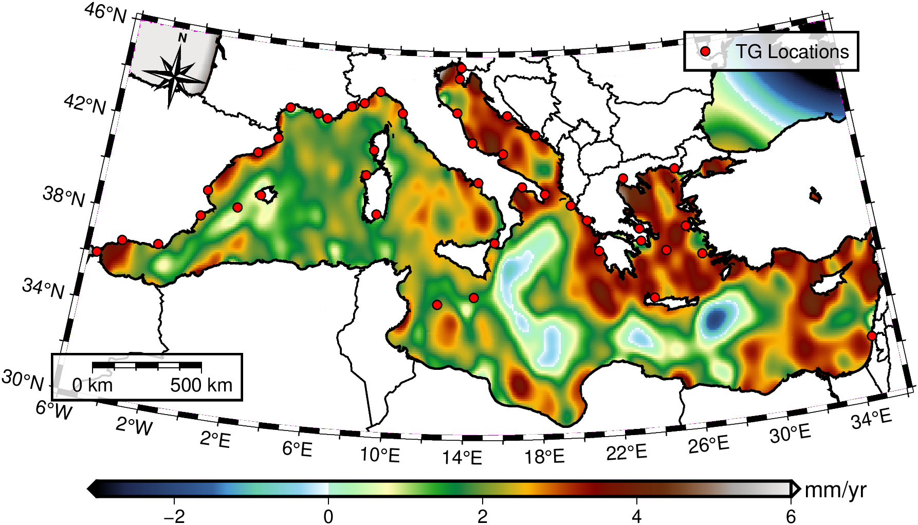
Sea-level trends (mm/yr) over the Mediterranean Sea calculated from X-TRACK-L2P data.
2.2.3 The X-TRACK/ALES dataset
Bruni et al. (2022) produced the X-TRACK/ALES dataset using algorithms and geophysical corrections refined for ALT observations of coastal areas. However, combining these data with in-situ data is not straightforward, as Jason's tracks do not always meet the TG sites. Consequently, TG and X-TRACK/ALES records may denote sites that are tens of kilometers apart. Therefore, a condition was established to select points from the dataset that are at maximum 40 kilometers apart from both the TG and the nearest location on any track. Thus, nine TG stations were chosen, and trends were calculated using the least squares technique. Figure 6 shows the tracks spanning the Mediterranean region, accompanied by the locations of the TGs incorporated in our analysis.
Figure 6
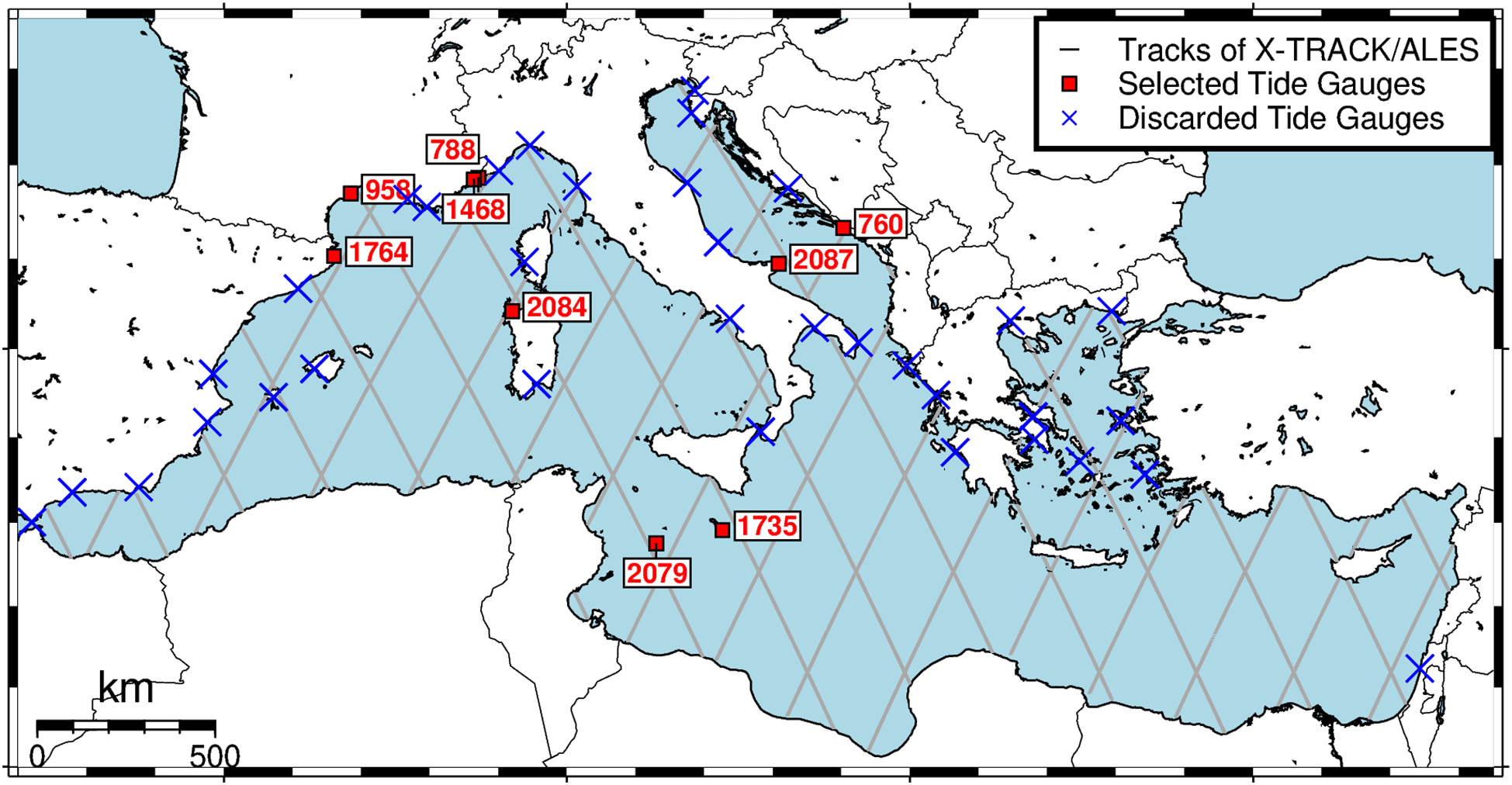
Map depicting the Jason missions' tracks (X-TRACK/ALES) across the Mediterranean basin (gray lines). Red squares indicate the TG sites chosen for the assessment. Cross-shaped markers denote the additional locations of TGs that were excluded (blue x).
3 Results and discussion
The sea-level trends of all selected TG stations were calculated based on Equation 10. All TG trends corrected to VLM have a statistically significant trend and show an increasing annual trend. Table B in Supplementary Material presents all the information about the TG data and their trend. The TARANTO II station (Station ID: 2095) has the highest yearly trend after the VLM adjustments, with a change rate of 5.281 mm/year. Conversely, the MALAGA II station (Station ID: 1810) exhibits the lowest yearly trend, of 0.696 mm/year. The mean trend across the stations is approximately 2.503 mm/year. This is consistent with the findings of Mohamed et al. (2019), who reported that the sea level in the Mediterranean has fluctuated at a rate of 2.5 mm/year from 1993 to 2017.
The rate of sea-level rise in some regions exceeds the global average of 3.3 mm/year reported by Guérou et al. (2023). These regions are THESSALONIKI (ID: 373) at 4.197 mm/year, PIRAIEVS (ID: 374) at 4.183 mm/year, TARIFA (ID: 488) at 3.319 mm/year, KHALKIS NORTH (ID: 1237) at 3.995 mm/year, HADERA (ID: 1797) at 5.034 mm/year, BARCELONA (ID: 1811) at 3.823 mm/year, CORFU (ID: 1933) at 3.886 mm/year, PORTO TORRES (ID: 2084) at 3.925 mm/year, TARANTO II (ID: 2095) at 5.281 mm/year, REGGIO CALABRIA II (ID: 2142) at 3.651 mm/year, and ALMERÍA (ID: 2435) at 3.819 mm/year. These results are in good agreement with the findings from the common TG stations studied by Bonaduce et al. (2016); Ramos-Alcántara et al. (2022), and Pandžić et al. (2024). It should be noted that variations in the time series period lead to differences of approximately 1 mm/year at a few sites. Figure 7 illustrates the linear trend of the TG time series, the values of VLM, and the adjusted trends corresponding to VLM along with their uncertainty.
Figure 7
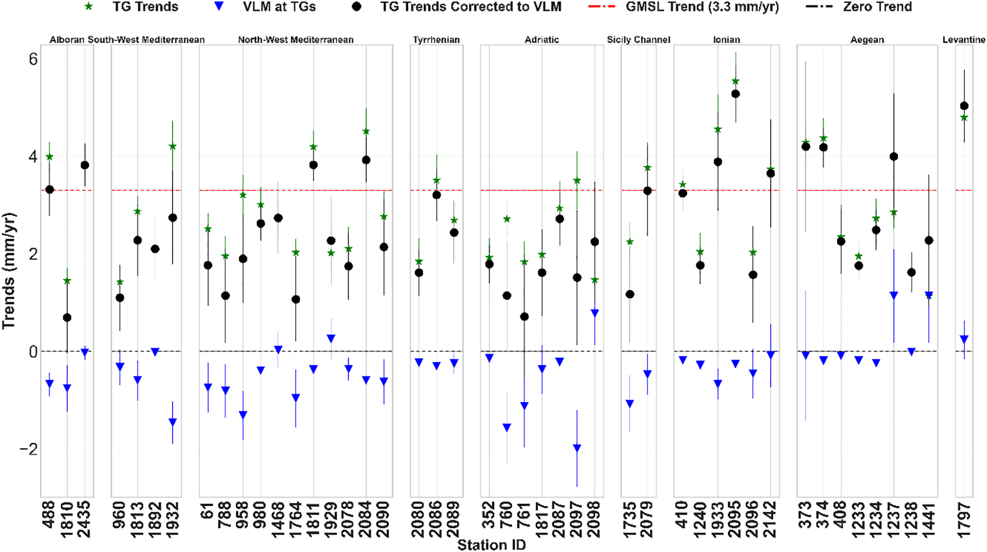
The values of TG trend, VLM, and the corrected trends to VLM with their uncertainties distributed according to sub-basins.
The trends obtained from the X-TRACK-L2P data were calculated for all 45 TGs. A comparison with the VLM-corrected TG trend was conducted, as illustrated in Table 2 and Figure 8.
Table 2
| Station ID. | Lat. (in Deg.) | Long. (in Deg.) | RSL (TG) | GNSS station name | Distance of TG-GNSS (km) | VLM | ASL | (RSL+VLM) versus ALT | |
|---|---|---|---|---|---|---|---|---|---|
| (RSL+VLM) | ALT | ||||||||
| 61 | 43.279 | 5.354 | 2.512 | MARS a | 0.007 | -0.743 | 1.769 | 2.367 | 0.598 |
| 352 | 43.507 | 16.442 | 1. 928 | (GIA) | —– | -0.140 | 1.788 | 2.822 | 1.034 |
| 373 | 40.633 | 22.935 | 4.283 | THS1 a | 2.142 | -0.086 | 4.197 | 3.429 | -0.768 |
| 374 | 37.937 | 23.627 | 4.373 | (GIA) | —– | -0.190 | 4.183 | 2.484 | -1.699 |
| 408 | 38.372 | 26.141 | 2.346 | (GIA) | —– | -0.090 | 2.256 | 3.239 | 0.983 |
| 410 | 38.959 | 20.757 | 3.423 | LFKD a | 14.355 | -0.180 | 3.243 | 2.681 | -0.562 |
| 488 | 36.009 | -5.603 | 3.989 | CEU1 b | 0.009 | -0.670 | 3.319 | 1.809 | -1.511 |
| 760 | 42.658 | 18.063 | 2.714 | DUB2 a | 3.96 | -1.567 | 1.147 | 2.722 | 1.575 |
| 761 | 45.083 | 13.628 | 1.837 | PORE a | 16.075 | -1.123 | 0.714 | 2.912 | 2.198 |
| 788 | 43.729 | 7.421 | 1.957 | EZEV a | 7.932 | -0.811 | 1.146 | 2.117 | 0.971 |
| 958 | 43.398 | 3.699 | 3.212 | SETE a | 0.006 | -1.312 | 1.9 | 2.847 | 0.947 |
| 960 | 38.339 | -0.481 | 1.429 | ALAC a | 0 | -0.327 | 1.102 | 2.013 | 0.911 |
| 980 | 43.113 | 5.915 | 3.012 | (GIA) | —– | -0.390 | 2.622 | 2.265 | -0.356 |
| 1233 | 37.13 | 26.848 | 1.95 | (GIA) | —– | -0.190 | 1.76 | 2.440 | 0.680 |
| 1234 | 37.44 | 24.946 | 2.729 | (GIA) | —– | -0.240 | 2.489 | 2.320 | -0.169 |
| 1237 | 38.472 | 23.593 | 2.856 | HALK a | 1.151 | 1.139 | 3.995 | 2.865 | -1.130 |
| 1238 | 40.844 | 25.878 | 1.633 | (GIA) | —– | -0.010 | 1.623 | 2.927 | 1.304 |
| 1240 | 37.645 | 21.32 | 2.045 | (GIA) | —– | -0.280 | 1.765 | 1.914 | 0.149 |
| 1441 | 38.461 | 23.589 | 1.138 | HALK a | 1.249 | 1.139 | 2.277 | 2.857 | 0.580 |
| 1468 | 43.696 | 7.286 | 2.709 | NICE a | 3.521 | 0.027 | 2.736 | 2.125 | -0.611 |
| 1735 | 35.82 | 14.533 | 2.248 | MALT a | 2.08 | -1.076 | 1.172 | 1.757 | 0.584 |
| 1764 | 42.054 | 3.206 | 2.03 | GIRO a | 29.117 | -0.961 | 1.069 | 2.647 | 1.578 |
| 1797 | 32.47 | 34.863 | 4.795 | CSAR a | 3.218 | 0.239 | 5.034 | 3.438 | -1.597 |
| 1810 | 36.712 | -4.417 | 1.451 | MLGA a | 1.689 | -0.755 | 0.696 | 2.082 | 1.386 |
| 1811 | 41.342 | 2.166 | 4.193 | (GIA) | —– | -0.37 | 3.823 | 2.635 | -1.188 |
| 1813 | 39.442 | -0.311 | 2.872 | VCIA a | 2.894 | -0.593 | 2.279 | 2.335 | 0.056 |
| 1817 | 45.548 | 13.725 | 1.985 | KOPE a | 0.001 | -0.369 | 1.616 | 2.904 | 1.288 |
| 1892 | 39.552 | 2.639 | 2.121 | MALL b | 0.875 | -0.020 | 2.101 | 1.751 | -0.350 |
| 1929 | 41.923 | 8.763 | 2.016 | AJAC a | 0.518 | 0.255 | 2.271 | 1.946 | -0.326 |
| 1932 | 38.911 | 1.45 | 4.205 | IBIZ a | 0.076 | -1.462 | 2.743 | 1.812 | -0.931 |
| 1933 | 39.628 | 19.905 | 4.556 | KASI b | 13.372 | -0.670 | 3.886 | 2.825 | -1.061 |
| 2078 | 43.878 | 8.019 | 2.106 | EZEV b | 0.767 | -0.360 | 1.746 | 2.093 | 0.347 |
| 2079 | 35.5 | 12.604 | 3.767 | LAMP a | 0.111 | -0.474 | 3.293 | 2.238 | -1.055 |
| 2080 | 43.546 | 10.299 | 1.845 | (GIA) | —– | -0.230 | 1.615 | 2.263 | 0.649 |
| 2084 | 40.842 | 8.404 | 4.515 | (GIA) | —– | -0.590 | 3.925 | 1.756 | -2.170 |
| 2086 | 40.677 | 14.751 | 3.507 | (GIA) | —– | -0.30 | 3.207 | 2.345 | -0.861 |
| 2087 | 41.888 | 16.177 | 2.938 | (GIA) | —– | -0.220 | 2.718 | 2.591 | -0.127 |
| 2089 | 39.21 | 9.114 | 2.689 | CAGL b | 1.891 | -0.250 | 2.439 | 1.687 | -0.752 |
| 2090 | 44.41 | 8.926 | 2.765 | GENO a | 1.086 | -0.624 | 2.141 | 1.988 | -0.153 |
| 2095 | 40.476 | 17.224 | 5.541 | (GIA) | —– | -0.260 | 5.281 | 3.630 | -1.651 |
| 2096 | 40.147 | 18.497 | 2.03 | GIUR a | 6.246 | -0.457 | 1.573 | 2.750 | 1.176 |
| 2097 | 42.356 | 14.415 | 3.503 | FRRA a | 12.214 | -1.988 | 1.515 | 2.468 | 0.954 |
| 2098 | 43.625 | 13.507 | 1.47 | ANCG a | 2.465 | 0.778 | 2.248 | 2.619 | 0.371 |
| 2142 | 38.122 | 15.649 | 3.736 | TGRC a | 1.498 | -0.085 | 3.651 | 1.796 | -1.855 |
| 2435 | 36.832 | -2.485 | 3.849 | ALME b | 0.002 | -0.030 | 3.819 | 2.245 | -1.575 |
Comparison between trends of corrected TG data and the X-TRACK 1 Hz trend (ALT) at the same locations (mm/year).
a is the VLM rate from NGL(MIDAS), while b is the VLM rate from SONEL (ULR7A).
Figure 8
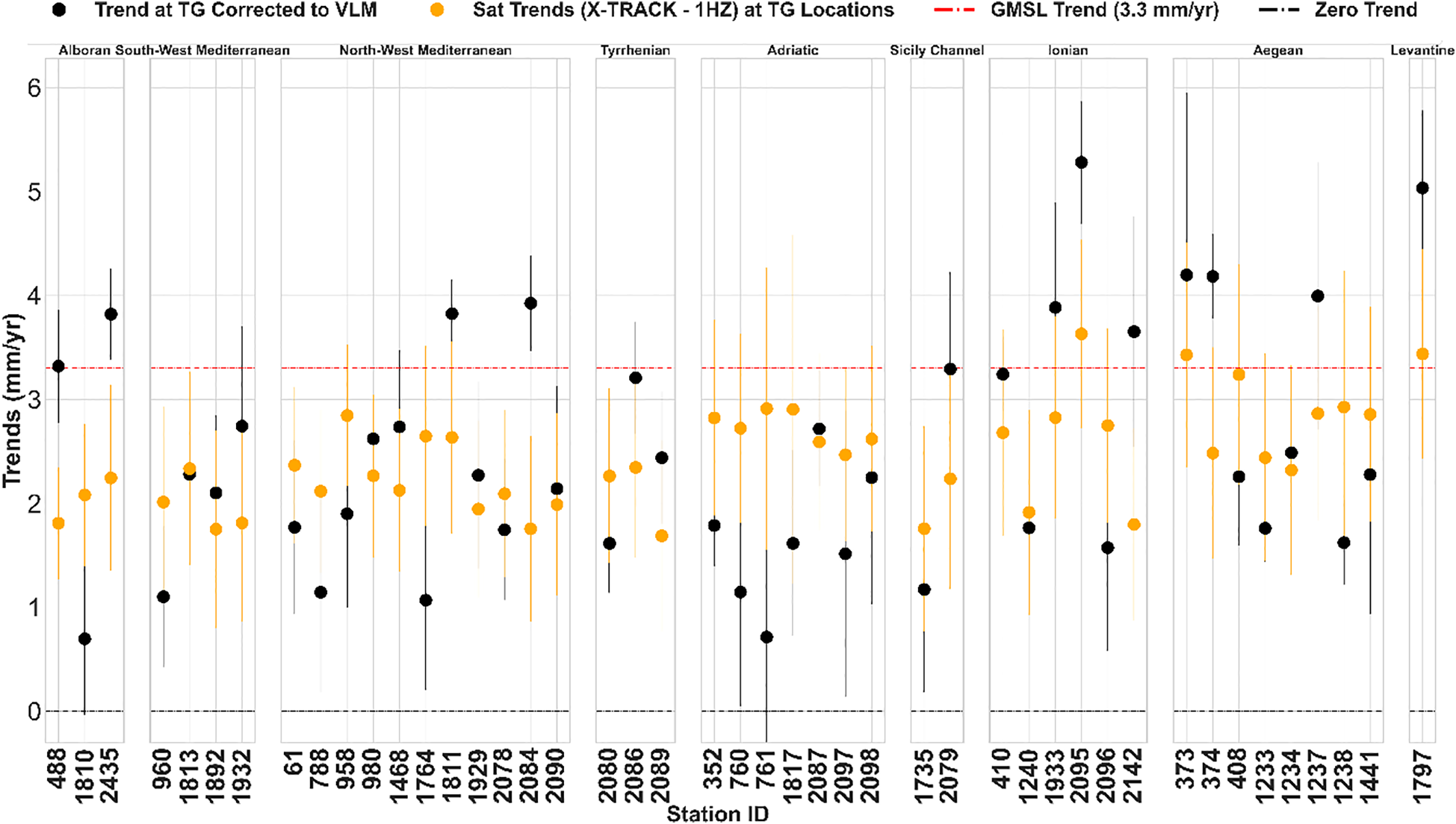
Values of sea level trends and uncertainties obtained from TG data (black circles) and X-TRACK-L2P data (orange circles) at TG locations distributed according to sub-basins.
The computed trends indicate positive linear trends in 1993–2022. Notably, higher rates of sea level increase were recorded in several locations, particularly THESSALONIKI (ID: 373), HADERA (ID: 1797), and TARANTO II (ID: 2095), where both TG records and X-TRACK-L2P data surpassed the world MSL trend. In some areas, such as the Aegean and Ionian seas, the rates of sea level rise significantly exceed the global mean. This pattern is consistent with the findings of Calafat et al. (2022), who addressed a high average rate of sea level rise across the entire Mediterranean Sea between 2000 and 2018.
Based on the values shown in Table 2, the statistics were calculated. The TG mean trend was 2.503 mm/year, and the TG standard deviation was 1.132. The ALT mean trend was 2.408 mm/year, and the ALT standard deviation was 0.529. In addition, the absolute discrepancies between rates from ALT and TG measurements ranged from 0.056 to 2.229 mm/year, with a mean of 0.095 mm/year. Finally, the root mean square error (RMSE X-TRACK-L2P) was 1.134. The discrepancies between X-TRACK-L2P and TG data are consistent with those derived from the Copernicus Marine Environment Monitoring Service (CMEMS) and VLM-corrected TG data analyzed by Bruni et al. (2022) and Hammond et al. (2021). These results sufficiently support the rising sea level over the Mediterranean Sea and the consistency between coastal sea level observations and in-situ data.
We also looked at whether the ALT product made for coastal use (X-TRACK/ALES) (20 Hz) matched better with TG observations than the X-TRACK-L2P (1 Hz) data. Therefore, as previously stated, we used the nearest point on the data track to determine the trend values at the TG locations. The sea-level trends were calculated for the selected nine points with approximately a complete time series of data. The minimum ALT-TG distance was 7.2 km at DUBROVNIK (ID: 760), and the maximum was 36.6 km at MARSAXLOKK (ID: 1735). To compare these trends with TG trends, the TG data had to be reanalyzed to match the XTRACK/ALES data period, which ran from 2002 to 2018. Table 3 displays the absolute values of the differences between the estimated trends from XTRACK/ALES data and in situ measurements at the nine sites.
Table 3
| Station ID. | Lat. (in Deg.) | Long. (in Deg.) | RSL (TG) | GIA-Related VLM | ASL | RSL+VLM versus ALT | |
|---|---|---|---|---|---|---|---|
| (RSL+VLM) | ALT (20Hz) | ||||||
| 760 | 42.658 | 18.063 | 2.051 | -0.14 | 1.911 | 1.704 | -0.207 |
| 788 | 43.729 | 7.421 | 1.835 | -0.29 | 1.545 | 0.293 | -1.253 |
| 958 | 43.398 | 3.699 | 2.479 | -0.23 | 2.249 | 0.858 | -1.390 |
| 1468 | 43.696 | 7.286 | 3.655 | -0.29 | 3.365 | 1.232 | -2.133 |
| 1735 | 35.820 | 14.533 | 2.923 | -0.51 | 2.413 | 1.999 | -0.413 |
| 1764 | 42.054 | 3.206 | 1.779 | -0.39 | 1.389 | 1.999 | 0.610 |
| 2079 | 35.500 | 12.604 | 3.047 | -0.36 | 2.687 | 0.288 | -2.399 |
| 2084 | 40.842 | 8.404 | 4.01 | -0.59 | 3.420 | 1.036 | -2.384 |
| 2087 | 41.888 | 16.177 | 4.045 | -0.22 | 3.825 | 3.030 | -0.795 |
Comparison between trends of corrected TG data to GIA-related VLM and the X-TRACK\ALES (ALT 20Hz) at the same locations (mm/year).
The statistics were calculated using data from 2002 to 2018. The TG mean trend was 2.534 mm/year, and the TG standard deviation was 0.862. While the ALT mean trend was 1.382 mm/year, and the ALT standard deviation was 0.893. In addition, the mean value of the differences between the trends from the two datasets was 1.152 mm/year, and the RMSE XTRACK/ALES was 1.517.
When comparing the trend differences between TG trends and both ALT datasets for the same nine sites (Figure 9), the X-TRACK-L2P data better matched the TG trends. This result may be due to the long measurement period of X-TRACK-L2P (from 1993 to 2022) and the corresponding TG records, which could better align with the SLR change (Bruni et al., 2022). This conclusion is also supported by its lower RMSE value for the nine stations (RMSEX-TRACK-L2P – 9 stations< RMSEX-TRACK/ALES). Therefore, the RMSE X-TRACK-L2P was recalculated for these nine TG datasets, giving a value of 1.144. However, X-TRACK/ALES exhibited even stronger trend agreement at only two sites: the in-site observations at DUBROVNIK (ID: 760), where the distance between TG and X-TRACK/ALES is smallest (about 7 km), which exactly matches Bruni et al. (2022) results. The second site is L'ESTARTIT (ID: 1764), which is about 20 km (Figure 9).
Figure 9
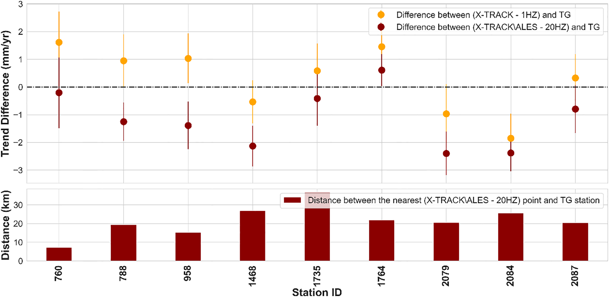
Comparison of TG records with X-TRACK/ALES data (20 Hz, red) and X-TRACK data (1 Hz, orange). For X-TRACK data (1 Hz), only the months included in the X-TRACK/ALES period were considered.
When comparing the trend differences derived from XTRACK/ALES and TG data with those concluded by Bruni et al. (2022), it became evident that the results are in agreement. The small discrepancies (approximately 0.5 mm/year) arise from applying more stringent selection criteria for TG stations, which require at least 18 years of data and 75% completeness, as well as a TG-GNSS distance of no more than 30 km. In contrast, Bruni et al. (2022) use less stringent TG selection criteria, requiring at least 14 years of data and 65% completeness.
Twenty-four VASs were used to estimate the change in sea level in the southern and eastern parts of the Mediterranean Sea to make up for the lack of TG stations. The trends of sea level were calculated using the least squares approach, depending on the values of monthly sea level anomalies provided for these stations. Furthermore, all the results show positive linear trends over the Mediterranean Sea, as shown in Figure 10. However, the issue with using the Virtual Altimetry Stations is their distance from the coast. That is because the first reliable points in the track that could be considered a VAS are located within 6 kilometers of the coast. Table C in Supplementary Material represents the information and trends on all the Virtual Altimetry Stations used in the study.
Figure 10
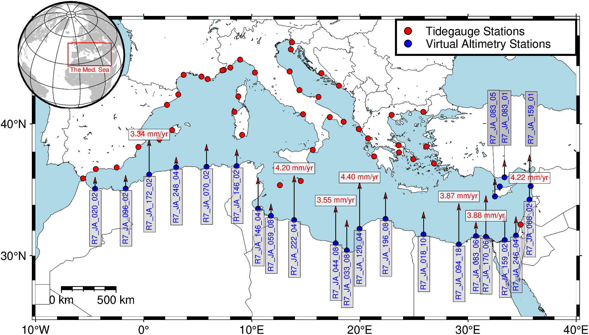
The locations of the virtual altimetry stations that were used in this study, where the red arrows represent the values of sea level trends.
Although several research studies advance our understanding of the dynamics of the Mediterranean Sea, they utilize different approaches and data sources. All of this investigation leads to complementary views about the positive linear trends of the Mediterranean Sea and its impacts on the coastal areas, but with slight differences in some results. However, some research, like Taibi and Haddad (2019), relied on a shorter time frame of the TG data while examining 18 high-quality tide-gauge stations from 1993 to 2015. Several investigations, such as Dieng et al. (2021), also utilized other Alt datasets, focusing only on validating the X-TRACK/ALES (20 Hz) product. In addition, Ramos-Alcántara et al. (2022) and Bruni et al. (2022) used CMEMS datasets. Furthermore, as noted in the dataset selection section, the station selection criteria in this study differ from those in earlier research. The stricter criteria applied here contribute to more accurate outcomes. Moreover, using a more updated dataset—which incorporates the X-TRACK-L2P product alongside X-TRACK/ALES, the longest available TG records (1993–2022) from 45 stations, and the VAS on the southern and eastern Mediterranean coastlines—enables a more robust and comprehensive assessment of three-decade trends across the entire Mediterranean basin.
Finally, it is noted that all the techniques used to calculate SLR rates in the Mediterranean Sea indicate positive linear trends. Some sites exhibit trends that surpass the global mean SLR, underscoring the necessity for proactive measures to address potential impacts of this phenomenon. The results also confirm the consistency of X-TRACK-L2P and TG data in representing the rates of SLR. For the southern and eastern coastline of the Mediterranean Sea, where no suitable tide gauge (TG) time series can be used, the X-TRACK-L2P or the VAS data can be relied upon. The RSL at any location without TG data can be estimated by subtracting the GNSS-related VLM from the ASL obtained from ALT data, provided that the closest GNSS station is used. If no nearby GNSS station is available, the GIA-related VLM can be used to correct the ALT data.
4 Impacts of SLR on Egypt
Rising sea levels, projected to cause flooding, are one of the most important challenges for the Mediterranean countries during this century (Grezio et al., 2025; Schuerch et al., 2025). According to scientists, up to 20 million people in the region could be permanently relocated by the end of the century if current trends in global warming and SLR continue (Hilmi et al., 2022). Egypt, located in northeastern Africa, shares its northern border with the Mediterranean Sea, as shown in Figure 11. Coastal regions at risk include Alexandria— a major industrial, commercial, urban center, and UNESCO World Heritage site on the Mediterranean—and the northern Nile Delta, where there is high population density. These areas face significant threats from coastal erosion and flooding driven by SLR (Hemeda, 2021; Grezio et al., 2025).
Figure 11
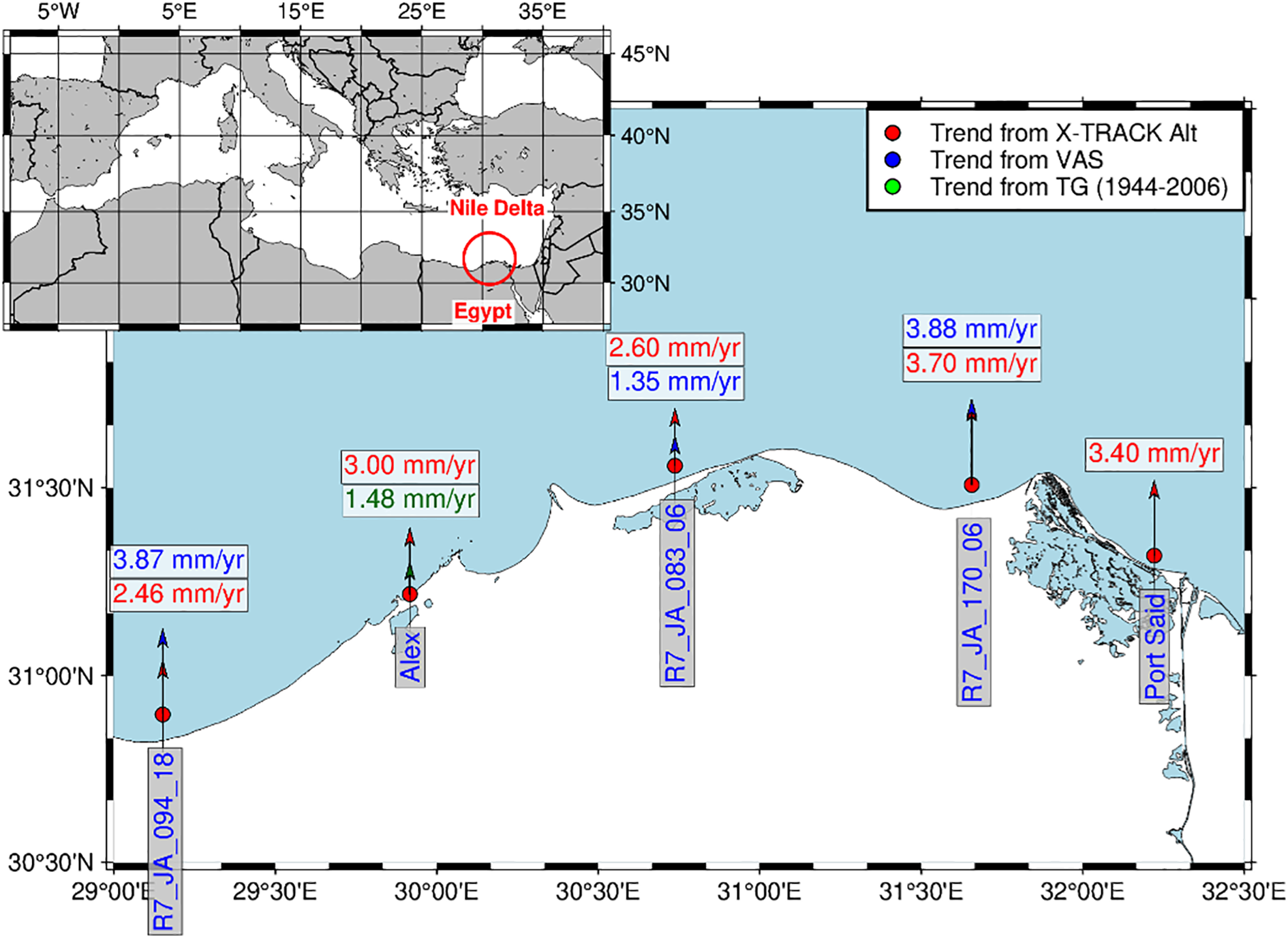
A map of Egypt's location with the sea level trends along the northern Delta coast.
Egypt's Nile Delta is regarded as the most significant of all, because it supports more than half of Egypt's agricultural land and is home to more than 50% of the country's people (Grezio et al., 2025). Delta's low-lying zones make up half of its total area. 2.4% of Egypt's land area is below 2 meters above mean sea level, making it especially susceptible to flooding, storms, and increasing sea levels (Shaltout et al., 2015; Hamzawy et al., 2023). A assessment from the International Panel on Climate Change (IPCC) states that rising sea levels, a consequence of global warming, are making Egypt's Nile Delta more susceptible to coastal flooding. According to the geospatial study that was done by Vecchio et al. (2024), the Mediterranean region's coastal plains have a total area of approximately 38,529 km² that could be vulnerable to flooding. France (3,681 km²), Italy (10,060 km²), and Egypt (12,879 km²) are the most affected nations. Allan et al. (2023) also note that by 2100, it is expected that 2,660 km² of the northern Delta will be underwater due to flooding (Vecchio et al., 2024).
According to Schuerch et al. (2025), the Nile Delta might lose thousands of acres suitable for investment, agriculture, or human habitation, with projections indicating a total loss of all coastal wetlands, even under optimistic climate change scenarios. Hamzawy et al. (2023) showed that sea levels in Egypt have risen by 3.2 mm annually since 2012, which will continue to flood and erode the Delta's northern shore. Our results indicate higher rates of sea level rise, with the Delta's sea level trend measuring 3.88 and 3.70 mm/year, respectively, based on the VAS and X-TRACK-L2P data (Figure 11).
Additionally, sea level rise will worsen saltwater intrusion, which will be hastened by rising temperatures and force saltwater into the groundwater and soil that farmers use for irrigation (Wassef and Schüttrumpf, 2016). The lakes and reclaimed lowlands in the Nile Delta depend on the sand belt, which can be destroyed by rising sea levels (Wassef and Schüttrumpf, 2016). Additionally, the Nile Delta may subside at a rate of 0.5 cm annually, hastening the process of Delta submergence (Rateb and Abotalib, 2020).
A similar issue is present in coastal cities like Alexandria (Radwan et al., 2021). Therefore, the rate of SLR in Alexandria (station ID: 503) was calculated using the PSMSL dataset for the period 1944-2006. After correction for GIA-related VLM, the SLR was estimated at 1.478 mm/year. For the shorter period 1993-2006, the SLR increased to 4.39 mm/year, indicating an acceleration in sea-level rise. In addition, the SLR was calculated from X-TRACK-L2P data, and it is estimated to be 3.00 mm/year (Figure 11), which exceeds the mean SLR in the Mediterranean Sea. According to experts, this is because the soil lacks silt, which solidifies the soil and is being held back more and more by the Nile Dam at Aswan, Upper Egypt. Therefore, everything related to water is at risk since rising sea levels brought on by global warming cause coastal cities to flood (Kamal et al., 2021).
Grezio et al. (2025) emphasize that sea-level rise, in conjunction with vertical land movement, exacerbates tsunami risks in the Mediterranean by elevating relative sea levels. Therefore, in Alexandria, residential and commercial properties are at risk of tidal, wind-driven, and storm surge flooding almost annually, and occasionally multiple times throughout the year, during times of intense rainfall, strong winds, and sea level rise (Hemeda, 2021).
At best, according to other Egyptian and UN studies, "30% of Alexandria will be flooded, 1.5 million or more people will be displaced, 195,000 jobs will be destroyed, and losses in land and construction will reach $30 trillion" if the Mediterranean rises just 50 centimeters (Hemeda, 2021). In addition to its history and its vestiges of the past, Alexandria is also home to the largest port in the country, which is the hub of the Egyptian economy; thus, the catastrophe will have an impact on approximately one hundred million Egyptians (Hemeda, 2021).
The Mediterranean is home to various UNESCO World Heritage Sites (WHS) that face threats from floods and erosion due to rising sea levels (Grezio et al., 2025). Reimann et al. (2018) assembled datasets that identify UNESCO cultural World Heritage Sites in the Mediterranean's Low-Elevation Coastal Zone (LECZ) as of 2018. Reimann et al. (2018) observed that several heritage sites, in regions facing sea level rise far beyond the global average, are particularly susceptible. Figure 12a shows the distribution of the UNESCO WHS on the Mediterranean coast. It also shows that several TG and VAS stations documented sea-level rise rates beyond the global mean where they are located in high population density areas. In addition, these stations are in proximity to multiple WHS, heightening the hazards of flooding and the potential loss of invaluable cultural landmarks. Furthermore, the historic coastal city of Alexandria in Egypt is facing increasing dangers that may result in the loss of cultural assets and substantial effects on tourism (Hemeda, 2021). Reimann et al. (2018) provide and illustrate all details about the Mediterranean UNESCO WHS, including their location in urban areas, site elevation, category, and distance from the coast.
Figure 12
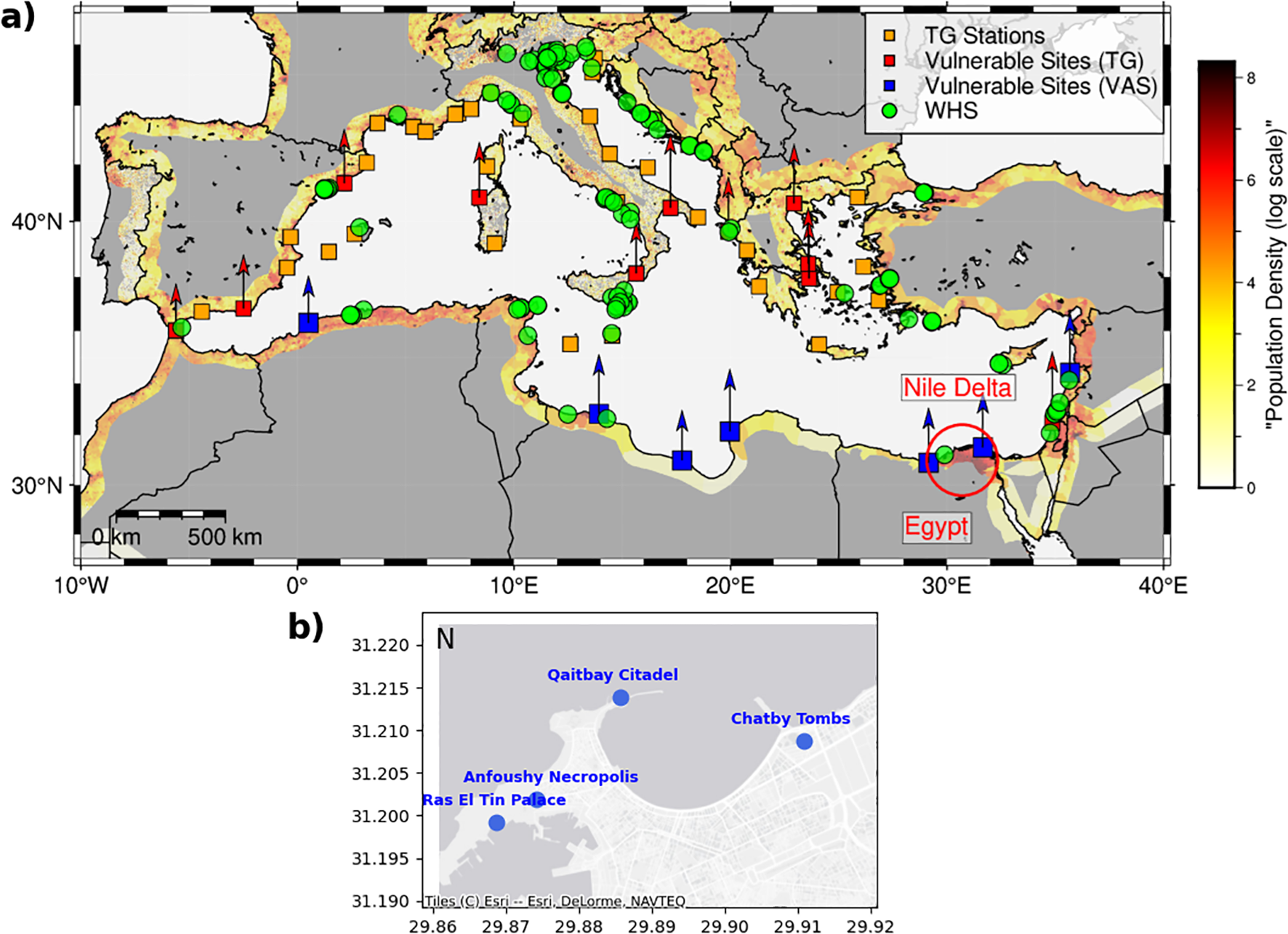
Map (a) illustrates World Heritage Sites (WHS) vulnerable to sea-level SLR and the distribution of population density along the Mediterranean coast (population data is from the Gridded Population of the World, Version 4). Map (b) provides a zoomed-in view of the heritage sites in Alexandria.
Numerous prior investigations, such as Frihy and El-Sayed (2013); Kamal et al. (2021), and Vousdoukas et al. (2022), demonstrated that Alexandria's coastal heritage sites will be impacted by sea inundation and disturbances in groundwater flow. These sites are low-lying archaeological locations such as the Qaitbay Citadel, Ras El Tin Palace, Chatby Tombs, and Anfoushy Necropolis. The four locations, as shown in Figure 12b, are situated at distances of about 25, 117, 180, and 300 meters from the sea, making them very susceptible to fluctuations in sea level (Kamal et al., 2021). The infiltration of seawater at these locations will also impact on the archaeological structures, thus necessitating the prompt implementation of essential protective actions.
5 Conclusion
Our findings emphasize the critical importance of understanding and monitoring sea level rise (SLR) along the Mediterranean coastline. In this region, SLR has been shaped by various processes, including the complex interplay between ocean circulation and climate variability. This study provides comprehensive information on sea-level variations along the Mediterranean coast between 1993 and 2022, utilizing a multifaceted methodology that incorporates both contemporary coastal ALT and TG data. It also demonstrates the agreement between these two techniques and emphasizes the implications of sea level rise (SLR) on Egypt's coastlines, using them as a case study.
We examined TG observations from the ALT era (1993–2022), which represents the longest period used in the analysis of TG data along the Mediterranean coast since satellite altimetry began. The network included 45 TG sites that provide time series spanning at least 18 years, with a minimum of 75% data completeness, and located within 30 kilometers of the nearest GNSS station. A modified seasonal Mann–Kendall test (MKT) was applied to detect significant patterns. Four TG datasets with otherwise suitable time series had to be excluded due to limitations in applying for the test. Sea-level trends, estimated using ordinary least squares (OLS) after removing the seasonal cycle with MSTL, showed rising sea levels at all TG sites with significant trends.
In our dataset, we established a maximum TG-GNSS distance of 30 km. In addition, a minimum data series duration of 10 years was set to improve the representativeness of the data included in TG measurements. Otherwise, we depended on GIA-related VLM. We observed that the sea level trends at certain locations on the northeast coast of the Mediterranean Sea are markedly affected by substantial vertical land movement (VLM). That brought us back to the significant frequency of earthquakes that occurred in the Mediterranean region, particularly in the Adriatic and Aegean sub-basins, during the research period. Upon rectifying the trends of TG to VLM, it was observed that all TG stations exhibit a statistically significant trend, characterized by an upward annual trajectory. The average trend among the stations is roughly 2.503 mm per year. Moreover, the rate of sea level increase in certain areas surpassed the global average of 3.3 mm/year, highlighting the pressing need for preventative actions to lessen the effects of SLR.
This study also confirmed the accuracy of coastal X-TRACK-L2P data by comparing it with TG records at selected sites. We mapped the regional distribution of sea-level trends from the X-TRACK-L2P dataset and their uncertainties. The trends ranged from −3 to 6 mm/year, showing notable variations across the Mediterranean coastline. Interannual variability revealed a strong correlation between coastal X-TRACK-L2P and TG data, with absolute differences of 0.056 to 2.229 mm/year (average of 0.095 mm/year), and the RMSEX-TRACK-L2P of 1.134. In several locations, SLR rates exceeded the global mean, particularly at THESSALONIKI (ID: 373), HADERA (ID: 1797), and TARANTO II (ID: 2095), where both TG and ALT values were above the global mean trend. Similarly, the Adriatic, Aegean, and Levantine subbasins also displayed SLR rates well above the global mean.
We also utilized the X-TRACK/ALES coastal data with only 9 TG stations located within 40 kilometers of the TG locations. The X-TRACK/ALES (20 Hz) trends were calculated for the 9 TGs, and a comparison with the VLM-corrected TG trend was also applied. It is noted that during the period (2002–2018), X-TRACK-L2P data exhibited superior concordance with in-situ data regarding the discrepancies between their trends than X-TRACK/ALES. However, TG and X-TRACK/ALES showed a higher level of agreement at only two locations, where the distances between TG locations and the closest point on the altimetry track were about 7 km and 20 km, respectively.
Concerning the southern and eastern Mediterranean coastline, we depended on the X-TRACK-L2P data, which has exhibited strong agreement with the TG data and the Virtual Altimetry Stations (VAS). Ultimately, all techniques employed to assess SLR rates in the Mediterranean Sea demonstrate positive linear trends, which points to the need for preventative actions to mitigate the SLR's possible effects.
Finally, we investigated the trend of sea level along Egypt's northern coast and noticed that it had risen above the Mediterranean Sea's mean, which threatens the low-lying zones of Egypt's Delta that are ideal for investment, agriculture, and human habitation. In addition, Alexandria's coastal heritage sites, particularly low-lying archaeological locations such as the Qaitbay Citadel, RAS ELTIN Palace, Chatby Tombs, and Anfoushy Necropolis, will be impacted by sea inundations and disturbances in groundwater flow.
Statements
Data availability statement
Publicly available datasets were analyzed in this study. The monthly tide-gauge time series are available from the PSMSL (https://psmsl.org/data/obtaining/). The vertical land motion values are sourced from the Nevada Geodetic Laboratory (NGL, https://geodesy.unr.edu/PlugNPlayPortal.php) using MIDAS velocities https://geodesy.unr.edu/velocities/midas.IGS14.txt), and from the SONEL website (https://www.sonel.org/-Vertical-land-movements-.html?lang=en). The utilization of GIA-related VLM derived from the gridded ICE-6G_C (VM5a) model, accessible on the PSMSL website (https://psmsl.org/train_and_info/geo_signals/gia/peltier/index.php). The X-TRACK-L2P SLA data was obtained from AVISO+ (https://www.aviso.altimetry.fr/en/data/products/sea-surface-height-products/regional/x-track-sla.html), while XTRACK/ALES data v1.1 are available at https://catalogue.ceda.ac.uk/uuid/222cf11f49a94d2da8a6da239df2efc4, https://doi.org/10.5270/esasl_cci-xtrack_ales_sla-200206_201805-v1.1-202006. The network of virtual altimetry stations v2.4 are available at https://www.seanoe.org/data/00631/74354/. The locations of UNESCO cultural World Heritage in the Mediterranean coastal zone are available at https://figshare.com/articles/dataset/UNESCO_cultural_World_Heritage_in_the_Mediterranean_coastal_zone/5759538. Finally, seismic activity locations in the Mediterranean region are obtained from the US Geological Survey (USGS) database (https://earthquake.usgs.gov/earthquakes/search/).
Author contributions
MY: Investigation, Conceptualization, Data curation, Writing – original draft, Visualization, Formal analysis, Methodology, Validation. QL: Writing – review & editing, Visualization, Investigation, Methodology, Data curation. AZ: Validation, Methodology, Data curation, Writing – review & editing. LW: Funding acquisition, Writing – review & editing, Methodology, Validation. LB: Investigation, Conceptualization, Writing – review & editing, Methodology, Supervision, Funding acquisition, Formal analysis.
Funding
The author(s) declare financial support was received for the research and/or publication of this article. This work was supported in part by the National Natural Science Foundation of China (Grant Nos. 42192535, 42174102, 42274116, 42404004) and the Natural Science Foundation of Wuhan (2024040701010065).
Acknowledgments
All data suppliers are appreciated by the authors. The authors also would like to thank the editor and the reviewers, whose comments and suggestions helped improve and clarify this manuscript.
Conflict of interest
The authors declare that the research was conducted in the absence of any commercial or financial relationships that could be construed as a potential conflict of interest.
Generative AI statement
The author(s) declare that no Generative AI was used in the creation of this manuscript.
Any alternative text (alt text) provided alongside figures in this article has been generated by Frontiers with the support of artificial intelligence and reasonable efforts have been made to ensure accuracy, including review by the authors wherever possible. If you identify any issues, please contact us.
Publisher’s note
All claims expressed in this article are solely those of the authors and do not necessarily represent those of their affiliated organizations, or those of the publisher, the editors and the reviewers. Any product that may be evaluated in this article, or claim that may be made by its manufacturer, is not guaranteed or endorsed by the publisher.
Supplementary material
The Supplementary Material for this article can be found online at: https://www.frontiersin.org/articles/10.3389/fmars.2025.1683307/full#supplementary-material
References
1
Allan R. P. Arias P. A. Berger S. Canadell J. G. Cassou C. Chen D. et al . (2023). “ Intergovernmental panel on climate change (IPCC). Summary for policymakers,” in Climate change 2021: The physical science basis. Contribution of working group I to the sixth assessment report of the intergovernmental panel on climate change (Cambridge, United Kingdom and New York, NY, USA: Cambridge University Press), 3–32. doi: 10.1017/9781009157896.001
2
Androulidakis Y. Pytharoulis I. (2025). Variability of marine heatwaves and atmospheric cyclones in the Mediterranean Sea during the last four decades. Environ. Res. Lett.20, 034031. doi: 10.1088/1748-9326/adb505
3
Bandara K. Hyndman R. J. Bergmeir C. (2025). MSTL: A seasonal-trend decomposition algorithm for time series with multiple seasonal patterns. Int. J. Oper. Res. 52 (1), 79–98. doi: 10.1504/IJOR.2025.143957
4
Bellas-Manley A. Nerem R. S. Hamlington B. D. (2025). Extrapolation of the satellite altimeter record to understand regional variations in future sea level change. J. Geophys. Res.: Oceans130, e2024JC022094. doi: 10.1029/2024JC022094
5
Birol F. Delebecque C. (2014). Using high sampling rate (10/20 Hz) altimeter data for the observation of coastal surface currents: A case study over the northwestern Mediterranean Sea. J. Mar. Syst.129, 318–333. doi: 10.1016/j.jmarsys.2013.07.009
6
Birol F. Fuller N. Lyard F. Cancet M. Nino F. Delebecque C. et al . (2017). Coastal applications from nadir altimetry: Example of the X-TRACK regional products. Adv. Space Res.59, 936–953. doi: 10.1016/j.asr.2016.11.005
7
Birol F. Léger F. Passaro M. Cazenave A. Niño F. Calafat F. M. et al . (2021). The X-TRACK/ALES multi-mission processing system: New advances in altimetry towards the coast. Adv. Space Res.67, 2398–2415. doi: 10.1016/j.asr.2021.01.049
8
Blewitt G. Kreemer C. Hammond W. C. Gazeaux J. (2016). MIDAS robust trend estimator for accurate GPS station velocities without step detection. J. Geophys. Res.: Solid Earth121, 2054–2068. doi: 10.1002/2015JB012552
9
Bonaduce A. Pinardi N. Oddo P. Spada G. Larnicol G. (2016). Sea-level variability in the Mediterranean Sea from altimetry and tide gauges. Climate Dyn.47, 2851–2866. doi: 10.1007/s00382-016-3001-2
10
Bruni S. Fenoglio L. Raicich F. Zerbini S. (2022). On the consistency of coastal sea-level measurements in the Mediterranean Sea from tide gauges and satellite radar altimetry. J. Geodesy96, 41. doi: 10.1007/s00190-022-01626-9
11
Calafat F. M. Frederikse T. Horsburgh K. (2022). The sources of sea-level changes in the Mediterranean Sea since 1960. J. Geophys. Res.: Oceans127, e2022JC019061. doi: 10.1029/2022JC019061
12
Cazenave A. Cozannet G. L. (2014). Sea level rise and its coastal impacts. Earth's Future2, 15–34. doi: 10.1002/2013EF000188
13
Cazenave A. Gouzenes Y. Birol F. Leger F. Passaro M. Calafat F. M. et al . (2022). Sea level along the world’s coastlines can be measured by a network of virtual altimetry stations. Commun. Earth Environ.3, 117. doi: 10.1038/s43247-022-00448-z
14
Dieng H. B. Cazenave A. Gouzenes Y. Sow B. A. (2021). Trends and inter-annual variability of altimetry-based coastal sea level in the Mediterranean Sea: Comparison with tide gauges and models. Adv. Space Res.68, 3279–3290. doi: 10.1016/j.asr.2021.06.022
15
Durand F. Piecuch C. G. Becker M. Papa F. Raju S. V. Khan J. U. et al . (2019). Impact of continental freshwater runoff on coastal sea level. Surveys Geophys.40, 1437–1466. doi: 10.1007/s10712-019-09536-w
16
Erkoç M. H. Doğan U. (2023). Monitoring of recently sea level changes on the coast of New Zealand using XTRACK coastal altimetry and tide gauge data. Continent. Shelf Res.269, 105127. doi: 10.1016/j.csr.2023.105127
17
Fox-Kemper B. (2021). “ Ocean, cryosphere and sea level change,” in AGU fall meeting abstracts, vol. 2021. New Orleans, LA, U13B–U109. doi: 10.1017/9781009157896.011
18
Frederikse T. Adhikari S. Daley T. J. Dangendorf S. Gehrels R. Landerer F. et al . (2021). Constraining 20th-century sea-level rise in the South Atlantic Ocean. J. Geophys. Res.: Oceans126, e2020JC016970. doi: 10.1029/2020jc01697
19
Frihy O. E. El-Sayed M. K. (2013). Vulnerability risk assessment and adaptation to climate change induced sea level rise along the Mediterranean coast of Egypt. Mitig. Adapt. Strateg. Global Change18, 1215–1237. doi: 10.1007/s11027-012-9418-y
20
Gravelle M. Wöppelmann G. Gobron K. Altamimi Z. Guichard M. Herring T. et al . (2023). The ULR-repro3 GPS data reanalysis and its estimates of vertical land motion at tide gauges for sea level science. Earth Syst. Sci. Data15, 497–509. doi: 10.5194/essd-15-497-2023
21
Grezio A. Anzidei M. Armigliato A. Baglione E. Maramai A. Selva J. et al . (2025). “ Tsunami hazard and risk in the Mediterranean Sea,” in Probabilistic Tsunami Hazard and Risk Analysis ( Elsevier), 397–415. doi: 10.1016/B978-0-443-18987-6.00015-4
22
Guérou A. Meyssignac B. Prandi P. Ablain M. Ribes A. Bignalet-Cazalet F. (2023). Current observed global mean sea level rise and acceleration estimated from satellite altimetry and the associated measurement uncertainty. Ocean Sci.19, 431–451. doi: 10.5194/egusphere-2022-330
23
Hamed K. H. Rao A. R. (1998). A modified Mann-Kendall trend test for autocorrelated data. J. Hydrol.204, 182–196. doi: 10.1016/S0022-1694(97)00125-X
24
Hammond W. C. Blewitt G. Kreemer C. Nerem R. S. (2021). GPS imaging of global vertical land motion for studies of sea level rise. J. Geophys. Res.: Solid Earth126, e2021JB022355. doi: 10.1029/2021JB022355
25
Hamzawy A. Al-Mailam M. Arkeh J. (2023). Climate change in Egypt: Opportunities and obstacles ( Carnegie Endowment for International Peace). Available online at: https://coilink.org/20.500.12592/6d61qd (Accessed June 25, 2025).
26
Hemeda S. (2021). Geotechnical modelling of the climate change impact on world heritage properties in Alexandria, Egypt. Heritage Sci.9, 73. doi: 10.1186/s40494-021-00547-8
27
Hilmi N. Ali E. Carnicer Cols J. Cramer W. Georgopoulou E. Le Cozannet G. et al . (2022). “ IPCC AR6 WGII cross-chapter paper 4: Mediterranean region,” in EGU General Assembly, Vienna, Austria, 23–27 May 2022, EGU22–10590. doi: 10.5194/egusphere-egu22-10590
28
Hirsch R. M. Slack J. R. Smith R. A. (1982). Techniques of trend analysis for monthly water quality data. Water Resour. Res.18, 107–121. doi: 10.1029/WR018i001p00107
29
Holgate S. J. Matthews A. Woodworth P. L. Rickards L. J. Tamisiea M. E. Bradshaw E. et al . (2013). New data systems and products at the permanent service for mean sea level. J. Coast. Res.29, 493–504. doi: 10.2112/JCOASTRES-D-12-00175.1
30
Jin Y. Chen M. Yan H. Wang T. Yang J. (2023). Sea level variation in the Arctic Ocean since 1979 based on ORAS5 data. Front. Mar. Sci.10. doi: 10.3389/fmars.2023.1197456
31
Kamal I. Fekri M. Abou El-Magd I. Soliman N. (2021). Mapping the impacts of projected sea-level rise on Cultural heritage sites in Egypt: Case study (Alexandria). J. Fac. Tour5, 1–20. doi: 10.21608/MFTH.2021.190350
32
Kemgang Ghomsi F. E. Erkoç M. H. Raj R. P. Pirti A. Bonaduce A. Abiodun B. J. et al . (2025). Sea level trends along the South African coast from 1993 to 2022 using XTRACK altimetry, tide gauges, and GNSS measurements. Sci. Rep.15, 4946. doi: 10.1038/s41598-025-89258-9
33
Leclercq L. Cazenave A. Leger F. Birol F. Nino F. Tolu L. et al . (2025). Coastal sea level rise at altimetry-based virtual stations in the Gulf of Mexico. Adv. Space Res.75, 1636–1652. doi: 10.1016/j.asr.2024.11.069
34
Legeais J. F. Meyssignac B. Faugère Y. Guerou A. Ablain M. Pujol M. I. et al . (2021). Copernicus sea level space observations: a basis for assessing mitigation and developing adaptation strategies to sea level rise. Front. Mar. Sci.8. doi: 10.3389/fmars.2021.704721
35
Li Y. Feng J. Yang X. Zhang S. Chao G. Zhao L. et al . (2024). Analysis of sea level variability and its contributions in the Bohai, Yellow Sea, and East China Sea. Front. Mar. Sci.11. doi: 10.3389/fmars.2024.1381187
36
Lornezhad E. Ebrahimi H. Rabieifar H. R. (2023). Analysis of precipitation and drought trends by a modified Mann–Kendall method: a case study of Lorestan province, Iran. Water Supply23, 1557–1570. doi: 10.2166/ws.2023.068
37
Marcos M. Wöppelmann G. Matthews A. Ponte R. M. Birol F. Ardhuin F. et al . (2019). Coastal sea level and related fields from existing observing systems. Surveys Geophys.40, 1293–1317. doi: 10.1007/s10712-019-09513-3
38
Marti F. Cazenave A. Birol F. Passaro M. Léger F. Niño F. et al . (2021). Altimetry-based sea level trends along the coasts of western Africa. Adv. Space Res.68, 504–522. doi: 10.1016/j.asr.2019.05.033
39
Masson-Delmotte V. Zhai P. Pirani A. Connors S. L. Péan C. Berger S. et al . (2021). “ Climate change 2021: the physical science basis,” in Contribution of working group I to the sixth assessment report of the intergovernmental panel on climate change 2, no. 1Cambridge, United Kingdom and New York, NY, USA: Cambridge University Press, 2391. doi: 10.1017/9781009157896
40
Meli M. Camargo C. M. Olivieri M. Slangen A. B. Romagnoli C. (2023). Sea-level trend variability in the Mediterranean during the 1993–2019 period. Front. Mar. Sci.10. doi: 10.3389/fmars.2023.1150488
41
Mohamed B. Abdallah A. M. Alam El-Din K. Nagy H. Shaltout M. (2019). Inter-annual variability and trends of sea level and sea surface temperature in the Mediterranean Sea over the last 25 years. Pure Appl. Geophys.176, 3787–3810. doi: 10.1007/s00024-019-02156-w
42
Oelsmann J. Calafat F. M. Passaro M. Hughes C. Richter K. Piecuch C. et al . (2024). Coherent modes of global coastal sea level variability. J. Geophys. Res.: Oceans129, e2024JC021120. doi: 10.1029/2024JC021120
43
Oelsmann J. Passaro M. Dettmering D. Schwatke C. Sánchez L. Seitz F. (2021). The zone of influence: matching sea level variability from coastal altimetry and tide gauges for vertical land motion estimation. Ocean Sci.17, 35–57. doi: 10.5194/os-17-35-202
44
Pandžić K. Likso T. Biondić R. Biondić B. (2024). A review of the contribution of satellite altimetry and tide gauge data to evaluate sea level trends in the Adriatic Sea within a Mediterranean and Global Context. GeoHazards5, 112–141. doi: 10.3390/geohazards5010006
45
Passaro M. Cipollini P. Vignudelli S. Quartly G. D. Snaith H. M. (2014). ALES: A multi-mission adaptive subwaveform retracker for coastal and open ocean altimetry. Remote Sens. Environ.145, 173–189. doi: 10.1016/j.rse.2014.02.008
46
Peltier W. R. Argus D. F. Drummond R. (2015). Space geodesy constrains ice age terminal deglaciation: The global ICE-6G_C (VM5a) model. J. Geophys. Res.: Solid Earth120, 450–487. doi: 10.1002/2014JB011176
47
Permanent Service for Mean Sea Level (PSMSL) (2025). Tide Gauge Data. Available online at: http://www.psmsl.org/data/obtaining/ (Accessed June 10, 2025).
48
Pinardi N. Bonaduce A. Navarra A. Dobricic S. Oddo P. (2014). The mean sea level equation and its application to the Mediterranean Sea. J. Climate27, 442–447. doi: 10.1175/JCLI-D-13-00139.1
49
Pinardi N. Zavatarelli M. Adani M. Coppini G. Fratianni C. Oddo P. et al . (2015). Mediterranean Sea large-scale low-frequency ocean variability and water mass formation rates from 1987 to 2007: A retrospective analysis. Prog. Oceanogr.132, 318–332. doi: 10.1016/j.pocean.2013.11.003
50
Puthucherril T. G. (2025). Adapting to sea level rise: Is India on- or off-track? Front. Mar. Sci.12. doi: 10.3389/fmars.2025.1516241
51
Radwan A. M. Magdy M. Rabah M. Saber A. Zaki A. (2021). Sea level analysis using tide gauge observations at the northern Delta coast, Egypt. NRIAG J. Astron. Geophys.10, 361–371. doi: 10.1080/20909977.2021.1940742
52
Ramos-Alcántara J. Gomis D. Jordà G. (2022). Reconstruction of Mediterranean coastal sea level at different timescales based on tide gauge records. Ocean Sci.18, 1781–1803. doi: 10.5194/os-18-1781-2022
53
Rateb A. Abotalib A. Z. (2020). Inferencing the land subsidence in the Nile Delta using Sentinel-1 satellites and GPS between 2015 and 2019. Sci. Total Environ.729, 138868. doi: 10.1016/j.scitotenv.2020.138868
54
Ray R. D. Loomis B. D. Zlotnicki V. (2021). The mean seasonal cycle in relative sea level from satellite altimetry and gravimetry. J. Geodesy95, 80. doi: 10.1007/s00190-021-01529-1
55
Reimann L. Vafeidis A. T. Brown S. Hinkel J. Tol R. S. J. (2018). Mediterranean UNESCO World Heritage at risk from coastal flooding and erosion due to sea-level rise. Nature communications9 (1), 4161. doi: 10.1038/s41467-018-06645-9
56
Rusu L. (2025). Climate change impact on the sea state conditions in the Mediterranean Sea under RCP and SSP emission scenarios. Renewable Energy243, 122616. doi: 10.1016/j.renene.2025.122616
57
Santamaría-Gómez A. Gravelle M. Dangendorf S. Marcos M. Spada G. Wöppelmann G. (2017). Uncertainty of the 20th century sea-level rise due to vertical land motion errors. Earth Planet. Sci. Lett.473, 24–32. doi: 10.1016/j.epsl.2017.05.038
58
Schuerch M. Kiesel J. Boutron O. Guelmami A. Wolff C. Cramer W. et al . (2025). Large-scale loss of Mediterranean coastal marshes under rising sea levels by 2100. Commun. Earth Environ.6, 128. doi: 10.1038/s43247-025-02099-2
59
Shaltout M. Tonbol K. Omstedt A. (2015). Sea-level change and projected future flooding along the Egyptian Mediterranean coast. Oceanologia57, 293–307. doi: 10.1016/j.oceano.2015.06.004
60
Stammer D. Cazenave A. (Eds.) (2017). Satellite altimetry over oceans and land surfaces (Boca Raton: CRC Press), 343–380. doi: 10.1201/9781315151779
61
Taibi H. Haddad M. (2019). Estimating trends of the Mediterranean Sea level changes from tide gauge and satellite altimetry data, (1993–2015). J. Oceanol. Limnol.37, 1176–1185. doi: 10.1007/s00343-019-8164-3
62
The Climate Change Coastal sea level team . (2020). ESA Sea Level Climate Change Initiative (Sea_Level_cci): Altimeter along-track high resolution sea level anomalies in some coastal regions (2002-2018) from the JASON satellites, v1.1. Centre for Environmental Data Analysis, date of citation. doi: 10.5270/esa-sl_cci-xtrack_ales_sla-200206_201805-v1.1-202005
63
Uzun P. Otay E. N. (2025). Sea-level change in Eastern Mediterranean, Aegean and Black seas analyzed at subregional scale of six CORDEX domains. Regional Stud. Mar. Sci.83, 104099. doi: 10.1016/j.rsma.2025.104099
64
Vecchio A. Anzidei M. Serpelloni E. (2024). Sea level rise projections up to 2150 in the northern Mediterranean coasts. Environ. Res. Lett.19, 014050. doi: 10.1088/1748-9326/ad127e
65
Vousdoukas M. I. Clarke J. Ranasinghe R. Reimann L. Khalaf N. Duong T. M. et al . (2022). African heritage sites threatened as sea-level rise accelerates. Nat. Climate Change12, 256–262. doi: 10.1038/s41558-022-01280-1
66
Wang J. Church J. A. Zhang X. Chen X. (2021). Reconciling global mean and regional sea level change in projections and observations. Nat. Commun.12, 990. doi: 10.1038/s41467-021-21265-6
67
Wang H. Huang Z. (2021). Waveform decontamination for improving satellite radar altimeter data over nearshore area: upgraded algorithm and validation. Front. Earth Sci.9. doi: 10.3389/feart.2021.748401
68
Wassef R. Schüttrumpf H. (2016). Impact of sea-level rise on groundwater salinity at the development area western Delta, Egypt. Groundwater Sustain. Dev.2, 85–103. doi: 10.1016/j.gsd.2016.06.001
69
Woodworth P. L. Melet A. Marcos M. Ray R. D. Wöppelmann G. Sasaki Y. N. et al . (2019). Forcing factors affecting sea level changes at the coast. Surveys Geophys.40, 1351–1397. doi: 10.1007/s10712-019-09531-1
70
Zdaniuk B. (2024). “ Ordinary least-squares (OLS) model,” in Encyclopedia of quality of life and well-being research ( Springer International Publishing, Cham), 4867–4869. doi: 10.1007/978-3-031-17299-1_2008
71
Zhou D. Liu Y. Feng Y. Zhang H. Fu Y. Liu Y. et al . (2022). Absolute sea level changes along the coast of China from tide gauges, GNSS, and satellite altimetry. J. Geophys. Res.: Oceans127, e2022JC018994. doi: 10.1029/2022JC018994
Summary
Keywords
tide gauge data, X-TRACK dataset, virtual altimetry stations, sea-level trends, the Mediterranean region, Egypt's low-lying coastal zones
Citation
Youssef MM, Li Q, Zaki A, Wu L and Bao L (2025) Estimating the Mediterranean sea-level trends from 1993 to 2022 showing the consistency of X-TRACK-L2P coastal altimetry with tide gauge data and trend impacts on Egypt's northern coast. Front. Mar. Sci. 12:1683307. doi: 10.3389/fmars.2025.1683307
Received
10 August 2025
Accepted
06 October 2025
Published
31 October 2025
Volume
12 - 2025
Edited by
David Alberto Salas de León, National Autonomous University of Mexico, Mexico
Reviewed by
Kreso Pandzic, Retired, Zagreb, Croatia; Muhammad Luqman Ahmad Affandi, Universiti Teknologi Malaysia, Malaysia
Updates
Copyright
© 2025 Youssef, Li, Zaki, Wu and Bao.
This is an open-access article distributed under the terms of the Creative Commons Attribution License (CC BY). The use, distribution or reproduction in other forums is permitted, provided the original author(s) and the copyright owner(s) are credited and that the original publication in this journal is cited, in accordance with accepted academic practice. No use, distribution or reproduction is permitted which does not comply with these terms.
*Correspondence: Lifeng Bao, baolifeng@apm.ac.cn
Disclaimer
All claims expressed in this article are solely those of the authors and do not necessarily represent those of their affiliated organizations, or those of the publisher, the editors and the reviewers. Any product that may be evaluated in this article or claim that may be made by its manufacturer is not guaranteed or endorsed by the publisher.