Abstract
Intensified ocean mixing can alter both the vertical temperature profile and biogeochemical states. Using a physical–biogeochemical coupled ocean model, we examine the impact of parameterized Langmuir circulation (LC) on the ocean carbon system in the Bering Sea. While LC has limited influence in summer, it significantly enhances turbulent mixing in winter, leading to an average wintertime mixed-layer deepening of about 11%. In the presence of a winter temperature inversion, LC-driven mixing enhances the entrainment of warmer subsurface water into the surface, increasing the surface ocean partial pressure of CO2 (pCO2). Concurrently, intensified vertical mixing entrains carbon-rich deep water into the surface layer, further elevating wintertime surface pCO2. By decomposing pCO2 into thermal and non-thermal components, we find that changes in dissolved inorganic carbon (DIC) supply exert a stronger influence than temperature-driven change, increasing the non-thermal pCO2 by up to 8.5 µatm in March and amplifying the seasonality of non-thermal processes. The thermal component also increases pCO2 by about 4.3 µatm in March, but its contribution to the seasonal amplitude is relatively small. These results demonstrate that enhanced vertical mixing combined with a winter temperature inversion can substantially alter pCO2 and air–sea CO2 fluxes in high-latitude regions; in regions without such inversions, thermal and non-thermal LC effects are likely to offset one another.
1 Introduction
The Bering Sea, a semi-enclosed marginal sea, is a corridor connecting the North Pacific to the Arctic. It can be divided into two regions by the shelf break with a distinct biogeochemical characteristics: a biologically active shelf to the northeast (Bates et al., 2011; Springer et al., 1996) and a High-Nutrient Low-Chlorophyll basin to the southwest (Tyrrell et al., 2005; Shiomoto et al., 2002). These regions show contrasting patterns in air-sea CO2 exchange - the shelf acts as a net annual sink of atmospheric CO2, whereas the basin serves as a net source (Zhang et al., 2023). In addition to spatial heterogeneity, the region exhibits strong seasonal variability, particularly in sea surface temperature (SST) (Shevchenko et al., 2024) and mixed layer depth (MLD) (Hayden and O’Neill, 2024; Johnson and Stabeno, 2017).
These seasonal changes drive biogeochemical temporal processes, influencing the seasonal variability of air-sea CO2 fluxes. Observation-based estimates indicate that the subpolar region of the North Pacific acts as a source of CO2 to the atmosphere in winter and a sink in summer (Rodgers et al., 2023), consistent with findings in the Bering Sea, where estimates reveal seasonal CO2 flux variability linked to changes in SST, MLD, and chlorophyll-a (Zhang et al., 2023). Many ocean biogeochemical models, however, struggle to accurately capture this seasonal cycle (McKinley et al., 2006; Lerner et al., 2021; Rodgers et al., 2023; Carroll et al., 2020). For instance, Lerner et al. (2021) reported that the NASA-GISS model simulates a seasonal CO2 flux pattern opposite to that inferred from observations. Similarly, most CMIP6 models reproduce reversed seasonal CO2 fluxes in the subpolar North Pacific (Rodgers et al., 2023). This misrepresentation also persists in data assimilation products that incorporate both physical and biogeochemical observations. Despite generally good agreement with observed fluxes globally, they fail to reproduce the correct seasonal CO2 exchange in this region (Carroll et al., 2020), likely due to unresolved physical processes that affect upper-ocean biogeochemistry.
Refinements in physical processes within ocean models can improve biogeochemical simulations. Multiple physical drivers influence the air-sea CO2 exchange, including mesoscale features resolved by high-resolution ocean models (Guo and Timmermans, 2024; Ford et al., 2023; Kim et al., 2022), freshwater-driven stratification (Ahmed et al., 2020; Dong et al., 2021), SST changes linked to marine heatwaves (Edwing et al., 2024), topographically modulated upwelling (Fiechter et al., 2014), and current-wind interaction (Kwak et al., 2021). In particular, surface vertical mixing can have a significant impact on air-sea CO2 flux. For example, vertical mixing induced by near-inertial waves can enhance DIC concentrations, thereby decreasing the CO2 uptake in austral summer (Song et al., 2019). In contrast, Langmuir turbulence contributes to enhanced carbon uptake, adding approximately 0.07–0.1 PgC/year of extra CO2 absorption globally (Smith et al., 2018). Tak et al. (2023) applied a LC parameterization to an ocean model in the Southern Ocean and showed deepening of the mixed layer, increasing sea-ice fraction, and improving the simulation of air–sea CO2 flux.
We hypothesize that the bias in the Bering Sea’s air–sea CO2 exchange may stem from biases in vertical mixing. Enhanced vertical mixing can influence CO2 flux through both thermal and non-thermal processes. Thermally, mixing tends to lower SST by bringing cooler subsurface water to the surface, which decreases surface pCO2. Non-thermally, mixing can elevate surface DIC concentrations by entraining DIC-rich subsurface water, which increases surface pCO2. These opposing effects can offset each other, which dampens net change on air–sea CO2 exchange. However, in high-latitude regions such as the Bering Sea, where wintertime thermal inversions are present (i.e., subsurface waters are warmer than the surface), LC-driven enhanced vertical mixing may produce a distinct effect on CO2 exchange.
This study evaluates the impact of LC parameterization on air–sea CO2 exchange in the Bering Sea using a physical-biogeochemical coupled model. As a first step, we decompose pCO2 into thermal and non-thermal components, clarifying the relative contributions of temperature-driven and biogeochemical processes. Next, we conduct a DIC budget analysis to investigate the mechanisms driving DIC changes under LC parameterization and to determine when and why LC-enhanced vertical mixing affects DIC redistribution and air–sea CO2 exchange.
2 Method
2.1 Langmuir circulation parameterization
LC refers to wind-driven, counter-rotating vortices aligned parallel to the wind direction (Langmuir, 1938). This circulation can erode near-surface stratification and thereby enhance vertical mixing in the upper ocean (Thorpe, 2004). The impact of LC on vertical mixing has been investigated using Large Eddy Simulations (LES), which show significant effects under weakly stratified conditions (Noh et al., 2011). To account for these effects in coarse-resolution global ocean models, LC has been parameterized and incorporated into global climate models, resulting in improvements such as the mitigation of the shallow mixed layer bias, especially in the Southern Ocean (Noh et al., 2016; Tak et al., 2023).
Ocean models typically incorporate LC by extending vertical mixing schemes. A commonly employed approach parameterizes LC effects in the K-profile parameterization (KPP) by increasing the turbulent velocity scale (McWilliams and Sullivan, 2000; Smyth et al., 2002; Li et al., 2016; Reichl et al., 2016). Additionally, LC effect is parameterized in the energetics-based planetary boundary layer (ePBL) scheme by enhancing the entrainment buoyancy flux (Reichl and Li, 2019). In this study, the influence of LC on the air-sea CO2 flux is investigated using a simple parameterization scheme presented in Tak et al. (2023). This LC parameterization modifies the turbulent kinetic energy (TKE) closure scheme by Gaspar et al. (1990) and Blanke and Delecluse (1993) where the vertical eddy viscosity is proportional to the turbulent mixing length scale (lmix) and the square root of the TKE. The LC parameterization relaxes the near-surface constraint on lmix by a factor of Γ (from local depth (z) to Γz), allowing larger lmix near the surface to represent LC-enhanced vertical mixing. Γ is shown to depend on the Langmuir number (Γ increases as La decreases), where and are the friction velocity and the Stokes velocity at the surface, respectively (McWilliams et al., 1997). Belcher et al. (2012) reported that La is smaller than 0.35 roughly 70% of the time during the Northern Hemisphere winter (around 60% in summer). Also based on LES results, Figure 8 of Noh et al. (2011) shows that the amplification of the mixing length scale under Langmuir circulation is well represented by Γ = 10 when La = 0.32. Therefore, we use La = 0.32 and Γ = 10 as constant values following Noh et al. (2011, 2016), and Tak et al. (2023), which provide a reasonable and practical approximation for implementing LC effects under our wintertime Bering Sea conditions.
This scheme also includes the effects of Stokes drift into both the TKE equation and the Coriolis term in the momentum equation (Tak et al., 2023). The magnitude of this contribution depends on the vertical profile of the Stokes velocity, , which is formulated as . The surface Stokes velocity is estimated using the Langmuir number, , and the friction velocity, , where is the wind stress and is the water density. The wavelength of the monochromatic surface wave, m, is adopted following Noh et al. (2004).
2.2 Model configuration
The impact of LC on air-sea CO2 flux in the Bering Sea is investigated using a global ocean configuration of the Massachusetts Institute of Technology general circulation model (MITgcm) (Adcroft et al., 1997, 2004; Marshall et al., 1997b, a, 1998). This configuration has a horizontal resolution of approximately 1° and shares many features with ECCO Version 4 (Forget et al., 2015). However, it includes key modifications, such as three additional vertical layers within the top 10 m of the ocean to better represent the effects of the LC parameterization.
The carbon cycle and air-sea CO2 flux are represented by the DIC module, a simple biogeochemical model that simulates 6 tracers: DIC, alkalinity, dissolved organic phosphorus, phosphate, oxygen, and iron (Dutkiewicz et al., 2005; Parekh et al., 2005; Song et al., 2016a, 2019). The air-sea CO2 flux () is given by
In Equation 1, kw is the piston velocity for CO2 weighted by the fraction of the sea-ice-free area within each grid cell. is the partial pressure of CO2 in the surface ocean, which is determined by local values of DIC, alkalinity, SST and sea surface salinity (SSS). The atmospheric partial pressure of CO2 () is prescribed as a fixed pre-industrial value of 278 µatm. Because is held constant, the surface ocean pCO2 controls the direction of the air-sea CO2 exchange (positive sign indicates oceanic uptake), and its magnitude depends on both kw and ΔpCO2. The surface DIC has two additional source/sink terms. The first accounts for changes due to biological production, estimated from phosphate consumption, which is converted to carbon consumption using the Redfield ratio. The second is the export of carbon to depth in the form of calcium carbonate shells. The biological production requires sunlight and nutrients, where sunlight exponentially decreases with depth and is further reduced by self-shading. Detailed information on the biological model configuration is available in the previous modeling study by Song et al. (2016b).
This physical-biogeochemical coupled model was first spun up for 600 years starting from the initial temperature, salinity and phosphate fields from World Ocean Atlas (https://www.nodc.noaa.gov/OC5/WOA09/pubwoa09.html), and DIC and alkalinity fields from GLODAP (Key et al., 2004) under the atmospheric forcing from Common Ocean-ice Reference Experiments version 2 (CORE-II) - “normal year” forcing dataset (Large and Yeager, 2004), which provides a repeat annual cycle representative of climatological conditions, and atmospheric iron deposition data from aeolian dust sources (Luo et al., 2008). The simulation bifurcates into two experiments after the spin up. The first experiment extends the simulation for an additional 100 years, serving as a baseline control (CTRL) where LC effects are excluded. The second experiment integrates 100 years with the LC parameterization to examine its impact on the air-sea CO2 exchange. A detailed description of the experimental setup can be found in Section 3 of Tak et al. (2023). For the analysis presented here, model outputs from the final nine years of each simulation were averaged.
3 Results
3.1 Air-sea carbon exchange
We first describe the annually averaged air-sea CO2 exchange in the Bering Sea. Figure 1 shows the annual mean in the Bering Sea, where the region is divided into the basin (deeper than 200 m) and shelf areas. The observation-based estimate of ΔpCO2, derived from the self-organizing map feed-forward neural network (SOMFFN) approach (Jersild et al., 2017), suggests that the basin tends to emit CO2, whereas the shelf takes up CO2 (Figure 1A). The CTRL captures the basin-shelf contrast in pCO2, and localized outgassing occurs in parts of the basin, but CO2 uptake dominates overall (Figure 1C). This bias is reduced by incorporating LC effect, which eventually decreases CO2 uptake, particularly in the western part of the basin (Figures 1B, D). Therefore, we focus on the basin region.
Figure 1
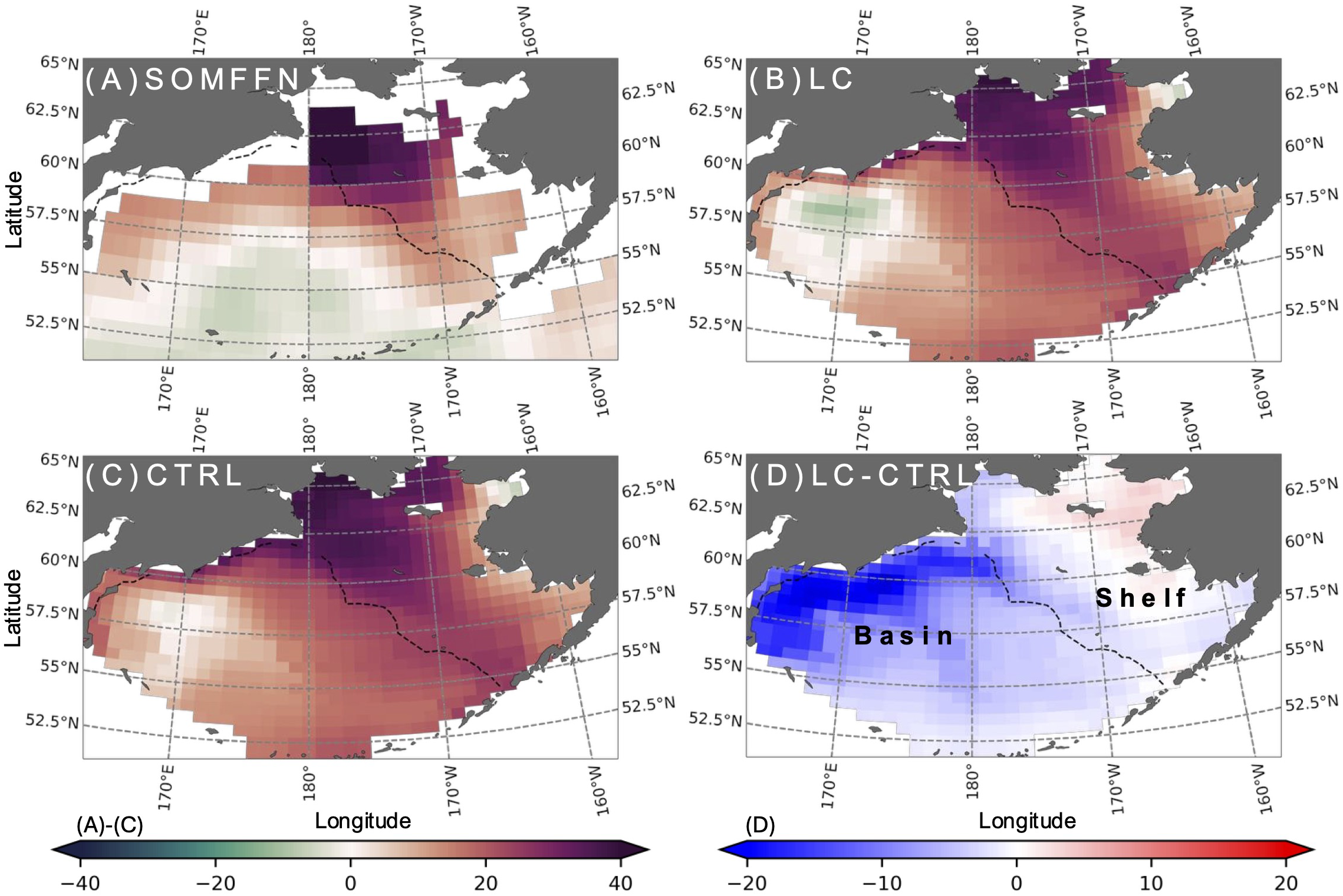
Annual mean for (A) SOMFFN, (B) LC, (C) CTRL and (D) LC minus CTRL. The black dashed line denotes the 200 m isobath.
This improvement can be attributed to enhanced vertical mixing by the LC effect. Compared with the MLD climatology dataset v2023 (de Boyer Montégut et al., 2004; de Boyer Montégut, 2023), CTRL has a shallower MLD bias in the basin, which is mitigated in the LC simulation (Supplementary Figure S1). This deepening results from increased turbulent mixing due to the inclusion of the LC effect. The LC parameterization is expected to enhance the lmix near the surface under weakly stratified conditions (Noh et al., 2016). Indeed, lmix is significantly amplified in the LC simulation, particularly during winter and early spring, showing an increase of approximately 44% near 100 m compared to CTRL (Figure 2C). Consistent with this, the increase in TKE is also more pronounced during winter and early spring, extending beyond 100 m (Figure 2F), suggesting deeper and more sustained vertical mixing due to LC.
Figure 2
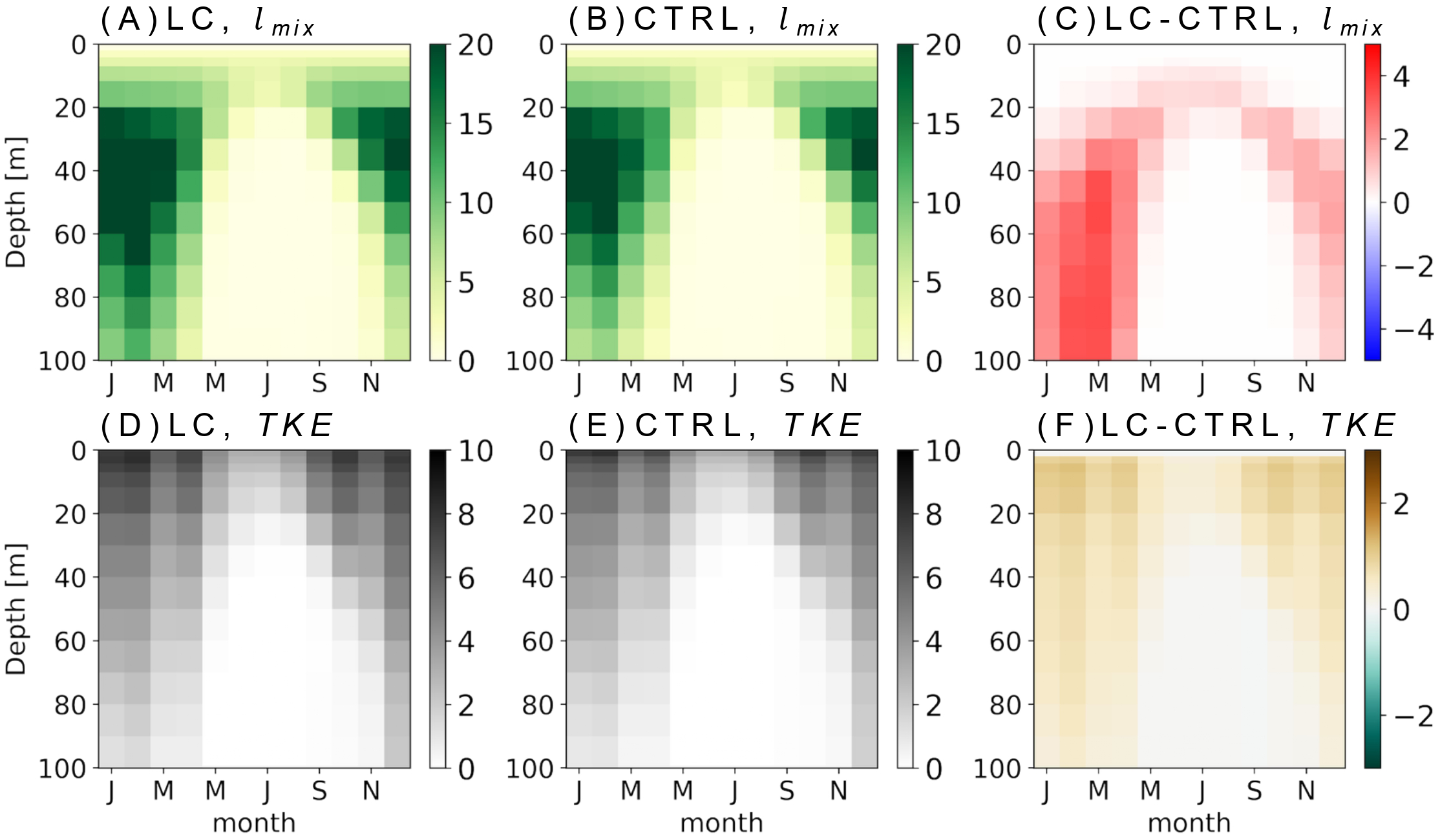
Seasonal cycle of vertical sections of (A–C)lmix (m) and (D–F) TKE (10−4 m2 s−2) in the Bering Sea basin.
To investigate the variability of air-sea carbon exchange due to the LC parameterization, we focus on changes. The exhibits a wintertime minimum and summertime maximum (Figure 3), with the simulated maximum occurring about 5 months later than the observation-based estimate (Supplementary Figure S2). This is a rather common discrepancy that many global biogeochemical models have in the North Pacific high latitudes (e.g., Carroll et al., 2020; Rodgers et al., 2023).
Figure 3
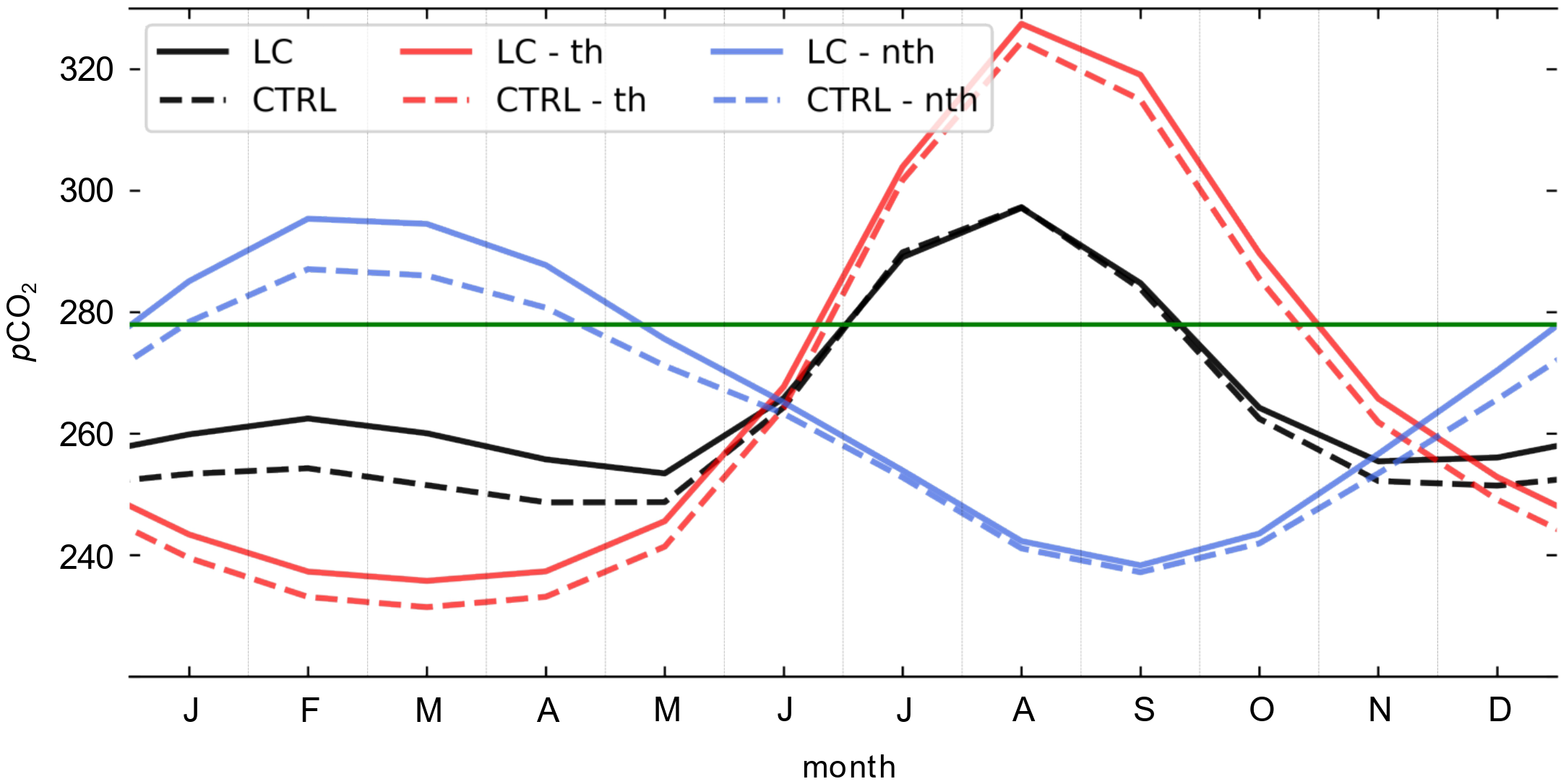
Seasonal cycle of pCO2 (black), its thermal component (, red), and non-thermal component ( blue) (µatm) averaged over the Bering Sea basin. The green horizontal line denotes the fixed atmospheric pCO2 (278 µatm).
To identify the cause of this mismatch, we decompose into thermal () and non-thermal () components using the approach of Takahashi et al. (2002).
In Equations 2 and 3, the overline indicates the spatiotemporal mean value over the Bering Sea basin region, and 0.0423 °C−1 is the sensitivity coefficient of pCO2 to SST (Takahashi et al., 1993). The accounts for the change induced by SST variations, and the is obtained by removing this SST effect from the total pCO2. The pCO2 decomposition reveals that the seasonal variability of is smaller than that of (Figure 3). This result contrasts with previous studies showing that in the Bering Sea, non-thermal effects play a dominant role over thermal effects in the seasonal variability of pCO2 (Song et al., 2016c; Zhang et al., 2023), which is consistent with the observation-based decomposition of pCO2 (Supplementary Figure S2). Consequently, the bias in seasonality largely accounts for the observed mismatch in total pCO2.
Focusing on the differences between the two experiments, the LC effect increases pCO2 and both of its components ( and ) during winter. In March, increases by 4.3 µatm due to the LC effect, which corresponds to approximately 13% of the seasonal standard deviation in CTRL . The LC effects on are minimal during summer, and this is consistent with the limited changes in vertical mixing, as indicated by little change in TKE and lmix (Figure 2). Overall, the LC effect slightly reduces the seasonal amplitude of by about 1% compared to CTRL, indicating that the thermal contribution is small.
The also contributes to a wintertime increase in pCO2. Among the factors that influence - namely DIC, salinity, and alkalinity - DIC has been identified as the primary driver of its seasonal variability in the Bering Sea (Gallego et al., 2018). In March, increases by 8.5 µatm, which is substantial given that its temporal standard deviation in the CTRL simulation is 17.12 µatm. As a result, the LC effect amplifies the seasonal amplitude of by 14% compared to CTRL.
The LC simulation exhibits that a large portion of the wintertime increase in pCO2 is explained by the . Typically, intensified vertical mixing leads and to offset each other (e.g., Mahadevan et al., 2004); however, our results show both components amplify the wintertime pCO2 increase. This atypical response is attributed to the Bering Sea’s vertical structure. In the following sections, we examine the vertical structure of temperature (thermal process) and DIC (non-thermal process), with particular focus on the winter season.
3.2 Vertical temperature profile
The Bering Sea is characterized by a temperature inversion (Miura et al., 2002, 2003; Ueno and Yasuda, 2005; Johnson and Stabeno, 2017). This inversion is well captured in the model simulations, which successfully reproduce the seasonal variation within the Bering Sea basin (Figures 4A, B). During winter, a temperature inversion emerges at the surface through surface cooling. In contrast, summertime surface heating suppresses temperature inversion near the surface, with the temperature inversion confined to the subsurface.
Figure 4
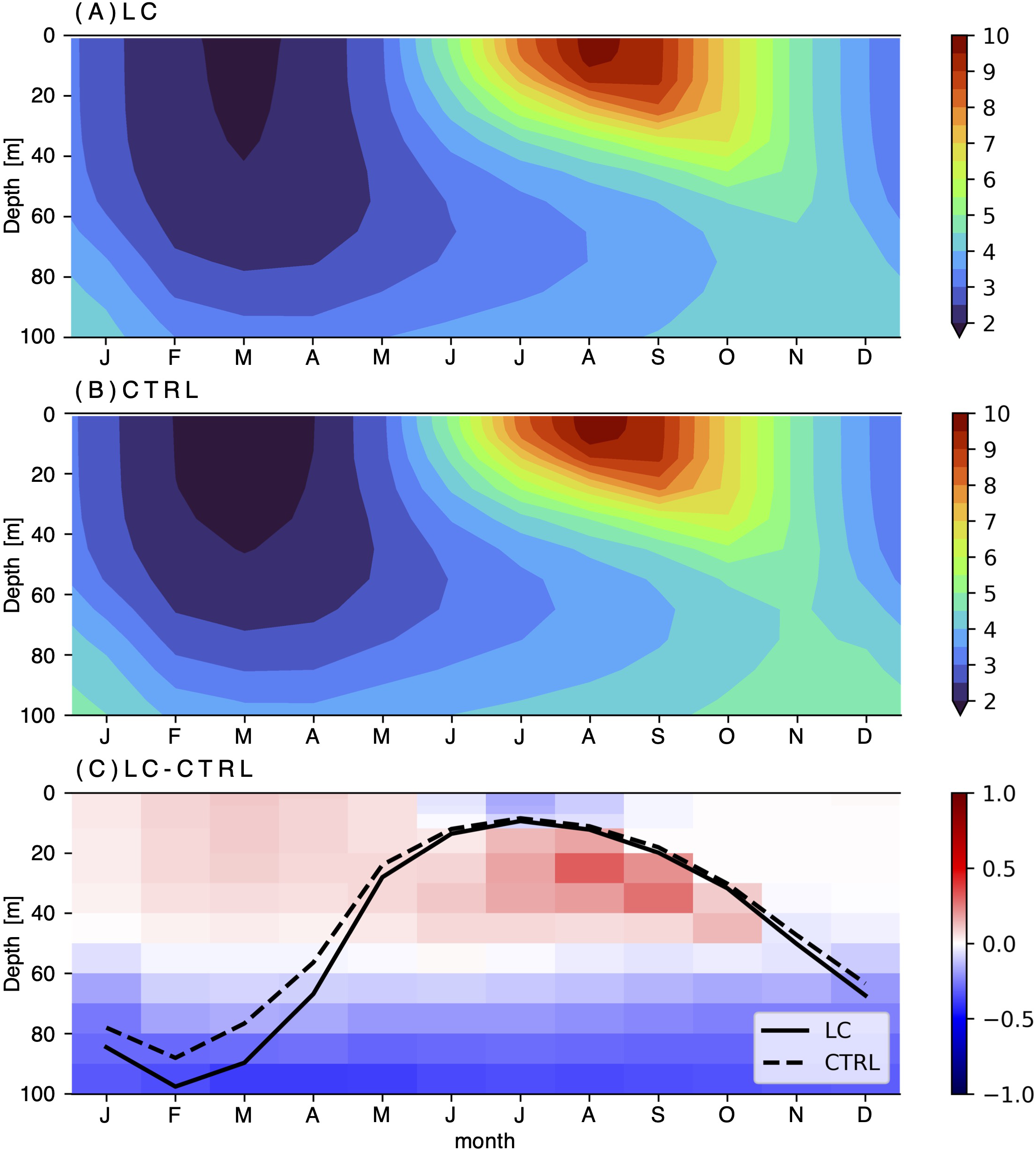
Seasonal cycle of vertical potential temperature (°C) profile for (A) LC, (B) CTRL and (C) LC minus CTRL in the Bering Sea basin. The black solid (dashed) line denotes the MLD of LC (CTRL).
Figure 4C illustrates the seasonal variation of the MLD along with the potential temperature difference between the two simulations. Enhanced vertical mixing deepens the MLD and warms the near-surface layer down to approximately 50 m, resulting in a 0.1°C increase in March SST relative to the CTRL simulation. This warming increases wintertime . If the Bering Sea had followed a thermally stratified structure within the reach of the LC effects, intensified winter mixing would decrease . Therefore, the temperature inversion in the Bering Sea plays a pivotal role in regulating .
3.3 Dissolved inorganic carbon
Vertical mixing alters the DIC vertical structure in the Bering Sea, where DIC concentration generally increases with depth (Dubinina et al., 2024; Chen et al., 2014; Keppler et al., 2020). In order to quantify the impact of LC on DIC concentration, we conducted a monthly DIC budget analysis for the Bering Sea. The tendency of DIC is written as
In Equation 4, ADVDIC represents the horizontal and vertical advection of DIC, MIXDIC denotes its horizontal and vertical diffusion (the vertical diffusion being more than three orders of magnitude larger than the horizontal diffusion), BIODIC accounts for biological sources and sinks via inorganic and organic processes, and represents the air–sea CO2 flux at the surface layer (0 to 2 m).
The DIC tendency has a seasonal variability within the MLD, increasing in winter and decreasing in summer in both experiments (Figures 5A, B), which is closely associated with the seasonal pattern of (Figure 3). Among the DIC budget, MIXDIC is the key driver of this seasonality within the MLD, showing a positive contribution during winter when intensified turbulent mixing promotes upward DIC entrainment (Figures 5B, E, H, K). ADVDIC also influences the DIC tendency, but its contribution is the opposite sign of MIXDIC within the MLD (Figures 5E, H). BIODIC contributes to reducing DIC during the spring; however, its overall influence remains limited compared to MIXDIC and ADVDIC (Figures 5E, H, K).
Figure 5
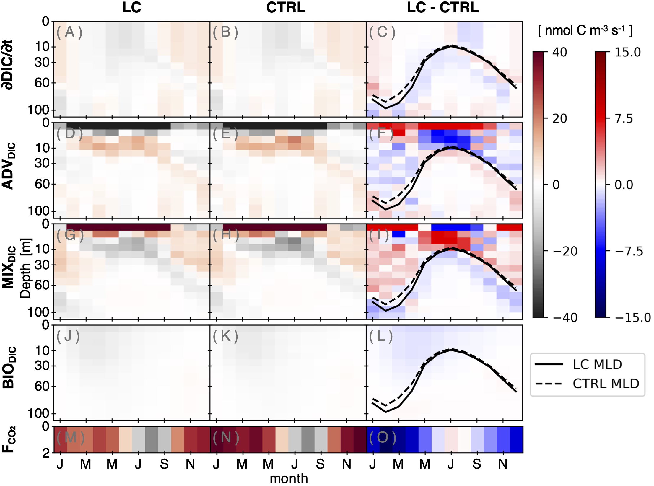
Seasonal cycle of vertical profile of DIC budget terms in the Bering Sea basin: (A–C) tendency of DIC, (D–F) advection of DIC, (G–I) diffusion of DIC, (J–L) biological source/sink, and (M–O) air-sea CO2 flux in the surface layer (0 to 2 m) (positive for oceanic uptake). The black solid (dashed) line denotes the MLD of LC (CTRL).
The surface DIC budget is primarily controlled by three terms— , MIXDIC, and ADVDIC (Figures 5E, H, N). Between February and September, a DIC increase induced by MIXDIC is largely compensated by ADVDIC (Figures 5E, H), with varying seasonally, exhibiting oceanic uptake during winter and outgassing during summer (Figure 5N), balancing the DIC changes driven by physical processes.
The comparison between the two experiments highlights the importance of wintertime MIXDIC (Figures 5C, F, I, L). In the LC simulation, increased vertical mixing during winter leads to intense upward entrainment from carbon-rich deep water to the surface. Consequently, the DIC supply through MIXDIC in the LC simulation exceeds that in the CTRL by approximately 0.03 GtC/year within the upper 100 m in February, whereas this difference becomes negligible (−0.0002 GtC/year) in August (Figure 5I). The wintertime increase is mitigated by ADVDIC and BIODIC (Figures 5F, L). ADVDIC dominates the wintertime reduction in DIC, whereas BIODIC contributes a relatively small decrease in spring.
At the surface layer, the LC parameterization increases both vertical mixing (MIXDIC) and advection (ADVDIC) of DIC during winter, deviating from the typical compensatory relationship between these two terms (Figures 5F, I). In response to LC, wintertime CO2 uptake decreases (Figure 5O), which helps to close the surface DIC budget. In the LC simulation, the surface ADVDIC, responsible for the wintertime reduction of DIC, is weakened (Figure 5F) due to reduced horizontal outflow from the basin (Supplementary Figure S3), contributing to the increase in pCO2. Therefore, the combination of enhanced supply through MIXDIC and weakened decrease through ADVDIC increases surface DIC, which reduces wintertime CO2 uptake in the LC simulation relative to the CTRL (Figures 5F, I, O). In contrast, differences between the two simulations are considerably smaller in summer than in winter (Figure 5O). The suppressed CO2 uptake persists except during summer, leading to a net decrease in annual CO2 uptake (Figure 5O).
The LC response on pCO2 in the Bering Sea exhibits a seasonal asymmetry. During winter, enhanced carbon supply elevates pCO2, which suppresses oceanic CO2 uptake. Increasing pCO2 is supported by surface warming, but its effect is minor compared to DIC entrainment. In contrast with the winter response, the summer response shows small differences between the two simulations, indicating the limited impact of LC during this period. Consequently, the LC effect is important in winter, when enhanced DIC entrainment associated with non-thermal processes dominates the air–sea CO2 exchange.
4 Summary and discussion
This study evaluates the impact of LC parameterization on vertical mixing and the carbon cycle in the Bering Sea basin using a physical–biogeochemical coupled ocean model. In the model experiments, LC is implemented to enhance turbulent mixing near the surface, and its impact is pronounced during winter. In this season, the Bering Sea can be characterized by a temperature inversion layer, with surface waters cooler than the underlying layers. Under such conditions, enhanced vertical mixing by LC raises SST, which in turn increases pCO2. Simultaneously, the deepened mixed layer driven by intensified turbulence facilitates the upward entrainment of carbon-rich subsurface water. As a result, surface ocean pCO2 increases during winter. This behavior contrasts with many other ocean regions, where enhanced vertical mixing typically cools the surface and reduces pCO2, partially offsetting the upward entrainment of carbon-rich water (Mahadevan et al., 2011).
To evaluate the contribution of LC to the carbon cycle and the seasonal variability of pCO2 in the Bering Sea, we decompose the LC-induced changes in pCO2 into thermal and non-thermal components. The LC effect slightly increases the thermal component of pCO2 throughout the year, resulting in a minor (1.4 µatm) reduction in its seasonal amplitude. A large portion of the wintertime pCO2 increase comes from the non-thermal component, which is associated with enhanced upward entrainment of DIC. Specifically, the non-thermal effect of LC amplifies the seasonal amplitude of pCO2 by 7.2 µatm. This increased seasonality brought by LC helps narrow the gap between the model results and observations.
In summary, parameterizing LC and applying it to a physical-biogeochemical coupled ocean model improves the seasonal variability of non-thermal effects. The existence of temperature inversion is vital for the clear expression of both thermal and non-thermal effects of LC. If a wintertime temperature inversion does not develop, LC leads to a decrease in SST, which offsets the non-thermal increase in pCO2. Thus, the wintertime temperature inversion prevents the suppression of the LC-induced non-thermal amplification of pCO2 in the Bering Sea basin.
In our study, both λ and Γ are prescribed as constant values, which is a reasonable assumption based on the previous studies. For example, Noh et al. (2016) showed that ocean general circulation model outputs are only weakly sensitive to the prescribed Γ and λ within typical observational ranges. When La is sufficiently small to ensure a large Γ, the LC-induced changes in MLD and SST remain largely unaffected by Γ variations, and the sensitivity to λ is also weak, with λ-induced MLD differences accounting for only about 6–7% of the difference between simulations with and without LC. Although the expected overall mean changes resulting from varied values for λ and Γ remain small, their cumulative biogeochemical influence over longer timescales may become non-negligible, necessitating further improvements in parameterization. Therefore, future work should investigate the potential effects of time-varying λ and Γ to better represent turbulent mixing processes and their associated biogeochemical responses, particularly those influencing the oceanic carbon cycle.
Statements
Data availability statement
The data analyzed in this study is subject to the following licenses/restrictions: The datasets for this study are available from the corresponding author upon reasonable request. Requests to access these datasets should be directed to HS, hajsong@yonsei.ac.kr.
Author contributions
KK: Conceptualization, Methodology, Visualization, Writing – original draft. HaS: Writing – review & editing, Funding acquisition, Methodology, Supervision, Writing – original draft. YC: Writing – review & editing. YT: Writing – review & editing, Methodology. JY: Writing – review & editing. HyS: Writing – review & editing. JL: Writing – review & editing.
Funding
The author(s) declared that financial support was received for this work and/or its publication. This research was supported by the Research Program for the carbon cycle between oceans, land, and atmosphere of the National Research Foundation (NRF) funded by the Ministry of Science and ICT (2022M3I6A1085990), and Korea Polar Research Institute (KOPRI) grant funded by the Ministry of Oceans and Fisheries (KOPRI, PE25110). HS also acknowledges the support from the Korea Meteorological Administration Research and Development Program under Grant RS-2025-02221669.
Acknowledgments
We would like to thank the reviewers for their comments, and we are especially grateful to Dr. Christopher Danek for the insightful feedback, which helped improve the paper.
Conflict of interest
The authors declared that this work was conducted in the absence of any commercial or financial relationships that could be construed as a potential conflict of interest.
Generative AI statement
The author(s) declare that Generative AI was used in the creation of this manuscript, especially for English editing to improve readability and grammar.
Any alternative text (alt text) provided alongside figures in this article has been generated by Frontiers with the support of artificial intelligence and reasonable efforts have been made to ensure accuracy, including review by the authors wherever possible. If you identify any issues, please contact us.
Publisher’s note
All claims expressed in this article are solely those of the authors and do not necessarily represent those of their affiliated organizations, or those of the publisher, the editors and the reviewers. Any product that may be evaluated in this article, or claim that may be made by its manufacturer, is not guaranteed or endorsed by the publisher.
Supplementary material
The Supplementary Material for this article can be found online at: https://www.frontiersin.org/articles/10.3389/fmars.2025.1684109/full#supplementary-material
References
1
Adcroft A. Hill C. Campin J.-M. Marshall J. Heimbach P. (2004). “ Overview of the formulation and numerics of the MIT GCM,” in Proceedings of the ECMWF Seminar Series on Numerical Methods, Recent Developments in Numerical Methods for Atmosphere and Ocean Model. 139–149 (ECMWF).
2
Adcroft A. Hill C. Marshall J. (1997). Representation of topography by shaved cells in a height coordinate ocean model. Monthly Weather Rev.125, 2293–2315. doi: 10.1175/1520-0493(1997)125<2293:ROTBSC>2.0.CO;2
3
Ahmed M. M. M. Else B. G. T. Capelle D. Miller L. A. Papakyriakou T. (2020). Underestimation of surface pCO2 and air-sea CO2 fluxes due to freshwater stratification in an Arctic shelf sea, Hudson bay. Elem. Sci. Anth. 8, 084. doi: 10.1525/elementa.084
4
Bates N. R. Mathis J. T. Jeffries M. A. (2011). Air-sea CO2 fluxes on the Bering Sea shelf. Biogeosciences8, 1237–1253. doi: 10.5194/bg-8-1237-2011
5
Belcher S. E. Grant A. L. M. Hanley K. E. Fox-Kemper B. Roekel L. V. Sullivan P. P. et al . (2012). A global perspective on Langmuir turbulence in the ocean surface boundary layer. Geophys. Res. Lett.39, L18605. doi: 10.1029/2012GL052932
6
Blanke B. Delecluse P. (1993). Variability of the tropical Atlantic Ocean simulated by a general circulation model with two different mixed-layer physics. J. Phys. Oceanography23, 1363–1388. doi: 10.1175/1520-0485(1993)023<1363:VOTTAO>2.0.CO;2
7
Carroll D. Menemenlis D. Adkins J. F. Bowman K. W. Brix H. Dutkiewicz S. et al . (2020). The ECCO-Darwin data-assimilative global ocean biogeochemistry model: Estimates of seasonal to multidecadal surface ocean pCO2 and air-sea CO2 flux. J. Adv. Modeling Earth Syst.12, e2019MS001888. doi: 10.1029/2019MS001888
8
Chen L. Gao Z. Sun H. Chen B. Cai W-j. (2014). Distributions and air-sea fluxes of CO2 in the summer Bering Sea. Acta Oceanol. Sin.33, 1–8. doi: 10.1007/s13131-014-0483-9
9
de Boyer Montégut C. (2023). Mixed layer depth climatology computed with a density threshold criterion of 0.03kg/m3 from 10 m depth value ( SEANOE). doi: 10.17882/91774
10
de Boyer Montégut C. Madec G. Fischer A. S. Lazar A. Iudicone D. (2004). Mixed layer depth over the global ocean: An examination of profile data and a profile-based climatology. J. Geophysical Res.: Oceans109, C12003. doi: 10.1029/2004JC002378
11
Dong Y. Yang M. Bakker D. C. E. Liss P. S. Kitidis V. Brown I. et al . (2021). Near-surface stratification due to ice melt biases arctic air-sea CO2 flux estimates. Geophys. Res. Lett.48, e2021GL095266. doi: 10.1029/2021GL095266
12
Dubinina E. O. Kossova S. A. Chizhova Y. N. Avdeenko A. S. (2024). Dissolved inorganic carbon (δ13C (DIC),[DIC]) in waters of the western Bering sea. Oceanology64, 681–694. doi: 10.1134/S000143702470036X
13
Dutkiewicz S. Sokolov A. Scott J. Stone P. (2005). “ A three-dimensional ocean-seaice-carbon cycle model and its coupling to a two-dimensional atmospheric model: uses in climate change studies,” in Joint Program on the Sci. Policy Global Change ( MIT, Cambridge, MA), Rep. 122.
14
Edwing K. Wu Z. Lu W. Li X. Cai W. Yan X. (2024). Impact of marine heatwaves on air-sea CO2 flux along the US East Coast. Geophysical Res. Lett.51, e2023GL105363. doi: 10.1029/2023GL105363
15
Fiechter J. Curchitser E. N. Edwards C. A. Chai F. Goebel N. L. Chavez F. P. (2014). Air-sea CO2 fluxes in the California current: Impacts of model resolution and coastal topography. Global Biogeochemical Cycles28, 371–385. doi: 10.1002/2013GB004683
16
Ford D. J. Tilstone G. H. Shutler J. D. Kitidis V. Sheen K. L. Dall’Olmo G. et al . (2023). Mesoscale eddies enhance the air-sea CO2 sink in the South Atlantic Ocean. Geophys. Res. Lett.50, e2022GL102137. doi: 10.1029/2022GL102137
17
Forget G. Campin J.-M. Heimbach P. Hill C. N. Ponte R. M. Wunsch C. (2015). ECCO version 4: an integrated framework for non-linear inverse modeling and global ocean state estimation. Geosci. Model. Dev.8, 3071–3104. doi: 10.5194/gmd-8-3071-2015
18
Gallego M. A. Timmermann A. Friedrich T. Zeebe R. E. (2018). Drivers of future seasonal cycle changes in oceanic pCO2. Biogeosciences15, 5315–5327. doi: 10.5194/bg-15-5315-2018
19
Gaspar P. Grégoris Y. Lefevre J. (1990). A simple eddy kinetic energy model for simulations of the oceanic vertical mixing: Tests at station papa and long-term upper ocean study site. J. Geophysical Res.: Oceans95, 16179–16193. doi: 10.1029/JC095iC09p16179
20
Guo Y. Timmermans M. (2024). The role of ocean mesoscale variability in air-sea CO2 exchange: A global perspective. Geophys. Res. Lett. 51, e2024GL108373. doi: 10.1029/2024GL108373
21
Hayden E. E. O’Neill L. W. (2024). Processes contributing to Bering Sea temperature variability in the late twentieth and early twenty-first century. J. Clim.37, 41–58. doi: 10.1175/JCLI-D-23-0331.1
22
Jersild A. Landschützer P. Gruber N. Bakker D. C. E. (2017). An observation-based monthly global gridded sea surface pCO2 and air-sea CO2 flux product from 1982 onward its monthly climatology ( NCEI Accession 0160558). National Oceanic and Atmospheric Administration). doi: 10.7289/v5z899n6
23
Johnson G. C. Stabeno P. J. (2017). Deep Bering Sea circulation and variability 2001–2016, from argo data. J. Geophysical Res.: Oceans122, 9765–9779. doi: 10.1002/2017JC013425
24
Keppler L. Landschützer P. Gruber N. Lauvset S. K. Stemmler I. (2020). Seasonal carbon dynamics in the near-global ocean. Global Biogeochemical Cycles34, e2020GB006571. doi: 10.1029/2020GB006571
25
Key R. M. Kozyr A. Sabine C. L. Lee K. Wanninkhof R. Bullister J. L. et al . (2004). A global ocean carbon climatology: Results from global data analysis project (GLODAP). Global Biogeochemical Cycles18, GB4031. doi: 10.1029/2004GB002247
26
Kim D. Lee S.-E. Cho S. Kang D.-J. Park G.-H. Kang S. K. (2022). Mesoscale eddy effects on sea-air CO2 fluxes in the northern philippine sea. Front. Mar. Sci.9. doi: 10.3389/fmars.2022.970678
27
Kwak K. Song H. Marshall J. Seo H. McGillicuddy D. J. (2021). Suppressed pCO2 in the Southern Ocean due to the interaction between current and wind. J. Geophysical Res.: Oceans126, e2021JC017884. doi: 10.1029/2021JC017884
28
Langmuir I. (1938). Surface motion of water induced by wind. Science87, 119–123. doi: 10.1126/science.87.2250.119
29
Large W. G. Yeager S. G. (2004). Diurnal to decadal global forcing for ocean and sea-ice models: The data sets and flux climatologies.
30
Lerner P. Romanou A. Kelley M. Romanski J. Ruedy R. Russell G. (2021). Drivers of air-sea CO2 flux seasonality and its long-term changes in the NASA-GISS Model CMIP6 submission. J. Adv. Modeling Earth Syst.13, e2019MS002028. doi: 10.1029/2019MS002028
31
Li Q. Webb A. Fox-Kemper B. Craig A. Danabasoglu G. Large W. G. et al . (2016). Langmuir mixing effects on global climate: WAVEWATCH III in CESM. Ocean Model.103, 145–160. doi: 10.1016/j.ocemod.2015.07.020
32
Luo C. Mahowald N. Bond T. Chuang P. Y. Artaxo P. Siefert R. et al . (2008). Combustion iron distribution and deposition. Global Biogeochemical Cycles22, GB1012. doi: 10.1029/2007GB002964
33
Mahadevan A. Lévy M. Mémery L. (2004). Mesoscale variability of sea surface pCO2: What does it respond to? Global Biogeochemical Cycles18, GB1017. doi: 10.1029/2003GB002102
34
Mahadevan A. Tagliabue A. Bopp L. Lenton A. Mémery L. Lévy M. (2011). Impact of episodic vertical fluxes on sea surface pCO2. Philos. Trans. R. Soc A Math. Phys. Eng. Sci.369, 2009–2025. doi: 10.1098/RSTA.2010.0340
35
Marshall J. Adcroft A. Hill C. Perelman L. Heisey C. (1997a). A finite-volume, incompressible Navier Stokes model for studies of the ocean on parallel computers. J. Geophys. Res.102, 5753–5766. doi: 10.1029/96JC02775
36
Marshall J. Hill C. Perelman L. Adcroft A. (1997b). Hydrostatic, quasi-hydrostatic, and nonhydrostatic ocean modeling. J. Geophys. Res.102, 5733–5752. doi: 10.1029/96JC02776
37
Marshall J. Jones H. Hill C. (1998). Efficient ocean modeling using non-hydrostatic algorithms. J. Mar. Sci.18, 115–134. doi: 10.1016/S0924-7963(98)00008-6
38
McKinley G. A. Takahashi T. Buitenhuis E. Chai F. Christian J. R. Doney S. C. et al . (2006). North Pacific carbon cycle response to climate variability on seasonal to decadal timescales. J. Geophysical Res.: Oceans111, C07S06. doi: 10.1029/2005JC003173
39
McWilliams J. C. Sullivan P. P. (2000). Vertical mixing by Langmuir circulations. Spill Sci.6, 225–237. doi: 10.1016/S1353-2561(01)00041-X
40
McWilliams J. C. Sullivan P. P. Moeng C.-H. (1997). Langmuir turbulence in the ocean. J. Fluid Mech.334, 1–30. doi: 10.1017/S0022112096004375
41
Miura T. Suga T. Hanawa K. (2002). Winter mixed layer and formation of dichothermal water in the Bering Sea. J. Oceanogr.58, 815–823. doi: 10.1023/A:1022871112946
42
Miura T. Suga T. Hanawa K. (2003). Numerical study of formation of dichothermal water in the bering sea. J. Oceanogr.59, 369–376. doi: 10.1023/A:1025524228857
43
Noh Y. Goh G. Raasch S. (2011). Influence of Langmuir circulation on the deepening of the wind-mixed layer. J. Phys. Oceanography41, 472–484. doi: 10.1175/2010JPO4494.1
44
Noh Y. Min H. S. Raasch S. (2004). Large eddy simulation of the ocean mixed layer: The effects of wave breaking and Langmuir circulation. J. Phys. Oceanography34, 720–735. doi: 10.1175/1520-0485(2004)034<0720:LESOTO>2.0.CO;2
45
Noh Y. Ok H. Lee E. Toyoda T. Hirose N. (2016). Parameterization of Langmuir circulation in the ocean mixed layer model using LES and its application to the OGCM. J. Phys. Oceanography46, 7–78. doi: 10.1175/JPO-D-14-0137.1
46
Parekh P. Follows M. J. Boyle E. A. (2005). Decoupling of iron and phosphate in the global ocean. Global Biogeochemical Cycles19, GB2020. doi: 10.1029/2004GB002280
47
Reichl B. G. Li Q. (2019). A parameterization with a constrained potential energy conversion rate of vertical mixing due to Langmuir turbulence. J. Phys. Oceanography49, 2935–2959. doi: 10.1175/JPO-D-18-0258.1
48
Reichl B. G. Wang D. Hara T. Ginis I. Kukulka T. (2016). Langmuir turbulence parameterization in tropical cyclone conditions. J. Phys. Oceanography46, 863–886. doi: 10.1175/JPO-D-15-0106.1
49
Rodgers K. B. Schwinger J. Fassbender A. J. Landschützer P. Yamaguchi R. Frenzel H. et al . (2023). Seasonal variability of the surface ocean carbon cycle: A synthesis. Global Biogeochemical Cycles37, e2023GB007798. doi: 10.1029/2023GB007798
50
Shevchenko G. V. Tshay Z. R. Lozhkin D. M. (2024). Spatiotemporal variability of Bering Sea surface temperature from satellite-based ERA5 reanalysis data. Izvestiya Atmos. Ocean. Phys.60, 1075–1085. doi: 10.1134/S0001433824701032
51
Shiomoto A. Saitoh S. Imai K. Toratani M. Ishida Y. Sasaoka K. (2002). Interannual variation in phytoplankton biomass in the Bering Sea basin in the 1990s. Prog. Oceanog.55, 147–163. doi: 10.1016/S0079-6611(02)00075-7
52
Smith K. M. Hamlington P. E. Niemeyer K. E. Fox-Kemper B. Lovenduski N. S. (2018). Effects of Langmuir turbulence on upper ocean carbonate chemistry. J. Adv. Modeling Earth Syst.10, 3030–3048. doi: 10.1029/2018MS001486
53
Smyth W. D. Skyllingstad E. D. Crawford G. B. Wijesekera H. (2002). Nonlocal fluxes and stokes drift effects in the K-profile parameterization. Ocean Dynamics52, 104–115. doi: 10.1007/s10236-002-0012-9
54
Song X. Bai Y. Cai W.-J. Chen C.-T. Pan D. He X. et al . (2016c). Remote sensing of sea surface pCO2 in the Bering Sea in summer based on a mechanistic semi-analytical algorithm (MeSAA). Remote Sens.8, 558. doi: 10.3390/rs8070558
55
Song H. Marshall J. Campin J. McGillicuddy D. J. (2019). Impact of near-inertial waves on vertical mixing and air-sea CO2 fluxes in the Southern Ocean. J. Geophysical Res.: Oceans124, 4605–4617. doi: 10.1029/2018JC014928
56
Song H. Marshall J. Follows M. J. Dutkiewicz S. Forget G. (2016a). Source waters for the highly productive Patagonian shelf in the southwestern Atlantic. J. Mar. Sci.158, 120–128. doi: 10.1016/j.jmarsys.2016.02.009
57
Song H. Marshall J. Munro D. R. Dutkiewicz S. Sweeney C. McGillicuddy D. J. et al . (2016b). Mesoscale modulation of air-sea CO2 flux in Drake Passage. J. Geophysical Res.: Oceans121, 6635–6649. doi: 10.1002/2016JC011714
58
Springer A. M. McRoy C. P. Flint M. V. (1996). The Bering Sea green belt: shelf-edge processes and ecosystem production. Fisheries Oceanography5, 205–223. doi: 10.1111/j.1365-2419.1996.tb00118.x
59
Tak Y.-J. Song H. Noh Y. Choi Y. (2023). Physical and biogeochemical responses in the Southern Ocean to a simple parameterization of Langmuir circulation. Ocean Model.181, 102152. doi: 10.1016/j.ocemod.2022.102152
60
Takahashi T. Olafsson J. Goddard J. G. Chipman D. W. Sutherland S. C. (1993). Seasonal variation of CO2 and nutrients in the high-latitude surface oceans: A comparative study. Global Biogeochemical Cycles7, 843–878. doi: 10.1029/93GB02263
61
Takahashi T. Sutherland S. C. Sweeney C. Poisson A. Metzl N. Tilbrook B. et al . (2002). Global sea–air CO2 flux based on climatological surface ocean pCO2, and seasonal biological and temperature effects. Deep Sea Res. Part II Top. Stud. Oceanogr., 49, 1601–1622. doi: 10.1016/S0967-0645(02)00003-6
62
Thorpe S. (2004). Langmuir circulation. Annu. Rev. Fluid Mech.36, 55–79. doi: 10.1146/annurev.fluid.36.052203.071431
63
Tyrrell T. Merico A. Waniek J. J. Wong C. S. Metzl N. Whitney F. (2005). Effect of seafloor depth on phytoplankton blooms in high-nitrate, low-chlorophyll (HNLC) regions. J. Geophysical Res.: Biogeosciences110, G02007. doi: 10.1029/2005JG000041
64
Ueno H. Yasuda I. (2005). Temperature inversions in the subarctic north Pacific. J. Phys. Oceanography35, 2444–2456. doi: 10.1175/JPO2829.1
65
Zhang S. Bai Y. He X. Jiang Z. Li T. Gong F. et al . (2023). Spatial and temporal variations in sea surface pCO2 and air-sea flux of CO2 in the Bering Sea revealed by satellite-based data during 2003–2019. Front. Mar. Sci.10. doi: 10.3389/fmars.2023.1099916
Summary
Keywords
Bering Sea, partial pressure of CO2, seasonality, temperature inversion, vertical mixing
Citation
Kwak K, Song H, Choi Y, Tak Y-J, Yun J, Seunu H and Lee J (2025) Effects of Langmuir circulation parameterization on seasonal air–sea CO2 exchange in the Bering Sea. Front. Mar. Sci. 12:1684109. doi: 10.3389/fmars.2025.1684109
Received
12 August 2025
Revised
28 November 2025
Accepted
28 November 2025
Published
15 December 2025
Volume
12 - 2025
Edited by
Youyu Lu, Bedford Institute of Oceanography (BIO), Canada
Reviewed by
Tien Anh Tran, Seoul National University, Republic of Korea
Christopher Danek, Alfred Wegener Institute Helmholtz Centre for Polar and Marine Research (AWI), Germany
Updates
Copyright
© 2025 Kwak, Song, Choi, Tak, Yun, Seunu and Lee.
This is an open-access article distributed under the terms of the Creative Commons Attribution License (CC BY). The use, distribution or reproduction in other forums is permitted, provided the original author(s) and the copyright owner(s) are credited and that the original publication in this journal is cited, in accordance with accepted academic practice. No use, distribution or reproduction is permitted which does not comply with these terms.
*Correspondence: Hajoon Song, hajsong@yonsei.ac.kr
Disclaimer
All claims expressed in this article are solely those of the authors and do not necessarily represent those of their affiliated organizations, or those of the publisher, the editors and the reviewers. Any product that may be evaluated in this article or claim that may be made by its manufacturer is not guaranteed or endorsed by the publisher.