Frequency adaptability analysis of typical acoustic propagation models

Underwater acoustic propagation is influenced by water column properties, seabed topography, and source frequency, with existing numerical models exhibiting varied performance across different conditions. This study evaluates the frequency adaptability of three acoustic models—BELLHOP (geometric ray-based), RAM (parabolic equation), and KRAKEN (coupled mode)—under diverse seabed topographies, including deep-sea-flat (25–2000 Hz), shallow-sea-flat (25–10000 Hz), and gentle/steep-slope seabed (25–800 Hz). Flat seabed scenarios use the Scooter model as a benchmark, while sloping seabed scenarios are compared against analytical solutions. Results indicate that in a 200 m deep flat ocean environment, BELLHOP achieves high accuracy for frequencies above 200 Hz, KRAKEN performs comparably to RAM below 50 Hz, and RAM excels below 200 Hz. In a 4000 m deep flat ocean, RAM outperforms at frequencies below 100 Hz, while BELLHOP performs well above 100 Hz. For sloping seabed environments with slopes less than 6.5°, RAM demonstrates stability below 100 Hz, while BELLHOP performs better above 100 Hz; for slopes greater than 6.5°, RAM remains stable below 50 Hz, with BELLHOP outperforming above 50 Hz. KRAKEN is found unsuitable for sloping seabed simulations. These findings provide quantitative guidance for selecting acoustic models based on frequency and seabed topography.

1 Introduction

Underwater sound propagation is fundamental to scientific research and engineering applications, such as underwater detection and communication. However, its characteristics are significantly influenced by factors including sound speed profiles (Li et al., 2022; Wu et al., 2022), seabed topography (Chen et al., 2022; Chai et al., 2022; King et al., 2023), and source frequency (Possenti et al., 2024). Numerical models of sound propagation, as primary tools for studying underwater acoustic characteristics, exhibit varying performance depending on specific topographic and frequency conditions.

Extensive prior research has explored the effects of frequency and topography on underwater sound propagation, providing critical insights into its behavior. Nevertheless, the impact of complex topography and frequency variations on model performance remains underexplored. Oliveira et al. (2021) compared three models—PE (parabolic equation), KRAKEN (normal mode), and BELLHOP (ray tracing)—in the complex shallow-water environment of Long Island Sound, analyzing topographic influences. Their findings indicate that in shoal terrains, the PE model outperforms KRAKEN and BELLHOP due to its ability to handle three-dimensional effects. In sloped terrains, KRAKEN exhibits steep root mean square error (RMSE) due to neglecting mode coupling, while PE remains more stable. In flat or mildly varying terrains, all three models perform similarly at short ranges, but PE and KRAKEN are more accurate at longer ranges. Dahl and Dall'Osto (2017) investigated underwater sound fields during offshore wind farm pile driving, comparing ray-tracing and PE models across frequencies. They found that ray-tracing models accurately capture arrival structures in high-frequency near-field scenarios, whereas PE models are more stable in far-field and low-frequency conditions. Ying-Tsong Lin et al. (Lin and Duda, 2012) developed an improved PE model and compared it with traditional PE models, demonstrating enhanced stability in range-dependent environments and low-frequency conditions. Ballard et al. (2015) analyzed 3D sound propagation over gentle-slope cosine-shaped hills, comparing normal-mode, PE, and BELLHOP models. Their results suggest that normal-mode models are suitable for gentle slopes but incur steep root mean square error (RMSE) at steeper slopes, PE excels in handling 3D effects, and BELLHOP performs well at high frequencies but struggles at low frequencies.

Despite these advances, current model applicability is often based on qualitative conclusions, lacking clear quantitative boundaries. For instance, BELLHOP is deemed suitable for high-frequency simulations, KRAKEN for low frequencies, and RAM for mid-to-low frequencies, yet specific frequency thresholds remain undefined. This study systematically evaluates the frequency adaptability of three acoustic models—BELLHOP, RAM, and KRAKEN—across diverse underwater environments. We analyze their performance in flat deep-sea seabed (25–2000 Hz), flat shallow-sea seabed (25–10000 Hz), and sloped seabed with gentle and large gradients (25–800 Hz). For sloped conditions, we adopt the analytical solution provided by G. B. Deane (Deane and Tindle, 1992), previously validated for accuracy, as the benchmark. For flat terrains, the Scooter wavenumber model serves as the reference. Through comprehensive comparisons, this study provides quantitative guidance for selecting optimal acoustic models based on specific frequency ranges and seabed topographies, addressing gaps in understanding model performance under combined frequency and topographic conditions.

2 Model descriptions

2.1 BELLHOP (ray-tracing model)

BELLHOP is a ray-tracing-based acoustic propagation model developed by Porter and Bucker (1987) for predicting sound pressure fields in range-dependent environments. The model employs ray-tracing techniques, with its core theory grounded in geometric acoustics. It computes sound wave propagation by solving ray path equations, supporting complex sound speed profiles and seabed topography variations. The sound pressure p(r, z) is expressed as the sum of contributions from individual ray paths, as shown in Equation 1:

$\begin{array}{ll}p(r,\text{z})={\displaystyle \sum _n{A}_n}{e}^{i{\phi }_n}& (1)\end{array}$

Where $A_n$ is the amplitude of the n-th ray, ${\phi }_n=k{s}_n$ is the phase, and $s_n$ is the path length. The wavenumber is denoted by $k=\frac{\omega }{c}$. BELLHOP, based on ray theory, is well-suited for deep-sea and high-frequency scenarios. However, in low-frequency shallow-water environments, its accuracy may be reduced due to the neglect of modal interference and diffraction effects (Jensen et al., 2011).

2.2 KRAKEN (normal-mode model)

KRAKEN is a normal mode-based acoustic propagation model developed by Michael B. Porter (1992), with its core principle centered on decomposing the sound field into depth-dependent mode functions and horizontal propagation factors. KRAKEN exhibits high computational efficiency at low frequencies, but its computational complexity increases significantly at high frequencies due to the rising number of modes. It is particularly well-suited for low-frequency shallow-water environments. Under the adiabatic approximation, KRAKEN is especially effective in weak range-dependent environments, where modal coupling effects can be neglected when seabed slopes are sufficiently gentle, yielding efficient and accurate simulation results. However, in environments with steeper slopes, neglecting modal coupling may compromise accuracy (Jensen et al., 2011). The sound pressure p(r, z) is expressed as the sum of modal contributions, as shown in Equation 2:

$\begin{array}{ll}p(r,z)={\displaystyle \sum _{m=1}^M{A}_m(r){\varphi }_m}(z)& (2)\end{array}$

Here, $A_m(r)$ represents the amplitude of the m-th mode, varying with range r, and ${\varphi }_m(z)$ is the modal function in range-independent environments, with M being the total number of modes. KRAKEN employs an efficient eigenvalue solver algorithm to overcome numerical instabilities inherent in traditional normal-mode models. It supports complex sound speed profiles and elastic seabed modeling, delivering robust performance in both shallow- and deep-water environments (Jensen et al., 2011).

2.3 RAM

RAM (Range-dependent Acoustic Model), developed by Michael D. Collins (1993), is an ocean acoustic propagation model based on the parabolic equation (PE) approach, designed for sound field calculations in range-dependent environments. It is well-suited for scenarios where topography and sound speed profiles vary with horizontal distance. RAM offers high computational efficiency and effectively handles range-dependent conditions, though finer grids are required at high frequencies to maintain accuracy. Additionally, RAM neglects backscattering effects, which may introduce root mean square error (RMSE) in strongly range-dependent environments. The model solves the parabolic equation to progressively advance the sound field along the horizontal range, supporting complex sound speed profiles and topographic variations. The sound field ψ(r, z) satisfies the governing equation, as shown in Equation 3:

$\begin{array}{ll}\frac{\partial \psi (r,z)}{\partial r}=i{k}_0(\sqrt{1+\frac{1}{k_0^2}(\frac{{\partial }^2}{\partial z^2}+k^2(z)-k_0^2)}-1)\psi (r,z)& (3)\end{array}$

Here $\psi (r,z)$ represents the sound field function, related to the sound pressure $p(r,z)$, and $k_0=\frac{\omega }{c_0}$denotes the reference wavenumber. Here, $\omega$ is the angular frequency, $c_0$ the reference sound speed, and $k(z)=\frac{\omega }{c(z)}$ the wavenumber, which varies with depth z, where c(z) is the sound speed varying with depth. The term $\frac{{\partial }^2}{\partial z^2}$ represents the second-order derivative in the depth direction, describing the variation of the sound field with depth. The final sound pressure is given by $p(r,z)=\psi (r,z)\frac{e^{i{k}_{0}r}}{\sqrt{r}}$. RAM is well-suited for broadband scenarios, offering high computational efficiency, and is widely applied in sonar design and shallow-water acoustic research (Jensen et al., 2011).

2.4 SCOOTER (fast field program model)

SCOOTER, developed by Fredrick D. Tappert and Michael B. Porter (Porter and Bucker, 1987), is an ocean acoustic propagation model based on the Fast Field Program (FFP) approach, designed for sound field calculations in range-independent environments (Li et al., 2022). Its core method leverages the Fast Fourier Transform (FFT) to compute the sound field distribution by transforming between the wavenumber and spatial domains. The model first solves the depth-separated Helmholtz equation to obtain the Green’s function $G(k_r,z,z_s)$ followed by FFT-based computation of the sound pressure $p(r,z)$. This approach essentially provides a fast implementation of wavenumber integration without direct numerical quadrature, resulting in high computational efficiency. SCOOTER offers high accuracy and is well-suited for low- to mid-frequency scenarios in range-independent environments, where it neglects backscattering effects. The sound pressure p(r, z) is represented as the solution to the governing equation, as shown in Equation 4:

$\begin{array}{ll}p(r,z)=FF{T}^{-1}[G(k_r,z,z_s)H(k_r,r)]& (4)\end{array}$

Here, $G(k_r,z,z_s)$ denotes the Green’s function, representing the depth-dependent sound field response corresponding to the wavenumber $k_r$, $H(k_r,r)$ is the horizontal propagation factor, and $k_r$ is the horizontal wavenumber. SCOOTER employs a finite difference method to solve for the Green’s function. The model achieves high accuracy in flat seabed calculations, making it suitable as a benchmark solution for flat ocean conditions.

2.5 Mirror solution model

Deane and Tindle (1992) proposed an analytical model for sound propagation in three-dimensional wedge-shaped environments, applicable to ocean settings with constant sound speed profiles and penetrable bottoms. Based on the source-image method, the model represents the total sound field as a linear superposition of contributions from multiple source images, each corresponding to successive reflections of sound waves at the wedge boundaries. By employing plane wave expansion and the method of steepest descent, the model performs asymptotic analysis of the sound field integral to derive analytical solutions for the sound field. The total sound field is expressed as the sum of these contributions, as shown in Equation 5:

$\begin{array}{ll}P(R_w)={\displaystyle \sum _{n_b=0}^{n_{\max }}{\displaystyle \sum _l{p}_{nl}(R)}}& (5)\end{array}$

Here, $p_{nl}(R)$, is computed for the source image $S_{nl}$ using Fourier transforms and reflection coefficients. The model specifically accounts for three-dimensional effects by introducing a loss factor ∈ to describe the impact of reflections. By employing plane wave expansion and the method of steepest descent, the model performs asymptotic analysis of the sound field integral to derive analytical solutions for the sound field. This approach is suitable for range-dependent environments, enabling accurate prediction of the sound field in wedge-shaped cross-sections, with results consistent with those of the narrow-angle parabolic equation and coupled-mode methods, achieving errors within 1 dB (Lin and Duda, 2012). The model serves as a benchmark solution for upslope conditions.

The main mathematical symbols and notations used throughout this study are summarized in Table 1.

Table 1

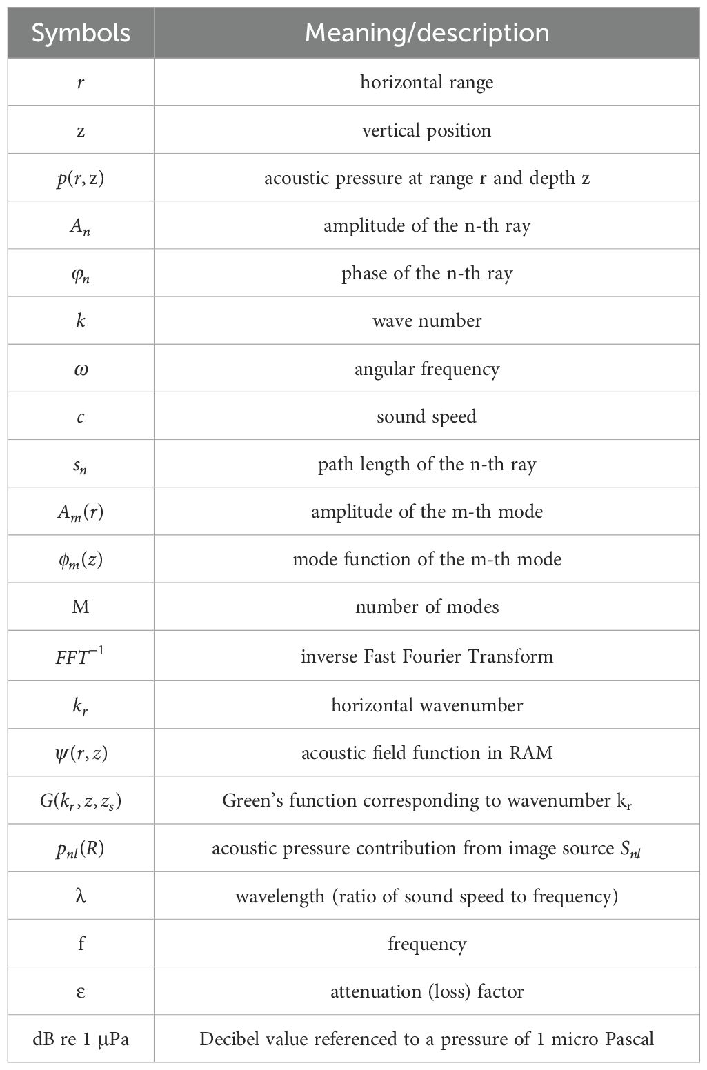
Table 1. Notation table.

3 Simulation and analysis under flat conditions

3.1 Simulation under shallow-sea flat conditions

Shallow-water flat environments typically refer to ocean regions with water depths less than 200 m and minimal seabed undulations. In such environments, sound propagation is significantly influenced by the sea surface and seabed boundaries. During propagation, sound waves undergo multiple reflections between the seabed and sea surface, leading to rapid attenuation. Additionally, high-frequency sound waves experience substantial losses due to absorption and scattering, limiting their propagation range.

To evaluate the performance of various simulation models across different frequency bands in shallow-water flat conditions, we standardized the basic Parameters of all models, including range intervals and horizontal spacing, to ensure computational accuracy. The simulation setup was configured with a seabed depth of 200 m and a range of 0–10 km. The sound speed profile was assumed to be constant, as depicted in Figure 1. The seabed was modeled with a common fine sand sediment type, characterized by a sound speed of 1700 m/s, a density of 1500kg/m³, and an attenuation of 0.5 dB/λ. This fine sand seabed property was consistently applied in all subsequent simulations. For the simulations, frequencies of 25, 50, 100, 200, 500, 700, 1k, 2k, 5k, and 10kHz were selected. The sound source was placed at a depth of 100 m, and the transmission loss was calculated at a receiver depth of 30 m. Results were compared with the SCOOTER model, with comparison outcomes shown in Figure 2 and statistical root mean square error (RMSE) for 4 km and 10 km ranges presented in Figure 3; Tables 2, 3. In this study, all transmission loss (TL), and RMSE values are expressed in decibels (dB) relative to a reference pressure of 1 μPa (i.e., dB re 1 μPa).

Figure 1

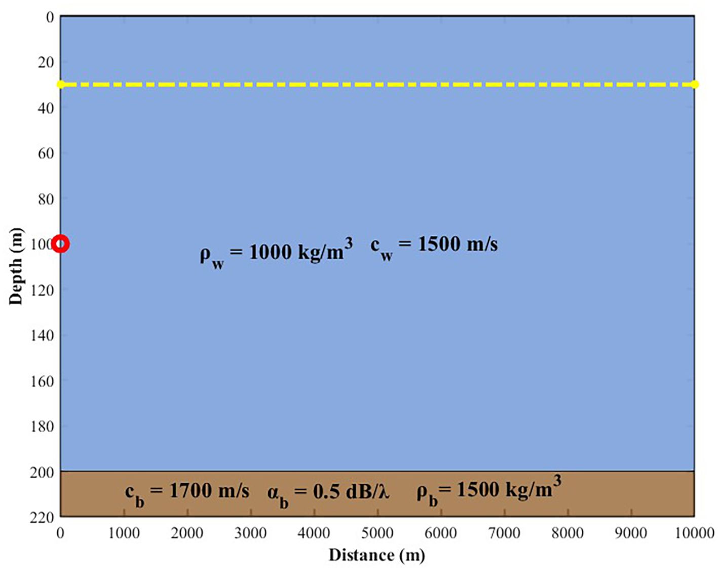
Figure 1. Topography and sound speed profile used in shallow-sea simulations. The red dot indicates the sound source position, and the yellow lines indicates the receiver position.

Figure 2

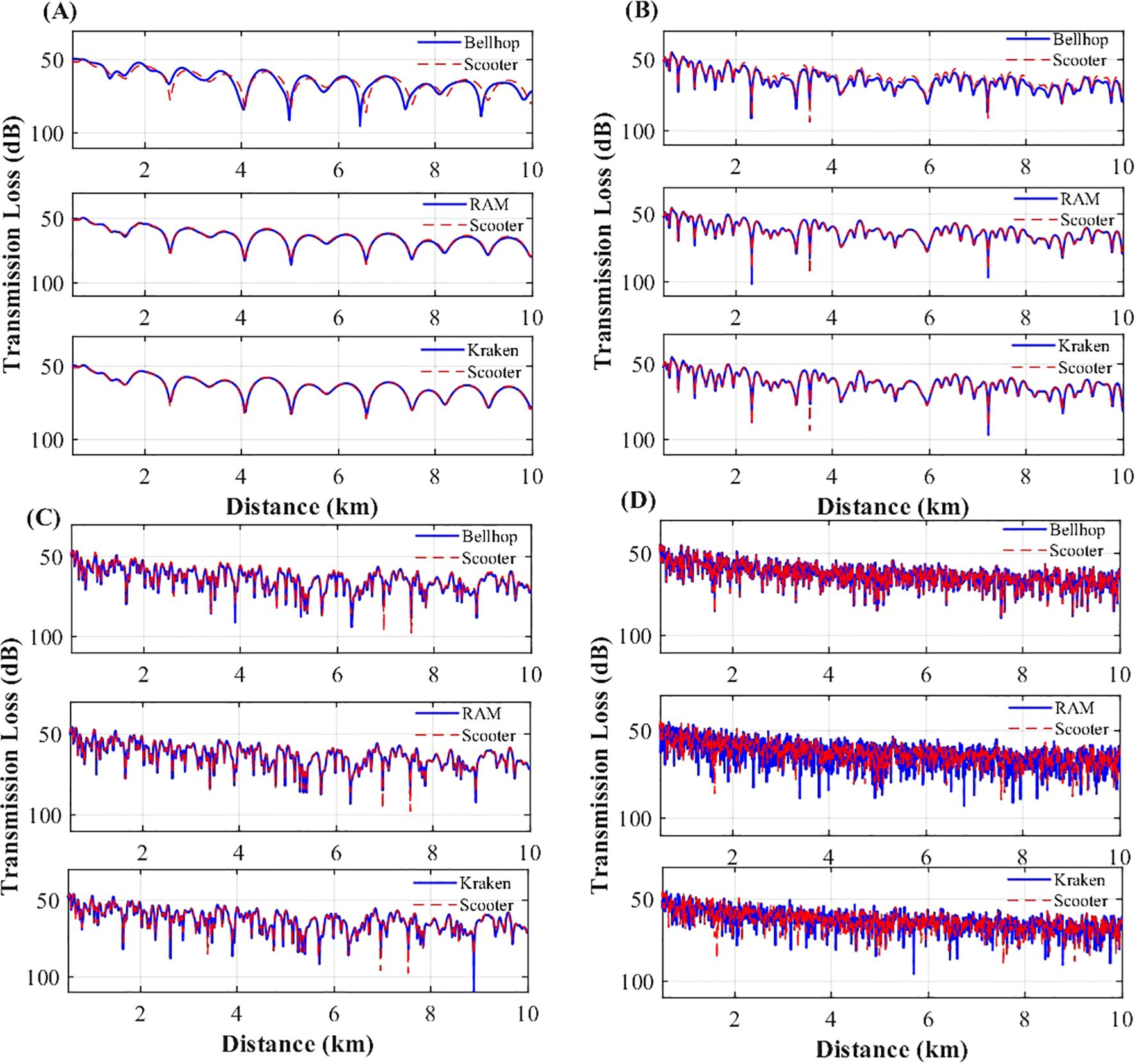
Figure 2. Transmission loss comparison for shallow-sea simulations over a 10 km range. (A) Comparison results at 25 Hz, (B) Comparison results at 100 Hz, (C) Comparison results at 200 Hz, (D) Comparison results at 2000 Hz.

Figure 3

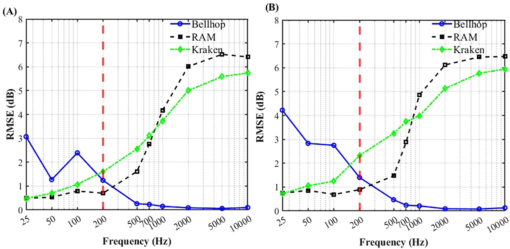
Figure 3. Comparison of root mean square error (RMSE) in the shallow-sea environment. The red dashed line indicates the frequency threshold separating the low-frequency (RAM-dominant) and high-frequency (BELLHOP-dominant) regions (A) Propagation range of 4 km; (B) Propagation range of 10 km.

Table 2

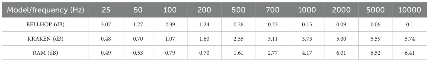
Table 2. Statistical root mean square error (RMSE) results for shallow-sea simulations over a 4km range.

Table 3

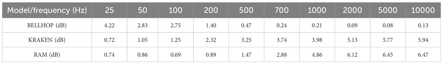
Table 3. Statistical root mean square error (RMSE) results for shallow-sea simulations over a 10km range.

Through comparative analysis under shallow-sea flat conditions, performance variations due to distance and frequency are evident. In short-range (4 km) simulations, RAM achieves the highest accuracy for frequencies below 200 Hz, followed by KRAKEN, while BELLHOP performs the least effectively. particularly at 25 Hz, where RAM and KRAKEN result closely match the benchmark solution, whereas BELLHOP shows significant deviation beyond 2.5 km.

For frequencies above 200 Hz, BELLHOP exhibits optimal simulation accuracy, confirming its high precision in high-frequency regimes. Additionally, RAM outperforms KRAKEN in the 200–700 Hz range but is less accurate than BELLHOP, aligning with the theoretical foundations of each model. In 10 km range simulations, BELLHOP’s RMSE at 25 Hz increases significantly compared to the 4 km results.

In summary, BELLHOP, based on ray theory, is suitable for 200 Hz–10 kHz short-wavelength scenarios and excels in short-range propagation. KRAKEN is appropriate for shallow-water waveguide environments below 50 Hz. RAM, based on the parabolic equation, is optimal for 0–200 Hz frequencies and long-range simulations.

3.2 Simulation under deep-sea flat conditions

Deep-sea environments generally refer to ocean regions with water depths exceeding 1000 m. Compared to shallow-water environments, sound propagation in deep seas is less influenced by boundary effects. In shallow water, sound wave propagation is dominated by reflected waves; however, in deep-sea conditions, direct waves play a predominant role. After reflection from the deep-sea seabed, sound energy attenuates sharply. Furthermore, deep-sea propagation is significantly affected by the sound speed profile. For instance, sound traveling along the sound channel axis can achieve long-range propagation.

To evaluate the performance of various models across different frequency bands in deep-sea propagation, we adopted a typical Munk sound speed profile for the deep-sea analysis. The ocean depth was set to 4000 m, with the sound speed profile and topography depicted in Figure 4. The sound source was positioned at a depth of 300 m, and the transmission loss received at a depth of 350 m was analyzed and compared. For root mean square error (RMSE) analysis, this study selected the range of 20–70 km for root mean square error (RMSE) calculations, based on the following considerations: firstly, the near-field sound field within 0–20 km is complex, and root mean square error (RMSE) in this range may be influenced by interference and environmental modeling uncertainties, reflecting more on the limitations of environmental modeling rather than the simulation capabilities of the models; secondly, environmental parameters in the 20–70 km range are relatively stable, making root mean square error (RMSE) analysis more targeted. The transmission loss comparison results of different models with the SCOOTER benchmark are shown in Figure 5, with RMSE statistics presented in Table 4; Figure 6.

Figure 4

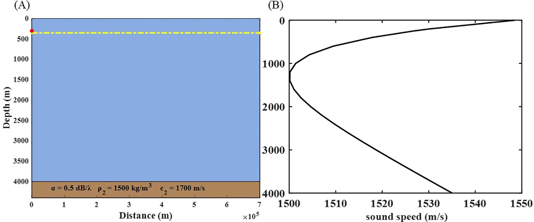
Figure 4. Deep-sea environmental characteristics. (A) Deep-sea topography, where the red dot indicates the sound source position and the yellow line indicates the receiver positions. (B) Sound speed profile used in deep-sea simulations.

Figure 5

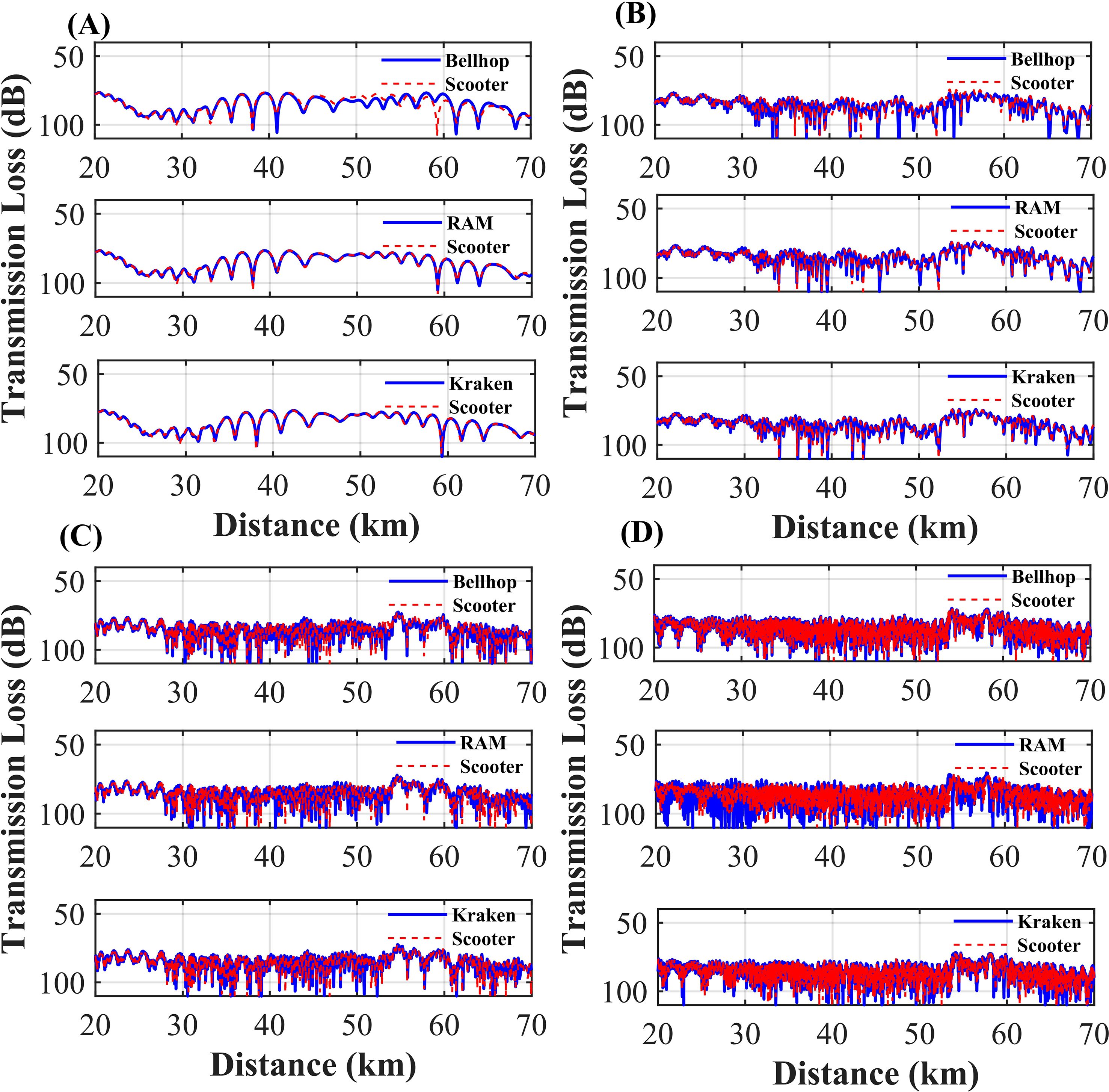
Figure 5. Transmission loss comparison for deep-sea simulations over a 50 km range. (A) Comparison results at 10 Hz, (B) Comparison results at 50 Hz, (C) Comparison results at 100 Hz, (D) Comparison results at 500 Hz.

Table 4

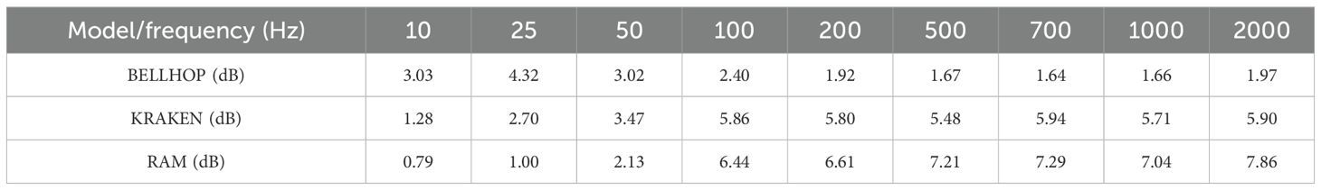
Table 4. Root mean square error (RMSE) analysis for deep-sea simulations.

Figure 6

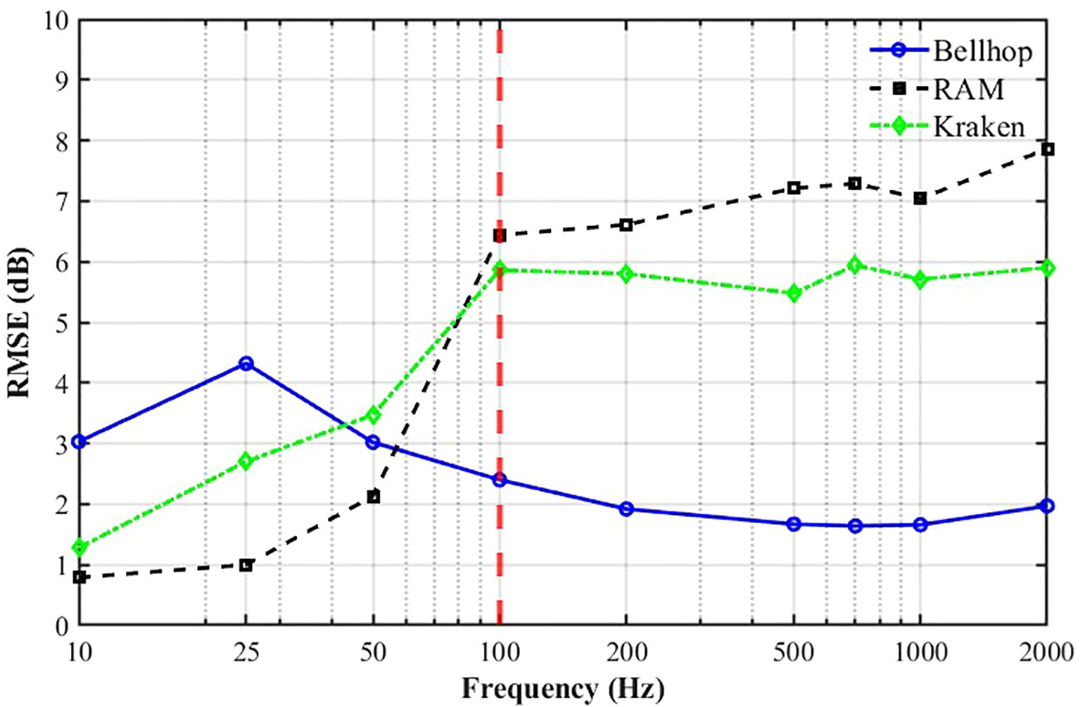
Figure 6. Root mean square error (RMSE) comparison for deep-sea simulations over a 50 km range. The red dashed line indicates the frequency threshold separating the low-frequency (RAM-dominant) and high-frequency (BELLHOP-dominant) regions.

Through analysis of deep-sea environmental conditions, the frequency adaptability of the models is as follows: for frequencies below 100 Hz, BELLHOP exhibits the poorest simulation performance, followed by KRAKEN, while RAM achieves the highest accuracy. For frequencies above 100 Hz, RAM’s accuracy is lower than KRAKEN’s, with BELLHOP demonstrating the best performance.

In summary, for deep-sea frequency adaptability analysis, BELLHOP is more suitable for simulations above 100 Hz, while RAM is recommended for simulations below 100 Hz.

4 Simulation and analysis under sloping conditions

Previous studies primarily focused on flat seabed environments. However, real deep-sea terrains are often non-flat, and slopes significantly affect sound propagation, particularly at low frequencies, where range-dependent effects may disrupt modal stability. To evaluate the adaptability of the BELLHOP, KRAKEN, and RAM models under sloping conditions, we conducted simulations for different seabed slopes and performed comparative analyses. Based on the RMSE results, a slope angle of approximately 6.5° was identified as the threshold distinguishing gentle and steep seabed conditions. Slopes smaller than 6.5° were classified as gentle, while those greater than 6.5° were considered steep. The simulation setup included a sound source at 100 m depth, a receiver at 30 m depth, and a constant sound speed of 1500 m/s. Three slopes were considered: (1) a 15 km range with depth decreasing from 200 m to 1 m; (2) a 4 km range with depth decreasing from 400 m to 1 m (slope 5.71°); (3) a 4 km range with depth decreasing from 600 m to 1 m (slope 8.51°); and (4) a 4 km range with depth decreasing from 490 m to 1 m (slope 7°). Transmission loss at the receiver was analyzed, with RMSE evaluated over 0.5–12 km for the 15 km scenario and 0.5–3.5 km for the 4 km scenarios, accounting for shadowing effects.

4.1 Simulation with gentle slope

To evaluate the adaptability of the BELLHOP, KRAKEN, and RAM models in gentle slope (<6.5°) terrains, simulations were conducted for slopes of 0.76° and 5.71°. The gentle slope terrains are shown in Figure 7. The impact of gentle slopes on model performance was assessed by comparing transmission loss with a benchmark solution. Transmission loss comparisons are presented in Figures 8, 9, with statistical error results shown in Tables 5, 6; Figure 10.

Figure 7

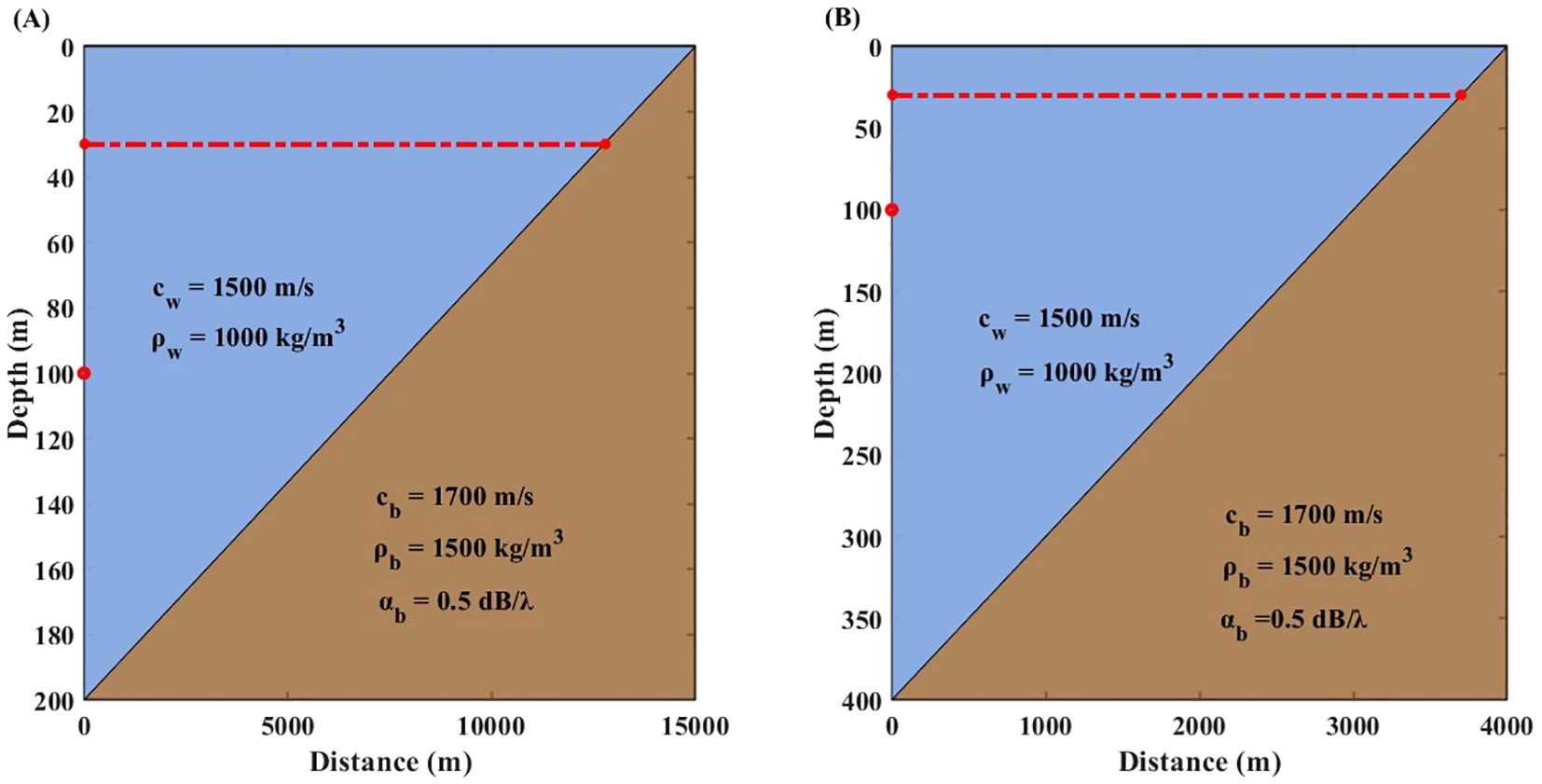
Figure 7. Topography and sound speed profiles for gentle-slope simulations. The red dot denotes the sound source position, and the yellow line denotes the receiver positions. (A) Slope of 0.76°; (B) Slope of 5.71°.

Figure 8

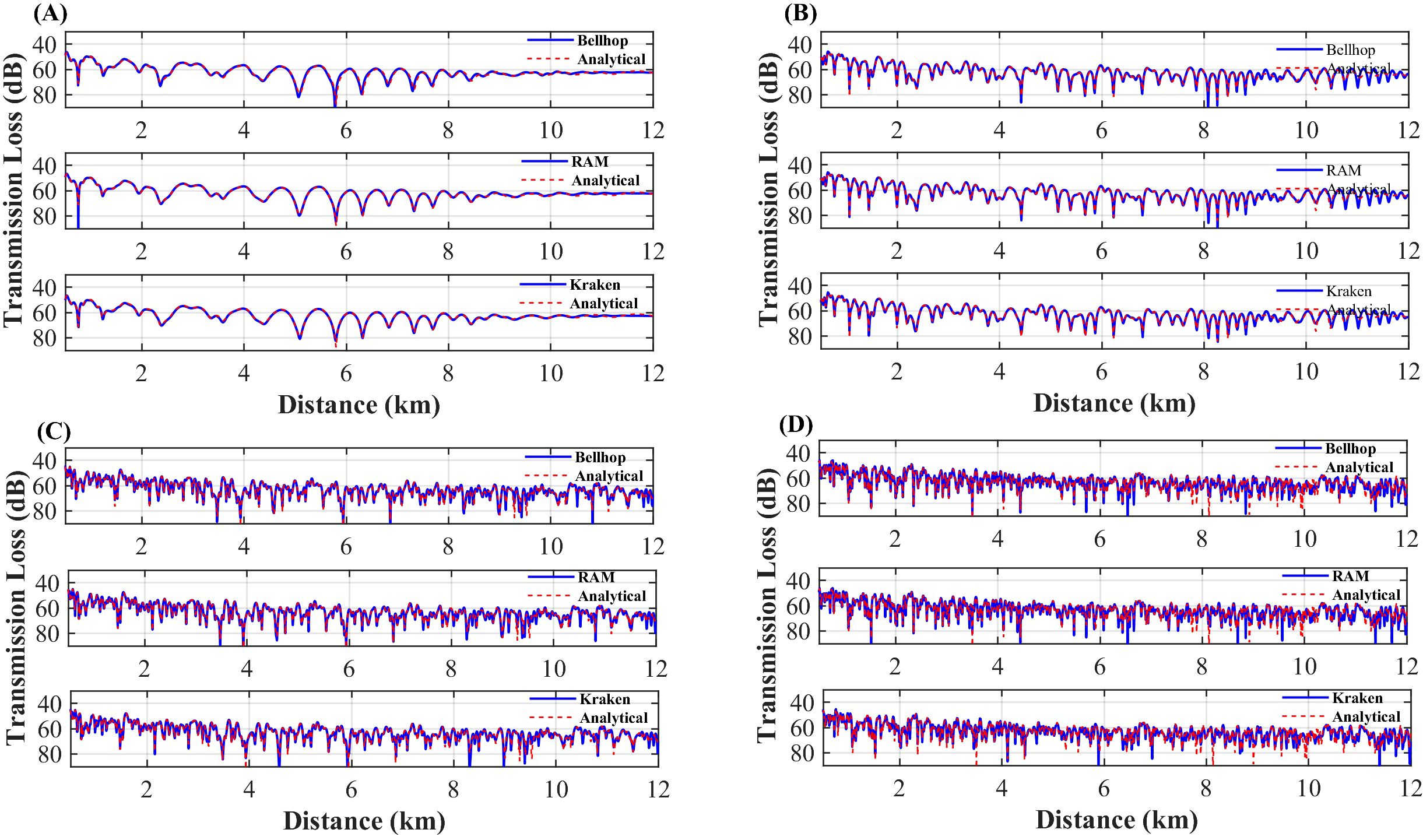
Figure 8. Transmission loss comparison for simulations with a 0.76° slope. (A) Comparison results at 50 Hz, (B) Comparison results at 100 Hz, (C) Comparison results at 200 Hz, (D) Comparison results at 300 Hz.

Figure 9

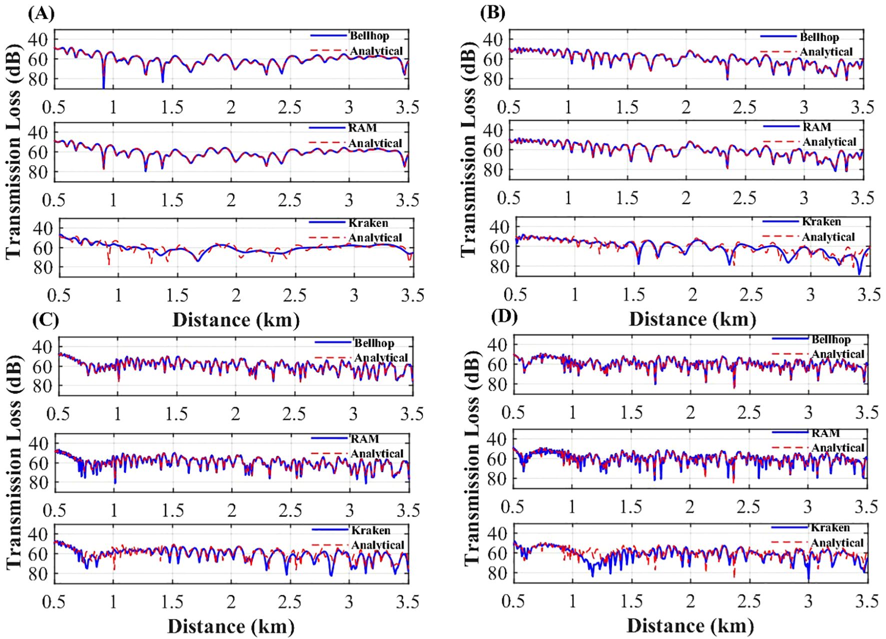
Figure 9. Transmission loss comparison for simulations with a 5.71° slope. (A) Comparison results at 50 Hz, (B) Comparison results at 100 Hz, (C) Comparison results at 200 Hz, (D) Comparison results at 300 Hz.

Table 5

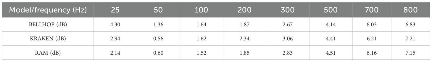
Table 5. Root mean square error (RMSE) comparison for simulations with a 0.76° slope.

Table 6

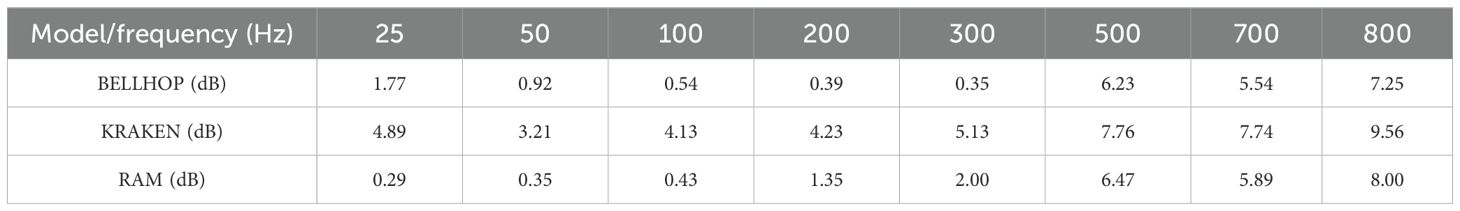
Table 6. Root mean square error (RMSE) comparison for simulations with a 5.71° slope.

Figure 10

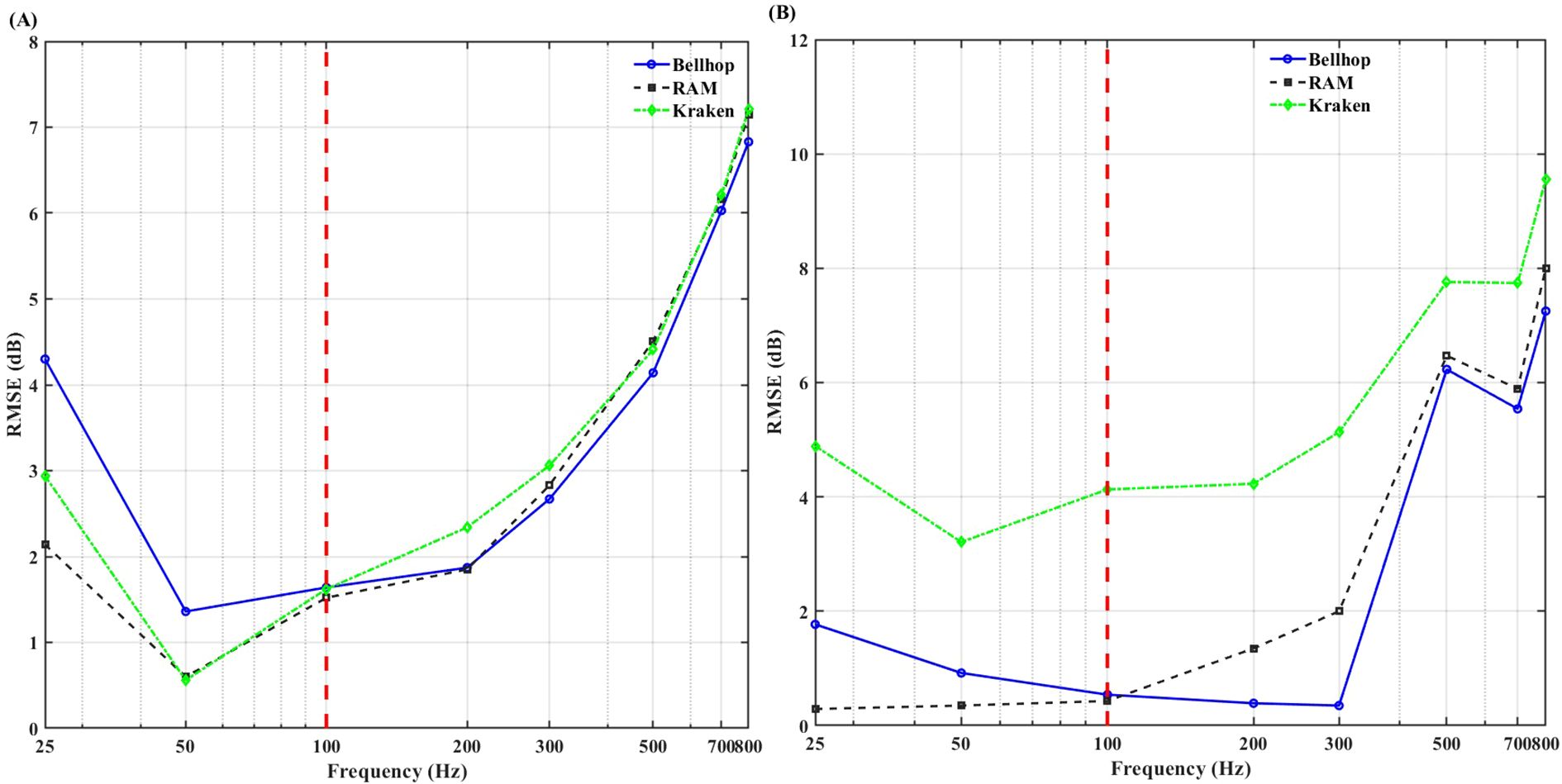
Figure 10. Comparison of root mean square error (RMSE) for gentle-slope simulations. The red dashed line indicates the frequency threshold separating the low-frequency (RAM-dominant) and high-frequency (BELLHOP-dominant) regions (A) Slope of 0.76°; (B) Slope of 5.71°.

For the 0.76° slope, RAM and KRAKEN demonstrate excellent performance at frequencies up to 100 Hz, with RMSEs ranging from 0.60 to 2.14 dB and from 0.56 to 2.94 dB, respectively, clearly outperforming BELLHOP, which reaches a maximum RMSE of 4.30 dB. At frequencies exceeding 100 Hz, RAM and KRAKEN exhibit comparable accuracy, whereas BELLHOP provides superior performance. Similarly, for the 5.71° slope, RAM maintains an RMSE of 1 dB or less for frequencies up to 100 Hz, outperforming KRAKEN, which has a maximum RMSE of 4.89 dB. At frequencies above 100 Hz, BELLHOP achieves the highest accuracy.

In gentle slope terrains, RAM excels at low frequencies (<100 Hz), BELLHOP is superior at high frequencies (>100 Hz), and KRAKEN is only suitable for very gentle slopes (0.76°). Future studies will explore the impact of steeper slopes on model performance.

4.2 Simulation with steep slope

To evaluate the adaptability of the BELLHOP, KRAKEN, and RAM models in steep slope (>6.5°) terrains, simulations were conducted for slopes of 7° and 8.51°. The steep slope terrains are shown in Figure 11. The impact of steep slopes on model performance was assessed by comparing transmission loss with a benchmark solution. Transmission loss comparisons are presented in Figures 12, 13, with statistical error results shown in Tables 7, 8; Figure 14.

Figure 11

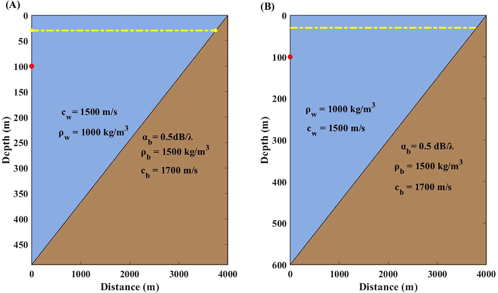
Figure 11. Topography and sound speed profiles for steep-slope simulations. The red dot denotes the sound source position, and the yellow line denotes the receiver positions. (A) Slope of 7°; (B) Slope of 8.51°.

Figure 12

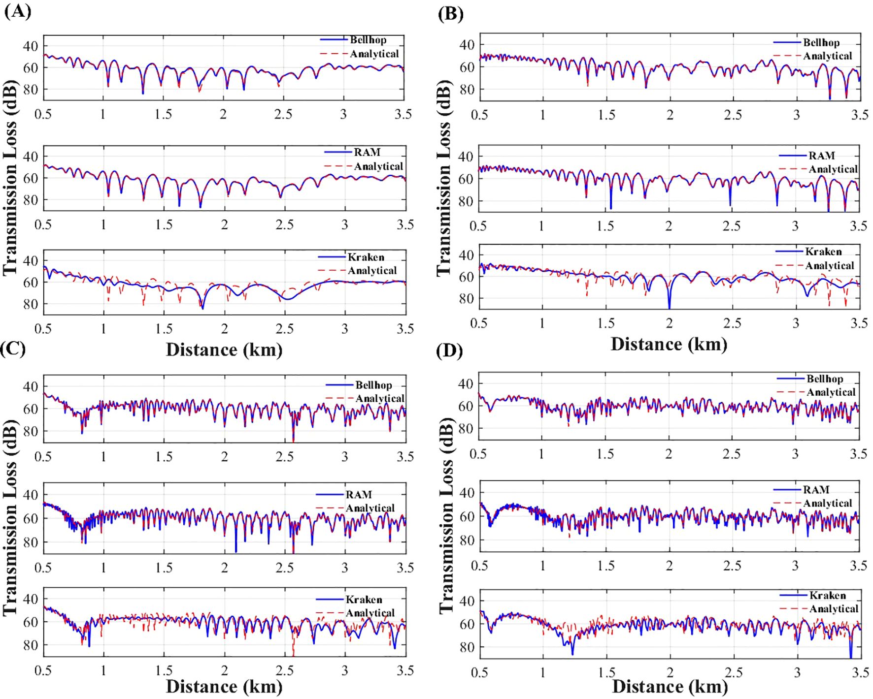
Figure 12. Transmission loss comparison for simulations with a 7° slope. (A) Comparison results at 50 Hz, (B) Comparison results at 100 Hz, (C) Comparison results at 200 Hz, (D) Comparison results at 300 Hz.

Figure 13

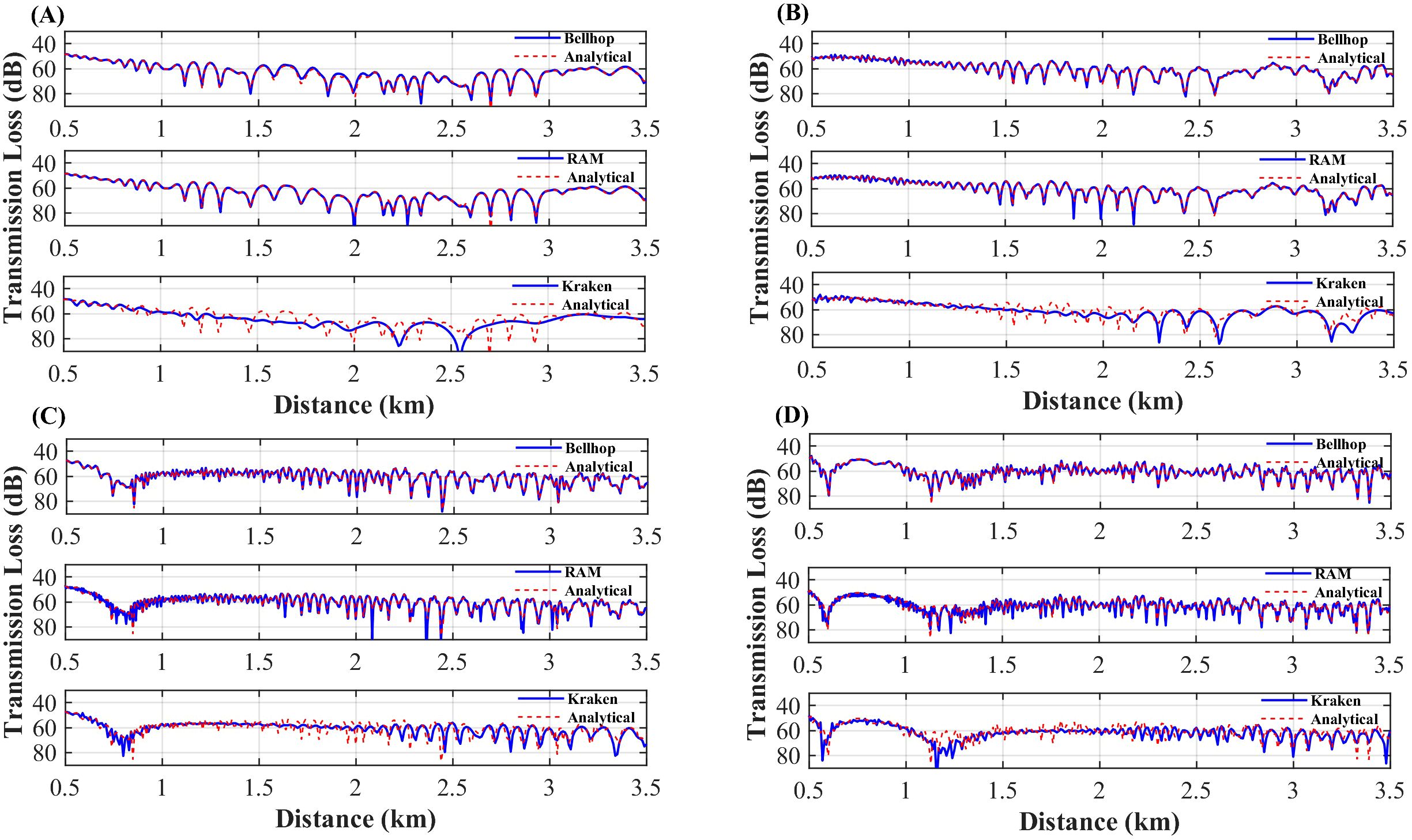
Figure 13. Transmission loss comparison for simulations with a 8.51° slope. (A) Comparison results at 50 Hz, (B) Comparison results at 100 Hz, (C) Comparison results at 200 Hz, (D) Comparison results at 300 Hz.

Table 7

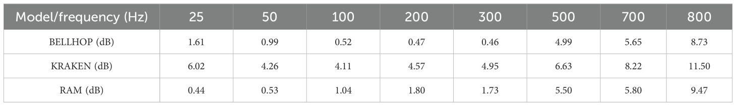
Table 7. Root mean square error (RMSE) comparison for simulations with a 7° slope.

Table 8

Table 8. Root mean square error (RMSE) comparison for simulations with a 8.51° slope.

Figure 14

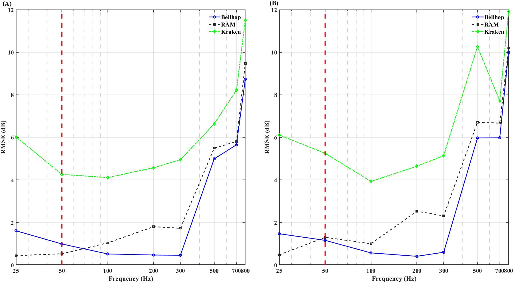
Figure 14. Comparison of root mean square error (RMSE) for steep-slope simulations. The red dashed line indicates the frequency threshold separating the low-frequency (RAM-dominant) and high-frequency (BELLHOP-dominant) regions (A) Slope of 7°; (B) Slope of 8.51°.

For the 7° slope, RAM demonstrates excellent performance at frequencies up to 50 Hz, with RMSEs ranging from 0.44 to 0.53 dB, outperforming BELLHOP. At frequencies above 50 Hz, BELLHOP achieves higher simulation accuracy than RAM. Similarly, for the 8.51° slope, RAM maintains strong adaptability at frequencies up to 50 Hz, with RMSEs between 0.48 and 1.30 dB relative to the benchmark solution. In contrast, KRAKEN exhibits high RMSE values across the entire frequency range, particularly at frequencies exceeding 50 Hz, where BELLHOP outperforms RAM.

In steep slope terrains, RAM excels at low frequencies (<50 Hz), BELLHOP is superior at high frequencies (>50 Hz), and KRAKEN is unsuitable for steep slope simulations.

4.3 Summary of model applicability across sloping conditions

Simulation results in gentle slope environments indicate that at frequencies below 100 Hz, RAM outperforms BELLHOP in simulation accuracy. Analysis reveals that BELLHOP’s lower energy predictions at low frequencies stem from its ray-based modeling approach, which fails to capture modal propagation characteristics, omitting the energy contribution of low-frequency modes. BELLHOP’s simulations account only for direct and limited reflected paths, neglecting the energy distribution of modal propagation. Furthermore, under uniform sound speed profile conditions, the absence of sound speed gradients results in frequent interactions with the sea surface and seabed, leading to additional energy loss due to boundary absorption, with overall energy significantly lower than RAM’s results. For frequencies above 100 Hz, BELLHOP’s simulation accuracy surpasses that of KRAKEN and RAM. RMSE analysis plots further confirm that RAM and KRAKEN exhibit higher adaptability in the low-frequency band, while BELLHOP’s accuracy improves progressively in the high-frequency band. Therefore, in gentle -slope acoustic simulations, RAM is recommended for frequencies below 100 Hz to ensure higher accuracy, while BELLHOP is preferred for frequencies above 100 Hz.

In steep-slope marine environments, simulation results demonstrate that frequency significantly impacts model performance. For frequencies below 50 Hz, RAM outperforms both KRAKEN and BELLHOP. Analysis indicates that BELLHOP, via ray tracing, and RAM, via the parabolic equation, effectively capture acoustic path variations and energy distributions under large-slope topographies, demonstrating higher adaptability. For frequencies above 50 Hz, BELLHOP outperforms RAM, as high-frequency acoustic propagation aligns more closely with geometric optics, enabling BELLHOP’s ray theory to more accurately model multipath effects and slope reflection paths. RMSE analysis plots further reveal that KRAKEN’s applicability in large-slope environments is limited, with significantly increased RMSE, particularly in the low-frequency band. Therefore, in large-slope environments, RAM is recommended for simulations below 50 Hz, while BELLHOP is preferred for frequencies above 50 Hz to achieve higher accuracy.

5 Discussion

This study quantitatively evaluates the performance of three underwater acoustic propagation models—BELLHOP (ray-based), RAM (parabolic equation), and KRAKEN (normal mode)—in shallow flat seabeds, deep-sea flat oceans, and sloped seabed environments. Our findings align with prior research while offering novel insights into model applicability across varying frequencies and bathymetric conditions. Oliveira et al. (2021) demonstrated that RAM maintains stable performance in complex shallow-water environments with varying bathymetry, whereas ray-based models like BELLHOP are more sensitive to environmental changes. Similarly, Wynn-Simmonds et al. (2025) noted that RAM balances accuracy and computational efficiency in mid-frequency ranges, while BELLHOP excels at high frequencies. Our results confirm that RAM performs better in shallow-water and gentle-slope (<6.5°) scenarios at low frequencies (<100 Hz), while BELLHOP outperforms RAM and KRAKEN at high frequencies (>200 Hz) in shallow water and above 50 Hz in steep-slope (>6.5°) environments. In deep-sea flat environments, BELLHOP is more suitable above 100 Hz, and RAM performs better below 100 Hz.

The novelty of this study lies in establishing frequency- and slope-dependent performance boundaries. For gentle slopes (<6.5°), BELLHOP is suitable for frequencies above 100 Hz, and RAM for frequencies below 100 Hz. For steep slopes (>6.5°), BELLHOP is preferable above 50 Hz, while RAM is more accurate below 50 Hz. These thresholds provide practical guidance for model selection based on environmental complexity and frequency range, complementing the qualitative insights of prior studies.

Conducted in controlled settings to isolate frequency and slope effects, this study is limited by idealized sound speed profiles and the absence of three-dimensional seabed roughness analysis. Comprehensive uncertainty analysis was also not performed. Future work should validate these findings through field experiments and extend analyses to three-dimensional environments. In conclusion, this study addresses the prior lack of quantitative model assessments, offering clear guidelines for researchers and engineers to select appropriate models based on specific marine environments and frequency ranges.

6 Conclusions

This study systematically evaluates the applicability of three acoustic models—BELLHOP (based on ray tracing), KRAKEN (coupled mode), and RAM (parabolic equation model)—across four typical marine environments: shallow-water flat seabed, deep-sea flat ocean, gentle -slope terrain (slope < 6.5°), and steep-slope terrain (slope > 6.5°). By comparing their simulation performance against benchmark models (Scooter for flat terrains and analytical solutions for sloped terrains), the study analyzes the models’ performance under varying frequency and topographic conditions, revealing their strengths and limitations. The key findings are as follows:

In a flat shallow-sea environment for a 4 km propagation range, when frequencies are below 200 Hz, KRAKEN and RAM exhibit excellent simulation accuracy, with RMSE values of 0.48–1.6 dB and 0.49–0.79 dB, respectively. Conversely, BELLHOP demonstrates strong simulation capability for frequencies above 200 Hz, with RMSE reduced to within 0.5 dB However, at a 10 km range for frequencies below 200 Hz, BELLHOP’s simulation accuracy is significantly lower than RAM’s, with RMSE values of 1.41–4.22 dB compared to 0.69–0.89 dB. This discrepancy arises from increased sound field complexity due to longer propagation distances: in the 4 km near field, modal effects are simple, whereas in the 10 km far field, low-frequency modal diffusion and attenuation intensify. RAM’s parabolic equation method effectively models far-field sound propagation, while BELLHOP’s ray theory fails to capture these effects, resulting in significantly steep RMSE.

In a flat deep-sea environment, BELLHOP exhibits optimal simulation accuracy for frequencies above 100 Hz, with RMSE reduced to within 2dB. However, for frequencies below 100 Hz, RAM outperforms KRAKEN, with RMSE values of 0.79–2.13 dB and 1.28–3.47 dB, respectively, indicating that the complexity of sound speed profiles (e.g., the SOFAR channel) in deep-sea environments impacts KRAKEN’s modal propagation simulations. Furthermore, when frequencies exceed 100 Hz, RAM’s applicability diminishes, with RMSE increasing to approximately 7 dB, resulting in the poorest simulation performance.

In gentle-slope environments, for frequencies below 100 Hz, RAM exhibits the highest simulation accuracy. When frequencies exceed 100 Hz, BELLHOP achieves the best accuracy. This indicates that in gentle -slope topographies under high-frequency conditions, BELLHOP delivers optimal simulation performance.

In large-slope environments, for frequencies below 50 Hz, RAM outperforms BELLHOP in simulation accuracy, with RMSE within 1 dB, while KRAKEN’s adaptability significantly declines, indicating its unsuitability for large-slope topography simulations. When frequencies exceed 50 Hz, BELLHOP achieves the highest simulation accuracy among the three models, followed by RAM.

The results from the preceding sections highlight that terrain slope and frequency significantly influence model applicability. Specific recommended usage scenarios are summarized in Table 9.

Table 9

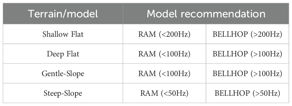
Table 9. Recommended model usage for different scenarios.

These findings provide a theoretical basis for selecting acoustic models under similar topographic and frequency conditions. However, the models’ applicability in more complex environments, such as strongly stratified water columns or irregular terrains, requires further investigation. Future research could explore the performance of these models in complex topographic settings to enhance their generalizability.

Data availability statement

The original contributions presented in the study are included in the article/supplementary material. Further inquiries can be directed to the corresponding author.

Author contributions

ML: Writing – original draft. CC: Writing – review & editing, Supervision. XF: Investigation, Writing – review & editing. CW: Data curation, Writing – review & editing. HW: Investigation, Writing – review & editing.

Funding

The author(s) declare financial support was received for the research and/or publication of this article. The study is supported by the National Natural Science Foundation of China (Nos. 52471366).

Acknowledgments

We express our sincere gratitude to the Northwestern Polytechnical University School of Marine Science and Technology and the Key Laboratory of Ocean Acoustics and Sensing, Ministry of Industry and Information Technology, for providing essential computational resources and technical support. We also thank our colleagues for their valuable discussions and feedback throughout the study. This work was supported by the National Natural Science Foundation of China (Grant No. 52471366).

Conflict of interest

The authors declare that the research was conducted in the absence of any commercial or financial relationships that could be construed as a potential conflict of interest.

Generative AI statement

The author(s) declare that no Generative AI was used in the creation of this manuscript.

Any alternative text (alt text) provided alongside figures in this article has been generated by Frontiers with the support of artificial intelligence and reasonable efforts have been made to ensure accuracy, including review by the authors wherever possible. If you identify any issues, please contact us.

Publisher’s note

All claims expressed in this article are solely those of the authors and do not necessarily represent those of their affiliated organizations, or those of the publisher, the editors and the reviewers. Any product that may be evaluated in this article, or claim that may be made by its manufacturer, is not guaranteed or endorsed by the publisher.

References

Ballard M. S., Goldsberry B. M., and Isakson M. J. (2015). Normal mode analysis of three-dimensional propagation over a small-slope cosine shaped hill. J. Comput. Acoust 23, 1550005. doi: 10.1142/S0218396X15500058

Crossref Full Text | Google Scholar

Chai Z., Wang Q., Zhu H., Cui Z., and Tu H. (2022). Effects of non-ideal seabed topography on low frequency sound propagation in shallow sea. J. Physics: Conf. Ser. 2486, 012080. doi: 10.1088/1742-6596/2486/1/012080

Crossref Full Text | Google Scholar

Chen W., Zhang Y., Liu Y., Wu Y., Zhang Y., and Ren K. (2022). Observation of a mesoscale warm eddy impacts acoustic propagation in the slope of the South China Sea. Front. Mar. Sci. 9. doi: 10.3389/fmars.2022.1086799

Crossref Full Text | Google Scholar

Collins M. D. (1993). A split-step Pade solution for the parabolic equation method. J. Acoust Soc. Am. 93, 1736–1742. doi: 10.1121/1.406739

Crossref Full Text | Google Scholar

Dahl P. H. and Dall'Osto D. R. (2017). On the underwater sound field from impact pile driving: Arrival structure, precursor arrivals, and energy streamlines. J. Acoust Soc. Am. 142, 1141–1155. doi: 10.1121/1.4999060

PubMed Abstract | Crossref Full Text | Google Scholar

Deane G. B. and Tindle C. T. (1992). A three-dimensional analysis of acoustic propagation in a penetrable wedge slice. J. Acoust Soc. Am. 92, 1583–1592. doi: 10.1121/1.403900

Crossref Full Text | Google Scholar

Jensen F. B., Kuperman W. A., Porter M. B., and Schmidt H. (2011). Computational Ocean Acoustics (Springer, New York, USA).

Google Scholar

King B., Miller J. H., Potty G. R., Lopez Case J. F., Chen T.-T., and Lin Y. (2023). Impacts of seafloor characteristics on sound propagation in a seamount environment. J. Acoustical Soc. America 154, A167–A16A. doi: 10.1121/10.0023151

Crossref Full Text | Google Scholar

Li Z., Piao S., Zhang M., and Gong L. (2022). Influence of range-dependent sound speed profile on position of convergence zones. Remote Sens. 14, 6314. doi: 10.3390/rs14246314

Crossref Full Text | Google Scholar

Lin Y.-T. and Duda T. F. (2012). A higher-order split-step Fourier parabolic-equation sound propagation solution scheme. J. Acoustical Soc. America 132, EL61–EEL7. doi: 10.1121/1.4730328

PubMed Abstract | Crossref Full Text | Google Scholar

Oliveira T. C. A., Lin Y. T., and Porter M. B. (2021). Underwater sound propagation modeling in a complex shallow water environment. Front. Mar. Sci. 8. doi: 10.3389/fmars.2021.751327

Crossref Full Text | Google Scholar

Porter M. B. (1992). The KRAKEN normal mode program (NRL Report 9929). Naval Research Laboratory, Washington, DC, USA.

Google Scholar

Porter M. B. and Bucker H. P. (1987). Gaussian beam tracing for computing ocean acoustic fields. J. Acoust Soc. Am. 82, 1349–1359. doi: 10.1121/1.395269

Crossref Full Text | Google Scholar

Possenti L., De Nooijer L., De Jong C., Lam F. P., Beelen S., Bosschers J., et al. (2024). The present and future contribution of ships to the underwater soundscape. Front. Mar. Sci. 11. doi: 10.3389/fmars.2024.1252901

Crossref Full Text | Google Scholar

Wu S., Li Z., Qin J., Wang M., and Li W. (2022). The effects of sound speed profile to the convergence zone in deep water. J. Mar. Sci. Eng. 10, 424. doi: 10.3390/jmse10030424

Crossref Full Text | Google Scholar

Wynn-Simmonds S., Vincent C., Mathias D., and Richard G. (2025). Comparative analysis of underwater acoustic propagation models: Evaluating the trade-off between accuracy and computational demands for coastal noise predictions. J. Mar. pollut. Bull. 215, 117905. doi: 10.1016/j.marpolbul.2025.117905

PubMed Abstract | Crossref Full Text | Google Scholar