Abstract
Introduction:
Marine litter is an issue affecting all regions of the World Ocean. To address the problem of World Ocean pollution, it is essential first and foremost to develop observation methodologies capable of providing objective assessments of marine litter density and its sources.
Methods:
One of the most accessible yet still objective observation methods is visual imaging of the ocean surface followed by the analysis of the imagery acquired. The goal of our study is to develop a method for analyzing marine surface imagery capable of detecting anomalies, given that some of the anomalies would represent floating marine litter.
Results:
For this purpose, we apply our algorithm based on artificial neural networks trained within the contrastive learning framework, along with a classifier based on supervised machine learning method for analyzing optical imagery of sea surface.
Discussion:
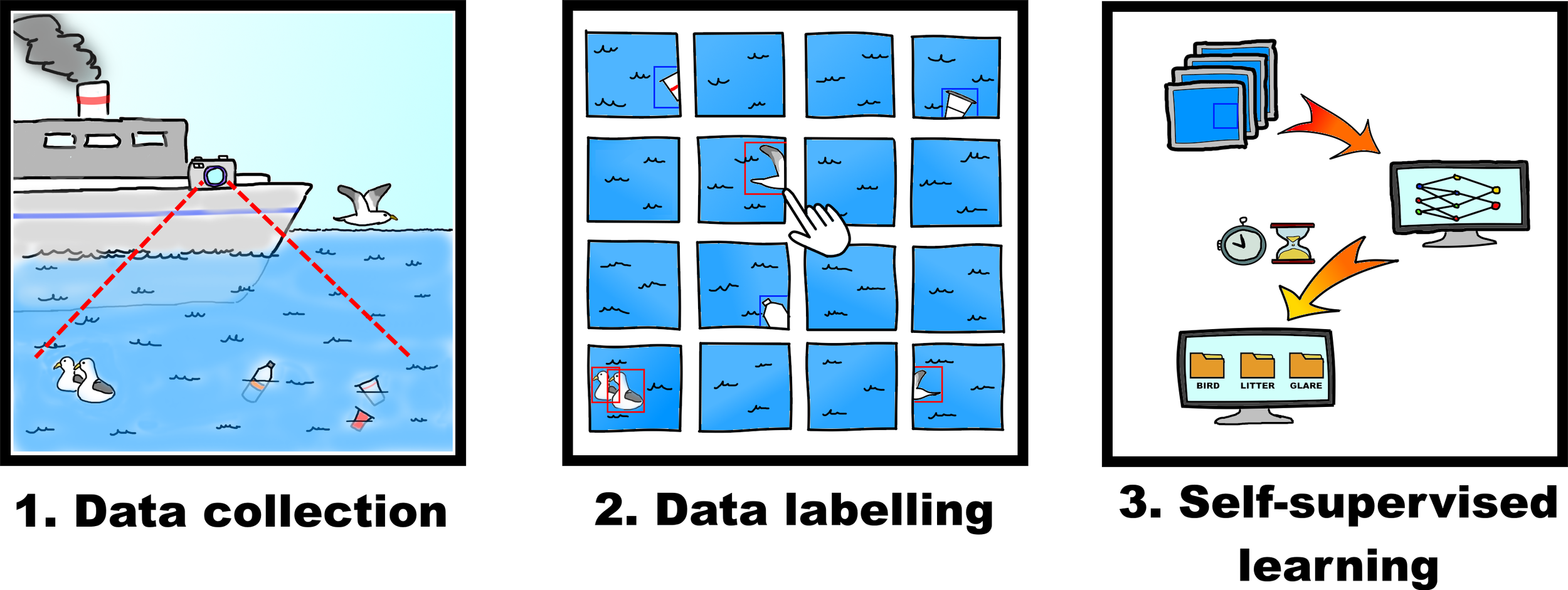
The approach we present in this study is capable of detecting anomalies such as floating marine litter, birds, unusual glare, and other atypical visual phenomena. We explored capabilities of the artificial neural networks we use in this study within two training approaches with subsequent comparison of the results. Within our sampling approach, we propose to utilize the ergodic property of sea wave fields, leading to significant spatial autocorrelation of image elements with a substantial correlation radius.
Graphical Abstract
1 Introduction
Marine litter represents a globally recognized environmental challenge addressed by international maritime organizations and conservation conventions. Detection of marine litter is complicated by object diversity, varying decomposition states, small size, partial submersion, color degradation, surface camouflage, and adverse observation conditions.
According to the United Nations Environment Program (UNEP), marine litter encompasses any persistent, manufactured or processed solid material discarded in marine and coastal environments (Galgani et al., 2023). Analyses consistently show that plastics comprise the vast majority of all identified litter, often reaching 68–96% in various marine environments (Galgani et al., 2015; Raju et al., 2025). This pollution threatens marine biodiversity through accumulation in coastal areas (Ershova et al., 2024), aquatic ecosystems (Katsanevakis, 2014), and formation of oceanic garbage patches (Lebreton et al., 2018), as documented by expeditions worldwide (González-Fernández et al., 2022) (Pogojeva et al., 2021). Marine litter damages organisms through entanglement and ingestion while altering benthic habitats and facilitating invasive species transport (Derraik, 2002; Aliani and Molcard, 2003; Boerger et al., 2010; Gall and Thompson, 2015).
Floating litter, transported by winds and currents, indicates litter pathways until objects settle on the seabed, wash ashore, or degrade (Andrady, 2015). This study focuses on macro-litter objects—litter exceeding 2.5 cm according to international classification (Lippiatt et al., 2013)—as microscopic fragments like microplastics cannot be captured through direct video recording.
Traditional marine litter monitoring relies on visual observations from vessels and aircraft, trawling operations, and remote sensing using radar systems. Visual monitoring typically involves trained observers on research vessels conducting auxiliary studies (Derraik, 2002; Lippiatt et al., 2013), requiring substantial time, labor, and specialized expertise, resulting in infrequent coverage of limited ocean areas. Trawling provides quantitative sampling but is labor-intensive and spatially restricted. To overcome these limitations, the scientific community has increasingly turned to remote sensing and Artificial Intelligence (Veettil et al., 2022; Kako et al., 2025; Gayathrri et al., 2025). Recent advancements have demonstrated the power of deep learning models for litter detection using data from various platforms, including drones (Garcia-Garin et al., 2020; Jeong et al., 2024), aircraft, and satellites (Srinivasa, 2025). Architectures such as YOLO, R-CNN, and UNet have achieved high accuracy in classifying and quantifying marine litter (Prakash and Zielinski, 2025; Raju et al., 2025).
Recent advances in deep learning have revolutionized litter recognition through artificial neural networks. Convolutional neural network architectures, particularly YOLO (You Only Look Once) and R-CNN (Region-based Convolutional Neural Networks) families, demonstrate superior performance in object detection and classification tasks (Watanabe et al., 2019; Kylili et al., 2021; Xue et al., 2021; de Vries, 2022). YOLO models excel in real-time detection by simultaneously predicting object locations and classifications, while R-CNN variants provide high accuracy through region proposal mechanisms. These modern approaches significantly outperform classical computer vision methods in marine litter identification.
Despite these advances, a significant challenge remains: most state-of-the-art supervised models require vast, manually annotated datasets for training. The creation of such datasets is a major bottleneck due to the sheer diversity of litter types, shapes, and environmental conditions (Topouzelis et al., 2021; Kako et al., 2025). This dependency limits the scalability and widespread adoption of automated monitoring systems. Our work aims to address this gap by developing a method that can learn to detect litter without requiring large, pre-labeled training examples.
Automated visual monitoring could enable widespread implementation aboard commercial vessels through bow-mounted cameras and specialized software for optical image analysis. However, implementing automated surveillance in marine environments presents significant organizational and technical challenges (Lippiatt et al., 2013).
Therefore, the primary objectives of this study are as follows. Firstly, we aim to develop a novel method for detecting anomalies in sea surface imagery using an artificial neural network trained within a contrastive learning framework. Secondly, we propose and implement a unique data sampling strategy that utilizes the ergodic property of sea wave fields, enabling the model to be trained effectively on primarily unlabeled data.
This paper is structured as follows. We begin by describing the data collected during our marine expedition and the analytical methods employed. We then present an exploratory data analysis, followed by a detailed account of the data preparation, model training, and application. Finally, the conclusion summarizes our findings, discusses the applicability of our approach, and outlines directions for future research.
2 Materials and methods
2.1 Collected data
Our study utilized video data recorded during a scientific expedition in the Arctic Ocean conducted in autumn 2023. The research vessel “Dalnie Zelentsy” departed from Murmansk port and traveled through the Barents and Kara Seas toward the Novaya Zemlya archipelago shores. The collected videos, as well as the observational journal with GPS coordinates and image datasets with labelled objects, are published on Kaggle, an online data science community (Bilousova et al., 2025). The expedition route is illustrated in Figure 1.
Figure 1
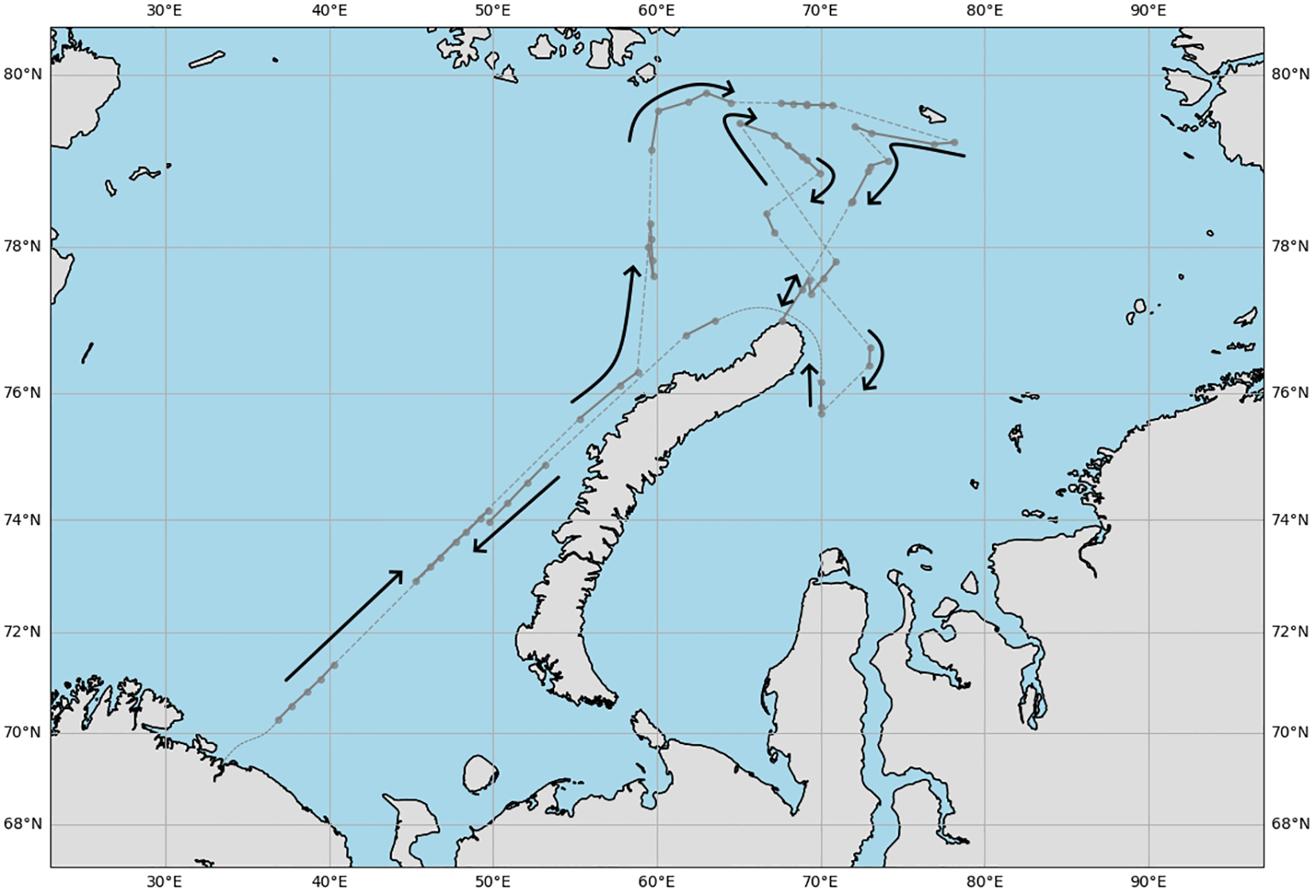
The route of the Dalniye Zelentsy expedition in the Barents and Kara Seas in September 2023. The gray dotted line indicates the approximate route of the vessel, where a GPS track was not recorded. Black arrows indicate the vessel’s direction of travel.
Video recordings of the sea surface were captured while the vessel was underway during daylight hours. The camera was mounted on the port side at approximately 5.5 meters height, with a field of view spanning 6–15 meters in width and approximately 25 meters in length from the vessel. The recording configuration, the mounting location, and a photograph of the attached camera is depicted in Figures 2a–c.
Figure 2
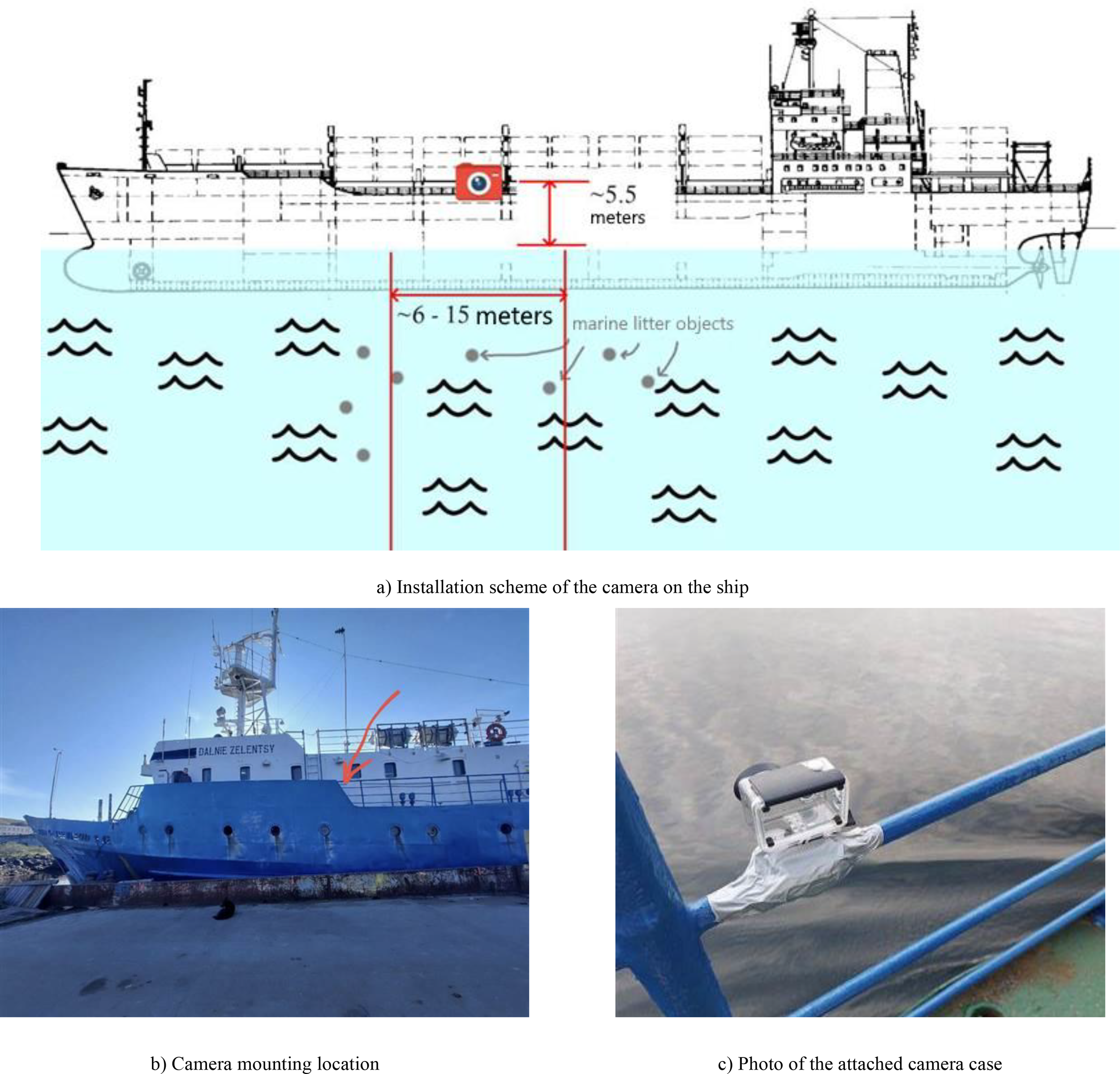
(a) Installation scheme of the camera on the ship. (b) Camera mounting location. (c) Photo of the attached camera case.
The total recorded video material exceeded 136 hours duration. Original data was provided as compressed video files created through the following technical process: recording was conducted at 1 frame per second, with captured frames subsequently assembled into single video files that play back at 30 frames per second. Consequently, 1 minute of real time corresponds to 60 frames, equivalent to exactly 2 seconds of video playback.
The camera was set on the ship’s board at the height of approximately 5.5 meters and filmed to the distance about 6–15 meters in the front of it. Typical filming sessions aboard the vessel lasted approximately 2 hours, resulting in compressed videos averaging 4 minutes in length. The image resolution of all photos is 3840×2160 pixels.
2.2 Description of ML methods used in the paper
This section provides a description of the machine learning methods and models employed for data processing and analysis in the current work.
2.2.1 Contrastive networks and momentum contrast
Contrastive learning represents a promising approach in self-supervised learning that focuses on training models to identify similarities between different parts of the same image. A key advantage of contrastive learning is its ability to learn from vast amounts of unlabeled data, making this approach particularly valuable when labeled data is limited. Contrastive networks demonstrate high efficiency across various computer vision tasks, including image classification, segmentation, and object detection. Another notable feature is their ability to learn without supervision, eliminating the need for preliminary data labeling. After training the model on training data, a CatBoost classifier (Prokhorenkova et al., 2018) will be trained and applied to the validation dataset.
MoCo (Momentum Contrast) is a contrastive learning method proposed in 2020 by researchers from Facebook AI Research and UIUC. The core concept involves simultaneously using two instances, or branches, of the same network: one network updates through backpropagation, while the other updates using momentum from the first network’s parameters.
Training contrastive learning models involves minimizing the contrastive loss function. This requires creating arrays of positive and negative pairs. Contrastive loss measures sample pair similarity in the representation space; the loss value decreases as data instances move closer to their positive keys (positive pairs) and further from negative keys (negative pairs). In this study, ResNet50 architecture (He et al., 2020) served as both the encoder and momentum encoder.
Below is a brief mathematical explanation of the MoCo method. Let us denote a data sample as kq, and the representation of this instance, computed by the encoder, as q = fq(kq).
Assume that there is one positive key among them, corresponding to the vector. The loss function used is InfoNCE (Noise Contrastive Estimation) in (Equation 1):
Here, q is the query vector, is the positive key, are the keys in the dictionary, and τ is the temperature parameter.
In the software implementation of the MoCo method, we used two similar types of cross-entropy loss function (more details in Section 5) – InfoNCE and a type of cross-entropy – binary cross-entropy (BCE). The formula for the BCE is as follows (Equation 2):
where yi are the true labels, and pi are the predicted probabilities.
One obvious way to circumvent this feature would be to use the same encoder for both and . However, MoCo proposed a different approach—momentum-based update. Let the parameters of the encoders for queries and keys be denoted as и respectively. Then the update iteration for the key encoder, using a momentum-based encoder, can be written as (Equation 3):
From the formula above, it is evident that by varying the momentum coefficient m, one can influence the rate of separation between positive and negative pairs and, consequently, the learning step.
The advantage of MoCo lies in the fact that in MoCo, the batch size is not dependent on the number of negative pairs, and the model does not require a large batch size to have a sufficient number of negative samples. As a result, MoCo does not significantly lose performance when the batch size is reduced.
From a software implementation perspective, the model works as follows: both branches of the network, which are identical in terms of their ResNet50 architecture, receive the same data batches as input. The model’s core encoder is trained using stochastic gradient descent.
2.2.2 DBSCAN
DBSCAN (Density-Based Spatial Clustering of Applications with Noise) (Ester et al., 1996) is a density-based clustering algorithm that identifies data point clusters and discovers clusters of arbitrary shapes, unlike traditional algorithms like k-means that require predetermined cluster numbers.
DBSCAN uses two main hyperparameters:
-
eps: Defines the neighborhood around data points—if the distance between two points is less than or equal to eps, they are considered neighbors. If eps is too small, most data becomes noise; if too large, clusters merge and most points fall into the same clusters. The k-distance graph method helps find appropriate eps values. Points not belonging to any cluster are considered noise.
-
MinPts: The minimum number of neighbors (data points) within the eps radius. Larger datasets require larger MinPts values. Generally, minimum MinPts derives from dataset dimensions D, as MinPts ≥ D + 1, with a minimum value of at least 3.
2.2.3 CatBoost
CatBoost (Categorical Gradient Boosting) (Prokhorenkova et al., 2018) is a machine learning library developed by Yandex, specializing in gradient boosting on decision trees. It addresses various tasks including regression, classification, and ranking.
CatBoost directly handles categorical features, eliminating preprocessing steps like one-hot encoding. Random permutation schemes and ordered gradient calculations allow CatBoost models to reduce overfitting risk.
In this work, CatBoost serves as a classifier trained on hidden representation vectors from MoCo applied to the dataset.
Here is a brief overview of CatBoost principles:
-
Decision Trees: CatBoost builds decision tree sequences where each tree minimizes previous trees’ errors.
-
Gradient Boosting: Uses gradient boosting to sequentially train trees that optimize residual errors.
-
Categorical Data Handling: Encodes data using categorical feature statistics, allowing the model to extract useful dependencies.
-
Ordered Boosting: Special algorithms prevent overfitting and ensure stable predictions on small data samples.
2.2.4 UMAP for dimensionality reduction
Hidden representation vectors obtained from neural network training and application have high dimensionality and are unsuitable for direct analysis. We decided to reduce dimensionality to 2 for comprehensible visualization of hidden representation vectors in two-dimensional space. The UMAP algorithm was used for this purpose. Below is a brief explanation of this algorithm’s operation (McInnes and Healy, 2018).
The UMAP (Uniform Manifold Approximation and Projection) algorithm performs nonlinear dimensionality reduction through two main stages: constructing a simplicial graph based on fuzzy sets and projecting the multidimensional graph onto a two-dimensional plane. UMAP’s distinctive features include high speed, fine-tunable hyperparameters for specific data distributions, and good clustering quality.
UMAP’s first component, manifold approximation, identifies the manifold space where high-dimensional data resides. Each data point is known as a 0-simplex. A theorem proven by the method’s authors ensures that data shape can be approximated by connecting 0-simplices (data points) with their neighbors using edges. Each point in a dataset cluster connects to its k-nearest neighbors, forming a weighted graph where each edge has an assigned weight. The weighted graph is defined by the following fuzzy set expression (Equation 4):
Edge weights decrease exponentially with increasing vertex distance, with the nearest neighbor connection weight taken as unity. Here, σi is the minimum distance to the nearest neighbor for the i-th graph vertex; σ is a scaling factor.
Thus, a fuzzy weighted graph is iteratively constructed in multidimensional space. The hyperparameter k, representing nearest neighbor numbers, is crucial—by setting k, users determine data “clumpiness.” It serves as a proxy for data density: UMAP uses it to estimate density for finding correct local radius. High k values preserve global data distribution structure, while small k values preserve local data structure better in final results. Correct k selection provides optimal balance between preserving local and global structures, but must be determined empirically and manually for each specific task.
2.3 Preliminary data processing
2.3.1 Extracting imagery frames from video recordings
Since data in video format is more challenging to analyze, all videos were split into individual frames using the command-line utility “ffmpeg”. The video splitting was to be conducted at a rate of no more than 30 fps—as higher frame rates would result in duplicate frames. Thus, the maximum possible data volume can be obtained at fps=30.
After processing 68 video recordings filmed over the course of 17 days during the expedition and dividing these videos into individual per-second frames, a total of more than 500–000 photographs of the marine surface were obtained.
2.3.2 Anomaly detection in a full-size imagery dataset
The ResNet50 neural network with MoCo approach was initially applied at the data curation stage. The goal of this training was to verify the model’s capability to detect anomalies in the data and as well as to learn effectively. These objectives can be assessed by manually reviewing the identified images from the dataset that the model labels as “anomalies” and by monitoring the evolution of the loss function.
As the positive pair, adjacent frames were used. The point of this choice is that neighboring images (that is, with a difference of 1 second of shooting in real time) are semantically similar and have similar characteristics in terms of lightness, object position, and color scheme. For the negative pair, it used frames that were 10 or more seconds apart. The criteria for positive and negative pairs were based on the logic that adjacent frames differ only slightly from each other and are thus semantically similar. In contrast, frames from different days or datasets (in terms of files in the directory—10 or more frames apart) differ significantly.
After transformations, all images were resized to 384x216 pixels (10% of the original size of 3840x2160 pixels). The ResNet50 neural network with MoCo received these resized images as an input, and the training process began for 100 epochs.
The learning rate was constant throughout the training process and was set at 0.001 (α=0.001). The batch size ranged from 4 to 16 images across different runs. Over 90 training epochs, there is a consistent downward trend in the contrastive loss.
The dimension of the obtained vectors of hidden representations was reduced by using the UMAP method. The following graph (Figures 3a, b) shows the results of the vector distribution after applying DBSCAN clustering.
Figure 3
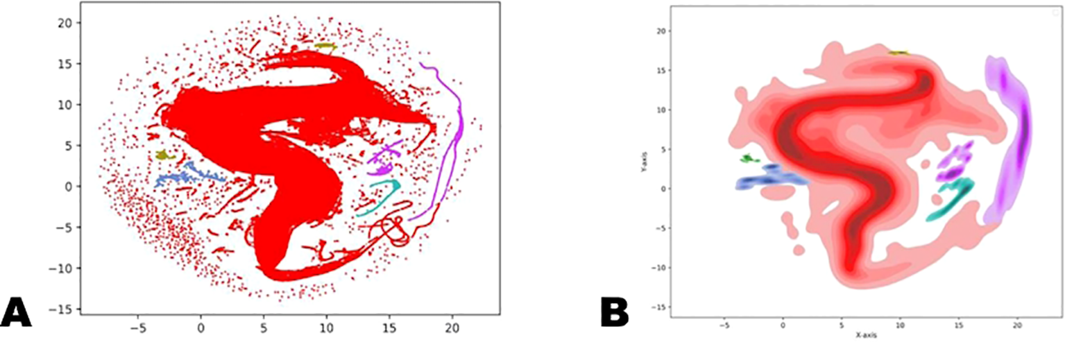
(a, b) Clustering using the DBSCAN method on the full data set with class densities on the full dataset in embedding vectors space. Visualization via (a) scatter plot; (b) kde-plot (density plot).
As a result, the following clusters were identified (Table 1, the list is incomplete):
Table 1
| Class number | Objects quantity |
|---|---|
| -1 | 295 248 |
| 0 | 187 245 |
| 50 | 9 454 |
| 65 | 3 133 |
| … | |
| 90 | 5 |
Number of objects assigned to each class using DBSCAN on whole photographs.
The main array of vectors (i.e., “points” on this graph) is clearly identified by the model, corresponding to class “0” on the graph. On the other hand, the model also detected several smaller classes, recognizing them separately from the “scatter” of outliers (in DBSCAN, outliers are typically assigned the class “-1”). The primary class “0” and the outlier class “-1” (together accounting for almost 95% of the points) are clearly visible, along with numerous smaller classes.
Of particular interest is the third-largest connected class, numbered “50”. Visual inspection of the data corresponding to the vectors in this class reveals that it contains the main set of dark images. Examples of photographs from the class numbered “50” are shown in Figures 4a, b.
Figure 4
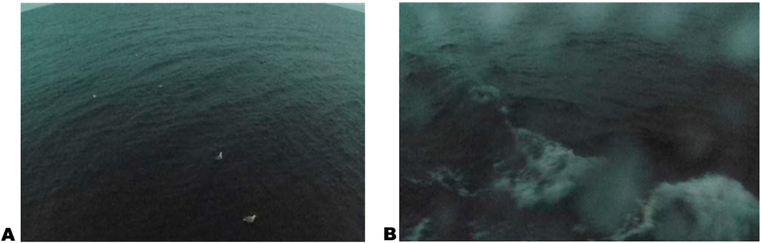
(a, b) Two examples of frames taken at night and recognized as “anomaly” objects (by us), as they belong to the minor class separate from the main one. They were excluded from further analysis because of low light.
These images were excluded from the dataset, as they were considered as outliers. Thus, the model demonstrated that at the top level it is able to recognize the most significant features in data objects. Invalid nighttime photos determined in this way (not manually) were removed from the dataset, and we did the main work with ordinary daytime photos.
2.4 Anomaly labelling
Having completed preliminary data processing and outlier image removal, the next task involves detecting anomalies directly within images. This requires supervised learning and consequently manual annotation of objects in photographs. This data markup also serves to measure average object sizes for each dataset class. In determining image anomalies, we considered not only object appearance but also their presence or absence in adjacent frames and their location. White objects of unknown origin appear frequently in frames—it cannot be definitively determined whether these are surface reflections, wave foam, or actual marine pollution objects. Additionally, water droplets occasionally land on the camera lens, causing image blurring.
Video frame color characteristics depend significantly on time of day, with notable changes in visible sea surface and sky shades. Frames from the same video are most similar to each other, but even then, water surface color can vary greatly, from blue-green to bright blue.
For annotation, every 50th frame from the dataset was used. Annotating all 511,262 frames would be too labor-intensive for this study; meanwhile, we needed representative data from the entire expedition, not just initial days.
Approximately 10,000 photographs were annotated using the LabelStudio application. The annotation data was subsequently analyzed using pandas (a Python library for data manipulation and analysis).
We decided to search for and label the following anomaly types: Birds (Example in Figure 5a), Marine Litter (Example in Figure 5b), Glares, and Droplets on the camera.
Figure 5
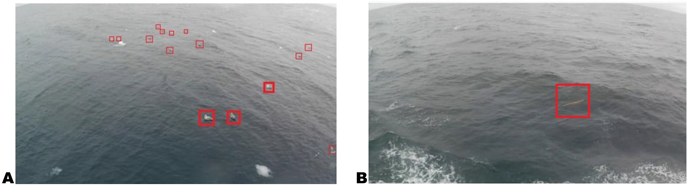
(a, b) Examples of images containing anomalies of various types. (a) contains examples of identified birds, (b) shows an example of marine litter.
These anomaly types were chosen for several reasons. Detecting litter constitutes the study’s primary goal. Birds appear similar to each other and occur regularly, making it interesting to analyze whether the model can recognize their similarity and classify them into a separate class. Colorful glares are of interest due to their distinct contrast with the standard appearance of sky and water surface. Water droplets on the camera were annotated to later analyze the problem of corrupted frames due to blurring of entire images or their parts. A total of 10,064 photos from the full dataset were labeled, including:
-
2,716 “Bird” objects among 559 pictures.
-
56 “Marine Litter” objects among 54 pictures.
-
18,400 “Droplet” objects among 3,709 pictures.
-
1,737 “Glare” objects among 969 pictures.
We observed that a large number of birds were found, often appearing in groups. As expected, litter seldom appears in images and generally occurs as solitary objects. Water droplets occur very frequently and are often present in large quantities within single images, typically appearing in successive frame groups. Droplets and birds simultaneously appear in 167 images, while droplets and litter appear together in 18 images. It might be worthwhile to consider mounting the camera higher or using a camera with a wiper. Glares also occur regularly, most frequently as bright reflections of sunsets or sunrises.
To summarize the preliminary data processing: initially, there were over 500,000 “raw” data photographs. However, we first identified the set of irrelevant dark images taken at night, then selected every 50th frame from the resulting dataset to optimize calculations and better utilize computational resources. Consequently, the actual dataset volume for most subsequent manipulations comprised approximately 10,000 images. Henceforth, the term “dataset” refers to this reduced set.
The aforementioned labelled images consisting of 10000 frames with text information about object bounding boxes are also published on Kaggle within “Marine monitoring, autumn 2023, Dalnie Zelentsy” dataset (Jeong et al., 2024).
3 Results
3.1 Data exploration based on small fragments of images
In this part of our research, we conduct analysis on data from the already prepared working dataset. Here, we combine the neural network with MoCo approach on small fragments of each image with a CatBoost classifier (Prokhorenkova et al., 2018) trained to recognize specific classes.
Thus, while we continue utilizing the MoCo approach for unsupervised anomaly detection, in this scenario, a supervised learning model based on the CatBoost framework will be used separately for classification.
3.1.1 Data fragmentation
This training aimed to validate the model’s anomaly detection capabilities and optimization through loss function minimization. Previous ResNet50+MoCo experiments successfully identified large-scale anomalies (nighttime dark frames) but failed to detect fine-grained image details. To address this limitation, we implemented image fragmentation—sampling small fragments from existing images—to enable detection of small details that would otherwise be overlooked.
The fragmentation process employed fixed square crops of 120×120 pixels, determined from average object sizes in annotated “litter” and “birds” classes. A pseudorandom generator selected coordinates for the top-left corner of each cropping rectangle, after which all fragments were resized to uniform dimensions through scaling.
We divided the task into two approaches using different loss functions and data sampling methods within MoCo training. The BCE-based approach uses Binary Cross-Entropy loss with explicitly defined positive and negative pairs, while the InfoNCE-based approach uses InfoNCE loss where only positive pairs are explicitly defined and all non-positive pairs serve as negatives.
Positive pairs were defined identically for both approaches as two fragments from the same image with inter-fragment distance between 0.2 and 1.0 fragment lengths, preventing excessive overlap while maintaining similarity. For negative pairs, the BCE approach considered fragments from images at least 10 frames apart (corresponding to 10-second temporal separation), while the InfoNCE approach automatically classified all non-positive pairs as negative. Both approaches used identical fragmentation algorithms and trained ResNet50+MoCo networks for 100 epochs.
3.1.2 Data structure and data visualization
Previously, in the preliminary dataset processing, we only applied the MoCo approach to identify nighttime images. At that time, images were not divided into individual fragments; instead, the entire image was used, compressed by a factor of 10 in both dimensions.
The logic for selecting positive and negative pairs has also changed. Now, a positive pair consists only of two fragments from the same photo, with a distance between them no more than one length of the reference fragment but at least 0.2 lengths (which equals to 120 pixels). This condition was introduced to avoid excessive overlapping and matching between fragments. The same logic for selecting positive pairs was used in both the BCE-based approach (with binary classification) and the InfoNCE-based approach (only with positive pairs). Figures 6a, b show two pairs of images, examples of both positive and negative pairs taken from the dataset of fragments.
Figure 6
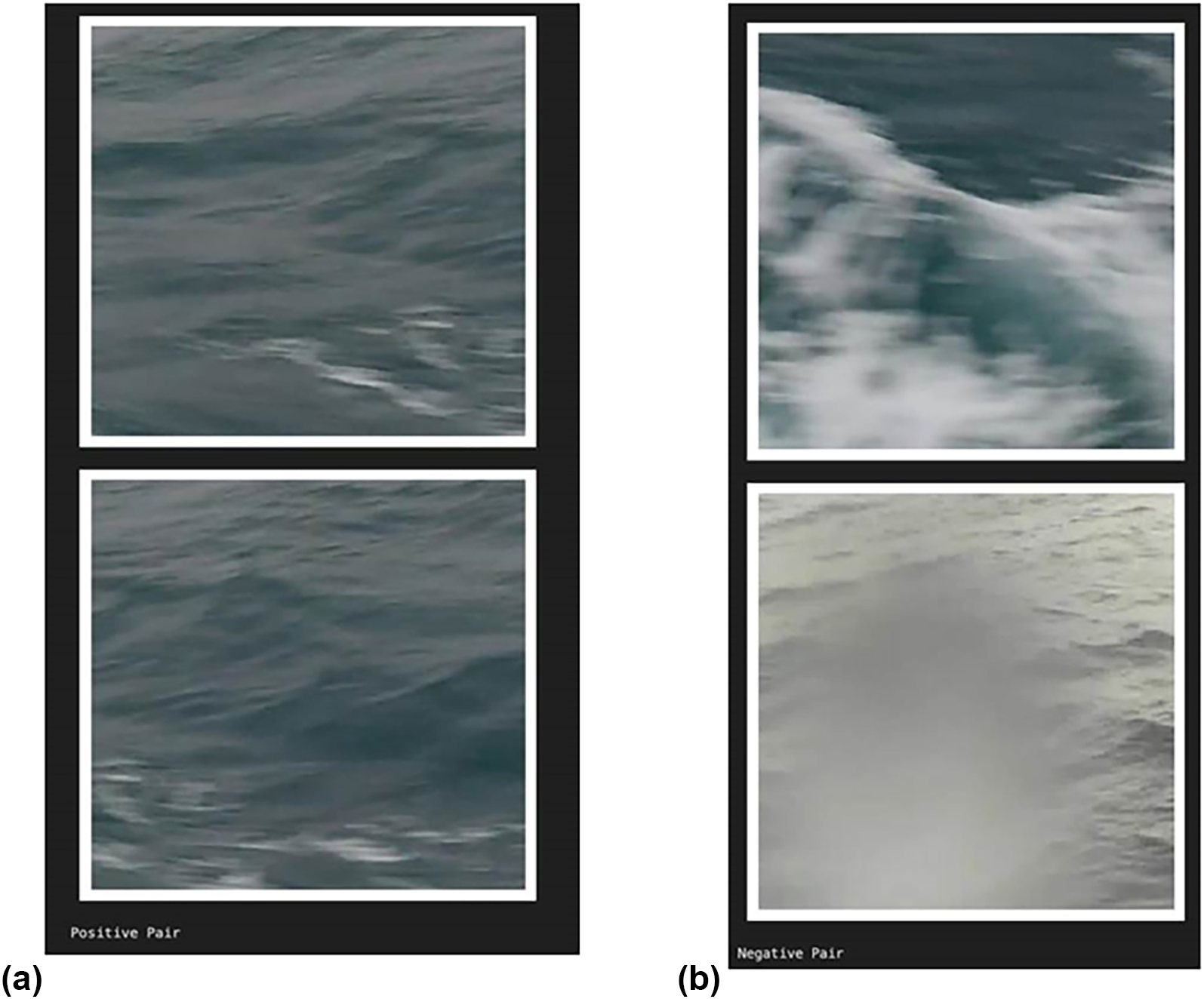
(a, b) An example of a positive pair of data objects (fragments). An example of (a) positive and (b) negative pair of data objects (fragments).
To ensure the correct functioning of the algorithm during training and the accuracy of detecting positive and negative pairs, it was decided to verify how different the hidden representation vectors are for fragments created using the pair generation algorithm from the previous section, which we know to be either:
-
markedly different, or
-
highly similar.
Cosine similarity was used for comparison, which was calculated for each pair of fragments on the hidden representation vectors computed by the neural network encoder. Cosine similarity is a measure of similarity between two vectors, which can be represented using the dot product and the norm (Equation 5):
The choice of this similarity measure is justified by its high accuracy with high-dimensional data. In our case, the dimensionality of the hidden representation vectors is 256.
After we fully defined our fragmentation technique, we launched training of the ResNet50 network with MoCo approach on all fragments of our photographs, of which there are approximately 5.8 million objects. The total duration of this ML training task was 500 epochs; a single GPU (NVIDIA GeForce RTX 4090) was used.
In order to track how progressively well in distinguishing positive pairs from negative ones our model is emerging, we monitored the cosine distribution of said pairs on the initial 10 epochs. Figures 7a, b compare the distribution graphs of cosine similarity for positive and negative pairs at the start of training (after the 0th epoch) and after completing several training epochs (after the 9th epoch) given the BCE-based learning approach is used (i.e., the one with the BCE loss function). Positive and negative pairs are highlighted in different colors for the sake of clarity.
Figure 7
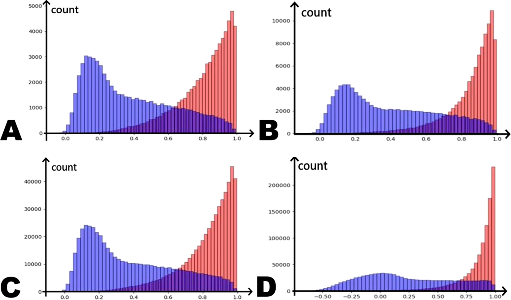
Distribution of cosine distances between positive (red) and negative (blue) fragment pairs: (a) BCE-based approach after 0th epoch; (b) BCE-based approach after 9th epoch; (c) InfoNCE-based approach after 0th epoch; (d) InfoNCE-based approach after 9th epoch.
Figures 7c, d show similar distributions after the 0th and 9th epochs in the InfoNCE-based approach.
It is quite apparent that the InfoNCE-based approach in this context yields more distinct results—the distance between the peaks of the distribution for negative and positive pairs increases more rapidly, and the overlap region decreases as well. This may indicate that using InfoNCE-based approach could produce better results.
After completing the training of the model in both scenarios, the obtained feature vectors were visualized on the graph. Since the dimension of the output vector of hidden representations obtained as a result of training and using a neural network is 256, it is necessary to reduce the number of dimensions to 2 in order to obtain an understandable visualization of hidden representation vectors in a two-dimensional space. The UMAP dimension reduction method was used, a brief description of which is given in Section 2.2.4.
Figures 8 , 9a–e present the results of this visualization. In an ideal scenario, we expect the model to be able to separate feature vectors from different classes significantly far apart, but in practice, overlaps between classes are inevitable. Therefore, the fewer such overlaps, the better the model has performed in clustering and classifying the data.
Figure 8
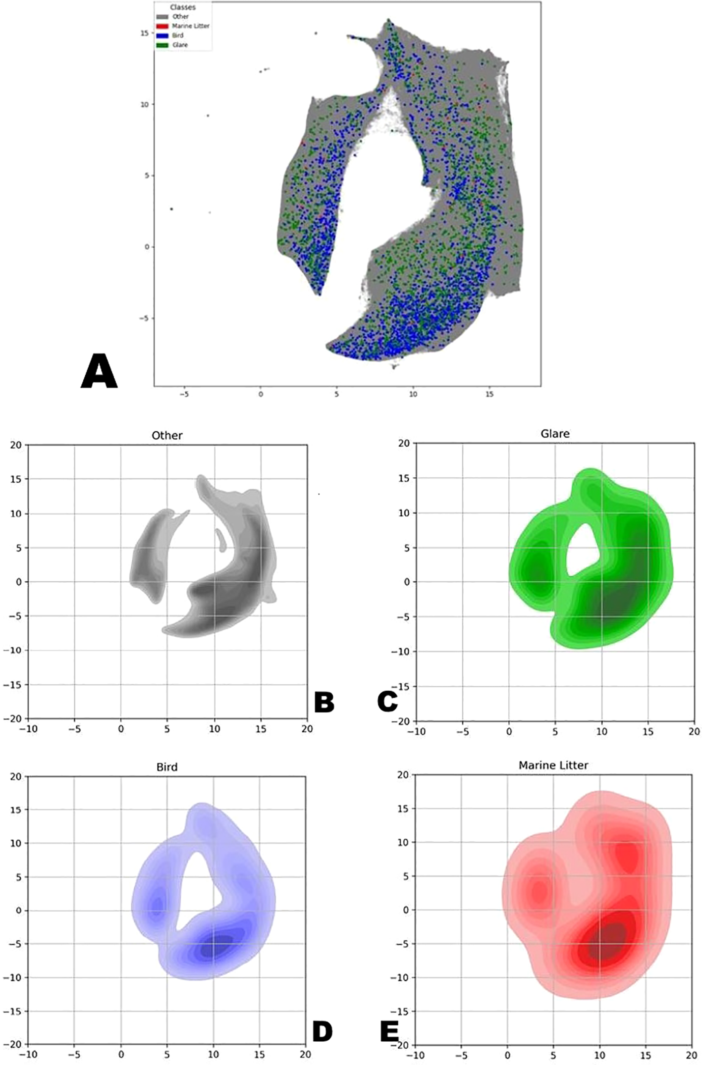
(a) Two-dimensional representation of hidden representation vectors obtained by the UMAP method on a marked-up data set. BCE-based learning approach. (b-e) A two-dimensional representation of the density of the distribution of vectors from UMAP, similar to the previous figure, in the context of individual classes: (a) Gray – “empty” and “droplets”, (b) green – “glare”, (c) blue – “birds”, (d) red – “marine litter”. BCE-based learning approach.
Figure 9
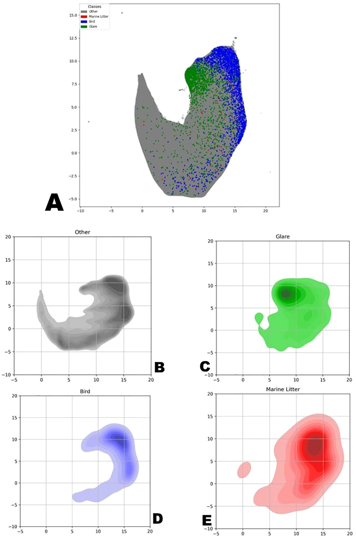
(a) Two-dimensional representation of hidden representation vectors obtained by the UMAP method on a marked-up data set. InfoNCE-based learning approach. (b-e) A two-dimensional representation of the density of the distribution of vectors from UMAP, similar to the previous figure, in the context of individual classes: (a) Gray – “empty” and “droplets”, (b) green – “glare”, (c) blue – “birds”, (d) red – “marine litter”. InfoNCE-based learning approach.
Figures 8a–e show the distribution of vectors obtained using BCE-based approach with the UMAP method—first an overall view with all vectors, followed by individual visualizations for each class. Figure 8 a) shows the full picture with classes combined; b) gray dots for droplets and unmarked objects; c) green dots for “glare” anomalies; d) blue dots for “bird” anomalies; e) red dots for “marine litter” anomalies.
Figures 9a-e are analogous to Figures 8a-e, but they depict distributions acquired using InfoNCE-based learning approach.
One may note that the overlap between the classes, although not very large, still can be noticed visually, both on the scatter plot and on the density plots. Despite this, a positive outcome of the neural network’s performance can still be observed—by comparing the density distribution graphs of vectors across all classes, constructed in the same coordinates, it’s noticeable that the areas of the major concentration of vectors are located in different parts of the graph.
One may also draw one more conclusion as a result of dimensionality reduction with UMAP that this method delivers is suitable for relatively fast computations given limited computational resources, and it is also capable of processing the entire dataset consisting of 5769792 vector examples.
Among the two approaches we tested, BCE-based training demonstrates slightly less overlap between the classes compared to the results of the neural network trained with InfoNCE loss function.
3.1.3 Classification of small fragments of sea surface imagery
Classification was conducted using CatBoost algorithms (see Section 2.2.3 for a brief description) employing hidden representation vectors. These vectors were obtained by training a ResNet50 network within the MoCo approach (see Section 2.2.1) with two different parameter sets: the BCE-based learning approach with both positive and negative pairs specified, and the InfoNCE-based learning approach. As mentioned above in the sections on fragmentation and data structure visualization, we are not working with the original image array, but with a new dataset that represents all the 120x120 pixel fragments obtained from these original images. This new “large” secondary dataset of image fragments (about 5.8 million items) was divided into training and validating subsets by ratio 70:30 – randomly selected 70% of the fragments were used for training, while remaining 30% were left for the validation.
The CatBoost classifier for each approach was run multiple times—once using an unbalanced dataset and several times with datasets of various balance ratios. The balancing terms refer to the following: among nearly 6 million objects in the dataset (since each of approximately 10,000 images is divided into 576 square fragments without overlap), only about 4,500 are labeled as “Marine Litter,” “Bird,” or “Glare” (“Droplets” were ultimately excluded from consideration in this task), making the raw unbalanced dataset poorly suited for effective supervised model training. On average, one relevant data object (either “Marine Litter,” “Bird,” or “Glare” class) in the raw unbalanced dataset would appear less frequently than 1 in 1,000.
Therefore, the term “balanced” refers to all derivative datasets where this ratio is adjusted. Five datasets were used in total: dataset No. 1 was the original unbalanced one, then datasets No. 2, 3, 4, and 5 were various versions of the balanced dataset where the proportion of non-anomalies to the total number amounts to 10%, 1%, 0.1%, and 0.05%, respectively. The ratio of non-anomalous data (i.e., vectors of class 0) to the rest in each of these five cases is as follows:
-
5.8 × 10⁶ “empty” ones to 4.2 × 10³ points with relevant data (approximately 0.07% or 1 to 1,400).
-
5.8 × 10⁵ to 4.2 × 10³ – 0.7% or 1 to 140.
-
5.8 × 10⁴ to 4.2 × 10³ – 7% or 1 to 14.
-
5.8 × 10³ to 4.2 × 10³ – 70% or 1 to 1.4.
-
2.8 × 10³ to 4.2 × 10³ – here, labeled objects outnumber the others; the ratio is 150% or 3 to 2.
The following parameter values for CatBoost were used (Table 2):
Table 2
| Parameter | Value |
|---|---|
| iterations | 1000 |
| depth | 12 |
| leaf_estimation_iterations | 10 |
| learning_rate | 0.0001 |
| loss_function | MultiClass |
| eval_metric | TotalF1 |
| class_weights | The best weights were set using the Optuna optimizer |
Number of objects assigned to each class using DBSCAN on whole photographs.
For ease of data interpretation, Figures 10a–c show the F1-score value progression depending on the ratio of “non-anomalous” to “anomalous” objects, or in other words, depending on the dataset number, for all classes average (a), for “Birds” class (b), and for “Glare” class (c), respectively. To recall, in the current notation, dataset No. 1 is unbalanced (taken as-is), while in dataset No. 5, the ratio of anomalies to non-anomalies is at its maximum.
Figure 10
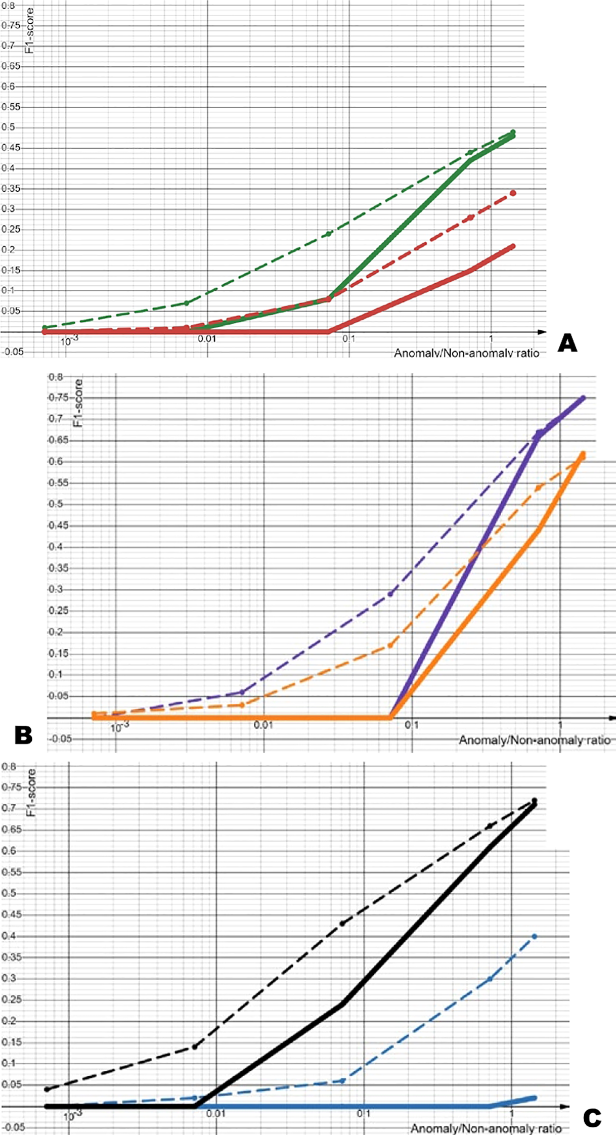
(a-c) Logarithmic graphs of average F1-scores: (a) all three classes with BCE-based (red) and InfoNCE-based (green) approaches; (b) class 2 “Birds” with BCE-based (orange) and InfoNCE-based (purple) approaches; (c) class 3 “Glare” with BCE-based (blue) and InfoNCE-based (black) approaches. Solid lines represent calculations without class weights, dashed lines with weights.
Each experiment was then conducted on two different trained hidden representation vectors: from the BCE-based approach and the InfoNCE-based learning approach, respectively.
Following this, each experiment was carried out in two modes: one employing class weight optimization and the other using default class weights equal to 1. Here, the Optuna hyperparameter optimization framework (Akiba et al., 2019) was exploited for algorithmically searching for the best class weight values under the condition of maximizing the F1-score metric.
4 Conclusion
This study addressed the critical challenge of automating marine litter monitoring, specifically targeting the bottleneck created by the dependency on large, manually annotated datasets required by most supervised AI models. We successfully developed and evaluated a novel anomaly detection framework capable of identifying floating marine litter from sea surface imagery using primarily unlabeled data. Our main contribution is the demonstration that a contrastive learning approach, combined with a unique sampling strategy based on the ergodic properties of the sea surface, provides a viable pathway for scalable and cost-effective monitoring.
In fulfillment of our research objectives, we have achieved the following. Firstly, we developed a robust method for anomaly detection using a ResNet50 model trained within the Momentum Contrast (MoCo) framework. This approach successfully learned to distinguish atypical visual patterns (anomalies) from the homogenous texture of the sea surface without prior knowledge of what constitutes “litter”.
Secondly, we proposed and implemented a novel data sampling strategy that leverages the spatial autocorrelation of sea wave fields. This technique proved effective for generating the vast number of positive and negative pairs required for contrastive learning from raw, unlabeled video footage, which is a key methodological advance.
Lastly, our evaluation on a large, real-world dataset of over 500,000 images (and 10’000 annotated into 4 different categories) demonstrated the model’s capability to identify various anomalies. The system achieved a high F1-score of up to 0.75 in detecting birds, confirming its effectiveness as an anomaly detector. However, its performance on the primary target class—marine litter—was less distinct, highlighting a key challenge related to the subtlety and variability of litter objects compared to more prominent anomalies.
Another important conclusion is that training model quality metrics heavily depend on the quantity, quality, and configuration of input data. To achieve acceptable results, it is necessary to enhance samples containing data objects useful for training among predominantly featureless data (i.e., make them appear more frequently).
We continue our research on a dataset of marine images divided into fragments. Research has been conducted using a convolutional neural network trained with the MoCo approach and CatBoost, optimizing the F1-score metric averaged across all classes. Since among the three classes identified, the model shows the best results not on floating marine litter but on other classes, future research should focus on maximizing the F1 indicator specifically for marine litter detection. Since the InfoNCE-based learning approach (using the InfoNCE loss function with negative pairs defined as non-positive) achieves higher object identification quality relative to the F1-score in the current work, it is advisable to use only this approach in subsequent tasks.
Additionally, it is worthwhile to explore other approaches in greater detail, and one of the most obvious choices would be using YOLO networks. Here, it is similarly worth considering both detecting all three anomaly types (marine litter, birds, glares) and training the model solely for marine litter detection.
Statements
Data availability statement
The datasets presented in this study can be found in online repositories. The names of the repository/repositories and accession number(s) can be found below: https://doi.org/10.34740/KAGGLE/DSV/12199049.
Author contributions
OB: Writing – original draft, Writing – review & editing. MK: Writing – review & editing.
Funding
The author(s) declare that financial support was received for the research and/or publication of this article. This research was carried out under the Agreement No. 075-03-2025-662 dated January 17, 2025.
Acknowledgments
We thank Maria Pogojeva (MSU Faculty of Geography, Moscow), Viktoria Spirina (N. N. Zubov State Oceanographic Institute, Moscow), and Polina Krivoshlyk (Shirshov Institute of Oceanology, Moscow) for collecting and providing the observational records and source video data from the marine expedition, as well as for supplying details on the equipment installation and operating regimes.
Conflict of interest
The authors declare that the research was conducted in the absence of any commercial or financial relationships that could be construed as a potential conflict of interest.
Generative AI statement
The author(s) declare that no Generative AI was used in the creation of this manuscript.
Any alternative text (alt text) provided alongside figures in this article has been generated by Frontiers with the support of artificial intelligence and reasonable efforts have been made to ensure accuracy, including review by the authors wherever possible. If you identify any issues, please contact us.
Publisher’s note
All claims expressed in this article are solely those of the authors and do not necessarily represent those of their affiliated organizations, or those of the publisher, the editors and the reviewers. Any product that may be evaluated in this article, or claim that may be made by its manufacturer, is not guaranteed or endorsed by the publisher.
References
1
Akiba T. Sano S. Yanase T. Ohta T. Koyama M. (2019). “ Optuna: a next-generation hyperparameter optimization framework. The 25th ACM SIGKDD International Conference on Knowledge Discovery & Data Mining, 2623–2631.
2
Aliani S. Molcard A. (2003). Hitch-hiking on floating marine debris: macrobenthic species in the western Mediterranean Sea. Hydrobiologia503, 59–67. doi: 10.1023/B:HYDR.0000008630.90632.1a
3
Andrady A. L. (2015). “ Persistence of plastic litter in the oceans,” in Marine anthropogenic litter (Cham, Switzerland: Springer), 57–72.
4
Bilousova O. Krivoshlyk P. Spirina V. Krinitskiy M. Pogojeva M. (2025). Marine monitoring, autumn 2023 (Dalnie Zelentsy: Kaggle). doi: 10.34740/KAGGLE/DSV/12199049
5
Boerger C. M. Lattin G. L. Moore S. L. Moore C. J. (2010). Plastic ingestion by planktivorous fishes in the North Pacific Central Gyre. Mar. pollut. Bull.60, 2275–2278. doi: 10.1016/j.marpolbul.2010.08.007
6
Derraik J. G. B. (2002). The pollution of the marine environment by plastic debris: a review. Mar. pollut. Bull.44, 842–852. doi: 10.1016/S0025-326X(02)00220-5
7
de Vries R. (2022). Using AI to monitor plastic density in the ocean. The Ocean Clean Up Project. Available online at: www.theoceancleanup.com (Accessed October 12, 2025).
8
Ershova A. Vorotnichenko E. Gordeeva S. Ruzhnikova N. Trofimova A. (2024). Beach litter composition, distribution patterns and annual budgets on Novaya Zemlya archipelago, Russian Arctic. Mar. pollut. Bull.204, 116517. doi: 10.1016/j.marpolbul.2024.116517
9
Ester M. Kriegel H.-P. Sander J. Xu X. (1996). “ A density-based algorithm for discovering clusters in large spatial databases with noise,” in AAAI Press, Proceedings of the 2nd International Conference on Knowledge Discovery and Data Mining (KDD-96). 226–231.
10
Galgani F. Hanke G. Maes T. (2015). “ Global distribution, composition and abundance of marine litter,” in Marine anthropogenic litter. Eds. BergmannM.GutowL.KlagesM. (Cham, Switzerland: Springer), 29–56.
11
Galgani F. Pastor R. O. S. Ronchi F. Tallec K. Fischer E. Matiddi M. et al . (2023). Guidance on the monitoring of marine litter in European seas – an update to improve the harmonised monitoring of marine litter under the Marine Strategy Framework Directive (Luxembourg: Publications Office of the European Union).
12
Gall S. C. Thompson R. C. (2015). The impact of debris on marine life. Mar. pollut. Bull.92, 170–179. doi: 10.1016/j.marpolbul.2014.12.041
13
Garcia-Garin O. Borrell A. Aguilar A. Cardona L. Vighi M. (2020). Floating marine macro-litter in the North Western Mediterranean Sea: results from a combined monitoring approach. Mar. pollut. Bull.159, 111467. doi: 10.1016/j.marpolbul.2020.111467
14
González-Fernández D. Hanke G. Pogojeva M. Machitadze N. Kotelnikova Y. Tretiak I. et al . (2022). Floating marine macro litter in the Black Sea: toward baselines for large scale assessment. Environ. pollut.309, 119816. doi: 10.1016/j.envpol.2022.119816
15
Gayathrri K. Dash S. K. Usha T. Thanabalan P. Nimalan K. Mayamanikandan T. et al . (2025). Marine litter assessment using remote sensing techniques - a review. Curr. Sci.129, 118–128. doi: 10.18520/cs/v129/i2/118-128
16
He K. Fan H. Wu Y. Xie S. Girshick R. (2020). Momentum contrast for unsupervised visual representation learning. arXiv. preprint. arXiv:1911.05722.
17
Jeong Y. Shin J. Lee J.-S. Baek J.-Y. Schläpfer D. Kim S.-Y. et al . (2024). A study on the monitoring of floating marine macro-litter using a multi-spectral sensor and classification based on deep learning. Remote Sens.16. doi: 10.3389/rs16234347
18
Kako S. Kataoka T. Matsuoka D. Takahashi Y. Hidaka M. Aliani S. et al . (2025). Remote sensing and image analysis of macro-plastic litter: a review. Mar. pollut. Bull.222, 118630. doi: 10.1016/j.marpolbul.2025.118630
19
Katsanevakis S. (2014). Marine debris, a growing problem: sources, distribution, composition, and impacts. Open Access Library. J.1, e773. doi: 10.4236/oalib.1100773
20
Kylili K. Hadjistassou C. Artusi A. (2021). An intelligent way for discerning plastics at the shorelines and the seas. Environ. Sci. pollut. Res.27, 42631–42645. doi: 10.1007/s11356-020-09855-y
21
Lebreton L. Slat B. Ferrari F. Sainte-Rose B. Aitken J. Marthouse R. et al . (2018). Evidence that the Great Pacific Garbage Patch is rapidly accumulating plastic. Sci. Rep.8, 4666. doi: 10.1038/s41598-018-22939-w
22
Lippiatt S. Opfer S. Arthur C. (2013). Marine debris monitoring and assessment: recommendations for monitoring debris trends in the marine environment. NOAA Technical Memorandum NOS-OR&R-46 (Silver Spring, MD: NOAA Marine Debris Program (National Oceanic and Atmospheric Administration)).
23
McInnes L. Healy J. (2018). UMAP: uniform manifold approximation and projection for dimension reduction. arXiv. preprint. arXiv:1802.03426. 3, 861. doi: 10.21105/joss.00861
24
Pogojeva M. Yakushev E. Terskii P. Glazov D. Aliautdinov V. Korshenko A. et al . (2021). Assessment of Barents Sea floating marine macro litter pollution during the vessel survey in 2019. Tomsk. State. Pedagogical. Univ. Bull.332, 87–96.
25
Prakash N. Zielinski O. (2025). AI-enhanced real-time monitoring of marine pollution: part 1 - a state-of-the-art and scoping review. Front. Mar. Sci.12. doi: 10.3389/fmars.2025.1486615
26
Prokhorenkova L. Gusev G. Vorobev A. Dorogush A. V. Gulin A. (2018). CatBoost: gradient boosting with categorical features support. arXiv. preprint. arXiv:1810.11363.
27
Raju M. P. Veerasingam S. Suneel V. Asim F. S. Khalil H. A. Chatting M. et al . (2025). A machine learning-based detection, classification, and quantification of marine litter along the central east coast of India. Front. Mar. Sci.12. doi: 10.3389/fmars.2025.1604055
28
Srinivasa R. M. (2025). Hybrid deep learning approach for marine debris detection in satellite imagery using UNet with ResNext50 backbone. J. Appl. Sci. Technol. Trends6, 50–60. doi: 10.38094/jastt61243
29
Topouzelis K. Papageorgiou D. Suaria G. Aliani S. (2021). Floating marine litter detection algorithms and techniques using optical remote sensing data: a review. Mar. pollut. Bull.170, 112675. doi: 10.1016/j.marpolbul.2021.112675
30
Veettil K. Bijeesh Nguyen H.-Q. Hauser L. Doan D. Quang N. (2022). Coastal and marine plastic litter monitoring using remote sensing: a review. Estuar. Coast. Shelf. Sci.279, 108160. doi: 10.1016/j.ecss.2022.108160
31
Watanabe J. I. Shao Y. Miura N. (2019). Underwater and airborne monitoring of marine ecosystems and debris. J. Appl. Remote Sens.13, 14522. doi: 10.1117/1.JRS.13.014522
32
Xue B. Huang B. Chen G. Li H. Wei W. (2021). Deep-sea debris identification using deep convolutional neural networks. IEEE J. Sel. Topics. Appl. Earth Observ. Remote Sens.14, 8909–8921. doi: 10.1109/JSTARS.2021.3109968
Summary
Keywords
floating marine litter, marine environment monitoring, artificial intelligence, machine learning, artificial neural networks, data structure exploration
Citation
Bilousova O and Krinitskiy M (2025) Exploratory data analysis of visual sea surface imagery using machine learning. Front. Mar. Sci. 12:1689783. doi: 10.3389/fmars.2025.1689783
Received
20 August 2025
Revised
16 November 2025
Accepted
18 November 2025
Published
11 December 2025
Volume
12 - 2025
Edited by
Takafumi Hirata, Hokkaido University, Japan
Reviewed by
Mustapha Aksissou, Abdelmalek Essaadi University, Morocco
Ana Carolina Luz, Instituto de Estudos do Mar Almirante Paulo Moreira, Brazil
Updates
Copyright
© 2025 Bilousova and Krinitskiy.
This is an open-access article distributed under the terms of the Creative Commons Attribution License (CC BY). The use, distribution or reproduction in other forums is permitted, provided the original author(s) and the copyright owner(s) are credited and that the original publication in this journal is cited, in accordance with accepted academic practice. No use, distribution or reproduction is permitted which does not comply with these terms.
*Correspondence: Olga Bilousova, belousova.o@phystech.edu
Disclaimer
All claims expressed in this article are solely those of the authors and do not necessarily represent those of their affiliated organizations, or those of the publisher, the editors and the reviewers. Any product that may be evaluated in this article or claim that may be made by its manufacturer is not guaranteed or endorsed by the publisher.