Abstract
Considering the complex offshore environment, where small robotic fish are exposed to surface disturbances from wave forces, suspended particles, and model uncertainties, as well as deep-water disturbances from bottom currents, this paper proposes an inverse sliding mode control strategy based on a disturbance observer to enhance trajectory tracking robustness. The research focuses on a tail-fin-driven bionic robotic fish. Utilizing its kinematic and dynamic models, a virtual control law based on an agent dynamics model is proposed, with the tail fin integrated as a real control input. A nonlinear disturbance observer with controllable convergence characteristics is developed to estimate and compensate for disturbances, including wave forces and model uncertainties. Additionally, a velocity error correction function is introduced to mitigate the impact of strong disturbances. Based on Lyapunov theory, an adaptive sliding mode control law is derived to ensure system stability. The control law for the caudal fin swing angle and bias is obtained by inverting the virtual control inputs, applied to the robotic fish’s accurate model. Numerical simulations show that the disturbance observer’s tracking error remains below 5%, and the trajectory tracking error is within 0.1 meters, representing only 2.2% of the robotic fish’s body length. Compared to mainstream control methods, the proposed approach significantly enhances robustness in contrast to the conventional sliding mode control with observers, and exhibits substantially smaller tracking errors, especially during trajectory transitions.
1 Introduction
In recent years, as the global energy structure transforms and marine resource development deepens, the strategic value of marine energy has become more prominent (Li M. et al., 2025; Rehman et al., 2023). The complexity and significance of exploration tasks, such as marine environmental monitoring, resource exploration, and seabed mapping, are steadily increasing. This raises higher demands for the performance of underwater exploration equipment and stimulates widespread interest and enthusiasm among researchers.
Breakthrough progress has been made in current underwater tasks, resulting in a wealth of research achievements. Examples include Visual-textual Fusion Empowered Underwater Image Enhancement (Wang H. et al., 2026), underwater scene clarity reconstruction via multilayer information fusion and self-organized stitching (Wang H. et al., 2024), and Underwater Image Captioning AquaSketch (Li H. et al., 2025). However, Traditional underwater unmanned vehicles typically use propeller propulsion systems driven by hydraulic or electromagnetic principles. Although this mechanical propulsion is well-established in engineering applications, it has significant limitations in energy efficiency, environmental friendliness, and stealth, which hinder its effectiveness for underwater operations. With advances in robotics and bionics research, particularly in the study of efficient propulsion mechanisms in aquatic organisms (e.g., fish BCF movement mode, cephalopod jet propulsion), the development of bionic underwater robots has emerged as a new solution to the limitations of traditional propulsion systems (Ma et al., 2019; Sfakiotakis et al., 1999; Yan et al., 2024). By simulating the flexible deformation of living organisms, vortex control, and other mechanisms, these systems offer significant advantages in propulsion efficiency, maneuverability, and environmental adaptability, representing a key direction for the future of underwater propulsion technology (Nash et al., 2021).
The bionic robotic fish is one of the most iconic underwater robots. The most common bionic fish uses both pectoral and caudal fins in concert for propulsion, with horizontal motion driven either by the caudal fins, a pair of pectoral fins, or a combination of both (Kadiyam and Mohan, 2019). The most common bionic fish tails employ a multilink mechanism with multiple motors working in coordination to drive the fish’s body, enabling oscillation and propulsion. Clapham et al. from Harvard University present a small-scale robotic fish with independent monoarticulated fins, utilizing a binocular fisheye camera for perception and optical communication. This system successfully replicates and interprets autonomous behaviors observed in real fish (Clapham and Hu, 2014). Ning Wang et al. simulated the dorso-ventral motion of a dolphin’s caudal fin and found that a variable thickness flexible caudal fin can enhance propulsive performance (Wang N. et al., 2025). Deqiang Wei et al. found through numerical simulation that the flexible tail fin, driven by a magnetic actuator, offers advantages of high speed and compact size, making it suitable for pipeline surveys (Wei et al., 2023). Fengran Xie et al. designed a wire-driven bionic fish tail that swings by alternately pulling ropes on both sides through a turntable. They also built an experimental platform and proposed a pivotal pattern generator capable of producing four characteristic motion patterns (Xie et al., 2019, 2020). Two rigid-body actuators are used to control the tail motion. Numerical simulations reveal that changes in the shape of the robotic fish increase the total drag force, limiting its maximum speed (Vignesh et al., 2024). Qixin Wang et al. proposed a robotic fish with modular adaptive variable-stiffness passive joints, enabling adaptive stiffness variation without the need for an external drive source (Wang Q. et al., 2025). Currently, bionic fish tail designs primarily use multi-motor drives, linkage mechanisms, and linear drives. However, these methods often suffer from complex drive systems, bulky mechanical structures, insufficient swinging precision, and limited motion range, resulting in a poor overall bionic effect. Given that the control strategy developed for a single-joint robotic fish can be theoretically extended to multi-joint configurations, this study focuses on a single-joint structure to facilitate analysis and controller design (Cao et al., 2022).
Despite the variety of mechanical forms of robotic fish, precise trajectory tracking control mechanisms are required to ensure stable following of the desired path. Kim Donghee et al. proposed a three-degree-of-freedom CPG controller to track in-plane motion trajectories, enabling the bionic fish to move along the desired path (Kim et al., 2008). Longxin Lin et al. proposed a Q-learning controller that incorporates supervised neural networks to control the body oscillations of a bionic fish (Lin et al., 2010). Zheping Yan et al. optimized the parameters of the bionic fish tail using the fish body wave equation and penalty function, integrated the pivotal mode generator with the sliding mode controller, and experimentally verified the effectiveness of the proposed SMC-CPG controller and tail structure (Yan et al., 2022). Ming Wang et al. designed an iterative learning controller for a bionic robotic fish and verified its effectiveness through control simulation experiments (Wang et al., 2020). Pengfei Zhang et al. proposed a two-stage nonlinear model predictive solution for orientation-velocity, which is applicable not only to bionic robotic fish but also to other underwater underdriven robots (Zhang et al., 2020). Xiao Yan and Yue Ma proposed a new control method for flexible robotic fish, offering over 10% greater propulsion compared to conventional control methods (Yan and Ma, 2023). Ruilong Wang et al. proposed an algorithm for trajectory tracking and obstacle avoidance of a robotic fish using nonlinear model predictive control, which leverages current state and environmental data to efficiently regulate its motion in a highly agile manner (Wang R. et al., 2023). Ming Wang et al. proposed a discrete linear quadratic regulator optimization strategy based on the particle swarm optimization algorithm and verified its feasibility and effectiveness in tracking complex trajectories (Wang M. et al., 2023). In the complex underwater operating environment, a single control strategy struggles to meet both the accuracy and robustness requirements for trajectory tracking of the robotic fish. As a result, researchers have begun exploring composite control strategies that integrate the advantages of multiple methods.
In order to simultaneously improve system robustness and control precision, an increasing number of studies have explored composite control frameworks that integrate multiple control paradigms. Ming Wang et al. proposed a novel motion control method for robotic fish based on an impulse neural network and a central pattern generator, and verified the effectiveness of this hybrid control approach (Wang M. et al., 2022). Yizhuo Mu et al. dynamically adjusted the objective function of optimal control using a model predictive control method based on multilayer perceptron, effectively overcoming the complexity of kinematic modeling in robotic fish (Mu et al., 2022). Kewei Ning et al. introduced inverse learning for feed-forward neural networks to achieve real-time trajectory control (Ning et al., 2022). South China University of Technology proposed a hybrid control method based on a model predictive decision-making strategy, which significantly reduces computational errors and achieves fast system convergence (Wang K. et al., 2024). Qixin Wang et al. proposed a deep reinforcement learning-based approach for online control of a machine eel with multiple passive structures, enabling control without relying on underlying control models or strategies (Wang Q. et al., 2022). Yu Wang et al. designed a nonlinear model predictive controller with reinforcement learning to track the trajectory of a machine fish and verified the effectiveness of the proposed approach (Wang Y. et al., 2024). Sijie Li et al. proposed a gliding-oscillating-strategy-based backstepping-adaptive control method to attenuate tracking error jitter (Li et al., 2024). Dongfang Li et al. introduced a fast global terminal sliding mode fuzzy controller that considers tangential displacements and employs a fuzzy adaptive approach to address complex uncertainties, improving the error convergence speed and accuracy of the machine fish system (Li D. et al., 2025). The aforementioned methods have significantly contributed to the research on trajectory tracking of robotic fish. However, the unique challenges of offshore environments—characterized by high-velocity currents, sediment-laden waters, and strong external disturbances—significantly limit the direct applicability of existing control approaches to such scenarios.
The main innovations presented in this paper to address the gaps in current research are as follows:
-
In this paper, we decompose the robotic fish dynamics model into an agent model and an exact model, utilizing both in conjunction.
-
Improving the robustness of robotic fish trajectory tracking through a nonlinear disturbance observer and an adaptive inverse sliding mode control strategy with velocity correction.
-
By directly using the oscillation frequency and bias of the caudal fin as control inputs, the influence of environmental disturbances on the robotic fish is effectively attenuated, thereby reducing the adverse effects caused by the nonlinear mapping relationship in highly perturbed environments.
The rest of the paper is organized as follows: Section II presents the exact dynamics model of the robotic fish and the agent model to reduce computational intensity. Section III outlines the design of the nonlinear disturbance observer, the velocity correction method, and the derivation process of the adaptive inverse sliding mode controller. Additionally, the tail fin model is updated, and the control inputs are derived. Simulation experiments and a discussion of the results are provided in Section IV. Finally, Section V offers concluding remarks.
2 Modeling of dynamics
This section explains the problems related to the robotic fish, including the definition of the two coordinate systems, its kinematics, and the dynamic equations. The dynamic model used in this study is derived from the physical robotic fish prototype (Figure 1) through feature extraction and physics-based simplification.
Figure 1
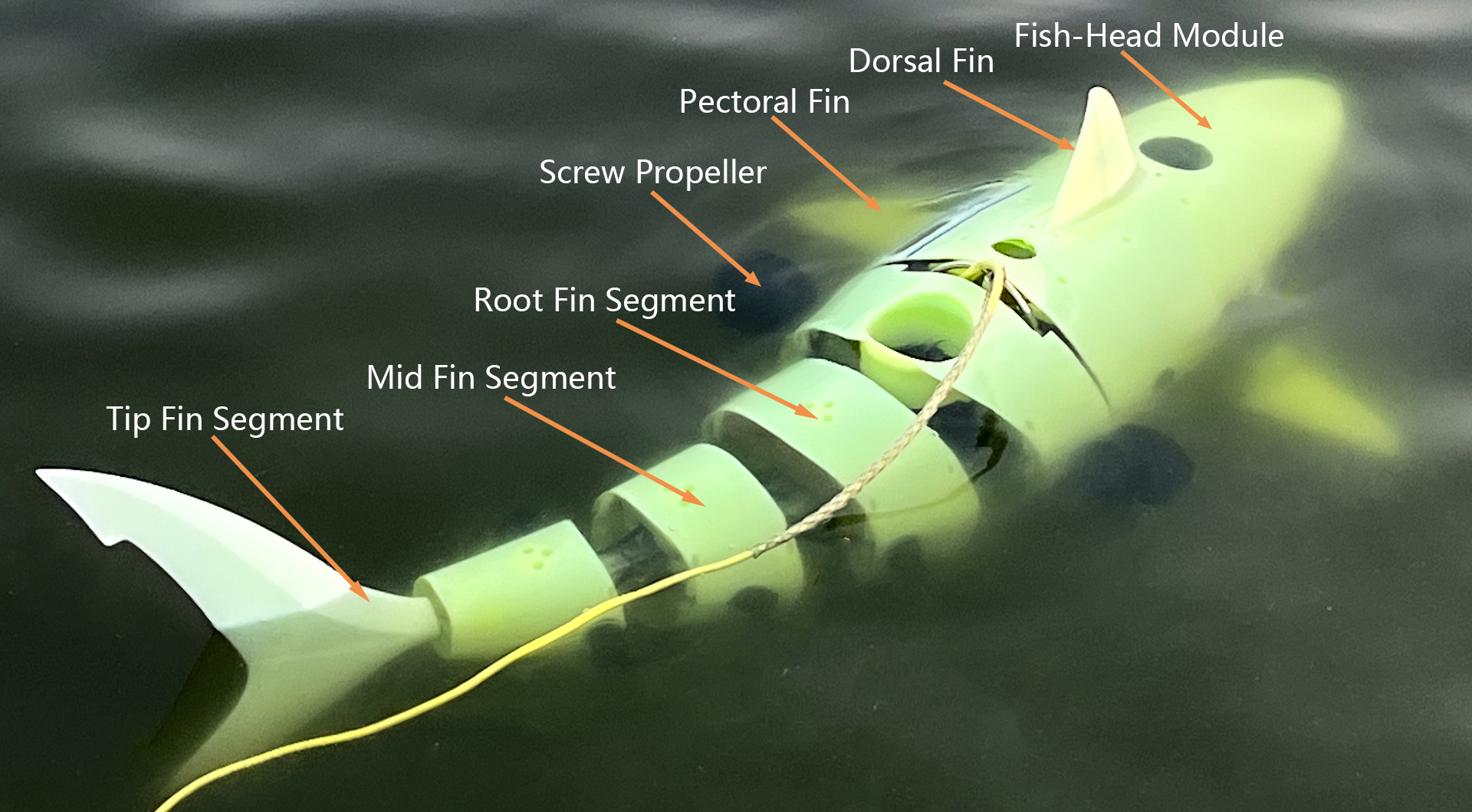
Photograph of the physical robotic fish.
The modeling of the robotic fish is divided into two parts: kinematics and dynamics. To clearly characterize the motion of the robotic fish in the horizontal plane, Figure 2 shows the geometric relationship between the ground-fixed coordinate system {CE} and the body-fixed coordinate system {Cb}.
Figure 2
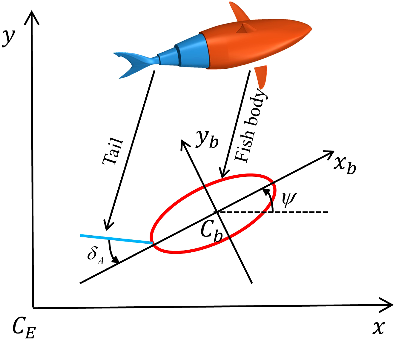
Schematic diagram of robot fish coordinate system.
The horizontal rocking motion, primarily related to the symmetry of the robotic fish, is not considered in the modeling. The kinematic equations of the robotic fish in the horizontal plane are given in Equation 1.
Here x and y denote the positional coordinates of the robotic fish in the Earth’s fixed coordinate system {CE}; denotes the yaw angle; r denotes the yaw angular velocity; and u and v are the forward and traverse velocities, respectively.
In this paper, the higher-order hydrodynamic drag term is neglected, ensuring that the center of gravity of the robotic fish coincides with the center of buoyancy. The exact dynamic equations of the robotic fish are given in Equation 2.
To simplify the computation and facilitate control, a simplified agent model is used as the mathematical model for the controller of the robotic fish. Directly using the exact model in combination with the interference observer and the adaptive inverse sliding mode controller complicates the solution process and poses significant difficulty in inversely solving the caudal fin parameters. The primary focus of this study is not on the detailed derivation of the agent model, but rather on the integrated application of the model with the proposed control strategy. Therefore, this study adopts the well-established underdriven autonomous underwater vehicle (AUV) dynamics model and integrates it with the dynamics modeling of the robotic fish to construct an agent model. By inputting the solved caudal fin parameters into the exact model, the velocity and position of the robotic fish are obtained, completing the control process. The agent model of the robotic fish is given as follows:
where v is the velocity and angular velocity vector in the attached coordinate system; is the inertia matrix; is the composite term of the dynamics model; is the virtual control input; and is the environmental disturbance force and model uncertainty.
3 Controller design
The control objective is to achieve horizontal trajectory tracking of the robotic fish. To address the strong disturbance environment, a nonlinear observer is designed to stabilize the system, even in the presence of significant disturbances. The velocity correction controller is used to reduce the impact of strong disturbances on the motion of the robotic fish; The inverse sliding mode control method is used to derive the virtual control law for the agent model, adapting it to sea currents.
3.1 Nonlinear interference observer design
Under the influence of strong ocean currents, wave-induced forces, and sediment-induced uncertainties, system stabilization is difficult to achieve by solely relying on adaptive sliding mode control to compensate for environmental disturbances. The nonlinear disturbance observer can reduce the steady-state error of the robotic fish by incorporating the external environmental force into measurement or estimation. The nonlinear disturbance observer can inject the external disturbance into the adaptive sliding mode controller as additional signals to enhance the robustness of the system. Given the highly nonlinear nature of the robotic fish’s mathematical model, an exponentially convergent disturbance observer is employed. However, the disturbances measured or estimated are external forces that vary slowly with time but exhibit large peaks.
Let , where is the interference observation and K is the gain parameter of the nonlinear disturbance observer. Define the auxiliary parameter vector as given in Equation 4.
Then, taking the derivative yields Equation 5.
From the machine fish agent model in Equation 3, we obtain the disturbance mathematical model in Equation 6.
Then Equation 7 can be derived.
This, in turn, leads to
By combining Equation 4 and Equation 8, the disturbance observer can be designed as Equation 9.
Which can be further obtained as Equation 10.
Since the targeted disturbance is slowly varying, it can be assumed that , and consequently, the disturbance error is given in Equation 11.
Substituting Equation 10 into the above equation results in
Therefore, rearranging Equation 12, the observation error equation can be expressed as Equation 13.
This resolves to Equation 14.
Since is a constant and , the observer error equation converges, and the convergence accuracy depends on the value of the gain K.
3.2 Velocity correction
In the trajectory tracking problem of a robotic fish, the reference trajectory is directly provided by the navigation system. Let be in the Earth’s fixed coordinate system {CE}, where and are sufficiently smooth functions with at least three derivatives. Since the horizontal motion of the robotic fish in the plane is driven solely by the tail fin, its reference trajectory must satisfy the conditions given in Equation 15.
where is the curvature of the desired trajectory, and is the minimum radius of gyration of the robotic fish.
For control purposes, the position error equation of the robotic fish is expressed as Equation 16.
where and are the trajectory tracking errors of the robotic fish in the body coordinate system {B}; , and are the actual and desired trajectories of the robotic fish in the Earth coordinate system {E}, respectively. The coordinate transformation matrices are non-singular, so the position errors defined in both coordinate systems are equivalent, and their stability is also equivalent. The desired yaw angle of the robotic fish can be directly calculated from the reference trajectory:
Therefore, by means of Equation 17, the tracking error of the yaw angle can be expressed as Equation 18.
The following differential equation for the tracking error is derived by substituting the derivatives of the desired trajectory and yaw angle into the kinematic equations of the robotic fish, as given in Equation 19.
where is t the desired velocity, directly calculated from the desired trajectory of the robotic fish, and its direction is aligned with the straight line connecting the head and tail of the robotic fish, ; is the bow angular velocity, also directly calculated from the desired trajectory of the robotic fish, .
Construct the Lyapunov function for the tracking error of the robotic fish and complete the stability proof for , and .
This can be obtained by taking the derivative with respect to time and substituting Equation 20.
Subsequently, the desired virtual forward speed and angular velocity of the robotic fish are designed based on the above equation. To ensure that the forward speed and angular velocity control inputs correct the tracking error, it is required that these control inputs match the desired virtual forward speed and angular velocity when the positional tracking error , and the bow angle tracking error are zero. The specific expressions are given in Equation 22.
where and are gain coefficients and , .
Substituting and into Equation 21 yields Equation 23.
It can be observed that due to the presence of the nonlinear term , the current system cannot guarantee that remains negative, thus preventing stability in the speed correction system. However, if the longitudinal trajectory tracking error can be reduced to zero or approximately zero, and by appropriately adjusting the gain coefficients and , it is possible to ensure , thereby stabilizing the speed correction system. Therefore, further design of the trajectory tracking controller is required to ensure the overall stability of the control system.
3.3 Adaptive inverse sliding mode control controller design
An adaptive inverse sliding mode controller is designed based on an exponentially converged nonlinear disturbance observer, which compensates for large external disturbances. This controller enables the robotic fish to adjust to real-time current variations in the water, ensuring that these disturbances do not affect the system’s robustness, thereby further reducing the tracking error.
Assumption 1: The value of currents in the robotic fish dynamics model is bounded above and compensated for by the adaptive rate, i.e., .
Assumption 2: The tracking reference trajectory and its derivative, , are both bounded.
Define the trajectory-tracking error as Equation 24.
where represents the actual trajectory of the robotic fish (), and denotes the reference trajectory ().
Then
Constructing Lyapunov functions:
Derivation of the Equation 26, followed by substitution of Equation 25, yields the following result:
Assume , so that the sliding mold surface becomes . It is designed to guide the system state toward the desired dynamic behavior. Among them, introduces the proportional feedback of the position error into the sliding surface. This ensures that if the robotic fish deviates from the target position , the sliding surface will be adjusted to “pull” the system back to the desired trajectory, achieving faster convergence with the help of error feedback.
Let , where is the current adaptive compensation value, and substituting into Equation 27 yields.
Construct a Lyapunov function that integrates position error and sliding surface error:
Differentiating Equation 28 yields Equation 19.
The control law can thus be designed as Equation 30.
It is used to generate the virtual control input (the thrust and torque required by the robotic fish) to drive the system to track the reference trajectory. Where , , are constants and , , , , are current compensation errors.
Then
This part solves the stability problem of the sliding surface, so that if , then . Therefore, continue to construct the Lyapunov function to completely eliminate the influence of the disturbance term.
Here, is the gain constant, and . Differentiating Equation 32 gives Equation 33.
Among them, since the ocean current changes slowly, then .
Substituting Equation 31 gives
The adaptive rate is designed as
Substituting Equation 35 into Equation 34 results in the following expression:
Since is negative definite, it follows that . Using Lyapunov’s stability theory, it was proven that the system is asymptotically stable, which verifies the effectiveness of the controller in robotic fish trajectory tracking control.
3.4 Solution for tail fin control
Since the robotic fish is powered by its caudal fin, there exists a mapping between the driving force and torque of the caudal fin and the fish’s movement. This implies that directly using the motor’s output torque to control the robotic fish’s caudal fin may reduce accuracy due to environmental interference. The virtual control input derived from the proxy model is not the actual control input for the tail fin motor. However, the required frequency and bias angle of the tail fin can be determined by solving inversely from this virtual control input. Next, a force analysis and modeling of the robotic fish’s caudal fin is needed to establish the relationship between the caudal fin’s force and the swing frequency and offset angle.
The swing angle of a caudal fin-driven robotic fish is defined as Equation 36.
Among them, represents the bias of the tail fin swing angle function. By adjusting the value of , the forward direction of the robotic fish can be altered. and represent the amplitude and frequency of the tail fin swing angle function, respectively, which control the forward speed of the robotic fish. To reduce the number of control variables and enhance the robustness of the control system, in this paper, is set as a constant with a value of . The control variables for the tail fin inverse solution are and .
Let the tail length of the robotic fish be L, and any action point on the tail be represented as . When , it indicates the joint where the tail fin connects to the body of the robotic fish. When , it indicates the end of the caudal fin. If the x-coordinate of point relative to the body coordinate system {Cb} is defined as , then the velocity at point is , the vector along the tail fin direction is represented as , and the vector perpendicular to the tail fin direction is represented as . The swinging tail can be modeled as a slender body. According to Lighthill’s slender-body theory, the force at any point can be expressed as Equation 37.
Where is the virtual mass per unit length of the caudal fin according to the elongate body theory, ; is the density of the water, and is the immersion depth. For the end of the caudal fin when , a concentrated force is generated, as given in Equation 38 (Behbahani and Tan, 2017):
The value of the component of the velocity at any point on the caudal fin relative to the body coordinate system {Cb} in both the and directions can be approximated as , . Therefore, can be simplified as Equation 39.
Further, assuming an inviscid fluid, the virtual mass force component parallel to the tail’s motion is negligible. Therefore, the force at any point on the caudal fin can be approximately written as Equation 40.
By integrating the pointwise force distribution across the caudal fin, the total force generated by the caudal fin is given by Equation 41.
where , :Let denote the vector from the center of mass of the robotic fish (origin of the body-coordinate system {Cb}) to an arbitrary point on the caudal fin, and let denote the vector from the same origin to the tip of the caudal fin.; Let be a scalar parameter characterizing the tail’s geometry. Finally, let represent the unit vectors along the three axes of the body coordinate system {Cb}; and derive Equation 42 below.
The total force on the caudal fin can be written as:
The sinusoidal oscillatory terms present in the caudal fin’s force function, which includes both sine and cosine components, complicate the separation of the control variables for the caudal fin. To invert the caudal fin control function, this paper applies the method of averaging combined with Taylor expansion. It uses polynomials to approximate the oscillatory terms (e.g., trigonometric functions) in the caudal fin force, thereby equivalently simplifying the force expression (Wang et al., 2013). The averaging method is given in Equation 44.
where T represents the period. For the oscillatory term , the average system is expressed as Equation 45.
Similarly, for , the mean system is ; for , the mean system value is zero. Substituting the approximate value of the averaged system into Equation 43 results in Equation 46.
The external forces acting on the robotic fish in this study include gravity, buoyancy, water damping force, and caudal fin force. It is assumed that the center of buoyancy coincides with the center of mass of the head, ensuring a perfect balance between gravity and buoyancy. Additionally, is a composite term that contains the matrix of the Coriolis and damping effects, and its multiplication by the velocity vector produces the effect of water damping force on the robotic fish’s motion. At this point, the virtual control input obtained from the adaptive inverse sliding mode controller is approximately equal to the caudal fin force, i.e., , due to the effect of this force.
The actual control quantities, tailfin frequency and bias , are obtained by inverting the above system of nonlinear equations in MATLAB using the fsolve function from the Optimization Toolbox. The tailfin frequency and bias values are determined using the fsolve function in the Optimization Toolbox. However, considering the tail motor parameters and the safety requirements, saturation limits are imposed on the tailfin control quantities: the tailfin frequency is constrained to and the tailfin swing bias is constrained to .
4 Simulation and analysis
To evaluate the effectiveness of the designed controller, MATLAB/Simulink is used for simulation and analysis. Additionally, a nonlinear disturbance observer-model predictive control (NDO-MPC) was designed for comparison, highlighting the advantages of the robustness of the proposed controller in handling strong disturbances, compared to mainstream control methods.
Table 1 presents the required parameters for dynamic and simulation modeling. These parameters are derived from estimates of the object’s size and shape.
Table 1
| Parameter | Symbol | Valve | Unit |
|---|---|---|---|
| Length | 0.45 | m | |
| Width | 0.08 | m | |
| Mass | m | 3.68 | kg |
| Moment of inertia in x-axis | 0.0019 | kg/m2 | |
| Moment of inertia in y-axis | 0.042 | kg/m2 | |
| Moment of inertia in z-axis | 0.0123 | kg/m2 | |
| Caudal fin area | 0.0062 | m2 | |
| Equivalent cylindrical length of the tail | 0.258 | m | |
| Equivalent cylindrical weight of the tail | 0.98 | kg |
Parameters of the fish robot.
The control block diagram of the bionic robot developed in this study is shown in Figure 3.
Figure 3
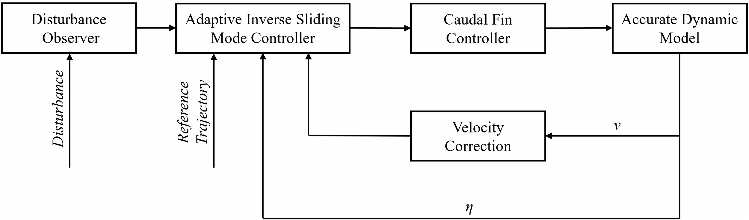
Trajectory tracking control diagram of bionic fish.
In the simulation verification, a trajectory tracking task for sinusoidal curves was designed. The controller parameters , , , , , and the nonlinear disturbance observer gain parameter . The desired trajectory is: , defining the initial velocity of the machine fish m, define the initial position of the robotic fish as m, define the environmental disturbance and uncertainty as , and define the current perturbation as , and the simulation time is set to 30s. The parameters of the proposed robotic fish model are derived from those of existing robotic fish prototypes, with its physical dimensions specified as length (L) × width (W) × height (H) = 1.6 m × 0.7 m × 0.4 m.
To validate the effectiveness of the nonlinear disturbance observer, the basic inverse sliding mode controller and the controller with the nonlinear disturbance observer are compared under the same initial conditions. The simulation results are presented in Figure 4.
Figure 4
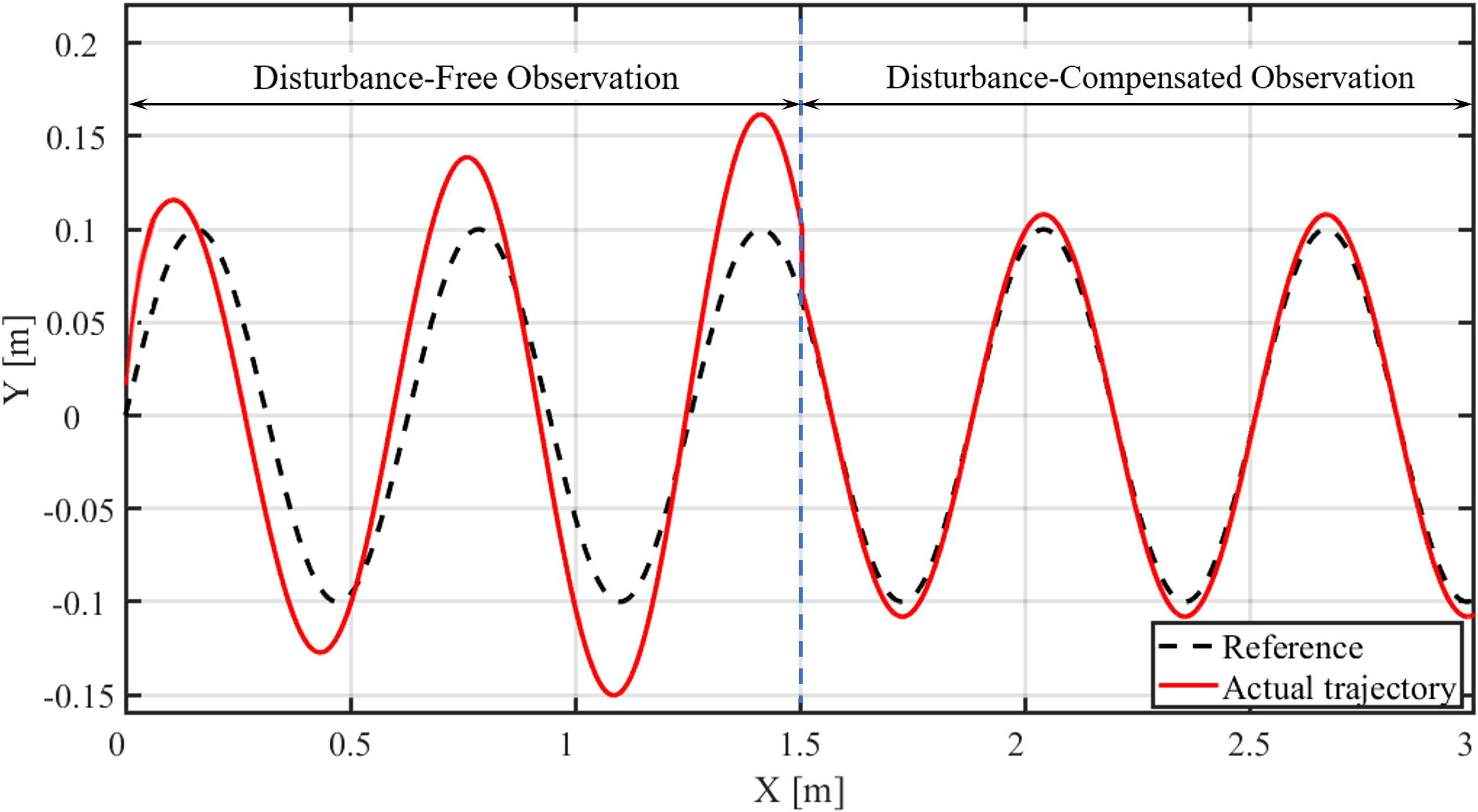
Effect of nonlinear interfering observer.
Figure 4 demonstrates that, in the absence of the nonlinear disturbance observer, the error between the actual and reference trajectories exhibits a monotonic increase within the 0–15 s interval (approximately 1.5 m forward displacement), indicating that model uncertainties and external disturbances significantly affect the dynamic behavior of the robotic fish. Upon the introduction of the nonlinear disturbance observer at 15 s, the system’s transient response quickly converges over a minimal transition distance, with the error amplitude rapidly decaying and remaining at a very low level for the subsequent 15 s. This result validates the nonlinear disturbance observer’s ability to provide accurate online estimation and real-time compensation for aggregate disturbances. Quantitative analysis further shows that, with the controller gain held constant, the incorporation of the nonlinear disturbance observer reduces trajectory tracking error by approximately 95.6%, while effectively mitigating periodic disturbances induced by nearshore wave forces and sediment disturbances. These findings significantly enhance both the trajectory tracking accuracy and robustness of the robotic fish.
To verify the advantages of the disturbance observer - based inverse sliding mode control over the conventional sliding mode control with observer, this paper conducts simulation experiments of the two control methods after introducing near - sea area disturbances, as shown in Figure 5.
Figure 5
![Graph showing three curves representing system responses over time with X-axis labeled “X [m]” and Y-axis labeled “Y [m]”. The intervals are marked as “Disturbance-Free” and “Post-Disturbance Introduction.” The legend identifies curves as reference (black dashed), conventional sliding mode (blue dotted), and disturbance observer-based inverse sliding mode (red solid).](https://www.frontiersin.org/files/Articles/1691667/xml-images/fmars-12-1691667-g005.webp)
Comparison between conventional sliding mode control with observer and disturbance observer - based inverse sliding mode control.
Figure 6 shows that both the conventional sliding mode control with observer and the disturbance observer-based inverse sliding mode control achieve good tracking performance in a disturbance-free environment. However, for the conventional sliding mode control with observer, the error between the actual trajectory and the reference trajectory expands significantly within the Post-Disturbance Introduction Interval. When the disturbance observer-based inverse sliding mode control is activated, the system’s tracking performance stabilizes rapidly over a very short distance. The error amplitude decreases sharply and remains at an extremely low level throughout the entire interval. This result confirms that the disturbance observer-based inverse sliding mode control can accurately counteract the effects of offshore disturbances. Quantitative analysis further indicates that, under otherwise identical conditions, compared with the conventional sliding mode control with observer, the adoption of the disturbance observer-based inverse sliding mode control reduces the trajectory tracking error by approximately 82.3%, effectively improving both the trajectory tracking accuracy and robustness of the robotic fish.
Figure 6
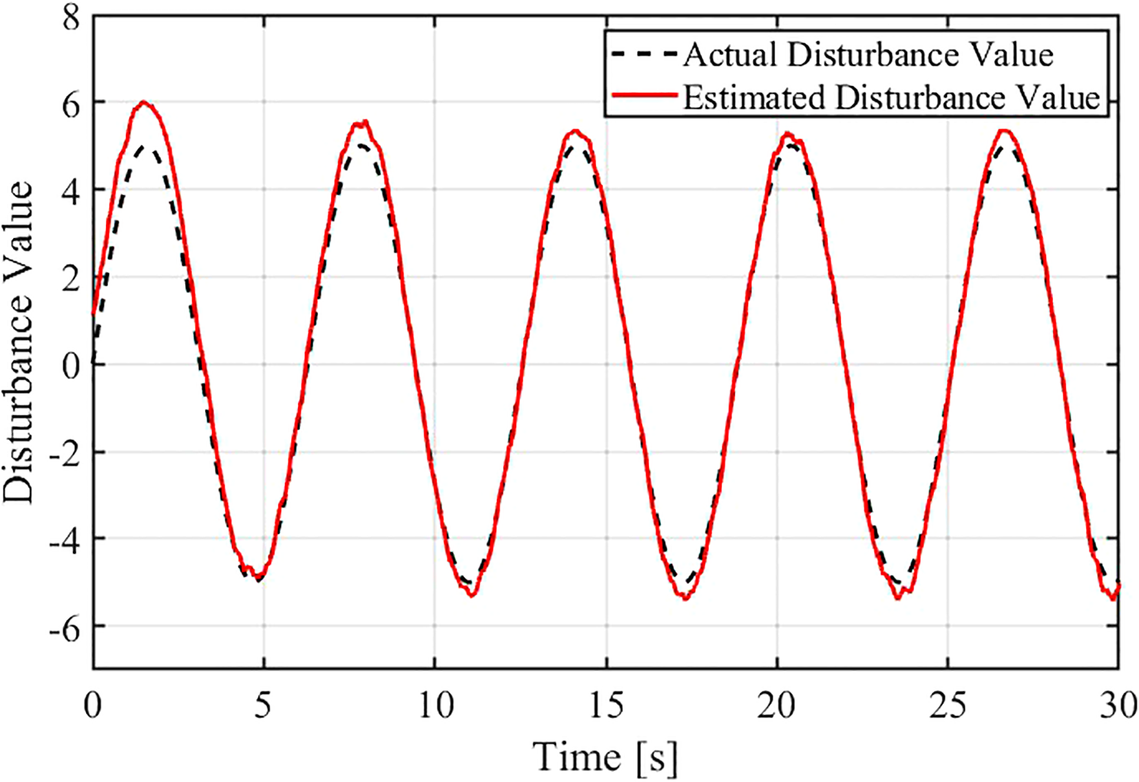
Actual disturbance vs. estimated disturbance.
To evaluate the effectiveness of the designed controller, the output data for the controller with the interference observer is analyzed. Figure 6 shows the comparison between the actual input interference value and the observed estimated interference value from the nonlinear disturbance observer. The results indicate that the observed interference value can accurately track the actual interference and reaches a steady state after approximately 3 seconds. After this transient period, the two values coincide closely. Although there is a transient fluctuation when the interference signal changes suddenly (with a peak error of about 10%), the observer quickly restores stable tracking, demonstrating good dynamic response capability. Only small high-frequency fluctuations are observed in the steady-state phase (amplitude < 2%), and the overall tracking error is less than 5%, verifying the effectiveness of the designed controller. The error is less than 5%, verifying the accuracy and robustness of the interference observer. The simulation results show that the observed interference value closely matches the given interference value. After approximately 3 seconds of pre-estimation time, the interference curve stabilizes and coincides with the actual interference value.
The following demonstrates the effectiveness of the adaptive inverse sliding mode controller, with Figure 7 showing the comparison between the actual current velocity and the observed velocity from the controller. The simulation results show that, under a strong current velocity of 3 m/s, the controller remains in the pre-estimation stage with minimal changes during the first 1 second. At around 1.5 seconds, it begins to rise sharply, approaching the given actual current velocity, and stabilizes after a short adjustment within approximately 3 seconds, aligning closely with the given actual current value.
Figure 7
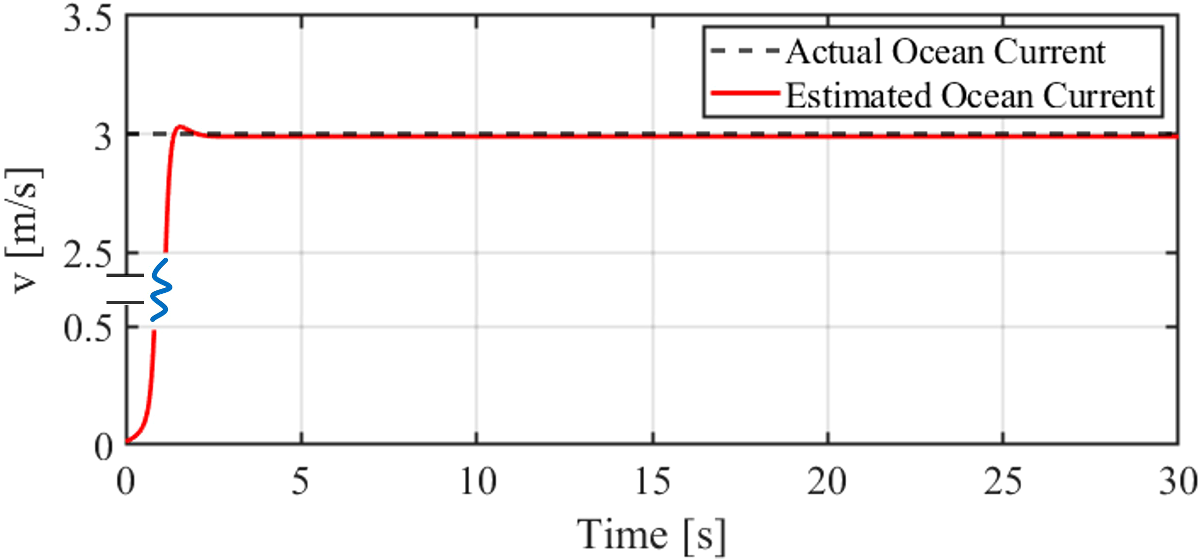
Actual current speed vs. estimated current speed.
As shown in Figure 8, the trajectory tracking error reveals that, in the initial stage of the simulation, there is a large error due to the difference between the initial position and the starting point of the desired trajectory. After 2 seconds, the trajectory tracking error is less than 0.01 m, which is about 2.2% of the robotic fish’s body length. The error exhibits periodic fluctuations with small amplitude due to external perturbations. This demonstrates that the controller can effectively compensate for the steady-state error and has good dynamic disturbance suppression capability.
Figure 8
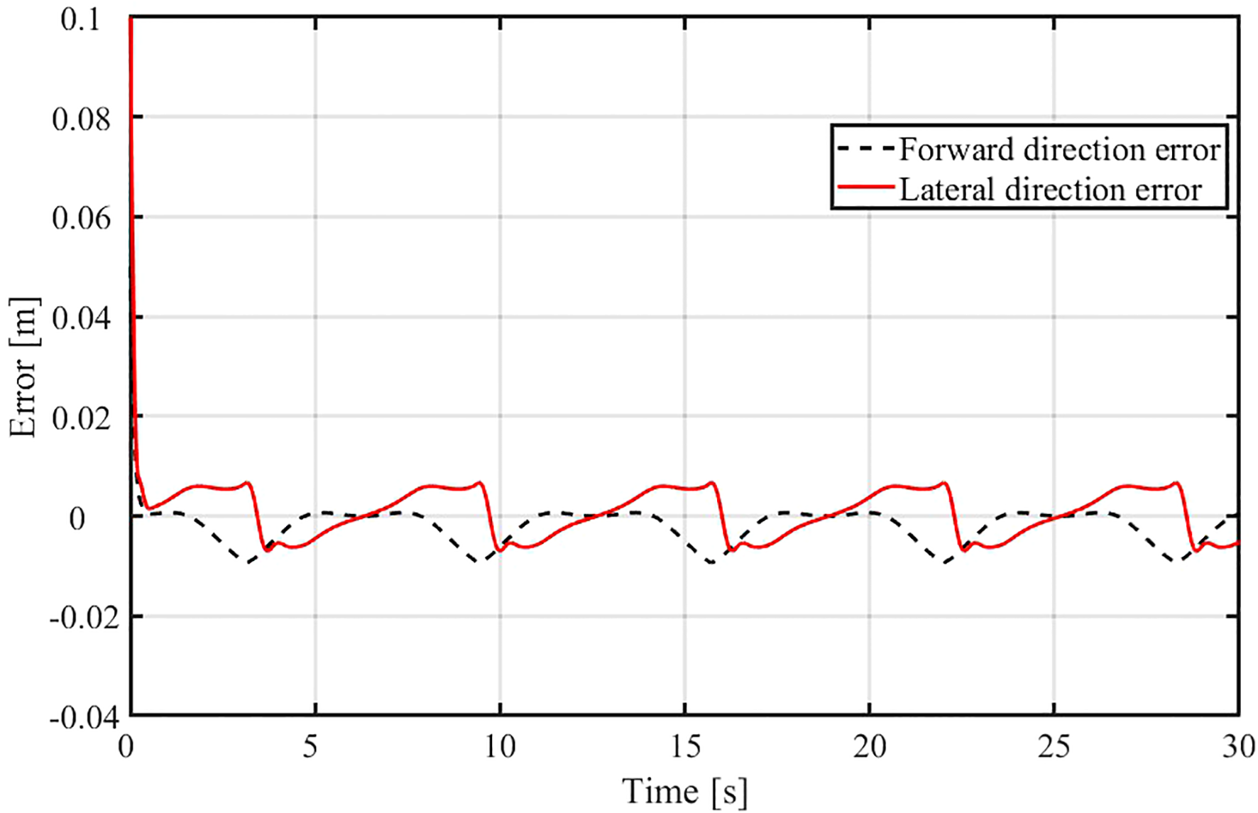
Trajectory tracking error.
To evaluate the effectiveness of the velocity correction controller, the velocity output data of the robotic fish is analyzed. Figure 9 presents the simulation results of the robotic fish velocity under the DOB-ASMC controller. Specifically, Figure 9A illustrates the forward speed variation, while Figure 9) illustrates the lateral speed variation of the robotic fish. As shown in Figure 9A, the forward speed of the robotic fish exhibits periodic fluctuations, ranging approximately from 0.05 m/s to 0.15 m/s. This periodic fluctuation results from the robotic fish mimicking the swinging motion of real fish to achieve effective propulsion. Despite the fluctuations, the forward velocity remains above 0.05 m/s, consistent with the characteristic that the robotic fish can only swim forward. Figure 9B shows that the lateral velocity of the robotic fish fluctuates periodically between -0.03 m/s and 0.02 m/s. This fluctuation reflects the velocity variation during lateral maneuvers, indicating that the robotic fish can flexibly perform side movements in an underwater environment.
Figure 9
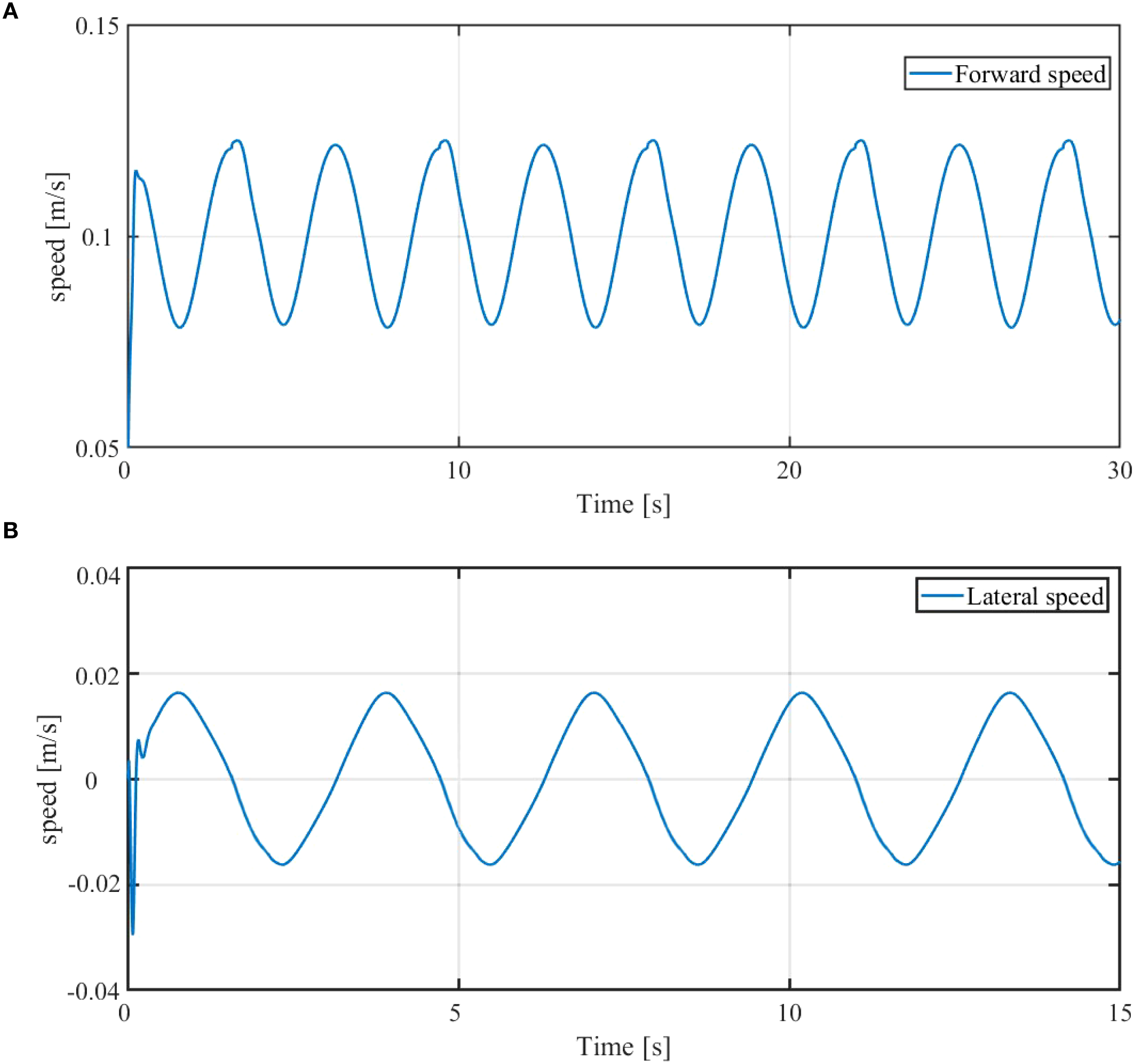
Velocity change of machine fish. (A) Forward speed of the robot fish, (B) Lateral speed of the robot fish.
The tracking error of the robotic fish’s velocity is analyzed below, as shown in Figure 10. Figure 10A illustrates the forward velocity error, while Figure 10B shows the lateral velocity error. The simulation results show that the forward velocity error exhibits small periodic fluctuations between approximately -0.004 m/s and 0.001 m/s. These fluctuations are caused by the swinging motion used by the robotic fish to mimic real fish swimming, and also reflect the dynamic response characteristics of the velocity correction system as it adjusts the robotic fish’s velocity to match the target. In contrast, the lateral velocity error remains close to zero, except during the initial phase, which is attributed to the small magnitude and slow variation of the lateral velocity. Both forward and lateral velocity errors remain within a small range, indicating that the velocity control system exhibits good tracking performance and stability, and can effectively minimize the deviation between the actual and desired velocities of the robotic fish.
Figure 10
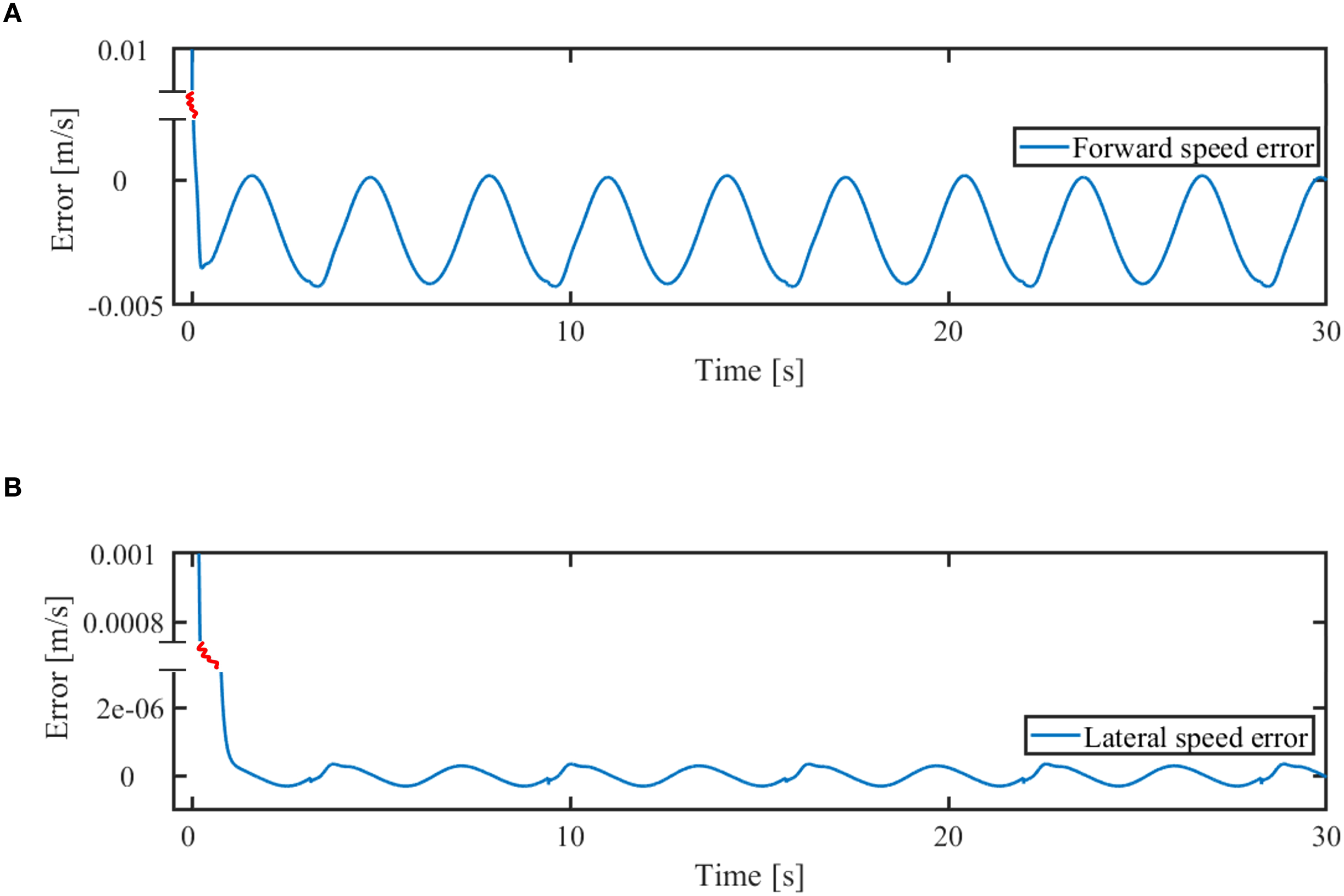
Machine fish speed error. (A) Error in forward speed of robot fish, (B) Error in lateral speed of robot fish
To verify the effectiveness of directly using the tailfin’s swing frequency and bias as control inputs, the tailfin input signals are analyzed, as shown in Figure 11. The caudal fin frequency curve in Figure 11A shows frequent fluctuations between 2.5 Hz and 3.3 Hz, occasionally reaching the saturation upper limit of 3.3 Hz. This saturation mainly occurs when the robotic fish needs to accelerate rapidly or execute highly dynamic maneuvers, such as sharp turns. Notably, the duration of frequency saturation is relatively short, indicating that the controller ensures maneuverability while avoiding potential stability issues associated with prolonged actuator operation in saturated conditions. This control behavior enables the system to respond quickly to sudden commands while maintaining robustness through intermittent saturation. The tailfin bias curve in Figure 11B also exhibits clear saturation behavior, with fluctuations fully covering the design range from –π/4 to π/4 and reaching both limits in several control cycles. Bias saturation primarily occurs in segments with high trajectory curvature, where extreme tailfin deflection is needed to produce sufficient steering torque. Similar to the frequency signal, the bias saturation is impulsive rather than continuous, reflecting the controller’s optimal trade-off between rapid heading adjustment and energy efficiency. Several significant bias fluctuations appear in the bias curve, mainly due to the controller’s input compensation in response to external disturbances. The rapid return to a steady state further demonstrates the controller’s strong robustness.
Figure 11
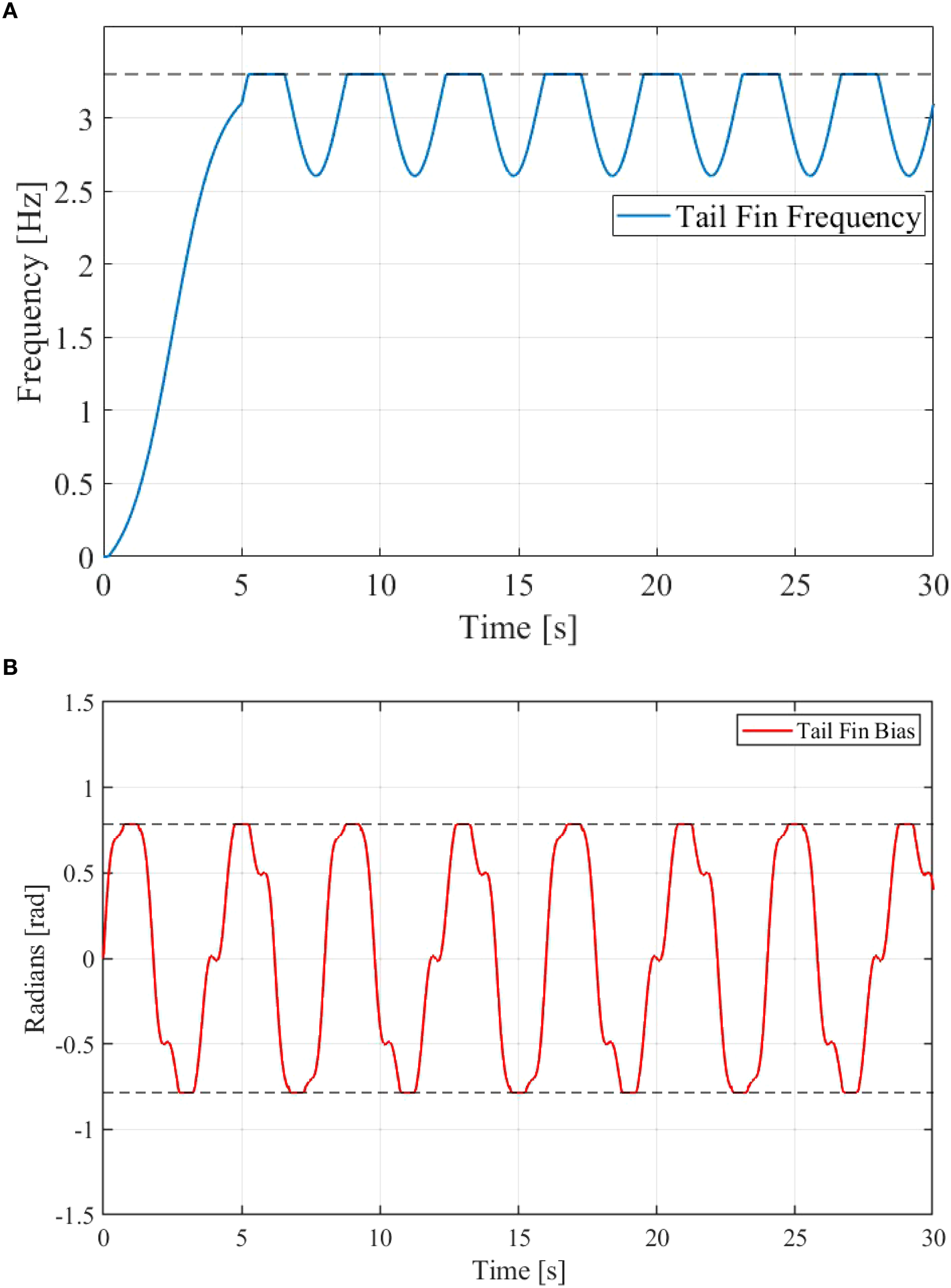
Tail fin input. (A) Frequency, (B) Bias
To evaluate the effectiveness and robustness advantages of the Disturbance Observer-based Adaptive Sliding Mode Control (DOB-ASMC) controller under strong disturbance conditions, this study designs comparative simulation experiments to benchmark its performance against two categories of control methods: one category consists of basic control methods without disturbance compensation, including conventional Proportional-Integral-Derivative (PID) control and standard sliding mode control (SMC); the other category comprises mainstream advanced control methods also integrated with disturbance observers, namely Disturbance Observer-based PID (DOB-PID) control and Disturbance Observer-based Model Predictive Control (DOB-MPC).
For the simulation tests, two types of typical complex trajectory tracking tasks are selected: Archimedean spiral tracking and cloverleaf trajectory tracking. Specifically, Figure 12 focuses on comparing the performance differences between DOB-ASMC and the basic control methods (standard PID, standard SMC); Figure 13 presents the result differences of all comparative methods in the Archimedean spiral trajectory tracking task; and Figure 14 demonstrates the performance comparison of each method in the cloverleaf trajectory tracking task.
Figure 12
Performance comparison between DOB-ASMC and basic control methods.
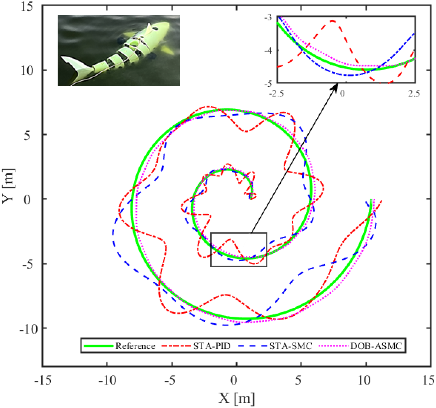
Figure 13
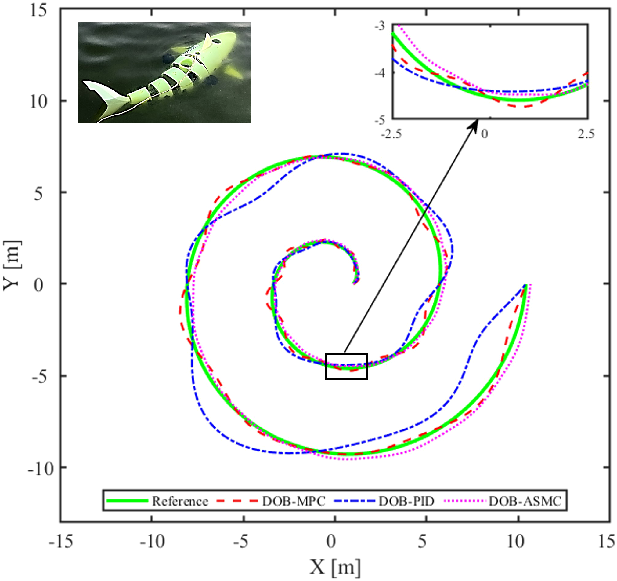
Comparison of spiral trajectory tracking by different control methods.
Figure 14

Comparison of cloverleaf trajectory tracking with different control methods.
where the spiral trajectory is defined by , and the cloverleaf trajectory is defined by . The MPC controller parameters are: , control time domain , prediction time domain , and relaxation factor . The PID controller parameters are: proportional gain , integral gain , differential gain .
Figure 12 depicts the trajectory tracking results of different control methods for a robotic fish under strong disturbance conditions. It can be observed that the STA-PID and STA-SMC trajectories deviate significantly from the reference trajectory, with large fluctuations and obvious tracking errors. In contrast, the DOB-ASMC trajectory is much closer to the reference trajectory. The local magnification in the upper right corner further illustrates that DOB-ASMC maintains a very small deviation from the reference trajectory throughout the tracking process, while the other two methods exhibit larger deviations. This indicates that the DOB-ASMC controller demonstrates superior trajectory tracking accuracy and robustness under strong disturbances compared to STA-PID and STA-SMC.
As shown in Figure 13, the DOB-ASMC controller closely follows the reference trajectory, with the tracking path nearly overlapping it—particularly evident in the zoomed-in view. It is evident that this control method provides higher accuracy and lower fluctuation compared to the other control strategies, indicating its superior accuracy and robustness in tracking complex trajectories. Although the DOB-MPC controller exhibits relatively stable tracking performance, its control output displays noticeable steady-state fluctuations, revealing that its control architecture is inherently less robust against high-intensity external disturbances. In contrast, the DOB-PID controller demonstrates poor tracking performance, particularly in certain segments of the trajectory, with noticeable deviations. This is mainly attributed to the lack of robustness of PID control when subjected to system parameter variations and external disturbances.
As shown in the simulation results in Figure 14, the DOB-ASMC control method exhibits noticeable tracking errors in regions with high reference trajectory curvature. This phenomenon is primarily attributed to two factors: (1) the dynamics of the robotic fish’s tail-fin propulsion system introduce an inherent response delay during high-speed steering; and (2) actuator input saturation constraints further limit the system’s instantaneous steering capability. However, the DOB-ASMC controller still demonstrates excellent tracking accuracy and robustness in trajectory segments with low curvature. In contrast, the other control methods are more susceptible to disturbances and exhibit poorer trajectory tracking performance. Although the DOB-MPC controller exhibits relatively small overall fluctuation amplitudes, it faces two major issues during the recovery phase following a trajectory deviation: (1) the transient process required to return to the desired trajectory is prolonged; and (2) significant oscillations persist during the transition. Specifically, when the system deviates from the reference trajectory, the controller exhibits slow convergence, and high-frequency oscillations cannot be effectively suppressed during this process. Moreover, the DOB-PID controller shows poor performance in terms of both tracking accuracy and robustness.
5 Conclusion
To address the demand for highly robust trajectory tracking control of a bionic robotic fish operating in a strongly perturbed underwater environment near coastal areas, this paper proposes an adaptive inverse sliding mode control method based on a disturbance observer. The controller incorporates the dynamic model of total disturbances and the caudal fin force formulation, and directly uses the caudal fin oscillation frequency and bias as control inputs. The following main conclusions are drawn based on simulation results:
-
The disturbance observer designed in this paper, which relies on a single gain parameter K for convergence accuracy, is simple yet effective. It can accurately compensate for disturbances and model uncertainties, thereby improving the stability of the control system. In addition, the inverse sliding mode controller adaptively compensates for strong near-sea currents, enabling rapid convergence and accurate current estimation that closely matches the actual environmental conditions.
-
In trajectory tracking performance tests, the proposed control system demonstrates strong convergence characteristics and robustness. The tracking error remains significantly smaller than the body length of the robotic fish, fully validating the effectiveness of the proposed control algorithm.
-
The speed correction module in the controller enables effective velocity regulation of the robotic fish. The system maintains a small tracking error in both forward and lateral directions, particularly during the stabilization phase, demonstrating excellent control accuracy and providing a reliable foundation for high-precision trajectory tracking.
-
The tail-fin frequency and bias control strategy effectively enables high-maneuverability motion in the robotic fish. During maneuvering, both frequency and bias signals saturate rapidly to ensure fast dynamic response, while intermittent saturation protects the actuators. The pulsed regulation of bias and the fast recovery from disturbances confirm the controller’s superior balance between agility and robustness.
-
The disturbance observer-based adaptive inverse sliding mode control (DOB-ASMC) significantly outperforms DOB-PID and DOB-MPC in trajectory tracking under strongly perturbed conditions. Its adaptive sliding mode structure effectively suppresses external disturbances and model uncertainties. Furthermore, the integration of a disturbance observer enhances the overall robustness, providing a reliable solution for trajectory tracking of bionic robotic fish in complex underwater environments.
In future work, we plan to determine the optimal controller parameters through optimization analysis and further optimize the control strategy within the saturation range. An adaptive mechanism will be introduced to dynamically adjust saturation limits according to varying operating conditions. Additionally, experimental validation will be conducted to evaluate the trajectory tracking performance of the robotic fish under real-world aquatic conditions using the proposed control method.
Statements
Data availability statement
The original contributions presented in the study are included in the article/supplementary material. Further inquiries can be directed to the corresponding author.
Author contributions
JS: Writing – original draft, Writing – review & editing, Methodology, Conceptualization. YL: Supervision, Methodology, Writing – review & editing, Funding acquisition. FB: Validation, Writing – original draft. XY: Writing – review & editing, Methodology. EQ: Writing – review & editing, Investigation. GX: Supervision, Writing – review & editing, Funding acquisition.
Funding
The author(s) declare that financial support was received for the research, and/or publication of this article. This work is supported by the National Key Research and Development Program of China (2023YFC2810100), the National Natural Science Foundation of China(52471331), the Major Scientific and Technological Project of the Ministry of Water Resources of China (SKS-2022027), the National Natural Science Foundation of China(NSFC)Major Research Program “Monitoring/Sampling/Regulation Technologies and Equipment for Experimental Water Bodies in Marine Carbon Sink Processes” (No42188102).
Conflict of interest
The authors declare that the research was conducted in the absence of any commercial or financial relationships that could be construed as a potential conflict of interest.
Generative AI statement
The author(s) declare that no Generative AI was used in the creation of this manuscript.
Any alternative text (alt text) provided alongside figures in this article has been generated by Frontiers with the support of artificial intelligence and reasonable efforts have been made to ensure accuracy, including review by the authors wherever possible. If you identify any issues, please contact us.
Publisher’s note
All claims expressed in this article are solely those of the authors and do not necessarily represent those of their affiliated organizations, or those of the publisher, the editors and the reviewers. Any product that may be evaluated in this article, or claim that may be made by its manufacturer, is not guaranteed or endorsed by the publisher.
References
1
Behbahani S. B. Tan X. (2017). Design and dynamic modeling of electrorheological fluid-based variable-stiffness fin for robotic fish. Smart Mater. Struct.26, 15. doi: 10.1088/1361-665X/aa7238
2
Cao Y. Li H. Li A. Yin X. Yan X. Zhang L. et al . (2022). Structure design and dynamic analysis of a tensegrity-based carangiform robotic fish. Chin. Sci. Bull.-Chin.67, 4251–4262. doi: 10.1360/TB-2022-0603
3
Clapham R. J. Hu H. (2014). “ Isplash -i: high performance swimming motion of a carangiform robotic fish with full-body coordination,” in 2014 IEEE International Conference On Robotics and Automation (Icra) (IEEE, Hong Kong), 322–327.
4
Kadiyam J. Mohan S. (2019). Conceptual design of a hybrid propulsion underwater robotic vehicle with different propulsion systems for ocean observations. Ocean Eng.182, 112–125. doi: 10.1016/j.oceaneng.2019.04.069
5
Kim D. Lee S. Park J. H. (2008). “ Design of central pattern generators (CPGs) for trajectory tracking of fish-mimetic robots,” in Proceedings of the 7Th Wseas International Conference On Computational Intelligence, Man-Machine Systems and Cybernetics (Cimmacs ‘08) (IEEE, Hong Kong), 191–196.
6
Li D. Sun Y. Zeng L. Law R. Xu Y. Wu E. Q. et al . (2025). Finite-time terminal sliding mode-based formation control scheme for a robotic fish. IEEE Trans. Ind. Inform. doi: 10.1109/TII.2025.3556064
7
Li H. Li L. Wang H. Zhang W. Ren P. (2025). Underwater image captioning with aquaSketch-enhanced cross-scale information fusion. IEEE Trans. Geosci. Remote Sens.63, 1–18. doi: 10.1109/TGRS.2025.3585119
8
Li M. Wei C. Li L. Yuan Z. Liu Y. Xue G. (2025). Numerical study of hybrid systems combining different WECs microarrays based on the TGL semi-submersible floating platform. Front. Mar. Sci.12. doi: 10.3389/fmars.2025.1563310
9
Li S. Wu Z. Dai S. Wang J. Tan M. Yu J. (2024). Tight-space maneuvering of a hybrid-driven robotic fish using backstepping-based adaptive control. IEEE-ASME Trans. Mechatron.29, 3219–3231. doi: 10.1109/TMECH.2023.3338879
10
Lin L. Xie H. Zhang D. Shen L. (2010). Supervised neural Q_learning based motion control for bionic underwater robots. J. Bionic Eng.7, S177–S184. doi: 10.1016/S1672-6529(09)60233-X
11
Ma Y. Li X. Liang B. Du Y. Liu J. Yang S. (2019). “ Development and motion mode analysis of IPMC bionic jellyfish based on app bluetooth remote control,” in 2018 4Th International Conference on Environmental Science and Material Application, vol. 252. (IOP Publishing, Bristol). doi: 10.1088/1755-1315/252/2/022040
12
Mu Y. Qiao J. Liu J. An D. Wei Y. (2022). Path planning with multiple constraints and path following based on model predictive control for robotic fish. Inf. Process. Agric.9, 91–99. doi: 10.1016/j.inpa.2021.12.005
13
Nash J. Z. Bond J. Case M. Mccarthy I. Mowat R. Pierce I. et al . (2021). Tracking the fine scale movements of fish using autonomous maritime robotics: a systematic state of the art review. Ocean Eng.229. doi: 10.1016/j.oceaneng.2021.108650
14
Ning K. Hartono P. Sawada H. (2022). Using inverse learning for controlling bionic robotic fish with SMA actuators. MRS Adv.7, 649–655. doi: 10.1557/s43580-022-00328-w
15
Rehman S. Alhems L. M. Alam M. M. Wang L. Toor Z. (2023). A review of energy extraction from wind and ocean: technologies, merits, efficiencies, and cost. Ocean Eng.267. doi: 10.1016/j.oceaneng.2022.113192
16
Sfakiotakis M. Lane D. M. Davies J. (1999). Review of fish swimming modes for aquatic locomotion. IEEE J. Ocean. Eng.24, 237–252. doi: 10.1109/48.757275
17
Vignesh D. Asokan T. Vijayakumar R. (2024). Performance analysis of a caudal fin in open water and its coupled interaction with a biomimetic AUV. Ocean Eng.291. doi: 10.1016/j.oceaneng.2023.116348
18
Wang H. Zhang W. Ren P. (2024). Self-organized underwater image enhancement. ISPRS J. Photogrammetry Remote Sens.215, 1–14. doi: 10.1016/j.isprsjprs.2024.06.019
19
Wang H. Zhang W. Xu Y. Li H. Ren P. (2026). WaterCycleDiffusion: Visual–textual fusion empowered underwater image enhancement. Inf. Fusion127, 103693. doi: 10.1016/j.inffus.2025.103693
20
Wang J. Chen S. Tan X. (2013). Control-oriented averaging of tail-actuated robotic fish dynamics. 2013 Am. Control Conf. (ACC), 591–596. doi: 10.1109/ACC.2013.6579901
21
Wang K. Chen G. Wang Q. Zhong Y. (2024). Investigation on target point approaching control of bionic robotic fish in static flow. Ocean Eng.304. doi: 10.1016/j.oceaneng.2024.117876
22
Wang M. Wang K. Zhao Q. Zheng X. Gao H. Yu J. (2023). LQR control and optimization for trajectory tracking of biomimetic robotic fish based on unreal engine. Biomimetics8. doi: 10.3390/biomimetics8020236
23
Wang M. Zhang Y. Dong H. Yu J. (2020). Trajectory tracking control of a bionic robotic fish based on iterative learning. Sci. China Inf. Sci.63. doi: 10.1007/s11432-019-2760-5
24
Wang M. Zhang Y. Yu J. (2022). An SNN-CPG hybrid locomotion control for biomimetic robotic fish. J. Intell. Robot. Syst.105. doi: 10.1007/s10846-022-01664-7
25
Wang N. Zhang Y. Peng L. Zhao W. (2025). Hydrodynamic characteristics study of bionic dolphin tail fin based on bidirectional fluid-structure interaction simulation. Biomimetics10. doi: 10.3390/biomimetics10010059
26
Wang Q. Hong Z. Zhong Y. (2022). Learn to swim: online motion control of an underactuated robotic eel based on deep reinforcement learning. Biomimetic Intell. Robotics2. doi: 10.1016/j.birob.2022.100066
27
Wang Q. Zhang J. Huang P. Zhong Y. (2025). Design and modeling of a robotic fish with modular adaptive variable stiffness passive joint. IEEE-ASME Trans. doi: 10.1109/TMECH.2025.3562878
28
Wang R. Wang M. Zhang Y. Zhao Q. Zheng X. Gao H. et al . (2023). Trajectory tracking and obstacle avoidance of robotic fish based on nonlinear model predictive control. Biomimetics8. doi: 10.3390/biomimetics8070529
29
Wang Y. Wang J. Kang S. Yu J. (2024). Target-following control of a biomimetic autonomous system based on predictive reinforcement learning. Biomimetics9. doi: 10.3390/biomimetics9010033
30
Wei D. Hu S. Zhou Y. Ren X. Huo X. Yin J. et al . (2023). A magnetically actuated miniature robotic fish with the flexible tail fin. IEEE Robot. Autom. Lett.8, 6099–6106. doi: 10.1109/LRA.2023.3300283
31
Xie F. Li Z. Ding Y. Zhong Y. Du R. (2020). An experimental study on the fish body flapping patterns by using a biomimetic robot fish. IEEE Robot. Autom. Lett.5, 64–71. doi: 10.1109/LRA.2019.2941827
32
Xie F. Zhong Y. Du R. Li Z. (2019). Central pattern generator (CPG) control of a biomimetic robot fish for multimodal swimming. J. Bionic Eng.16, 222–234. doi: 10.1007/s42235-019-0019-2
33
Yan S. Wu Z. Wang J. Feng Y. Yu L. Yu J. et al . (2024). Recent advances in design, sensing, and autonomy of biomimetic robotic fish: a review. IEEE-ASME Trans. Mechatron. doi: 10.1109/TMECH.2024.3469953
34
Yan X. Ma Y. (2023). A distributed control method for flexible robotic fish based on PDE. IET Contr. Theory Appl.17, 1930–1943. doi: 10.1049/cth2.12485
35
Yan Z. Yang H. Zhang W. Lin F. Gong Q. Zhang Y. (2022). Bionic fish tail design and trajectory tracking control. Ocean Eng.257. doi: 10.1016/j.oceaneng.2022.111659
36
Zhang P. Wu Z. Meng Y. Tan M. Yu J. (2020). Nonlinear model predictive position control for a tail-actuated robotic fish. Nonlinear Dyn.101, 2235–2247. doi: 10.1007/s11071-020-05963-2
Summary
Keywords
inverse sliding mode control, nonlinear disturbance observer, trajectory tracking, tail-fin-driven robotic fish, adaptive robust control
Citation
Sun J, Liu Y, Bai F, Yan X, Quan E and Xue G (2025) Trajectory tracking control of robotic fish in offshore disturbance environments via disturbance observer-based inverse sliding mode. Front. Mar. Sci. 12:1691667. doi: 10.3389/fmars.2025.1691667
Received
24 August 2025
Accepted
29 September 2025
Published
22 October 2025
Volume
12 - 2025
Edited by
Ting Zou, Memorial University of Newfoundland, Canada
Reviewed by
Mingxin Liu, Guangdong Ocean University, China; Hao Wang, Laoshan National Laboratory, China
Updates
Copyright
© 2025 Sun, Liu, Bai, Yan, Quan and Xue.
This is an open-access article distributed under the terms of the Creative Commons Attribution License (CC BY). The use, distribution or reproduction in other forums is permitted, provided the original author(s) and the copyright owner(s) are credited and that the original publication in this journal is cited, in accordance with accepted academic practice. No use, distribution or reproduction is permitted which does not comply with these terms.
*Correspondence: Gang Xue, sduxuegang@163.com
Disclaimer
All claims expressed in this article are solely those of the authors and do not necessarily represent those of their affiliated organizations, or those of the publisher, the editors and the reviewers. Any product that may be evaluated in this article or claim that may be made by its manufacturer is not guaranteed or endorsed by the publisher.