Sediment dynamics in shallow water under wave-current interaction: a case study of Haiyang Beach

As a critical interface in coastal systems, the intertidal zone presents complex sediment dynamics, yet the precise mechanisms governing resuspension and transport under combined wave-current interactions are not fully resolved. Utilize a comprehensive observation system that incorporates both acoustic and optical equipment, we captured concurrent hydrodynamic and sediment data across a full tidal cycle. By applying wave-turbulence decomposition, we successfully isolated the distinct contributions of various forcing mechanisms. Our results unequivocally demonstrate that turbulence is the primary driver of sediment resuspension, superseding the effects of direct wave orbital motion and mean current shear, as confirmed through both regression and wavelet analyses. Moreover, we distinguish between local and net processes: while resuspension is a locally forced phenomenon, net sediment transport is governed by the mean flow. During our observations, the net cross-shore transport was persistently offshore, driven by the combination of ebb tidal currents and wave-induced undertow. Ultimately, these findings challenge the paradigm of wave-dominated sediment processes on tidal flats, underscoring the pivotal role of turbulence in modulating sediment dynamics and offering a more refined perspective on the local sediment budget.

1 Introduction

Intertidal zone, situated at the land-sea interface, are among the most dynamic sedimentary environments on Earth. They not only provide critical ecosystem services but also act as natural buffers protecting coastlines from erosion and storm surges (Barbier et al., 2011; Brand et al., 2020, 2019; Meng et al., 2024; Temmerman et al., 2013). The morphological stability of these systems is fundamentally governed by sediment transport processes, which are driven by the complex interplay of tides, waves, and currents (Green and Coco, 2014; Le Hir et al., 2000; Meng et al., 2024). Understanding the mechanisms of sediment resuspension and transport in these zones is therefore paramount for predicting coastal evolution, managing coastal resources, and designing effective coastal protection strategies (Green and Coco, 2014; Xie et al., 2021).

Sediment dynamics in intertidal environments are notoriously complex due to the superposition of oscillatory wave orbital motions and quasi-steady currents (e.g., tidal currents, wind-driven currents). The combined wave-current flow enhances bottom shear stress, significantly increasing the potential for sediment resuspension compared to conditions of either waves or currents acting alone (Fugate and Friedrichs, 2002; Grant and Madsen, 1979; Li et al., 2022; Liu et al., 2020; Sun et al., 2022; Zhu et al., 2016). While this synergistic effect is well-established, the precise contribution of each component—mean currents, wave orbital velocities, and wave-induced turbulence—to the total shear stress and subsequent sediment response remains a subject of active research and debate (Bian et al., 2018; Fan et al., 2019; Li et al., 2022; Niu et al., 2023b). Early models often parameterized the combined stress using simple additive approaches, but recent studies have highlighted the importance of nonlinear interactions, particularly the generation of turbulence within the wave-current bottom boundary layer (Fan et al., 2019; Niu et al., 2023a; Yuan et al., 2009).

A significant knowledge gap persists in quantifying the role of turbulence as a mediating factor. While direct wave orbital motion can stir sediment, it is the small-scale, high-frequency turbulent eddies that are often more effective at lifting and maintaining sediment in suspension (Sun et al., 2022). However, decomposing the flow field to isolate the turbulent component from the organized wave motion in field settings is challenging. Many previous studies on intertidal flats have either focused on tide-dominated or wave-dominated extremes (Barbier et al., 2011; Meng et al., 2024; Xie et al., 2021; Yu et al., 2024), or have used bulk hydrodynamic parameters (e.g., significant wave height) that do not resolve the fine-scale processes responsible for resuspension (Liu et al., 2020). Consequently, the relative importance of wave-induced orbital shear versus turbulence in driving sediment resuspension events in mixed-energy intertidal settings is not well constrained. For instance, some studies suggest wave orbital velocities are the primary driver (Niu et al., 2023b), while others, often from deeper subtidal zones, point to turbulence as the key agent (Meng et al., 2024; Sun et al., 2022; Yuan et al., 2009). This discrepancy highlights the need for high-resolution, in-situ observations that can parse these competing effects within the unique, shallow, and intermittently exposed environment of an intertidal flat.

The Haiyang intertidal flat, characterized by fine-grained sediments and exposure to both significant tidal ranges and moderate wave energy, provides an ideal natural laboratory to address these questions. Unlike many previously studied systems that are either strongly macrotidal or storm-wave dominated, Haiyang represents a mixed-energy environment where the balance between waves, tides, and turbulence is likely to be nuanced. This study leverages high-frequency, co-located measurements of flow velocities and suspended sediment concentrations to investigate sediment dynamics on this representative flat.

The primary objectives of this research are therefore to: (1) To understand the relative contributions of mean current, waves and turbulence to the fluid dynamic energy near the bed during the tidal cycle. (2) Determine the dominant physical mechanism—direct wave action or turbulence—responsible for initiating and sustaining sediment resuspension events. (3) Characterize the net sediment transport and identify the primary drivers (e.g., tidal asymmetry, wave-induced currents) of the residual sediment flux.

By employing advanced time-frequency analysis methods, such as wave turbulence decomposition and wavelet analysis, we aim to provide direct, quantitative evidence to elucidate the mechanisms of sediment resuspension and transport under combined wave-current forcing. The results are expected to refine our understanding of sediment dynamics on mixed-energy tidal flats and improve the parameterization of sediment transport in coastal morphodynamic models.

2 Materials and methods

2.1 Study area

Haiyang Beach is located on the southeastern coast of Shandong Peninsula, adjacent to the Yellow Sea, with the coastline oriented WSW-ENE (Figure 1A). It is a typical barrier-lagoon beach, primarily composed of well-sorted medium-to-fine sands. Lianli Island, located on the eastern side of the beach, is the largest artificial island in north China and is connected to the mainland via the bridge.

Figure 1

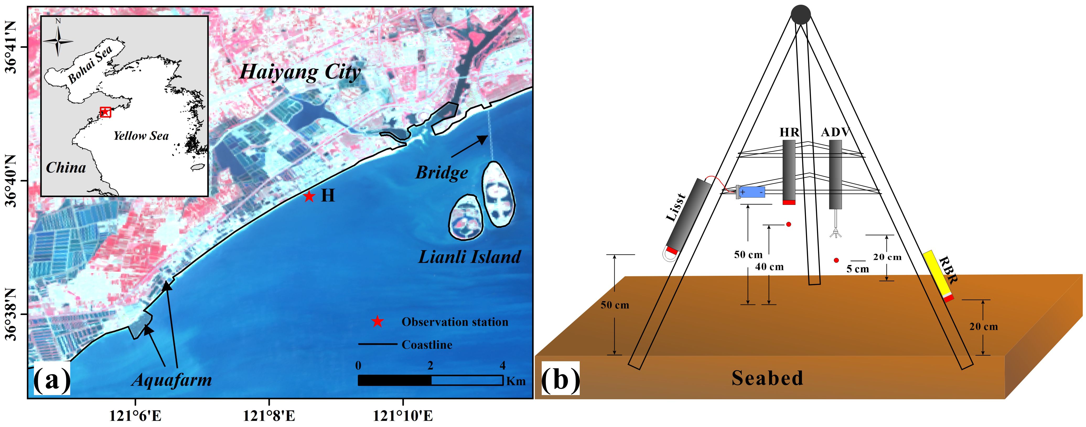
Figure 1. (a) Location of the study area (station H is the bottom-mounted observation station); (b) Schematic diagram of station H and the observation instrumentation.

Haiyang City experiences a warm-temperate East Asian monsoon climate, characterized by southerly winds in spring/summer and northerly winds in autumn/winter. The annual average wind speed is 3.2 m/s, and it is affected by typhoons an average of 1.1 times per year (Yu et al., 2022). It belongs to the regular semi-diurnal tidal, dominated by rectilinear currents with a predominant E-W orientation. The mean low and high tidal levels are -1.20 m and 1.21 m, respectively (Zhang et al., 2021). The waves are mainly wind-driven, and 90% of wave heights are less than 1 m. The normal wave direction is SSW, the strong wave direction is SE, and the maximum wave height is 5.8 m. The annual alongshore sediment transport rate in the study area ranges from 0.16 to 0.19 × 10⁶ m³, primarily directed ENE (Ren et al., 2016).

2.2 Field observations

To obtain sediment dynamics and hydrodynamics in shallow water, a bottom-mounted observation station H was deployed in the intertidal zone of Haiyang Beach from June 27 to 29, 2022 (during the spring tide), which was located at 121.1434°E, 36.6628°N, as shown in Figure 1A. The station was designed as a triangular frame (Figure 1B) and equipped with several instruments.

The Acoustic Doppler Velocimetry (ADV, Nortek 6 MHz) was used to measure near-bed flow velocity components, critical for estimating shear stress and turbulence related to sediment resuspension under wave-current interaction. Currently, ADV is widely applied in the measurement of bottom layer velocity in estuarine and coastal areas (Fugate and Friedrichs, 2002; Kim et al., 2000; Li et al., 2022; Meng et al., 2024; Sun et al., 2022; Xiong et al., 2020; Yang et al., 2016; Zhu et al., 2016). The ADV sensor was positioned 0.2 m above the seabed. The sampling mode was set to burst mode with a sampling frequency of 32 Hz. Each sampling session lasted 600 s, with a sampling interval of 1800 s.

The wave gauge (RBR solo³ D | wave 16) was used to obtain high-frequency pressure for calculating wave parameters and water levels. The sensor was positioned 0.2 m above the seabed, operating in burst mode with a sampling frequency of 16 Hz. Each sampling session lasted 1024 s, with a sampling interval of 1800 s.

The Laser In Situ Scattering and Transmissometry (LISST-200X) was used to acquire high-resolution suspended particle volume concentration data. The sensor was positioned 0.5 m above the seabed, with a sampling frequency of 1 Hz for continuous sampling. The particle size range measured by LISST was from 1 μm to 500 μm, with 36 logarithmically distributed size classes. Due to battery capacity limitations, LISST data were available from 21:00 on June 27 to 18:00 on June 28, while other instruments covered the entire observation period.

All instruments were synchronized to initiate measurements at 21:00 on June 27 and secured at the waterline during the lowest tidal phase to ensure temporal consistency. Additionally, wind field data were obtained from the National Center for Environmental Prediction Climate Forecast System Version 2 (NCEP-CFSv2) provided by the United States National Environmental Prediction Center (URL: https://rda.ucar.edu/datasets/ds094.1/index.html#!access). The spatial resolution of the dataset is 0.2°, and the temporal resolution is 1 hour.

2.3 Analysis methods

2.3.1 Wave-turbulence decomposition

The three dimensions velocity data (u,v,w) recorded by the ADV needs to mitigate the influence of ambient hydrodynamic noise. Spikes in raw data were detected and replaced using the three-dimensional phase-space method (Goring Derek and Nikora Vladimir, 2002). These spikes typically exhibited low correlation coefficients and signal-to-noise ratios ($SNR$), consistent with results from conventional threshold-based denoising methods (e.g., correlation coefficient and $SNR$ filtering). For each burst, data segments with spike replacements exceeding 50% of the total length were discarded. The above workflow was systematically applied to all velocity components (u, v, and w) to ensure data reliability.

Take u as an example, the processed velocity data can be decomposed into mean velocity ($\overline{u}$) and fluctuating velocity ($u^{\prime }$) (Fan et al., 2019). When wave influences are present, the fluctuating velocity $u^{\prime }$ can be further decomposed into wave-induced velocity $u_w^{\text{'}}$ and turbulence-induced velocity $u_t^{\text{'}}$ (Equation 1):

$\begin{array}{ll}u=\overline{u}+u^{\prime }=\overline{u}+u_w^{\text{'}}+u_t^{\text{'}}& (1)\end{array}$

where $\overline{u}$ represents the burst-averaged (10-minute averaged) velocity. For each burst, the horizontal velocity $U_m$ is used to describe the tidal current speed, and is defined as Equation 2:

$\begin{array}{ll}{U}_m=\sqrt{{(\overline{u})}^2+{(\overline{v})}^2}& (2)\end{array}$

In this study, the corresponding current direction indicates the average direction of the tidal current, and is the angle between $\overline{u}$ and $\overline{v}$.

To accurately isolate velocity components induced by waves and turbulence, wave-turbulence decomposition of fluctuating velocities was implemented. Bian et al. (2018) demonstrated the superiority of the Synchrosqueezed Wavelet Transform (SWT) method. This method operates in the frequency domain. For each 10-minute burst, an energy spectral analysis was performed on the velocity time series. The resulting spectrum typically shows a distinct energy peak in the wave frequency band (e.g., 0.05–2 Hz) and a separate region at higher frequencies following a classic inertial subrange slope, which is characteristic of turbulence. For this study, a cutoff frequency was determined by visual inspection of the velocity spectra, where it consistently fell in the frequency band between the wave energy peak and the onset of the turbulent inertial subrange. Frequencies below this were attributed to waves ($u_w^{\text{'}}$), and frequencies above this were attributed to turbulence ($u_t^{\text{'}}$).

Figure 2 illustrates the wave-turbulence decomposition of the fluctuating velocity during the peak significant wave height (approximately 1.33 m) during the observation period. The results indicate a distinct dominant frequency band within the range of 0.08 to 0.2 Hz (Figures 2A, C), corresponding to typical wave periods of 5-12.5 s. The power spectra of the decomposed components confirmed the effective removal of wave signals from the original fluctuating velocities. However, the turbulence spectrum exhibited a pronounced “energy trough” within the wave-dominated frequency range (Figure 2C). Given the narrow bandwidth of wave influence, turbulence energy loss in this range was negligible (Bian et al., 2018; Sun et al., 2022). This methodology enabled decomposition of fluctuating velocities in all three dimensions (u, v, and w) throughout the measurement period. Furthermore, the turbulence spectrum displayed a clear inertial subrange consistent with Kolmogorov’s “−5/3” scaling law (Kolmogorov, 1968), validating the fidelity of turbulence characterization.

Figure 2

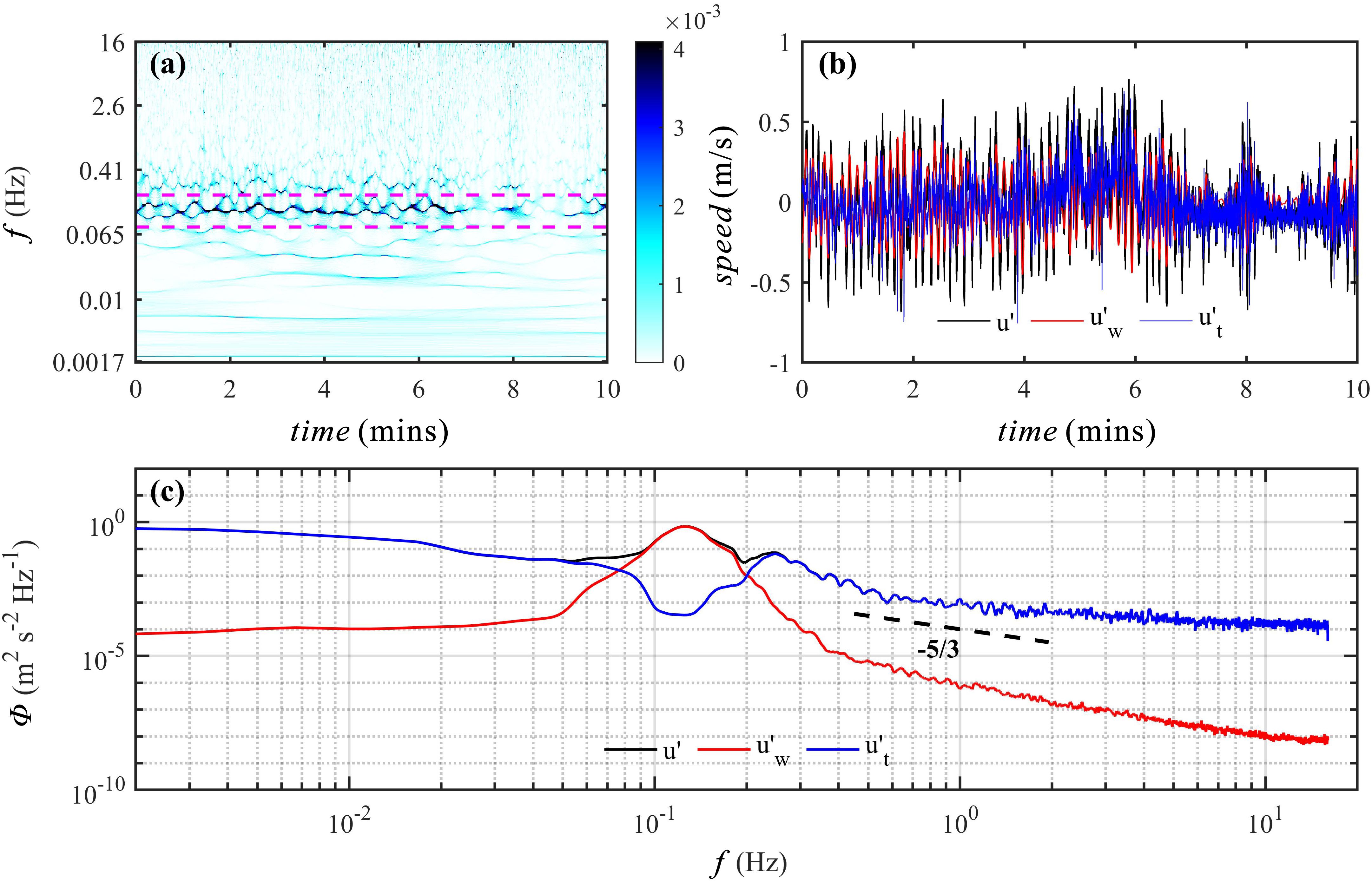
Figure 2. Wave-turbulence decomposition results of fluctuating velocity at Station H (6th burst, significant wave height approximately 1.33 m). (a) SWT analysis of fluctuating velocity, with the purple dashed lines demarcating the wave-dominated frequency range (0.08-0.2 Hz); (b) Time series of $u^{\prime }$ (black line), $u_w^{\text{'}}$ (red line), and $u_t^{\text{'}}$ (blue line); (c) Power spectra of $u^{\prime }$ (black line), $u_w^{\text{'}}$ (red line), and $u_t^{\text{'}}$ (blue line), with the black dashed line representing Kolmogorov’s “−5/3” theoretical spectrum.

2.3.2 Bottom shear stress calculation

The bed shear stress is a critical parameter for studying sediment initiation and transport (Grant and Madsen, 1979; Liu et al., 2020; Yang et al., 2016). The total bottom shear stress ($TSS$) is a combination of stresses induced by wave and turbulence (Bian et al., 2018). Using the decomposed velocity components via SWT, the Reynolds shear stresses were calculated. The turbulence Reynolds stress ($TRS$), wave stress ($WS$) and $TSS$ are given by Equations 3–5:

$\begin{array}{ll}TRS=\rho \sqrt{{(-\overline{u_t^{\text{'}}{w}_t^{\text{'}}})}^2+{(-\overline{v_t^{\text{'}}{w}_t^{\text{'}}})}^2}& (3)\end{array}$

$\begin{array}{ll}WS=\rho \sqrt{{(-\overline{u_w^{\text{'}}{w}_w^{\text{'}}})}^2+{(-\overline{v_w^{\text{'}}{w}_w^{\text{'}}})}^2}& (4)\end{array}$

$\begin{array}{ll}TSS=\rho \sqrt{{(-\overline{u^{\prime }{w}^{\prime }})}^2+{(-\overline{v^{\prime }{w}^{\prime }})}^2}& (5)\end{array}$

where $\rho$ represent the water density, the overline indicates the burst-averaged value.

2.3.3 Acoustic backscatter inversion of suspended sediment volume concentration

The Acoustic Doppler Velocimetry emit fixed-frequency sound waves, and suspended particles in the water column reflect these waves, enabling flow velocity calculation via the Doppler effect. This principle also allows the inversion of suspended sediment concentration (SSC) from acoustic backscatter intensity. Recent advancements in high-frequency ADV measurements have improved understanding of near-bed suspended sediment dynamics (Fan et al., 2019; Niu et al., 2023b; Yuan et al., 2009).

It is generally believed that there is a linear relationship between the $\text{SNR}$ recorded by the ADV and the logarithmic value of SSC (Li et al., 2022; Sun et al., 2022). However, due to challenges in field sediment sampling, this study utilized suspended sediment volume concentration ($TVC$) measured by the LISST as a proxy for SSC. The relationship is expressed as Equation 6:

$\begin{array}{ll}lg(TVC)=a\times SNR+b& (6)\end{array}$

where a and b denote the slope and intercept derived from linear regression.

The relationship between $\text{TVC}$ and the corresponding $\text{SNR}$ is shown in Figure 3A, with a determination coefficient ($R^2$) of 0.8. This allowed the conversion of $\text{SNR}$ into high-frequency suspended sediment volume concentration ($TV{C}_{ADV}$) synchronized with the current. Similar to velocity decomposition (Section 2.3.1), the fluctuating component ($c^{\prime }$) of $TV{C}_{ADV}$ was decomposed into wave ($c_w^{\text{'}}$) and turbulence ($c_t^{\text{'}}$) components using SWT. The power spectra of these components (Figure 3B) exhibited characteristics consistent with those of velocity fluctuations (Figure 2C).

Figure 3

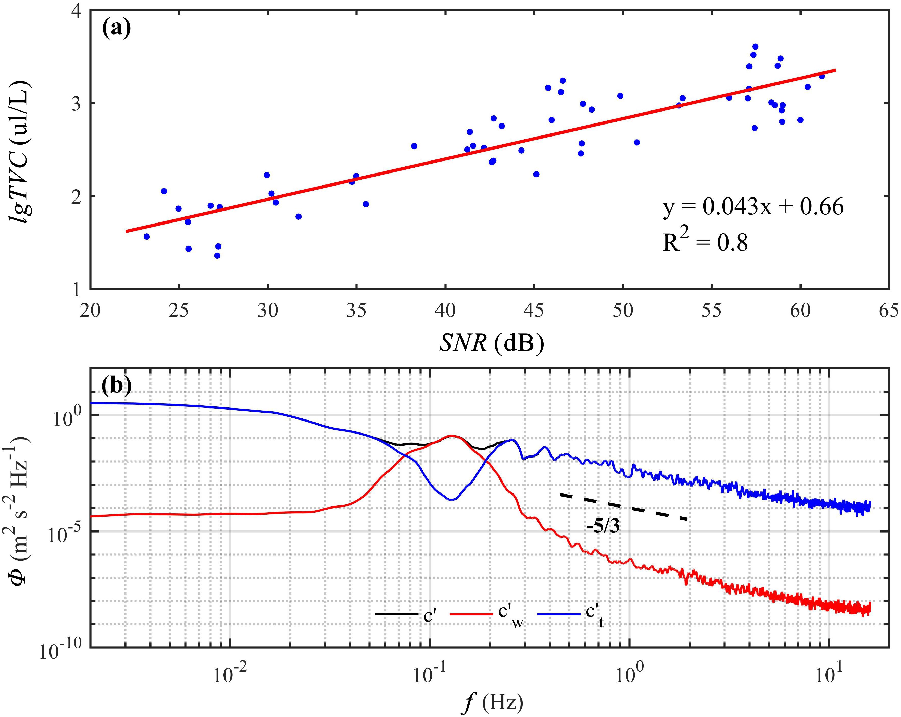
Figure 3. (a) Linear regression relationship between $\text{SNR}$ and $\text{TVC}$; (b) Power spectrum of the $c^{\text{'}}$ (black line), ${\text{c}}_{\text{w}}^{"}$ (red line), and ${\text{c}}_{\text{t}}^{"}$ (blue line) of ${\text{TVC}}_{\text{ADV}}$, with the black dashed line representing Kolmogorov’s “−5/3” theoretical spectrum.

2.3.4 Vertical net flux of suspended sediment

Quantifying the vertical net flux of suspended sediment enables microscale identification of the dominant factors controlling sediment resuspension in the study area. The vertical diffusion flux ($DF=\overline{c^{\prime }{w}^{\prime }}$) consists of two components: the turbulent diffusion flux ($TDF$) and wave-induced diffusion flux ($WDF$), calculated as Equations 7, 8:

$\begin{array}{ll}TDF=\overline{c_t^{\text{'}}{w}_t^{\text{'}}}& (7)\end{array}$

$\begin{array}{ll}WDF=\overline{c_w^{\text{'}}{w}_w^{\text{'}}}& (8)\end{array}$

where $c_t^{\text{'}}$, $w_t^{\text{'}}$, and $c_w^{\text{'}}$, $w_w^{\text{'}}$ denote turbulent and wave-induced components of $TV{C}_{ADV}$ and w, respectively. The overline indicates burst-averaged values.

3 Results and discussion

3.1 Hydrodynamic characteristics

During the observation period, the water level ranged from -1.5 to 1.5 m (0 m is defined as the average water level during the observation period), exhibiting a semi-diurnal tidal pattern with a maximum tidal range of approximately 3 m (Figure 4A). Wind speed gradually decreased from 8 to 2 m/s, while wind direction remained predominantly southerly, except for a brief northerly shift lasting about 4 hours on the morning of June 29 (Figure 4B). The near-bed horizontal current speed ($U_m$) exhibited a negative correlation with water depth, peaking at nearly 0.4 m/s during minimum water depth and approaching zero at maximum depth (Figure 4C). The direction of the current was concentrated between 90° and 180° (east to south). During the observation period, the significant wave height ($H_s$) ranged between 0.3 and 1.4 m, showing a positive correlation with water level. Under the combined influence of peak wind speed and water level, $H_s$ reached its maximum observed value at 04:00 on June 28. Subsequently, as wind speeds generally decreased, the peak $H_s$ associated with high water level also gradually declined. These observations indicate that $H_s$ was primarily wind-controlled, with stronger winds increasing the baseline $H_s$, while tidal variations modulated its magnitude within the tidal cycle. The peak period ($T_p$) remained relatively stable, averaging approximately 8 s. This aligns with the high-energy frequency band (0.08 to 0.2 Hz) observed in the power spectra of velocities and pressure fluctuations (Figure 2C). Notably, the spectral energy peaked at around 0.13 Hz (corresponding to approximately 8 s), confirming waves’ contribution to velocity and pressure fluctuations.

Figure 4

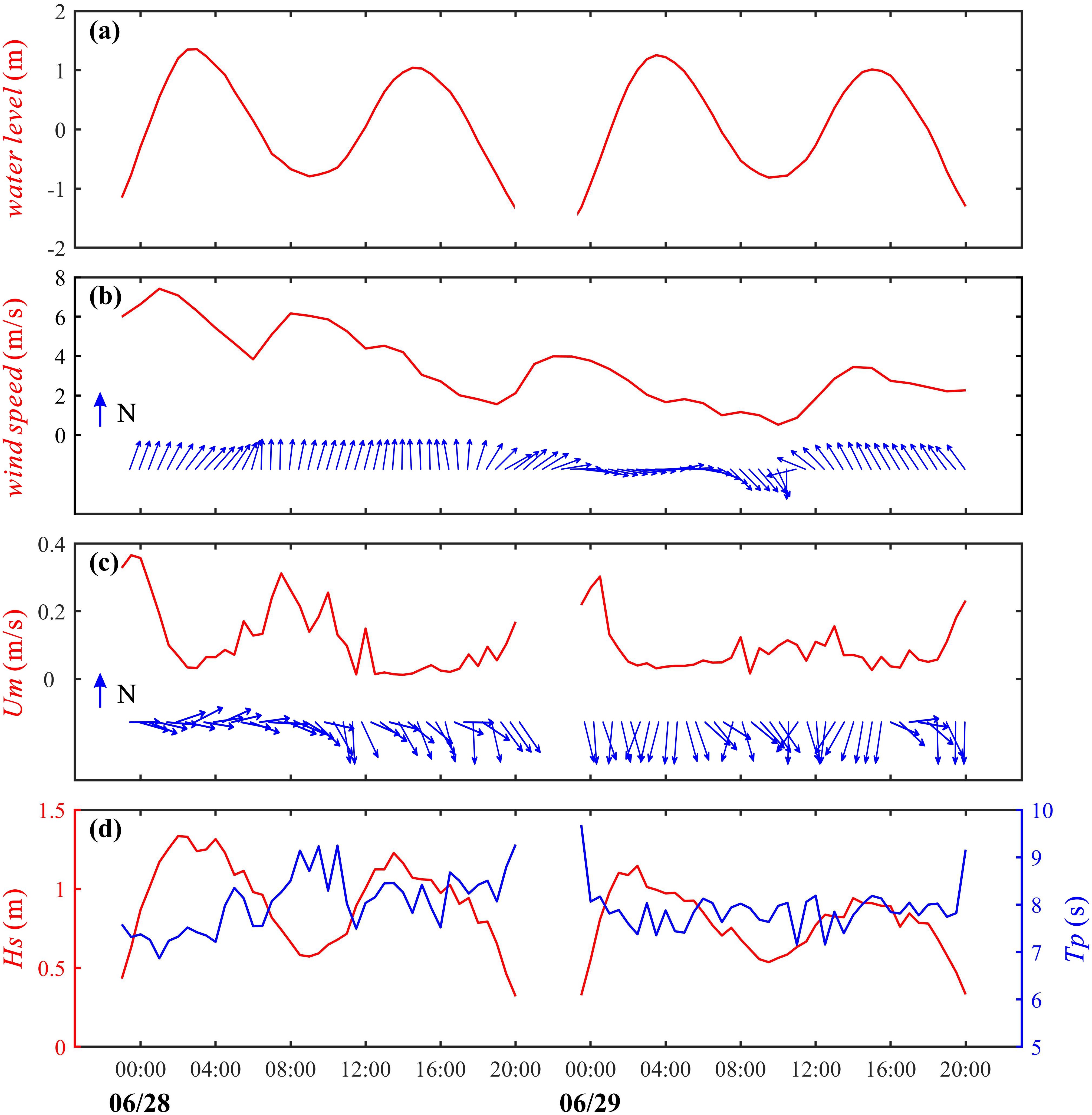
Figure 4. Time series of hydro-meteorological parameters at Station H: (a) Water level; (b) Wind speed and direction; (c) ADV-measured horizontal current speed ($U_m$) and direction; (d) Significant wave height ($H_s$) and spectral peak period ($T_p$). The blue arrows indicate direction only.

3.2 Drivers of sediment resuspension

To identify the controlling factors of sediment resuspension in the intertidal zone, time series data from 00:00 to 18:00 on June 28th (the valid coverage scope for all data) were analyzed (Figure 5). The results show that the significant wave height ($H_s$) and horizontal current speed ($U_m$) are negatively correlated (Figure 5A). $H_s$ peaked during high water levels when $U_m$ was minimal, while $U_m$ increased sharply during ebb tide as water depth decreased and $H_s$ declined. Correspondingly, the total shear stress ($TSS$) closely followed the variability of $U_m$ (Figure 5B), indicating that currents dominated the magnitude of $TSS$. Suspended sediment volume concentration ($TV{C}_{ADV}$) responded synchronously to $TSS$ fluctuations, further confirming current-driven control over sediment dynamics. As shown in the scatter plots, in contrast to the disordered relationship between $TV{C}_{ADV}$ and $H_s$, $TV{C}_{ADV}$ exhibited a positive correlation with $U_m$, although $TV{C}_{ADV}$ ceased to increase when it exceeded 0.2 m/s (Figures 6A, B).

Figure 5

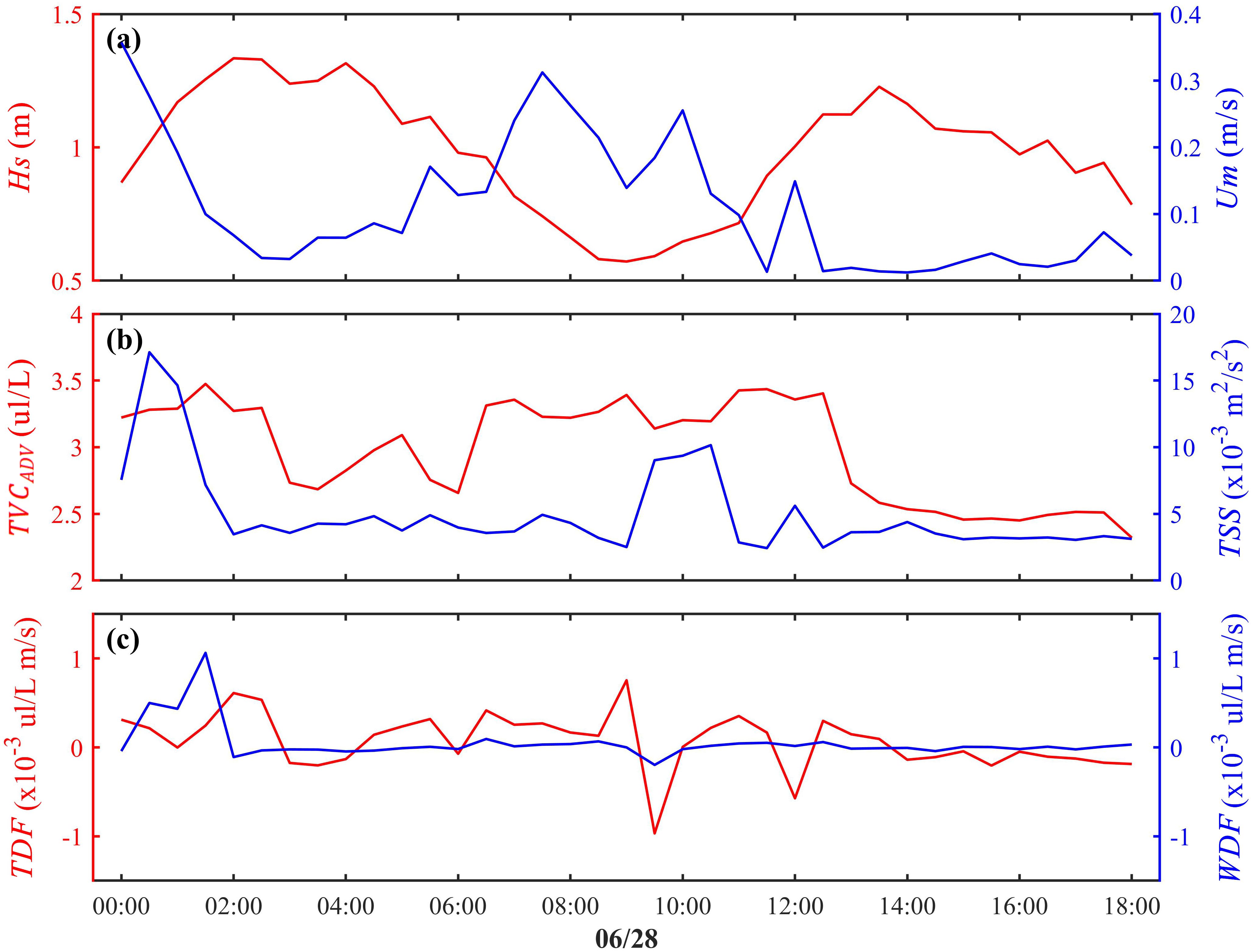
Figure 5. Time series of key parameters from 00:00 to 18:00 on June 28th at Station H: (a) Significant wave height ($H_s$, red line) and horizontal current speed ($U_m$, blue line); (b) Suspended sediment volume concentration ($TV{C}_{ADV}$, red line) and total shear stress ($TSS$, blue line); (c) Vertical turbulent-induced diffusion flux ($TDF$, red line) and wave-induced diffusion flux ($WDF$, blue line).

Figure 6

Figure 6. Scatter plots showing the relationship between the $TV{C}_{ADV}$and various hydrodynamic factors. In each subplot, data points are filtered based on a specific threshold. Data points satisfying the threshold condition are shown in red and were used for the linear regression analysis (light red line), while data points that do not meet the threshold are shown in blue and were excluded from the analysis. The corresponding coefficient of determination ($R²$) for each fit is displayed in red. The subplots correspond to: (a) significant wave height ($H_s$), (b) horizontal velocity ($U_m$), (c) tidal diffusion flux ($TDF$), (d) wave-induced diffusion flux ($WDF$), and (e) total shear stress ($TSS$).

To further explain the resuspension process at the microscale, the vertical turbulent-induced diffusion flux ($TDF$) and vertical wave-induced diffusion flux ($WDF$) were calculated (Figure 5C). The $TDF$ exhibited significantly higher variability than $WDF$, which showed negligible contributions except during 00:00–02:00. This, combined with correlation analysis, suggests that turbulence is the primary driver of vertical sediment exchange. Excluding significant outliers, the correlation between $TDF$ and $TV{C}_{ADV}$ exceeded 0.60, which is markedly higher than the correlations with $WDF$ and $TSS$.

As a further illustration, the high correlation between $TDF$ (as the turbulence-induced vertical sediment diffusion flux) and $TV{C}_{ADV}$ is to be expected. That is, to demonstrate that turbulence dominates resuspension events, it is necessary to establish the correspondence between the instantaneous momentum flux ($TSS$) and the instantaneous sediment diffusion flux ($DF$) in both the time and frequency domains. Wavelet analysis, which can determine the energy distribution of a signal across time and frequency, is widely used for the decomposition and visualization of oceanographic signals and thus provides an ideal tool for this purpose (Li et al., 2022; Sun et al., 2022; Zhang et al., 2022).

Taking a burst event during the highest $TV{C}_{ADV}$ period as an example (June 28th, 10:00), Figure 7 displays the wavelet power spectra (using the Morlet mother wavelet) for $TSS$ and $DF$ (Figures 7A, B), where the analysis passed the 95% confidence test (indicated by the black dashed line). High energy for both $DF$ and $TSS$ was concentrated in the wave-frequency band, dissipating towards higher frequencies. Notably, concurrent and regularly distributed high-energy plume-like structures were observed for $DF$ and $TSS$. These structures were temporally consistent and corresponded to the moment of the strongest $TV{C}_{ADV}$(Figure 7D), highlighting the controlling role of turbulence in sediment resuspension (Li et al., 2022). This is further substantiated by the wavelet coherence analysis of $DF$ and $TSS$, which showed a strong correlation between the two during this period (Figure 7C).

Figure 7

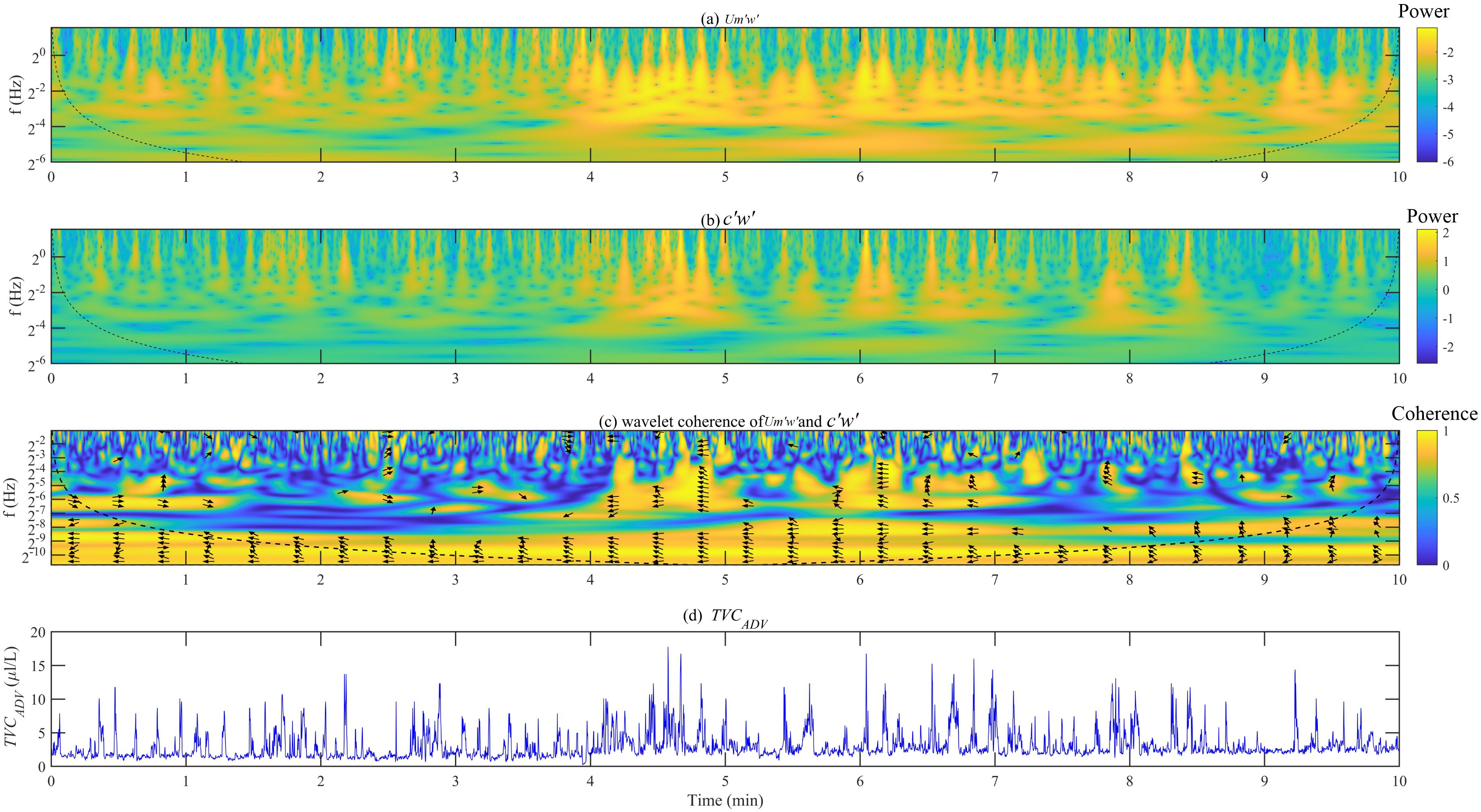
Figure 7. Wavelet power spectra (using the Morlet wavelet) of (a) $TSS$ and (b) $DF$; (c) the wavelet coherence between $TSS$ and $DF$; (d) Time series of $TV{C}_{ADV}$. Note: Black dotted line in (a–c) indicates the cone-of influence caused by edge effects; in (c), when the correlation between the two is greater than 0.75, the phase relationship between them is indicated by arrows. An arrow pointing to the left indicates a negative phase, meaning there is a certain time lag between the two, which roughly represents the time required for the sediment to suspend at the layer where the ADV is located.

3.3 Sediment transport

The sediment transport in the intertidal zone was investigated by calculating the sediment net flux ($SNF$) within the bottom boundary layer. The horizontal current components (u and v) measured by ADV were projected along the alongshore and cross-shore direction to derive alongshore and cross-shore components ($u_l$ and $v_c$). The time series of alongshore and cross-shore $SNF$ (Figure 8) was obtained by vectorially multiplying ($u_l$ and $v_c$) with synchronous $TV{C}_{ADV}$, respectively, where positive values denote ENE (NNW)-directed transport and negative values indicate WSW (SSE)-directed transport.

Figure 8

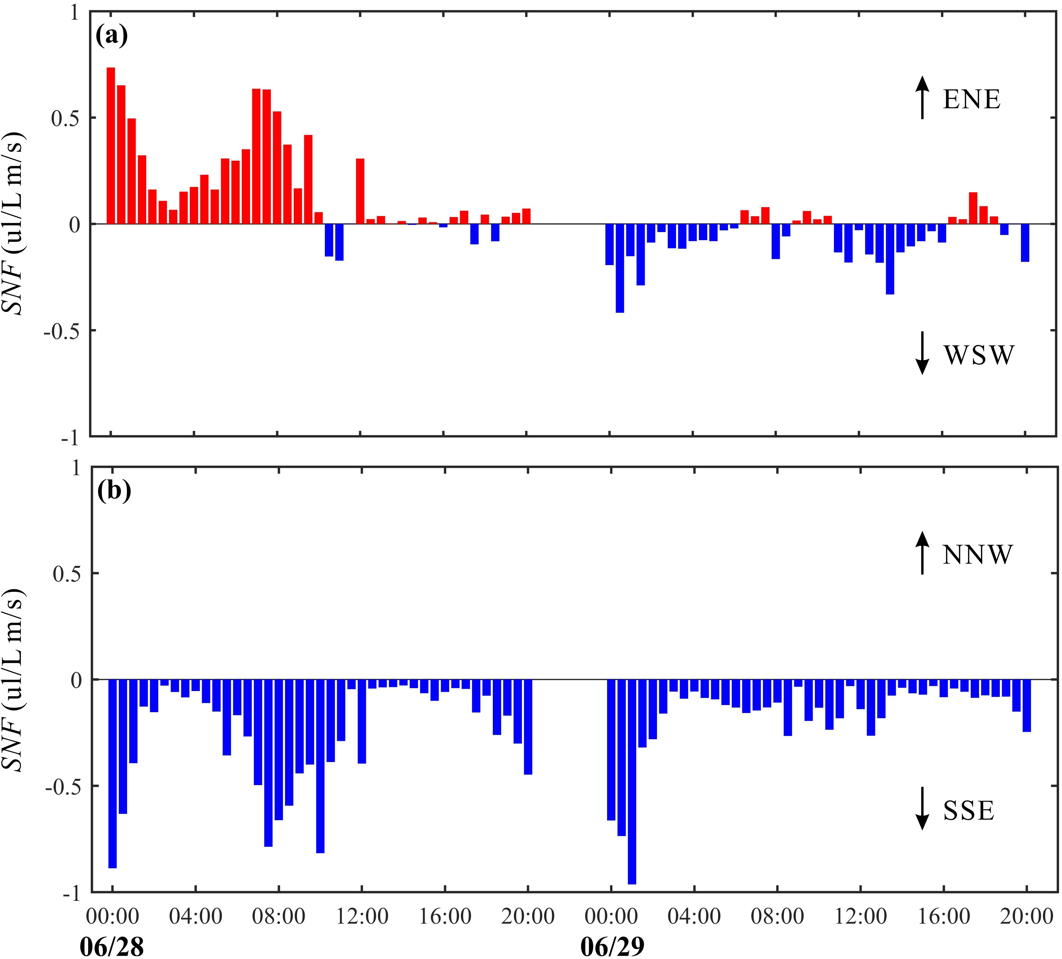
Figure 8. Time series of alongshore (a) and cross-shore (b) $SNF$ at Station (H) Positive values indicate ENE (NNW)-directed transport, while negative values denote WSW (SSE)-directed transport, arrows represent transport direction.

Our analysis reveals that the net sediment transport during the observation period was directed predominantly offshore and alongshore (Figure 8). The cross-shore component of the transport remained persistently offshore throughout the measurement period, even during the flood tide when the mean current was directed onshore. This counterintuitive result warrants further discussion.

This persistent offshore transport is likely driven by wave-induced undertow. In the nearshore and intertidal zone, the onshore mass transport of water by waves in the upper water column must be balanced by an offshore-directed return flow, known as undertow, near the bed (Longuet-Higgins, 1953). During our observation, moderate wave conditions were persistent. This undertow, a non-oscillatory current, superimposes on the tidal current. Even when the flood tide creates a net onshore flow, the near-bed undertow can be strong enough to ensure that sediment, once suspended, experiences a net offshore displacement. This mechanism is a well-documented driver of offshore sediment transport and beach erosion (Gallagher et al., 1998). The implication for Haiyang Beach is that even under fair-weather wave conditions, there is a persistent mechanism for offshore sediment loss from the intertidal flat, which could contribute to long-term erosional trends if not balanced by other processes (e.g., onshore transport during storms or calm periods).

The alongshore transport was strongly correlated with the tidal current direction, being southeastward during the ebb tide and northwestward during the flood tide, with the ebb-dominated transport resulting in a net southeastward flux. This directly identifying that the net transport is a product of both wave-induced processes (offshore undertow) and tidal asymmetry (net alongshore transport). This complex interaction underscores the necessity of considering both waves and tides to understand the sediment budget of mixed-energy intertidal systems.

4 Conclusions

This study provided an assessment of the mechanisms governing sediment dynamics in a mixed-energy, macrotidal intertidal environment, based on high-resolution in-situ observations. By decomposing the hydrodynamic forces into wave, current, and turbulence components, we have drawn several key conclusions that refine our understanding of such systems:

Sediment resuspension is dominated by near-bed turbulence. Multiple linear regression analysis demonstrated that turbulent was the primary and only statistically significant predictor of suspended sediment volume concentration ($TVC$). The direct influence of wave-induced bottom shear stress was negligible during the observed non-storm conditions. This finding highlights that the principal role of strong tidal currents in this environment is the generation of sediment-entraining turbulence, rather than direct bed erosion.

Net sediment transport is decoupled from wave direction and governed by subtidal currents. Despite the persistent onshore propagation of waves, the tidally-averaged net sediment transport was consistently directed offshore. This transport was controlled by the low-frequency subtidal flow, which represents a combination of ebb-dominant tidal residuals and wind-driven currents.

The interplay of hydrodynamics and sediment transport has clear morphodynamic implications. The persistent offshore export of sediment suggests that the intertidal zone at Haiyang is subject to chronic erosional pressure. Under typical weather conditions, the system acts as a conduit for sediment loss from the beach profile. This implies that the beach’s stability likely depends on sediment input from infrequent, high-energy storm events, a critical consideration for long-term coastal management and morphodynamic modeling.

While this study provides a detailed mechanistic understanding, its findings are based on single-point measurements. Future work should focus on deploying vertical arrays to resolve the boundary layer structure and employing spatial surveys to understand the broader morphodynamic context. Long-term monitoring is essential to capture seasonal variability and the crucial impact of storm events, which are necessary to build a complete picture of the annual sediment budget.

Data availability statement

The original contributions presented in the study are included in the article/supplementary material. Further inquiries can be directed to the corresponding author.

Author contributions

YY: Conceptualization, Formal analysis, Funding acquisition, Investigation, Methodology, Software, Validation, Visualization, Writing – original draft, Writing – review & editing. HS: Formal analysis, Investigation, Methodology, Software, Validation, Visualization, Writing – original draft, Writing – review & editing. XL: Formal analysis, Investigation, Software, Visualization, Writing – original draft, Writing – review & editing. LQ: Conceptualization, Data curation, Funding acquisition, Methodology, Project administration, Resources, Supervision, Validation, Writing – review & editing. YW: Conceptualization, Data curation, Funding acquisition, Methodology, Project administration, Resources, Supervision, Validation, Writing – review & editing.

Funding

The author(s) declare financial support was received for the research and/or publication of this article. This research was funded by the Youth Marine Science Fund of East China Sea Bureau, Ministry of Natural Resources (grant number 2024190303), and by the Fund of Fujian Key Laboratory of Island Monitoring and Ecological Development (grant number 2024ZD12).

Acknowledgments

The authors are grateful to the reviewers for their constructive comments.

Conflict of interest

The authors declare that the research was conducted in the absence of any commercial or financial relationships that could be construed as a potential conflict of interest.

The reviewer FG declared a past co-authorship with the author(s) XL to the handling editor.

Generative AI statement

The author(s) declare that no Generative AI was used in the creation of this manuscript.

Any alternative text (alt text) provided alongside figures in this article has been generated by Frontiers with the support of artificial intelligence and reasonable efforts have been made to ensure accuracy, including review by the authors wherever possible. If you identify any issues, please contact us.

Publisher’s note

All claims expressed in this article are solely those of the authors and do not necessarily represent those of their affiliated organizations, or those of the publisher, the editors and the reviewers. Any product that may be evaluated in this article, or claim that may be made by its manufacturer, is not guaranteed or endorsed by the publisher.

References

Barbier E. B., Hacker S. D., Kennedy C., Koch E. W., Stier A. C., and Silliman B. R. (2011). The value of estuarine and coastal ecosystem services. Ecol. Monogr. 81, 169–193. doi: 10.1890/10-1510.1

Crossref Full Text | Google Scholar

Bian C., Liu Z., Huang Y., Zhao L., and Jiang W. (2018). On estimating turbulent reynolds stress in wavy aquatic environment. J. Geophysical Research: Oceans 123, 3060–3071. doi: 10.1002/2017JC013230

Crossref Full Text | Google Scholar

Brand E., Chen M., and Montreuil A.-L. (2020). Optimizing measurements of sediment transport in the intertidal zone. Earth-Science Rev. 200, 103029. doi: 10.1016/j.earscirev.2019.103029

Crossref Full Text | Google Scholar

Brand E., De Sloover L., De Wulf A., Montreuil A.-L., Vos S., and Chen M. (2019). Cross-shore suspended sediment transport in relation to topographic changes in the intertidal zone of a macro-tidal beach (Mariakerke, Belgium). J. Mar. Sci. Eng. 7, 172. doi: 10.3390/jmse7060172

Crossref Full Text | Google Scholar

Fan R., Wei H., Zhao L., Zhao W., Jiang C., and Nie H. (2019). Identify the impacts of waves and tides to coastal suspended sediment concentration based on high-frequency acoustic observations. Mar. Geology 408, 154–164. doi: 10.1016/j.margeo.2018.12.005

Crossref Full Text | Google Scholar

Fugate D. C. and Friedrichs C. T. (2002). Determining concentration and fall velocity of estuarine particle populations using ADV, OBS and LISST. Continental Shelf Res. 22, 1867–1886. doi: 10.1016/S0278-4343(02)00043-2

Crossref Full Text | Google Scholar

Gallagher E. L., Elgar S., and Guza R. T. (1998). Observations of sand bar evolution on a natural beach. J. Geophysical Research: Oceans 103, 3203–3215. doi: 10.1029/97JC02765

Crossref Full Text | Google Scholar

Goring Derek G. and Nikora Vladimir I. (2002). Despiking acoustic doppler velocimeter data. J. Hydraulic Eng. 128, 117–126. doi: 10.1061/(ASCE)0733-9429(2002)128:1(117)

Crossref Full Text | Google Scholar

Grant W. D. and Madsen O. S. (1979). Combined wave and current interaction with a rough bottom. J. Geophysical Research: Oceans 84, 1797–1808. doi: 10.1029/JC084iC04p01797

Crossref Full Text | Google Scholar

Green M. O. and Coco G. (2014). Review of wave-driven sediment resuspension and transport in estuaries. Rev. Geophysics 52, 77–117. doi: 10.1002/2013RG000437

Crossref Full Text | Google Scholar

Kim S. C., Friedrichs C. T., Maa J. P. Y., and Wright L. D. (2000). Estimating bottom stress in tidal boundary layer from acoustic doppler velocimeter data. J. Hydraulic Eng. 126, 399–406. doi: 10.1061/(ASCE)0733-9429(2000)126:6(399)

Crossref Full Text | Google Scholar

Kolmogorov A. N. (1968). Local Structure of Turbulence In An Incompressible Viscous Fluid At Very High Reynolds Numbers. Soviet Phys. Uspekhi 10, 734. doi: 10.1070/PU1968v010n06ABEH003710

Crossref Full Text | Google Scholar

Le Hir P., Roberts W., Cazaillet O., Christie M., Bassoullet P., and Bacher C. (2000). Characterization of intertidal flat hydrodynamics. Continental Shelf Res. 20, 1433–1459. doi: 10.1016/S0278-4343(00)00031-5

Crossref Full Text | Google Scholar

Li L., Ren Y., Wang X. H., and Xia Y. (2022). Sediment dynamics on a tidal flat in macro-tidal Hangzhou Bay during Typhoon Mitag. Continental Shelf Res. 237, 104684. doi: 10.1016/j.csr.2022.104684

Crossref Full Text | Google Scholar

Liu X., Zhang H., Zheng J., Guo L., Jia Y., Bian C., et al. (2020). Critical role of wave–seabed interactions in the extensive erosion of Yellow River estuarine sediments. Mar. Geology 426, 106208. doi: 10.1016/j.margeo.2020.106208

Crossref Full Text | Google Scholar

Longuet-Higgins M. S. (1953). Mass transport in water waves. Philos. Trans. R. Soc. London. Ser. A Math. Phys. Sci. 245, 535–581. doi: 10.1098/rsta.1953.0006

Crossref Full Text | Google Scholar

Meng L., Tu J., Wu X., Lou S., Cheng J., Chalov S., et al. (2024). Wave, flow, and suspended sediment dynamics under strong winds on a tidal beach. Estuarine Coast. Shelf Sci. 303, 108799. doi: 10.1016/j.ecss.2024.108799

Crossref Full Text | Google Scholar

Niu J., Xie J., Lin S., Lin P., Gao F., Zhang J., et al. (2023a). Importance of bed liquefaction-induced erosion during the winter wind storm in the yellow river delta, China. J. Geophysical Research: Oceans 128, e2022JC019256. doi: 10.1029/2022JC019256

Crossref Full Text | Google Scholar

Niu J., Xie J., Zhou Y., Cai S., Dong P., Lin S., et al. (2023b). Wave-supported fluid mud and sediment vertical mixing under winter storm. Appl. Ocean Res. 141, 103768. doi: 10.1016/j.apor.2023.103768

Crossref Full Text | Google Scholar

Ren Z., Hu R., Zhang L., Wang N., and Zhu L. (2016). Evolution of the sandy beach in Haiyang. Mar. Geology Front. 32, 18–25. (in Chinese with English abstract). doi: 10.16028/j.1009-2722.2016.11003

Crossref Full Text | Google Scholar

Sun H., Xu J., Zhang S., Li G., Liu S., Qiao L., et al. (2022). Field observations of seabed scour dynamics in front of a seawall during winter gales. Front. Mar. Sci. 9. doi: 10.3389/fmars.2022.1080578

Crossref Full Text | Google Scholar

Temmerman S., Meire P., Bouma T. J., Herman P. M. J., Ysebaert T., and De Vriend H. J. (2013). Ecosystem-based coastal defense in the face of global change. Nature 504, 79–83. doi: 10.1038/nature12859, PMID: 24305151

PubMed Abstract | Crossref Full Text | Google Scholar

Xie W., Wang X., Guo L., He Q., Dou S., and Yu X. (2021). Impacts of a storm on the erosion process of a tidal wetland in the Yellow River Delta. CATENA 205, 105461. doi: 10.1016/j.catena.2021.105461

Crossref Full Text | Google Scholar

Xiong J., You Z.-J., Li J., Gao S., Wang Q., and Wang Y. P. (2020). Variations of wave parameter statistics as influenced by water depth in coastal and inner shelf areas. Coast. Eng. 159, 103714. doi: 10.1016/j.coastaleng.2020.103714

Crossref Full Text | Google Scholar

Yang Y., Wang Y. P., Gao S., Wang X. H., Shi B. W., Zhou L., et al. (2016). Sediment resuspension in tidally dominated coastal environments: new insights into the threshold for initial movement. Ocean Dynamics 66, 401–417. doi: 10.1007/s10236-016-0930-6

Crossref Full Text | Google Scholar

Yu Y., Wang Y., Qiao L., Wang N., Li G., Tian Z., et al. (2022). Geomorphological response of sandy beach to tropical cyclones with different characteristics. Front. Mar. Sci. 9. doi: 10.3389/fmars.2022.1010523

Crossref Full Text | Google Scholar

Yu H., Xie W., Peng Z., Xu F., Sun J., and He Q. (2024). The impact of a storm on the microtidal flat in the Yellow River Delta. Estuarine Coast. Shelf Sci. 311, 108978. doi: 10.1016/j.ecss.2024.108978

Crossref Full Text | Google Scholar

Yuan Y., Wei H., Zhao L., and Cao Y. (2009). Implications of intermittent turbulent bursts for sediment resuspension in a coastal bottom boundary layer: A field study in the western Yellow Sea, China. Mar. Geology 263, 87–96. doi: 10.1016/j.margeo.2009.03.023

Crossref Full Text | Google Scholar

Zhang X., Tan X., Hu R., Zhu L., Wu C., and Yang Z. (2021). Using a transect-focused approach to interpret satellite images and analyze shoreline evolution in Haiyang Beach, China. Mar. Geology 438, 106526. doi: 10.1016/j.margeo.2021.106526

Crossref Full Text | Google Scholar

Zhang S., Zhang Y., Xu J., Guo L., Li G., Jia Y., et al. (2022). In situ observations of hydro-sediment dynamics on the abandoned Diaokou lobe of the Yellow River Delta: Erosion mechanism and rate. Estuarine Coast. Shelf Sci. 277, 108065. doi: 10.1016/j.ecss.2022.108065

Crossref Full Text | Google Scholar

Zhu Q., van Prooijen B. C., Wang Z. B., Ma Y. X., and Yang S. L. (2016). Bed shear stress estimation on an open intertidal flat using in situ measurements. Estuarine Coast. Shelf Sci. 182, 190–201. doi: 10.1016/j.ecss.2016.08.028

Crossref Full Text | Google Scholar