Abstract
Introduction:
Species distribution models (SDMs) are increasingly used in fisheries science to understand species’ spatial patterns and improve stock assessments.
Method:
This study developed SDMs for eulachon smelt (Thaleichthys pacificus), a threatened, demersal forage fish often caught as bycatch in the United States West Coast ocean shrimp trawl fishery. Using ten years of observer data (2012–2021, n=19,749 with 25.4% being zeros), the study assessed the influence of static (e.g., substrate) and dynamic (e.g., ocean temperature, currents) environmental variables on eulachon abundance.
Results:
The best-performing SDM included near-bottom temperature and current data, outperforming SDMs using only surface variables. Eulachon abundance peaked at ~150 m depth, especially over gravel substrates, and during nighttime. Although none of the SDM-based abundance indices significantly correlated with the Columbia River stock assessment index, bottom-based SDMs showed stronger alignment with the stock assessment (R=0.61, p=0.08 & R=0.62, p=0.07).
Discussion:
Management implications are significant. Rock habitats were associated with higher eulachon bycatch, and vessels can use bottom-typing tools to avoid them. Also, delaying the season opener could reduce bycatch, as eulachon catch was reduced by 0.0109 mt per trawl over the interquartile range of day of the year. These findings can inform Best Management Practices (BMPs), which have historically led to regulatory changes such as the adoption of excluder grates and LED lights. Overall, incorporating near-bottom oceanographic data greatly enhanced predictive performance, especially for demersal species like eulachon. These mechanistic SDMs can be projected forward, aiding future management amid changing ocean conditions. While some discrepancies remain, this approach offers promising insights for adaptive fishery management and conservation of imperiled species like eulachon.
1 Introduction
Species distribution modeling (SDM) is becoming increasingly important in both stock assessment and non-assessment components fisheries science (Laman et al., 2018; Pickens et al., 2021; Rodrigues et al., 2023). In non-assessment contexts, SDMs are used to better understand how species ranges and distributions shift in response to ocean conditions whether they be “normal” climactic variations or longer term climate change associated variations (Muhling et al., 2016; Barnett et al., 2021). While SDMs are not directly used in management, the insights they provide can lead to the development of Best Management Practices (BMPs) and inform adaptive management strategies over time. In assessment contexts, SDMs are increasingly used in both fisheries-dependent and independent time series to account for missing data or changing methodologies and to reduce variance in the indices (based on observations or catch of fish) used as stock assessment inputs (Thorson et al., 2015; Alvarez-Berastegui et al., 2016; Paradinas et al., 2023). Reducing variance improves the overall quality of stock assessment models by reducing uncertainty around the metrics often used to guide fisheries management decisions (Harwood and Stokes, 2003; Hilborn, 2007). SDMs can also serve as indices of abundance based solely on environmental variables, which can be a particularly valuable approach when direct sampling is limited or fisheries-dependent data are insufficient for generating traditional indices (Tolimieri et al., 2018; Reglero et al., 2019; Sagarese et al., 2021).
When building SDMs to be used as indices of abundance, two main categories of environmental data are typically considered: 1) static benthic variables (substrate type, rugosity etc.) and 2) dynamic oceanographic variables (Juan-Jordá et al., 2009; Young and Carr, 2015; Rubec et al., 2016). For both types, the spatial and temporal resolution of the data must be carefully considered (Scales et al., 2017; Núñez-Riboni et al., 2021). Static benthic variables are especially important for groundfish and other demersal species to define essential fish habitat (Rooper and Martin, 2009; Young et al., 2010). The primary consideration for these variables is spatial resolution. However, static variables offer no insight into interannual variation in abundance or habitat conditions. In contrast, dynamic oceanographic variables, such as temperature, salinity, and current speed, can capture both direct and indirect drivers of annual variability in fish distributions (Keyl and Wolff, 2008). These data vary widely across both spatial and temporal scales and must be selected accordingly. One often-overlooked factor in oceanographic modeling is the vertical depth at which data are collected. Despite the fact that many species reside at depth, many SDMs rely solely on surface data, even though research has shown the added value of incorporating subsurface oceanographic information (Goetsch et al., 2023). While surface data often come from direct observation, benthic and deep oceanographic variables are increasingly available from high-resolution circulation models that are showing growing skill in SDM applications (Becker et al., 2016).
Eulachon smelt (Thaleichthys pacificus) are an imperiled anadromous Osmerid endemic to the nearshore shelf of the Northeast Pacific, returning to spawn in rivers and streams along the Pacific Northwest (PNW). Eulachon were first listed as “Threatened” under the Endangered Species Act (ESA) in 2010. Habitat loss, climate change, and fishery bycatch were identified as key threats to recovery (National Marine Fisheries Service, 2017). Eulachon live relatively short lives (2–5 years), are semelparous, and return to PNW rivers and streams between December and June each year. Eulachon spawning run timing is principally in the winter, generally before the spring outmigration period for juvenile salmon and steelhead, as well as before the adult spring salmon runs begin. Spawn timing combined with their high oil content made them a critical food source to indigenous tribes (Patton et al., 2019). Adult eulachon are also an important prey source for numerous marine animals including mammals (pinnipeds and whales), birds (gulls, ducks and eagles) and fish (salmon, sharks, halibut, hake, sablefish and rockfish) (National Marine Fisheries Service, 2017). Work has shown that historically eulachon were the most important component part of salmon diets when their population was large, however, given their threatened status Chinook salmon (Oncorhynchus tshawytscha) and Coho salmon (O. kisutch) have had to switch to primarily feeding on Pacific herring (Clupea pallasii) (Osgood et al., 2016). Beyond this, the relative importance of eulachon as compared to other species is not documented. The natural history of eulachon during spawning is well described; however, less is known regarding their natural history in the open ocean (National Marine Fisheries Service, 2017). Trophic studies in the ocean suggest that cumaceans and other benthic crustaceans make up an essential component of the diet of eulachon (reviewed in Gustafson et al., 2010). The vertical habitat of eulachon in the ocean is debated with certain sources claiming the fish are pelagic (Gustafson et al., 2010) whereas others claim they are benthic (Love, 2011). They are known to co-occur with ocean shrimp (Pandalus jordani) on the sandy/muddy habitats of the nearshore shelf where eulachon has been a historically common bycatch for the fishery targeting ocean shrimp (Hannah et al., 2018). Due to the paucity of information available about eulachon presence in the open ocean, the best available index of abundance for eulachon in the marine environment is derived from observer coverage data collected during the ocean shrimp fishing season.
The ocean shrimp, the target of the United States (US) West Coast’s second most valuable trawl fishery, is sustainably managed, through rigorous research, biological sampling, and regulation implementation around bycatch reduction (Hanna et al., 2022). Each of the US West Coast states (California, Oregon, and Washington) that manage ocean shrimp fisheries work together to align regulations and address issues. Ocean shrimp are valued at 33.2 million USD and have landings 26,540 mt (2012-2021), annually. Oregon’s ocean shrimp fishery was the first to be certified sustainable by the Marine Stewardship Council (MSC) in 2007, followed by Washington (2015), then California (2022). Fishery landings have historically occurred primarily in Oregon, with 72.8% of US West Coast landings (2011-2024), followed by Washington (20.8%) and California (6.4%) (https://pacfin.psmfc.org/). The Oregon ocean fishery annual season begins April 1st, and closes October 31st. The gear employed are primarily double rigged trawls that fish off the muddy/sandy bottoms at depths from 73 m to 274 m. Since ocean shrimp are small, reaching maximum weights of 10–12 grams (Groth, 2018), fine mesh nets with openings of 30–38 mm (Bancroft and Groth, 2021) are employed, and as such, bycatch was relatively high (Hannah and Jones, 2007). Two major innovations in bycatch reduction have dramatically reduced overall bycatch, 1) in 2012–19 mm spaced rigid aluminum Nordmøre grates (BRD), were required to be placed between the net and codend to physically eliminate most fishes and 2) in 2018 five LED fishing lights were required to be placed on the footrope which encourage fish behaviors that avoid entrainment (https://secure.sos.state.or.us/oard/viewSingleRule.action?ruleVrsnRsn=241299). Together, the two bycatch reduction devices keep bycatch rates consistently less than 5% of total (Groth, 2020). Annual bycatch rates for eulachon in the ocean shrimp fishery are calculated through data collected by observers in the West Coast Groundfish Observer Program (WCGOP) (https://www.fisheries.noaa.gov/west-coast/fisheries-observers/northwest-fisheries-science-center-observer-programs). Observers collected fishery dependent data on all non-target species caught during ocean shrimp vessel trips, covering 30-40% of trips annually through 2024. Changes to the WCGOP suspended observer coverage of the ocean shrimp fishery taking effect in January 2025. Modern ocean shrimp trawl nets have been specifically engineered to minimize bycatch of eulachon smelt, given their status. Research has shown that the use of “eulachon optimized” grid spacing (19.1 mm) reduces eulachon catch by 16.6% when compared to 25mm spacing (Hannah et al., 2011), and use of LED fishing lights reduces bycatch dramatically further (70-91%) (Hannah et al., 2015; Lomeli et al., 2018). From 2012 to 2021, eulachon have been 74.6% of ocean shrimp bycatch (average 17 ± 46 kg per haul). Despite the massive reduction of bycatch rates for eulachon smelt in the ocean shrimp fishery, its scale is worth consideration in relation to the imperilment of eulachon. While bycatch from the ocean shrimp fishery is unlikely to have population level impacts (Hannah, 2014), reducing bycatch without substantial reductions in shrimp catch is obviously desirable for both the industry and conservation interests.
Management of eulachon is challenged by a paucity of data, highlighted by gaps in understanding regarding spawning run timing, size, and location. Additionally, there is limited understanding about the population dynamics of this species once they enter the ocean and prior to return to their spawning grounds in West Coast rivers and estuaries of the United States (Anderson, 2022). The greatest threat to their recovery are altered ocean and freshwater conditions due to changes in climate (Anderson, 2022), yet there is relatively little known about how changing ocean climate conditions will affect eulachon in the marine environment. SDMs could be valuable tools to enhance the availability of information about eulachon populations in the ocean and may provide an important potential analytical framework to better manage eulachon recovery and foster a sustainable ocean shrimp trawl fisheries on the West Coast of the United States.
The California Current is a monsoonal upwelling system that originates near 49° N, where the west wind drift collides with Vancouver Island and turns south (Hickey, 1979; Checkley and Barth, 2009). As an eastern boundary current, it is broad (~500 km) and relatively slow (0.1–0.25 m s⁻¹). During winter, a northward-flowing current known as the Davidson Current develops over the continental shelf. In spring, following an approximately seven-day period referred to as the spring transition, the flow shifts to the southward-moving California Current, which extends both on and off the continental shelf (Huyer et al., 1979; Strub et al., 1987). In summer, strong northerly winds drive offshore transport of surface waters via Ekman processes. In response, deeper waters are advected shoreward and upward, bringing cold, nutrient-rich water onto the shelf and to the surface. When these winds weaken or cease, warmer offshore surface waters flow back toward the coast, while the colder near-bottom waters are advected offshore. Throughout this period, the net transport remains southward. To support ongoing monitoring and bycatch mitigation, we developed SDMs using 10 years of at sea observer data from NOAA’s West Coast Groundfish Observer Program. These SDMs aim to understand how both static and dynamic environmental variables influence the predicted abundance of eulachon in the ocean shrimp fishing grounds. Conducting this study from an applied management perspective for a threatened marine species provides information to evaluate the utility of SDMs to enhance management decisions for data limited recreational and commercial eulachon fisheries.
2 Materials and methods
2.1 Fisheries data
We used Eulachon data were obtained from the NOAA Fisheries observer program from observers deployed on vessels targeting ocean shrimp (Pandalus jordani).Only data from the California Current were used (bounded by 48°N to 39°N). Observed vessel trips were subsampled by using a stratified random design developed by NOAA. Approximately 80,000 trips targeting ocean shrimp occurred from 2011–2024 and ~30% of trips were sampled, stratified by port group and month. Data from the trips were processed and expanded to estimate take of entire fishery. Observers estimated biomass of eulachon for each tow. Observer data were filtered to only include data from 2012–2021 based on availability of the environmental covariates used for modeling. In this study, 19,749 trawls were included in the analysis of which 5,013 did not capture eulachon (Figure 1).
Figure 1
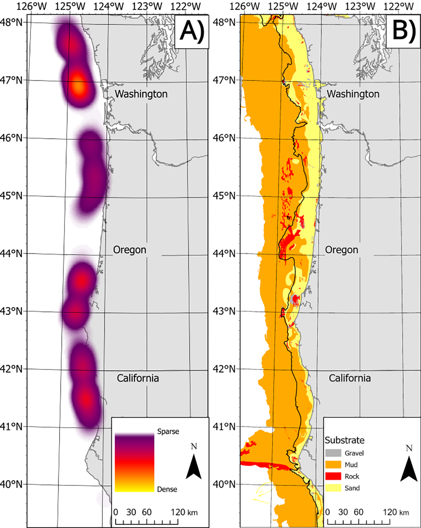
(A) heat map of shrimp trawls from 2012-2021. Data are shown in aggregate to meet data privacy laws. (B) Map of benthic habitats (colors) and 200 m contour). .
2.2 Model covariates
2.2.1 Observer derived
For each tow, we used the date and time of net deployment to determine the hour of the day (rounded to the 10th of an hour) and the day of the year (Table 1). Since BRDs were mandated by law for the entirety of our modeled time series they were not included as a covariate. However, LEDs were not required until 2018 so their presence/absence was also included as a binomial covariate in the SDM. A vessel identifier was also included as a random effect in the models. Finally, the year was included in the SDM as well. Shrimp biomass was not included as a covariate in the model because we wanted to be able to predict eulachon abundance and observer coverage of the fishery has been cancelled.
Table 1
| Variable | Abbreviation | Units | Source | SDMs Using | Spatial resolution | Temporal resolution | Minimum | Maximum | Mean |
|---|---|---|---|---|---|---|---|---|---|
| Log10 Depth | Log10(depth) | Meters | DEM | All | 50 m x 50 m | ― | 32.75 (1.51) | 229.27(2.36) | 132.01(2.12) |
| Hour of Day | HR | Hour | Observer | All | ― | Tenth of hour | 0.00 | 23.00 | 15.06 |
| Day of Year | DOY | Day | Observer | All | ― | Day of Year | 91.00 | 303.00 | 198.20 |
| LED Lights Present | LED | +/- | Observer | All | ― | ― | ― | ― | ― |
| Fishing Vessel Identifier | VESSEL | +/- | Observer | All | ― | ― | ― | ― | ― |
| Year | year | Year | Observer | All | ― | Year | 2012 | 2021 | 2016 |
| Substrate | substrate | Categorical | sghV4 | All | 100 m x 100 m | ― | ― | ― | ― |
| Sea Surface Temperature | SST | °C | ROMS | Equation 2, Equation 4, Equation 6 | 0.1° x 0.1° | Daily | 7.72 | 20.00 | 13.37 |
| Surface alongshore velocities | SSV | m s-1 | ROMS | Equation 4, Equation 6 | 0.1° x 0.1° | Daily | -0.93 | 0.57 | -0.14 |
| Surface cross-shelf velocities | SSU | m s-1 | ROMS | Equation 4, Equation 6 | 0.1° x 0.1° | Daily | -0.75 | 0.39 | -0.02 |
| Chlorophyll | chl | mg m-3 | MODIS | Equation 6 | 4 km x 4 km | 7 Day Average | 0.01 | 429.12 | 5.10 |
| Temperature Fronts | fronts | °C km-1 | MUR | Equation 6 | 0.01° x 0.01° | Daily | 0.00 | 0.93 | 0.23 |
| Bottom temperature | bot_temp | °C | ROMS | Equation 3, Equation 5 | 0.1° x 0.1° | Daily | 1.84 | 9.68 | 6.65 |
| Bottom alongshore velocities | bot_V | m s-1 | ROMS | Equation 5 | 0.1° x 0.1° | Daily | -0.43 | 0.51 | 0.08 |
| Bottom cross-shelf velocities | bot_U | m s-1 | ROMS | Equation 5 | 0.1° x 0.1° | Daily | -0.46 | 0.29 | -0.03 |
Variables considered in the SDMs.
All variables were modeled in their raw form (not centered or scaled) except for depth which was log10 transformed to reduce skew. For alongshore velocities, positive values denote currents flowing to the north and negative currents flowing to the south. For cross-shelf velocities, positive values denote currents flowing to the east (toward shore) and negative values denote currents flowing to the west (offshore). Parentheses of values for Log10 depth denote the log transformed values. DEM denotes the digitized NOAA charts referenced in section 2.2.3.
2.2.2 Non-oceanographic data
National Oceanic and Atmospheric Administration paper navigation charts were digitized into Electronic Navigation Charts (ENC’s). The depth soundings were collated into a “Digital” collection (shapefile) in ArcGIS Pro. These data were converted into a raster and depth was extracted on a 50 x 50 m grid. To increase the spatial resolution, we used generalized additive models in the mgcv R package to interpolate depths onto a finer mesh (Wood, 2011). We first fit a simple generalized additive model with depth as the explanatory variable and a latitude longitude tensor interaction. Data were modeled using a normal distribution (R2-adj = 0.919, RMSE = 60.74). We then predicted the depth at which each individual trawl was deployed. This model-based approach was validated by fitting a linear relationship between depths reported by the observers (generated from the vessel’s echosounder) and modeled depths generated by the afore mentioned generalized additive model (R2 = 0.90).
We also used benthic habitat data from the Surficial Geologic Habitat (sghV4) layer produced by the Bureau of Ocean Energy Management (BOEM) (Goldfinger et al., 2014). Data were from the Lith3 category were simplified into four categories (sand-22% of data, mud- 72% of data, gravel-2% of data and hard-4% of data- Figure 1). See Rasmuson et al. (2022) for a description of what categories were aggregated into each of the four larger categories. Shortly, Lith3 is the highest resolution benthic geological habitat divided into 42 categories based on a combination of multiple empirical methods (Goldfinger et al., 2014).
2.2.3 Oceanographic data
Sea surface temperature and ocean current data were obtained from a regional ocean circulation model (Table 1). Ocean velocities were provided by a data assimilative ocean circulation model developed using the Regional Ocean Modeling System (ROMS). This 1/10 degree, realistic California Current implementation is based on the forward model configuration of Veneziani et al. (2009), which accurately represents seasonal and mesoscale processes in the California Current. Historical analyses are based on a 4-Dimensional Variational Assimilation algorithm (Broquet et al., 2009; Moore et al., 2011; Edwards et al., 2015) in which ocean state estimates are constrained by observations of sea surface height, sea surface temperature, in situ observations of temperature and salinity from gliders, and surface velocity estimates from high frequency radar. Daily model output is saved from four-day assimilation cycles (Moore et al., 2013). No tidal motion or Stokes’ drift associated with surface waves were included in this analysis. Given this, the model is best able to resolved mesoscale processes and not others that occur at smaller spatial or temporal scaled. For each trawl location, the associate temperature at the surface and bottom as well as alongshore and cross-shelf components of velocity were extracted. At 100 m depth the surface layer is 0.28 m thick and at the bottom 5.7 m thick. On average the change in depth between adjacent grid cells, in the cross shelf direction, is 5.2 ± 6.4 m. Metrics were extracted by selecting the ROMs grid cell which contained the trawl at the time step closest to when the middle of the trawl was occurring. In other words no downscaling of the ROMs model occurred.
Remote-sensed data were obtained for sea surface fronts and chlorophyll-a (Table 1). Surface fronts were identified using the daily MUR SST v4.1 frontal edge dataset. (https://upwell.pfeg.noaa.gov/erddap/griddap/erdMurFront41USWest.html). The frontal index value was extracted for the day and location at which each trawl was deployed. Daily chlorophyll-a data were obtained from the science quality 4 km Aqua MODIS programs sensor (https://upwell.pfeg.noaa.gov/erddap/griddap/erdMH1chla1day.html). For each trawl location, we manually calculated a seven-day average of chlorophyll-a, with the final value being the day of the trawl and the other values being the six preceding days.
2.2.4 Covariate preprocessing
Prior to beginning model fitting, we followed Zuur et al. (2010) to ensure that all variables were not collinear and other essential assumptions were met. Analyses were restricted to the time of the year when the shrimp fishery is open (April 1st – October 31st). We also restricted analysis to 2011–2021 based on this being the availability of environmental covariates. Depth data were log10 transformed to reduce skew. All other covariates did not require scaling and centering prior to fitting. After the SDM were established, they were run a second time with scaled and centered data. Fits did not improve and thus untransformed data were used to improve in interpretation.
2.3 SDM algorithm overview
We fit our SDMs using a generalized mixed effects modeling approach in the sdmTMB package (Anderson et al., 2022). The SDM uses Stochastic Partial Differential Equation (SPDE) and the Integrated Nested Laplace aApproximation (INLA) to handle the large amount of data being used (Lindgren et al., 2011; Martino and Riebler, 2019). The SDM is effectively a generalized mixed effects model that can also include spatial and spatiotemporal random fields. The covariates are often modeled as linear effects though they can also be modeled in a non-linear fashion, similar to generalized additive models. The random fields allow the SDM to capture variation not explained by the covariates included in the SDM. These may represent truly random processes or those could be explained by additional covariates not yet included.
2.4 SDM implementation
All SDMs considered were modeled using a Tweedie distribution and a log link. A comparison to delta-gamma is included in the online supplement Supplementary Table S1. SDMs were with spatiotemporal random fields but not temporal autocorrelation. No temporal autocorrelation was included in the SDMs because time was modeled explicitly. The mesh included 1,947 knots and no barrier mesh was included. Anisotropy was included in the model and no priors included during the fitting. We compared six a priori SDMs of varying complexity using environmental data from different parts of the water column. All continuous variables not modeled as interactions were treated as non-linear variables and restricted to five knots to prevent overfitting and ensure that trends were ecologically interpretable (Pedersen et al., 2019; Asch et al., 2022). All SDMs included the following variables:
Where Eulachon_mt is the metric tons of eulachon caught in a given tow, s denotes variables modeled using a smooth (penalized splines, which again were restricted to 5 knots), cc denotes a variable modeled with a cyclic smooth function, DOY denotes day of the year, HR denotes the hour of the day in 10ths of an hour, depth denotes sea floor depth where the tow was conducted and log10 transposed to reduce skew, substrate is a categorical variable of habitat type on the bottom, year indicates the year the tow was conducted, re(LED) is a random effect denoting the presence or absence of LED lights in the nets, re(VESSEL) denotes a random effect for vessel identifier, offset denotes the presence of an offset term modeled as log length of the tow in minutes. For simplicity, when showing the structure of the SDMs we will just include a term base which indicates the structure shown in Equation 1.
Two of the SDMs only included a measure of temperature as an environmental covariate (Equations 2, 3):
Where SST is the sea surface temperature in °C at the location the tow was conducted, and bot_temp denotes the bottom temperature in °C at the location the tow was conducted. Two SDMs of increasing oceanographic complexity were also considered (Equations 4, 5):
Where SSU.SSV denotes an interaction between the cross-shelf and alongshore surface currents (both in m s-1) and bot_U and bot_V (both in m s-1) denotes an interaction between the cross-shelf and alongshore bottom currents. In the case of these interactions we did not restrict the k values due to the complexity of the interaction. The final SDM included remote sensed environmental metrics as a proxy for concentrating features and trophic conditions (Equation 6):
Where chl denotes the seven-day average chlorophyll at the location of the tow in mg m-3. fronts denotes the maximum horizontal frontal gradient in °C km-1 at the location of the tow.
2.5 SDM evaluation
For each SDM, we first ensured a good model fit by using the “sanity” check in sdmTMB. Following this, residuals were examined using the dharma package (Hartig, 2024). To remove the assumption that the spatiotemporal random fields can be modeled using a multivariate normal distribution, we also resampled the random effects using Markov Chain Monte Carlo (MCMC) simulations. All SDMs passed these steps, allowing for continued comparison of the models. SDM fit was compared six different ways. First, we calculated the delta Akaike Information Criterion for small sample size (ΔAICc), Akaike weight, the Root Mean Square Error (RMSE) and Mean Absolute Error (MAE) for each of the six SDMs. ΔAICc and Akaike weight are used to compare and rank models based on their relative support from the data; models with lower ΔAICc values (typically <2) are considered to have substantial support. Akaike weights range from 0 to 1 and represent the relative likelihood of each model being the best among the set with values closer to 1 indicating stronger support. RMSE and MAE assess predictive accuracy by measuring the average magnitude of prediction errors, with lower values indicating better model performance.
We then used three different forms of k-fold validation. First, we ran 100 iterations of a five-fold cross-validation and compared the sum loglikelihood from these models. These folds were randomly selected in each iteration. Second, additional analysis was done using a k-folds analysis with each fold defined by a sampling year and we compared the sum log-likelihood from these analyses Finally, we used k-means to spatially block the data (4–10 blocks), ran a k-folds analysis with this blocking and compared the sum log-likelihood. Based on maximum sum log-likelihood across all SDMs, eight spatial blocks were the most supported blocking.
2.6 SDM predictions and indices
Daily predictions were generated from April 1 to October 31 for the years 2012 to 2021, from 48°N to 38°N and from the 200 m contour to the shore. Data were first extracted from the same regional ocean model used to generate the model fits (see section 2.2.3). Then using the centroid of each of these grid cells, the associated habitat, depth, seven-day mean chlorophyll and frontal gradient values were extracted from the same sources used for the SDM development. Using these data, predictions for each of the six SDMs were generated and then averaged into a single map of Eulachon habitat. An index of abundance was also generated for each of the six SDMs using the get_index function from sdmTMB. These data were compared to an estimated index of abundance for eulachon in the Columbia river (Joint Columbia River Management Staff, 2024) by calculating a Pearson’s correlation between the stock assessment index and each of the SDM generated indices independently. Prior to correlation analysis, all indices were z-score standardized to place them on a common scale with a mean of zero and standard deviation of one, which ensures comparability by removing differences in units and magnitude across datasets. Z-score standardization is performed by subtracting the mean of each index from individual values and then dividing by the standard deviation, allowing patterns in variability and correlation to be compared meaningfully across models.
3 Results
3.1 SDM comparison
The best fit SDM (Equation 5) was the SDM that included bottom temperature and the near-bottom current velocities (Table 2). The SDM was strongly supported by ΔAICc and Akaike weight. Measures of RMSE and MAE also indicated that Equation 5 was the best fit SDM, but the results were not as striking as those from the AIC based metrics. There was overlap in the sum log-likelihood values from the 100 iterations of 5 k-fold validation but the median for Equation 5 was higher than the other SDMs (Figure 2). However, of the six SDMs, Equation 5 had the largest spread in sum log-likelihood values. Using spatial blocking defined by k-means, eight blocks had the highest support overall and Equation 5 had the highest support, followed by Equation 3.
Table 2
| Model Equation | Tweedie distribution parameters | ΔAICc | Akaike weight | RMSE | MAE | Median sum log-likelihood ± standard deviation | Spatial blocking sum log-likelihood | Temporal sum log-likelihood |
|---|---|---|---|---|---|---|---|---|
| Equation 1 | p = 1.69 φ = 0.46 | 261.9 | 1.32 e-57 | 0.0390 | 0.0143 | 41,904 ± 151 | 11,321 | 28,170 |
| Equation 2 | p = 1.69 φ = 0.45 | 171.0 | 7.52 e-8 | 0.0427 | 0.0144 | 41,897 ± 229 | 11,321 | 28,170 |
| Equation 3 | p = 1.69 φ = 0.44 | 109.2 | 1.94 e-24 | 0.0414 | 0.0143 | 41,776 ± 351 | 12,110 | 29,289 |
| Equation 4 | p = 1.69 φ = 0.45 | 205.5 | 2.43 e-45 | 0.0405 | 0.0144 | 41,786 ± 408 | 11,251 | 27,792 |
| Equation 5 | p = 1.69 φ = 0.44 | 0 | 1.00 | 0.0389 | 0.0142 | 42,050 ± 352 | 12,247 | 30,426 |
| Equation 6 | p = 1.69 φ = 0.45 | 156.6 | 9.77 e-35 | 0.0391 | 0.0143 | 41,778 ± 634 | 11,263 | 28,167 |
Comparison of predictive abilities of the six a priori SDMs.
ΔAICc is the delta Akaike Information Criterion corrected for small sample size calculated by subtracting the AICc of each model from the best fit model, RMSE- Root Mean Square Error for each SDM, MAE- Mean Absolute Error for each SDM. Median Sum Log-likelihood is based on 100 iterations of randomly selected five folds k-validation for each SDM, Spatial Blocking Sum Log-likelihood is based on eight spatial blocks defined by k-means, Temporal blocking is based on a k-folds analysis with each year as a fold.
Figure 2
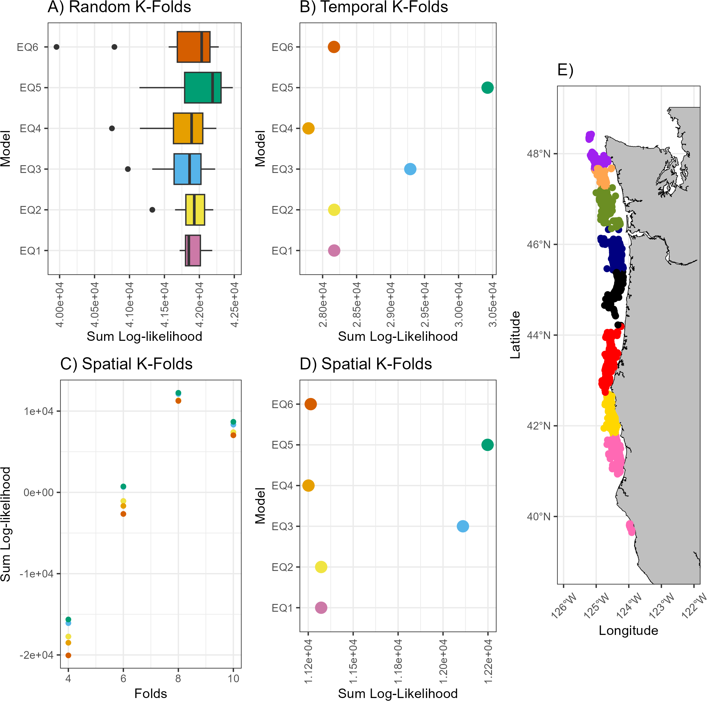
Comparison of the six a priori SDMs using 3 methods (A-Random, B-Temporal and C to E- Spatial) of k-folds cross validation. (C) show how the number of spatial folds differ in overall sum log-likelihood, (D) provides a close up of 8 folds (the best option per panel (C) and (E) shows the locations where the 8 folds were split. In all instances higher sum log-likelihood values indicate a better model. See section 2.5 for more information.
All fixed effects (year and substrate) were present in each of the six SDMs. The SDM trends were highly similar across all six SDMs (Online Supplementary Figures S1, S2), though the first two years had more variability than the remaining years. Due to the similarity we only present the plots derived from Equation 5. Eulachon abundance was highest in rock habitats, though high variance in abundance was also associated with this habitat type (Figure 3). Abundance of eulachon was highly variable between years with the highest year 2013 and the lowest being 2017 (Figure 4).
Figure 3
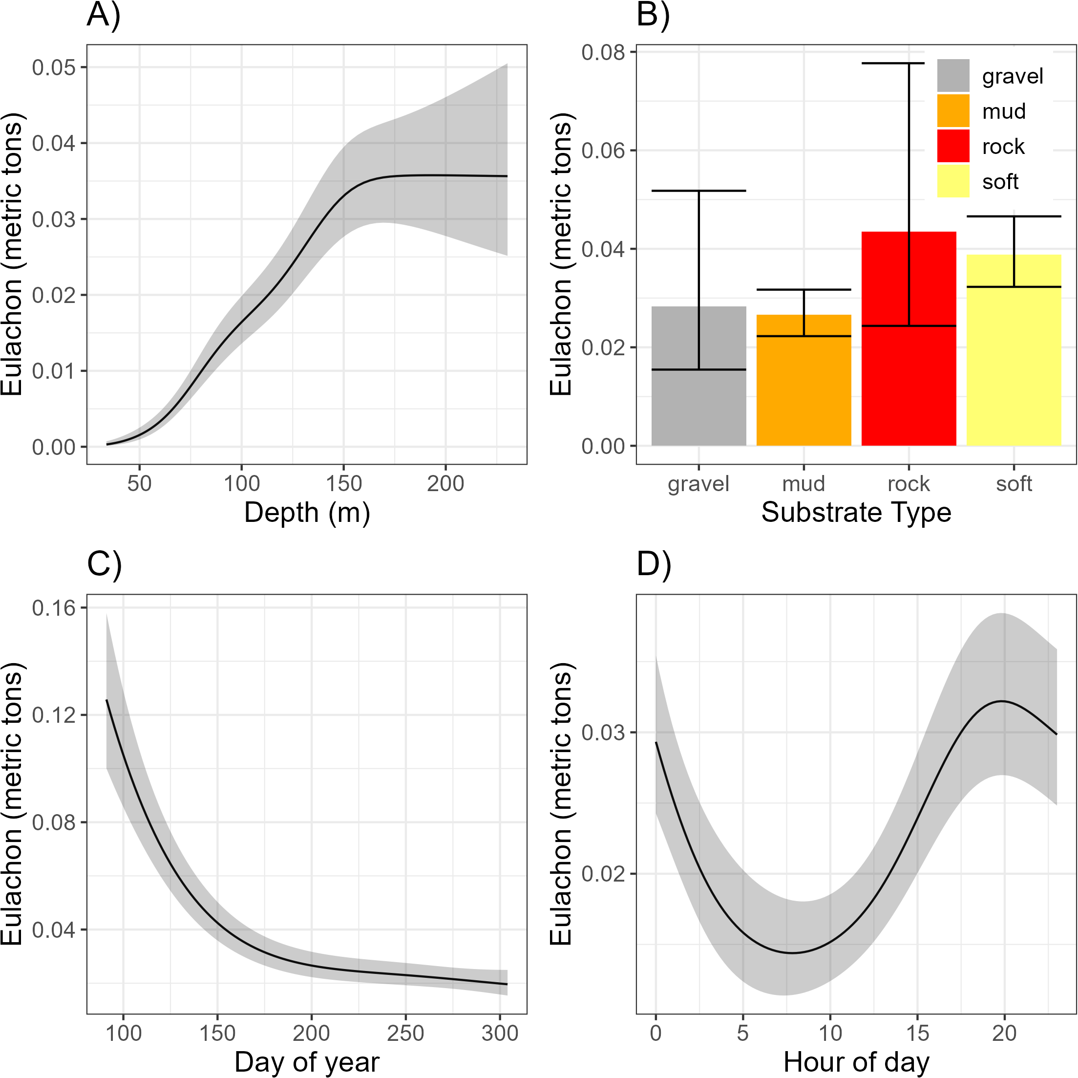
Affects of Depth (A), Substrate type (B), Day of year (C) and Hour of day (D) on the catch of eulachon. Results are from the top SDM (Equation 5). The trends were similar across all six SDMs.
Figure 4
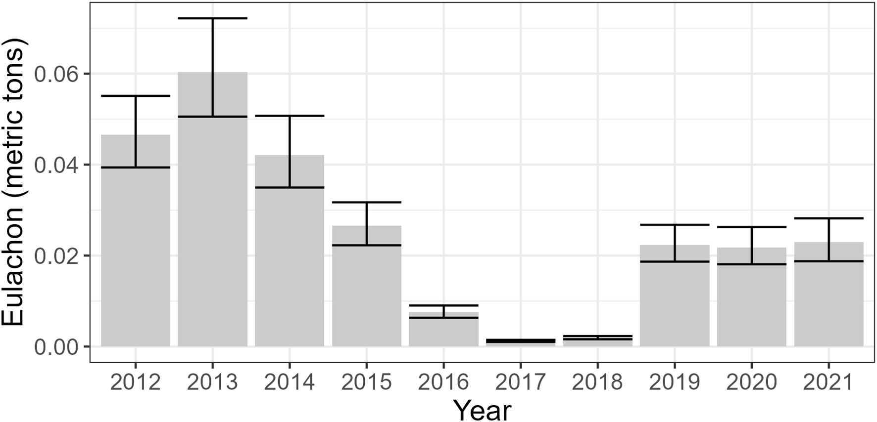
Effect of year on the catch of eulachon. Results are from the top SDM (Equation 5). The trends were similar across all six SDMs.
For the shared continuous effects (day of year, hour of day, and depth), the SDM smooth effects were similar among the six SDMs, with notable minor differences in day of the year (Figure 5). The trends in the smoothers were similar across all six SDMs, so only those from Equation 5 are presented. There was a significant decline in the abundance of eulachon as the fishing season progressed (Figure 3). Eulachon abundance peaked at a depth of ~150 m (which is where most shrimping occurs) and was also highest around 8:00 pm (local) each day.
Figure 5
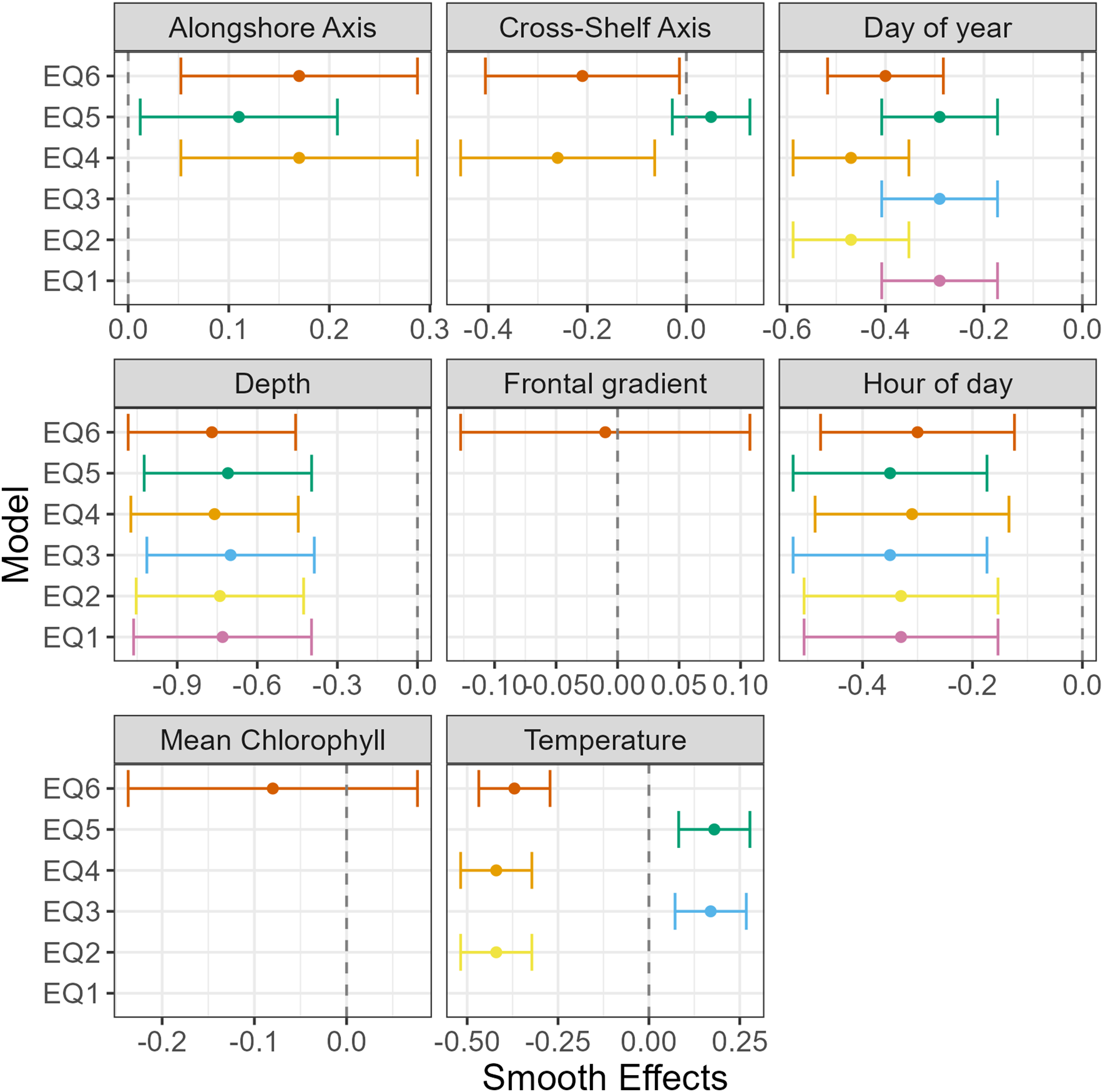
Smooth effects for the six a priori SDMs. Bars are mean ± 95% confidence intervals. EQ1, Equation 1; EQ2, Equation 2; EQ3, Equation 3; EQ4, Equation 4; EQ5, Equation 5; EQ6, Equation 6.
For temperature, the SDMs that included bottom temperature Equation 3 and Equation 5) had positive smooth effects whereas the SDMs with sea surface temperatures had negative smooth effects (Figure 5). When examining the relationship between eulachon abundance and temperature at each depth, the abundance of eulachon was more common in cooler temperature waters at the bottom and warmer temperatures at the surface (Figure 6). This pattern is maintained, but scales are different when the spatial random fields were turned off (Online Supplementary Figure S4).
Figure 6
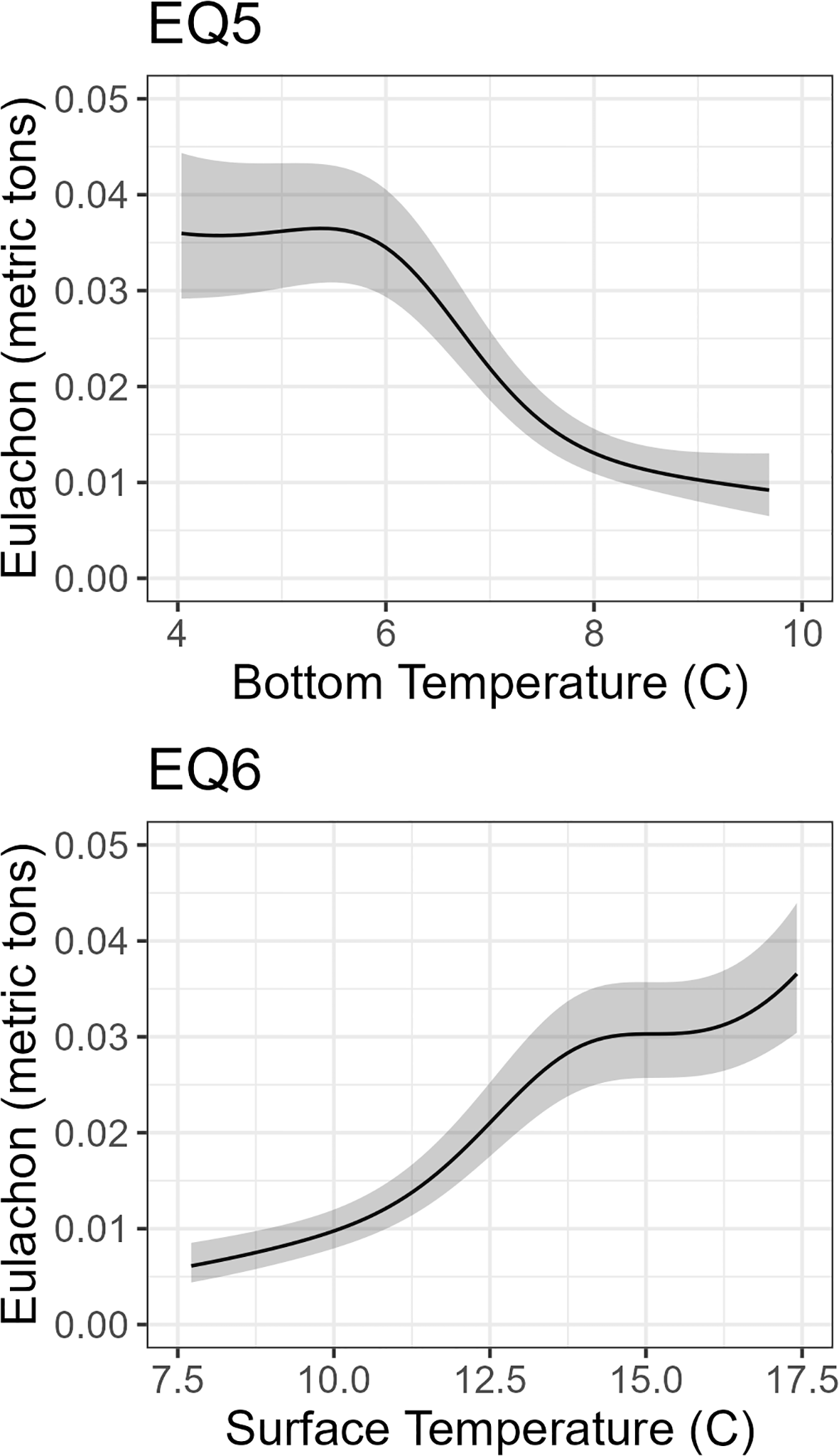
Affects of bottom temperature (Equation 5) and sea surface temperature (Equation 6) on the catch of eulachon. Results from bottom temperature are similar in Equation 3 and Equation 5. Results from sea surface temperature are similar in Equation 2, Equation 4 and Equation 6. EQ5, Equation 5; EQ6, Equation 6.
For currents, the alongshore currents had positive smooth effects though the surface currents had lower mean estimates (Figure 5). Similar to temperature, smooth effects for surface currents were negative and positive for near-bottom currents. At the bottom, eulachon abundance was highest when currents are to the south and offshore (Figure 7). At the surface, eulachon abundance was highest when surface currents were to the south but shoreward.
Figure 7
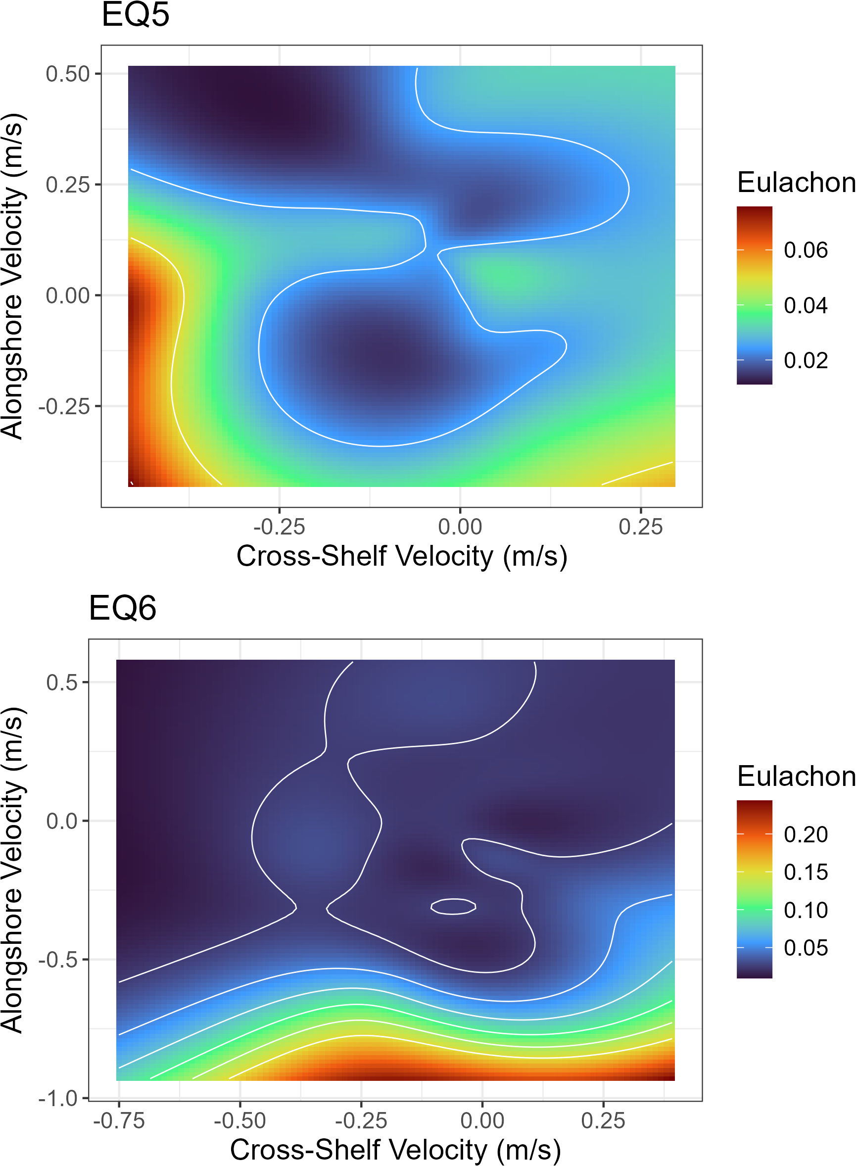
Smooth smoother interaction between alongshore and cross-shelf currents (near-bottom- top panel, surface- bottom panel) on the number of eulachon caught. Positive values on the x-axis denote currents flowing to the east (shoreward) and negative values denote currents flowing to the west (offshore). Positive values on the y-axis denote currents flowing to the north and negative values currents flowing to the south. Contours are presented at 0, 0.025, 0.05, 0.075, 0.10, 0.125 and 0.15 metric tons of eulachon. EQ5, Equation 5; EQ6, Equation 6.
3.2 SDM prediction and indices
Regardless of SDM structure, the SDMs all agreed that the offshore waters of Washington were not good eulachon habitat (Figure 8, uncertainty maps shown in Supplementary Figure S5 in Online Supplementary). The SDMs generated using surface oceanographic data generally showed more nearshore populations, whereas the near-bottom SDMs suggested more offshore populations. The SDM also increased its prediction of eulachon biomass offshore when including the near-bottom currents as a covariate. The striking differences in patterns observed between SDMs were reduced when spatial random fields were turned off (Online Supplementary Figures S6, S7).
Figure 8
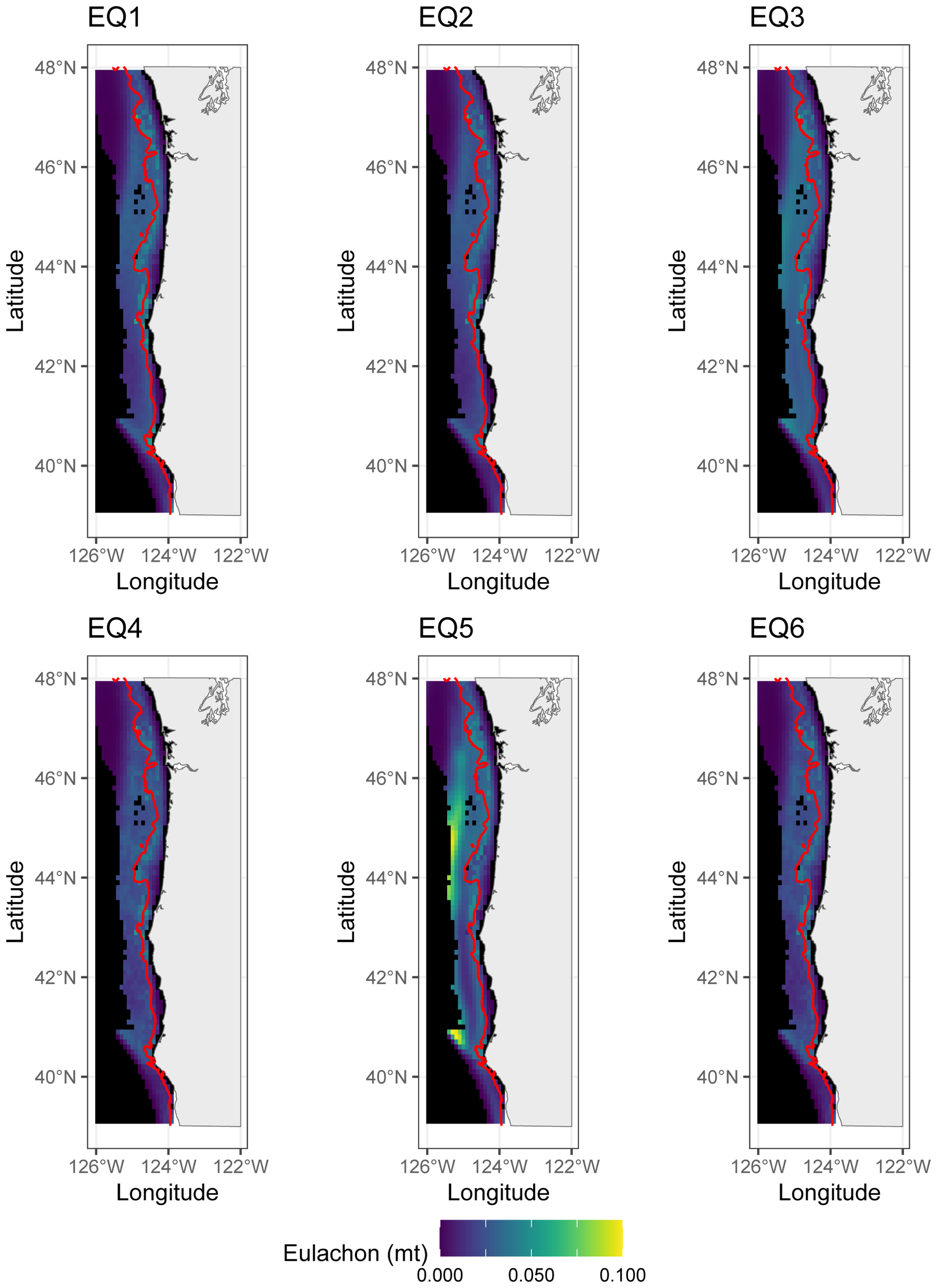
Predicted abundance of eulachon for each of the six a priori SDMs. Each SDM represents an average of all the years. All maps are plotted on the same color scale. The redline on the graph is the 200 m contour line. EQ1, Equation 1; EQ2, Equation 2; EQ3, Equation 3; EQ4, Equation 4; EQ5, Equation 5; EQ6, Equation 6.
Overall, the SDM indices share a generally consistent trend (Figure 9). However, when Z-score standardized, none of the correlations between our indices and the stock assessment were significant (Table 2). However, the near-bottom indices (Equation 3 and Equation 5) had large R values, and the p values were much closer to being defined as significant.
Figure 9
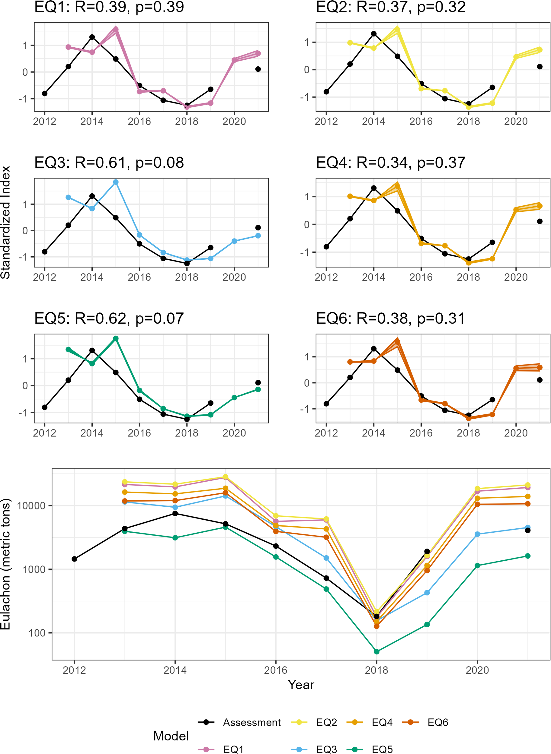
Indices of abundance from the SDMs (colored lines) versus the eulachon abundance predicted in the most recent eulachon stock assessment. Upper panels are z-score standardized and correlations are presented in the titles. None of the time series are significantly correlated with the stock assessment time series. Bottom plot shows the raw estimated biomass. Areas around lines denote 95% confidence intervals. Note some confidence bands are so small they are hard to see. EQ1, Equation 1; EQ2, Equation 2; EQ3, Equation 3; EQ4, Equation 4; EQ5, Equation 5; EQ6, Equation 6.
4 Discussion
Our SDM exercise demonstrates that for eulachon, a demersal forage fish, the inclusion of benthic variables significantly enhances SDM performance and fit. While temperature is commonly included in marine SDMs due to its strong explanatory power (Robinson et al., 2017) our findings suggest that the incorporation of current data provides a more nuanced understanding of the oceanographic conditions associated with abundance (Freitas et al., 2021). Additionally, in our SDMs, the benthic SDMs indicate a preference for offshore rather than nearshore habitats. Although none of the derived indices were significantly correlated with the stock assessment’s index of abundance (Joint Columbia River Management Staff, 2024), those based on near-bottom data showed stronger correlations.
Ward et al. (2015) developed a SDM of eulachon using the similar data. In their SDM, the depth relationship with eulachon was the opposite of ours (more eulachon at shallower depths). Interestingly, their data set goes from 2003 to 2012, whereas ours goes from 2012 to 2021.Our SDMs also show this difference when comparing SDMs using surface vs bottom based oceanographic variables. Ward et al. (2015) hypothesizes much of the trends they observe are due to the fact that eulachon are surface feeding planktivores. Based on video observations of eulachon swimming and foraging near the bottom (Oregon Department of Fish and Wildlife (ODFW) Unpublished video- Available in the online supplement) and gut content analysis suggesting eulachon diets have a high amount of benthic crustaceans in them (Gustafson et al., 2010), we suggest that this assertion is incorrect and that eulachon are actually a demersal planktivore. This assertion is in line with those of other authors (Love, 2011). Thus, the benthic variables (which are better supported in this current analysis) more effectively explain the species association.
The strong association of eulachon with southward currents suggests higher prevalence during the summer months, following the spring transition when the California Current dominates along the US West Coast (Checkley and Barth, 2009). Additionally, the observed association with onshore surface currents and offshore currents at depth indicates a preference for downwelling-favorable conditions (Allen et al., 1995; Allen and Newberger, 1996). As monsoonal upwelling system, winds from the north transport cold waters at depth across the shelf (positive cross-shelf velocity) and up to the surface. These wind periods are intermittent and when they slow or stop, downwelling begins pushing the dense cold waters near the surface towards the shore causing them to sink and push the cold waters at depth offshore (Austin and Lentz, 2002; Jacox et al., 2018). Ultimately, the crossshelf velocities are negative at depth and positive near the surface, the pattern observed in our model. Additionally, in our model, eulachon presence was greatest where the coldest near-bottom waters coincided with the warmest surface waters. Given that downwelling forces the colder waters offshore at depth this likely suggests that catches are linked to the onset of downwelling or just following an upwelling event. Without current data, one might incorrectly attribute temperature patterns alone to upwelling conditions. Thus, combining temperature and current data in upwelling systems significantly enhances the interpretability of SDMs. Given that fronts are identified in the surface waters using surface temperature it is not surprising this covariate was not included in the best fit SDMs as those were based on nearbottom variables.
While incorporating oceanographic variables into abundance indices is valuable for stock assessments, a more practical application of our findings lies in habitat preferences observed. Eulachon were more frequently captured over rocky reefs (Anderson, 2022). Many vessels in the shrimp fishery are equipped with real-time bottom typing systems that allow fishers to identify substrate types during operations. These tools have been shown to be highly effective at identifying benthic habitats during operations. Further, the data are stored and updated ensuring continued correction and enhanced knowledge of their location. By avoiding rocky habitats, fishers could substantially reduce incidental bycatch of eulachon. Rocky habitats do not make up a large percentage of the benthic habitat. As such avoiding them would not ultimately reduce the effectiveness of the shrimp fishery. Further, eulachon catch was reduced by 0.0109 mt per trawl over the interquartile range of day of the year. This suggests that both avoiding rock and a later start would potentially decrease catch. Future scenario analyses should be conducted to assess the relative impact of implement one or both of these management suggestions.
BMPs have been applied to this fishery in the past, which have later been refined and accepted as regulatory. Both bycatch reduction efforts (excluder grates and LED fishing lights) began as a BMP, developed with and quickly adopted by industry. From this point, research has adapted to find reasonable ways to implement in regulation. For example, research refined grate spacing to maximize the amount of eulachon excluded, without affecting shrimp catch (Hannah et al., 2011), and LED fishing light regulations were optimized for exclusion and industry acceptance (Lomeli et al., 2019). Changes to season have been recently suggested to adapt to increased fleet efficiency and optimize economic value (Groth, 2021; Oken et al., 2024).
In this case, our SDM suggests reduced eulachon take may be facilitated by adjustments to season and consideration of preferred habitats and currents could be a next step for the fleet to implement. As in past examples of regulations aimed at reducing take of eulachon, researchers worked with industry to find acceptable and durable methodologies (i.e., low effect on target catch, not costly). We suggest further investigation into hot spots and preferred habitats of eulachon throughout the shrimping season. While seasonal and spatial adjustments may be relatively easy to develop, regulatory modifications to target condition of ocean currents may be more difficult and further research and industry communications may be needed.
All indices of abundance predicted greater biomass of eulachon than the Columbia River stock assessment index, which is expected, given that our SDMs encompass Oregon and Washington waters, which include additional river systems that support eulachon. Nonetheless, across all SDMs, the declining trend in eulachon abundance from 2014 to 2018 was well captured. The SDMs struggled, however, with the years 2012 and 2019. Surface SDMs performed better in 2012, while bottom SDMs better captured 2019. Although the drivers behind these discrepancies remain unclear, the stronger statistical performance of the bottom SDM suggests that Equation 5 is the most appropriate SDM for use as a stock assessment input. Finally, since the SDM does not require observer coverage to continue, it can be extended forwards in time, regardless if at sea observers continue to be deployed in the fishery. However, the uncertainty in the model will increase as time since last observer data was collected. Thus, spot validations with some observer coverage should be continued to provide continued model validation.
The inclusion of near-bottom oceanographic variables required the use of modeled oceanographic data rather than remotely sensed data. Previous studies have demonstrated that such oceanographic models can outperform remote sensing in explaining biological patterns (Becker et al., 2016), particularly in regions like Oregon and Washington where key fisheries target demersal species such as groundfish and crustaceans. Moreover, oceanographic models can be run retrospectively, providing longer time series than remote sensing and can be projected into the future to evaluate the effects of ocean change. These SDMs can also help disentangle relationships between basin-scale oceanographic indicators and species abundance (Hare, 2014; Tolimieri et al., 2018), which have traditionally been used in fisheries management. SDMs like these are increasingly proving to be effective tools in informing management decisions.
A potential limitation to our work is the scale mismatch between all the covariates included in the model. While our oceanographic model occurred on a 1/10th degree resolution other variables, such as depth, occurred at much finer scales. Spatial scales of oceanographic processes are known to impact SDMs (Alvarez-Berastegui et al., 2014). However, given the magnitude of the responses in our paper and that we focused on mesoscale oceanographic responses, which have been shown to be well resolved in this model, we feel that the model handles the scale mismatch well. A future downscaling of the oceanographic model would be a great way to assess this assumption in the future. Finally, an updated model with a better offset tied to area swept rather than time would be a more effective in future iterations.
5 Conclusion
In summary, the SDMs developed here highlight the critical value of near-bottom oceanographic data when assessing the abundance of species with demersal life histories. From a practical management perspective, the finding that rock habitats are associated with higher eulachon abundance presents a simple and actionable best practice: fishers can reduce bycatch by avoiding rock substrates. Future work should conduct scenario analyses to assess the impact of implement habitat or seasonal regulation changes to reduce eulachon bycatch. Although the SDM based abundance index did not align with the stock assessment in all years, its overall performance was strong, indicating potential value as a supplemental input for future stock assessments. The SDM framework, incorporating dynamic near-bottom and static ocean climate variables, may prove to be a functional framework for numerous other data limited demersal marine species.
Statements
Data availability statement
The observer data for the fisheries is protected. Requests to access the model data should be directed to NOAA Observer: noaaobserver@psmfc.org. Code used in this study is available at https://nrimp.dfw.state.or.us/DataClearinghouse/default.aspx?p=202&XMLname=42944.xml. This link also includes pdf copies of all gray literature cited in this manuscript.
Author contributions
LR: Conceptualization, Data curation, Formal Analysis, Investigation, Methodology, Resources, Validation, Visualization, Writing – original draft, Writing – review & editing. SG: Conceptualization, Data curation, Methodology, Visualization, Writing – original draft, Writing – review & editing. CE: Data curation, Writing – original draft, Writing – review & editing. EA: Conceptualization, Methodology, Validation, Writing – original draft, Writing – review & editing. MB: Data curation, Methodology, Writing – original draft, Writing – review & editing. KS: Writing – original draft, Writing – review & editing.
Funding
The author(s) declare that no financial support was received for the research and/or publication of this article.
Acknowledgments
The authors thank the amazing observers who collected these data. The document benefited from review from Alison Whitman, Chris Rooper and Grant Waltz. The authors thank Drs. Sean Anderson and Eric Ward for their assistance using sdmTMB.
Conflict of interest
The authors declare that the research was conducted in the absence of any commercial or financial relationships that could be construed as a potential conflict of interest.
Generative AI statement
The author(s) declare that no Generative AI was used in the creation of this manuscript.
Any alternative text (alt text) provided alongside figures in this article has been generated by Frontiers with the support of artificial intelligence and reasonable efforts have been made to ensure accuracy, including review by the authors wherever possible. If you identify any issues, please contact us.
Correction note
A correction has been made to this article. Details can be found at: 10.3389/fmars.2025.1758554.
Publisher’s note
All claims expressed in this article are solely those of the authors and do not necessarily represent those of their affiliated organizations, or those of the publisher, the editors and the reviewers. Any product that may be evaluated in this article, or claim that may be made by its manufacturer, is not guaranteed or endorsed by the publisher.
Supplementary material
The Supplementary Material for this article can be found online at: https://www.frontiersin.org/articles/10.3389/fmars.2025.1703566/full#supplementary-material
References
1
Allen J. Newberger P. (1996). Downwelling circulation on the oregon continental shelf. Part I response to idealized forcing. J. Phys. Ocean26, 2011–2035. doi: 10.1175/1520-0485(1996)026<2011:DCOTOC>2.0.CO;2
2
Allen J. Newberger P. Federiuk J. (1995). Upwelling circulation on the oregon continental-shelf.1. Response to idealized forcing. J. Phys. Ocean25, 1843–1866. doi: 10.1175/1520-0485(1995)025<1843:UCOTOC>2.0.CO;2
3
Alvarez-Berastegui D. Ciannelli L. Aparicio-Gonzalez A. Reglero P. Hidalgo M. López-Jurado J. L. et al . (2014). Spatial scale, means and gradients of hydrographic variables define pelagic seascapes of bluefin and bullet tuna spawning distribution. PLoS One9, e109338. doi: 10.1371/journal.pone.0109338
4
Alvarez-Berastegui D. Hidalgo M. Tugores M. P. Reglero P. Aparicio-González A. Ciannelli L. et al . (2016). Pelagic seascape ecology for operational fisheries oceanography: modelling and predicting spawning distribution of Atlantic bluefin tuna in Western Mediterranean. ICES J. Mar. Sci. J. Cons73, 1851–1862. doi: 10.1093/icesjms/fsw041
5
Anderson R. (2022). 2022 5-Year Review: Summary & Evaluation of Eulachon (Portland, OR: Southern DPS). doi: 10.1101/2022.03.24.485545
6
Anderson S. C. Ward E. J. English P. A. Barnett L. A. K. (2022). sdmTMB: an R package for fast, flexible, and user-friendly generalized linear mixed effects models with spatial and spatiotemporal random fields. Ecology.
7
Asch R. G. Sobolewska J. Chan K. (2022). Assessing the reliability of species distribution models in the face of climate and ecosystem regime shifts: Small pelagic fishes in the California Current System. Front. Mar. Sci.9, 711522. doi: 10.3389/fmars.2022.711522
8
Austin J. A. Lentz S. J. (2002). The Inner shelf response to wind-driven upwelling and downwelling. J. Phys. Oceanogr. 32.
9
Bancroft M. P. Groth S. D. (2021). Recent advances in trawl gear employed by oregon’s ocean shrimp (Pandalus Jordani) fishery. ODFW Sci. Bull., 2021–2003.
10
Barnett L. A. K. Ward E. J. Anderson S. C. (2021). Improving estimates of species distribution change by incorporating local trends. Ecography44, 427–439. doi: 10.1111/ecog.05176
11
Becker E. Forney K. Fiedler P. Barlow J. Chivers S. Edwards C. et al . (2016). Moving towards dynamic ocean management: how well do modeled ocean products predict species distributions? Remote Sens8, 149. doi: 10.3390/rs8020149
12
Broquet G. Edwards C. A. Moore A. M. Powell B. S. Veneziani M. Doyle J. D. (2009). Application of 4D-Variational data assimilation to the California Current System. Dyn Atmospheres Oceans48, 69–92. doi: 10.1016/j.dynatmoce.2009.03.001
13
Checkley D. M. Barth J. A. (2009). Patterns and processes in the california current system. Prog. Oceanogr83, 49–64. doi: 10.1016/j.pocean.2009.07.028
14
Edwards C. A. Moore A. M. Hoteit I. Cornuelle B. D. (2015). Regional ocean data assimilation. Annu. Rev. Mar. Sci.7, 21–42. doi: 10.1146/annurev-marine-010814-015821
15
Freitas C. Villegas-Ríos D. Moland E. Olsen E. M. (2021). Sea temperature effects on depth use and habitat selection in a marine fish community. J. Anim. Ecol.90, 1787–1800. doi: 10.1111/1365-2656.13497
16
Goetsch C. Gulka J. Friedland K. D. Winship A. J. Clerc J. Gilbert A. et al . (2023). Surface and subsurface oceanographic features drive forage fish distributions and aggregations: Implications for prey availability to top predators in the US Northeast Shelf ecosystem. Ecol. Evol.13, e10226. doi: 10.1002/ece3.10226
17
Goldfinger C. Henkel S. Romsos C. Havron B. (2014). Benthic habitat characterization offshore the Pacific Northwest volume 1: evaluation of continental shelf geology (Camarillo Calif: US Dep Inter Bur Ocean Energy Manag Pac Outer Cont Shelf Reg OCS Study BOEM 2014–662).
18
Groth S. D. (2018). An evaluation of fishery and environmental effects on the population structure and recruitment levels of ocean shrimp (Pandalus Jordani) through 2017. ODFW Info Rep. 31
19
Groth S. (2020). 31st Pink Shrimp Reivew. Marine Resources Program (Salem, OR: Oregon Department of Fish and Wildlife).
20
Groth S. D. (2021). Memo regarding shrimp season opening date issues. Salem, OR.
21
Gustafson R. Ford M. Teel D. Drake J. (2010). NOAA Technical Memorandum NMFS-NWFSC-105. Status Review of Eulachon (Thaleichthys pacificus) in Washington, Oregon, and California (Seattle, Washington: NOAA Tech Memo NMFS-NWFSC-105).
22
Hanna S. Jagielo T. Stern-Pirlot A. (2022). US west coast pink shrimp (Pandalus Jordani) trawl fishery. Certificate No: MSC-F-31354 & MSC-F-31355: Final Draft Report (St. Petersburg, Florida: Marine Stewardship Council).
23
Hannah R. W. (2014). Evaluating the population-level impact of the ocean shrimp (Pandalus Jordani) trawl fishery on the southern distinct population segment of eulachon (Thaleichthys pacificus). ODFW Info Rep. 22
24
Hannah R. W. Jones S. A. (2007). Effectiveness of bycatch reduction devices (BRDs) in the ocean shrimp (Pandalus Jordani) trawl fishery. Fish Res.85, 217–225. doi: 10.1016/j.fishres.2006.12.010
25
Hannah R. W. Jones S. A. Groth S. D. (2018). Fishery Management Plan for Oregon’s Trawl Fishery for Ocean Shrimp (Pandalus Jordani). Salem, OR.
26
Hannah R. W. Jones S. A. Lomeli M. J. M. Wakefield W. W. (2011). Trawl net modifications to reduce the bycatch of eulachon (Thaleichthys pacificus) in the ocean shrimp (Pandalus Jordani) fishery. Fish Res.110, 277–282. doi: 10.1016/j.fishres.2011.04.016
27
Hannah R. W. Lomeli M. J. M. Jones S. A. (2015). Tests of artificial light for bycatch reduction in an ocean shrimp (Pandalus Jordani) trawl: Strong but opposite effects at the footrope and near the bycatch reduction device. Fish Res.170, 60–67. doi: 10.1016/j.fishres.2015.05.010
28
Hare J. A. (2014). The future of fisheries oceanography lies in the pursuit of multiple hypotheses. ICES J. Mar. Sci.71, 2343–2356. doi: 10.1093/icesjms/fsu018
29
Hartig F. (2024). _DHARMa: Residual Diagnostics for Hierarchical (Multi-Level / Mixed) Regression Models_ ( R package version 0.4.7).
30
Harwood J. Stokes K. (2003). Coping with uncertainty in ecological advice: lessons from fisheries. Trends Ecol. Evol.18, 617–622. doi: 10.1016/j.tree.2003.08.001
31
Hickey B. (1979). The California current system- hypotheses and facts. Progr Ocean8, 191–279. doi: 10.1016/0079-6611(79)90002-8
32
Hilborn R. (2007). Reinterpreting the state of fisheries and their management. Ecosystems10, 1362–1369. doi: 10.1007/s10021-007-9100-5
33
Huyer A. Sobey E. Smith R. (1979). The spring transition in currents over the Oregon continental shelf. J. Geophys Res.84, 6995–7011. doi: 10.1029/JC084iC11p06995
34
Jacox M. G. Edwards C. A. Hazen E. L. Bograd S. J. (2018). Coastal upwelling revisited: Ekman, Bakun, and improved upwelling indices for the U.S. West Coast. J. Geophys. Res.: Oceans. 123, 7332–7350.
35
Joint Columbia River Management Staff (2024). 2024 Joint staff report concerning stock status and fisheries for sturgeon and smelt. Salem, OR.
36
Juan-Jordá M. J. Barth J. A. Clarke M. E. Wakefield W. W. (2009). Groundfish species associations with distinct oceanographic habitats in the Northern California Current. Fish Oceanogr18, 1–19. doi: 10.1111/j.1365-2419.2008.00489.x
37
Keyl F. Wolff M. (2008). Environmental variability and fisheries: what can models do? Rev. Fish Biol. Fish18, 273–299. doi: 10.1007/s11160-007-9075-5
38
Laman E. A. Rooper C. N. Turner K. Rooney S. Cooper D. W. Zimmermann M. (2018). Using species distribution models to describe essential fish habitat in Alaska. Can. J. Fish Aquat Sci.75, 1230–1255. doi: 10.1139/cjfas-2017-0181
39
Lindgren F. Rue H. Lindström J. (2011). An explicit link between gaussian fields and gaussian markov random fields: the stochastic partial differential equation approach. J. R Stat. Soc. Ser. B Stat. Methodol73, 423–498. doi: 10.1111/j.1467-9868.2011.00777.x
40
Lomeli M. J. M. Groth S. D. Blume M. T. O. Herrmann B. Wakefield W. W. (2018). Effects on the bycatch of eulachon and juvenile groundfish by altering the level of artificial illumination along an ocean shrimp trawl fishing line. ICES J. Mar. Sci.75, 2224–2234. doi: 10.1093/icesjms/fsy105
41
Lomeli M. J. M. Wakefield W. W. Herrmann B. (2019). Evaluating off-bottom sweeps of a U.S. West Coast groundfish bottom trawl: Effects on catch efficiency and seafloor interactions. Fisheries Res. 213, 204–211.
42
Love M. S. (2011). Certainly more than you want to know about the fishes of the Pacific Coast. A postmodern experience (Santa Barbara, California: Really big press).
43
Martino S. Riebler A. (2019). Integrated Nested Laplace Approximations (INLA). Norway.
44
Moore A. M. Arango H. G. Broquet G. Edwards C. Veneziani M. Powell B. et al . (2011). The Regional Ocean Modeling System (ROMS) 4-dimensional variational data assimilation systems. Prog. Oceanogr91, 50–73. doi: 10.1016/j.pocean.2011.05.003
45
Moore A. M. Edwards C. A. Fiechter J. Drake P. Neveu E. Arango H. G. et al . (2013). “ A 4D-var analysis system for the california current: A prototype for an operational regional ocean data assimilation system,” in Data Assimilation for Atmospheric, Oceanic and Hydrologic Applications (Vol. II). Eds. ParkS. K.XuL. ( Springer Berlin Heidelberg, Berlin, Heidelberg), 345–366.
46
Muhling B. A. Brill R. Lamkin J. T. Roffer M. A. Lee S.-K. Liu Y. et al . (2016). Projections of future habitat use by Atlantic bluefin tuna: mechanistic vs. correlative distribution models. ICES J. Mar. Sci. J. Cons, fsw215. doi: 10.1093/icesjms/fsw215
47
National Marine Fisheries Service (2017). Endangered Species Act Recovery Plan for the Southern Distinct Population Segment of Eulachon (Thaleichthys pacificus) (Portland, OR: National Marine Fisheries Service, West Coast Region, Protected Resources Division), 97232.
48
Núñez-Riboni I. Akimova A. Sell A. F. (2021). Effect of data spatial scale on the performance of fish habitat models. Fish Fish, faf.12563. doi: 10.1111/faf.12563
49
Oken K. L. Groth S. D. Holland D. S. Punt A. E. Ward E. J. (2024). Variability in somatic growth over time and space determines optimal season-opening date in the Oregon ocean shrimp ( Pandalus Jordani ) fishery. Can. J. Fish Aquat Sci., cjfas–2024-0125. doi: 10.31219/osf.io/n58yv
50
Osgood G. J. Kennedy L. A. Holden J. J. Hertz E. McKinnell S. Juanes F. (2016). Historical diets of forage fish and juvenile pacific salmon in the strait of Georgia 1966–1968. Mar. Coast. Fish8, 580–594. doi: 10.1080/19425120.2016.1223231
51
Paradinas I. Illian J. B. Alonso-Fernändez A. Pennino M. G. Smout S. (2023). Combining fishery data through integrated species distribution models. ICES J. Mar. Sci.80, 2579–2590. doi: 10.1093/icesjms/fsad069
52
Patton A. K. Martindale A. Orchard T. J. Vanier S. Coupland G. (2019). Finding eulachon: The use and cultural importance of Thaleichthys pacificus on the northern Northwest Coast of North America. J. Archaeol Sci. Rep.23, 687–699. doi: 10.1016/j.jasrep.2018.11.033
53
Pedersen E. J. Miller D. L. Simpson G. L. Ross N. (2019). Hierarchical generalized additive models in ecology: an introduction with mgcv. PeerJ7, e6876. doi: 10.7717/peerj.6876
54
Pickens B. A. Carroll R. Schirripa M. J. Forrestal F. Friedland K. D. Taylor J. C. (2021). A systematic review of spatial habitat associations and modeling of marine fish distribution: A guide to predictors, methods, and knowledge gaps. PLoS One16, e0251818. doi: 10.1371/journal.pone.0251818
55
Rasmuson L. K. Blume M. T. O. Lawrence K. A. Bailey E. J. Terwilliger M. R. Fields S. A. et al . (2022). Oregon nearshore semi-pelagic rockfish survey. Salem, OR.
56
Reglero P. Balbín R. Abascal F. J. Medina A. Alvarez-Berastegui D. Rasmuson L. et al . (2019). Pelagic habitat and offspring survival in the eastern stock of Atlantic bluefin tuna. ICES J. Mar. Sci.76, 549–558. doi: 10.1093/icesjms/fsy135
57
Robinson N. M. Nelson W. A. Costello M. J. Sutherland J. E. Lundquist C. J. (2017). A systematic review of marine-based species distribution models (SDMs) with recommendations for best practice. Front. Mar. Sci.4, 421. doi: 10.3389/fmars.2017.00421
58
Rodrigues L. D. S. Pennino M. G. Conesa D. Kikuchi E. Kinas P. G. Barbosa F. G. et al . (2023). Modelling the distribution of marine fishery resources: Where are we? Fish Fish24, 159–175. doi: 10.1111/faf.12716
59
Rooper C. Martin M. (2009). Predicting presence and abundance of demersal fishes: a model application to shortspine thornyhead Sebastolobus alascanus. Mar. Ecol. Prog. Ser.379, 253–266. doi: 10.3354/meps07906
60
Rubec P. J. Lewis J. Reed D. Santi C. Weisberg R. H. Zheng L. et al . (2016). Linking oceanographic modeling and benthic mapping with habitat suitability models for pink shrimp on the west florida shelf. Mar. Coast. Fish8, 160–176. doi: 10.1080/19425120.2015.1082519
61
Sagarese S. R. Vaughan N. R. Walter J. F. Karnauskas M. (2021). Enhancing single-species stock assessments with diverse ecosystem perspectives: a case study for Gulf of Mexico red grouper ( Epinephelus morio ) and red tides. Can. J. Fish Aquat Sci.78, 1168–1180. doi: 10.1139/cjfas-2020-0257
62
Scales K. L. Hazen E. L. Jacox M. G. Edwards C. A. Boustany A. M. Oliver M. J. et al . (2017). Scale of inference: on the sensitivity of habitat models for wide-ranging marine predators to the resolution of environmental data. Ecography40, 210–220. doi: 10.1111/ecog.02272
63
Strub P. T. Allen J. Huyer A. Smith R. Beardsley R. (1987). Seasonal cycles of currents, temperatures, winds, and sea level over the Northeast Pacific continental shelf: 35 N to 48N. J. Geophys Res.92, 1507–1526. doi: 10.1029/JC092iC02p01507
64
Thorson J. T. Shelton A. O. Ward E. J. Skaug H. J. (2015). Geostatistical delta-generalized linear mixed models improve precision for estimated abundance indices for West Coast groundfishes. ICES J. Mar. Sci.72, 1297–1310. doi: 10.1093/icesjms/fsu243
65
Tolimieri N. Haltuch M. A. Lee Q. Jacox M. G. Bograd S. J. (2018). Oceanographic drivers of sablefish recruitment in the California Current. Fish Oceanogr.17. doi: 10.1111/fog.12266
66
Veneziani M. Edwards C. A. Doyle J. D. Foley D. (2009). A central California coastal ocean modeling study: 1. Forward model and the influence of realistic versus climatological forcing. J. Geophys Res.114, 1–20. doi: 10.1029/2008JC004775
67
Ward E. J. Jannot J. E. Lee Y.-W. Ono K. Shelton A. O. Thorson J. T. (2015). Using spatiotemporal species distribution models to identify temporally evolving hotspots of species co-occurrence. Ecol. Appl.25, 2198–2209. doi: 10.1890/15-0051.1
68
Wood S. (2011). Fast stable REML and ML estimation of semiparametric GLMs. J. Roy Stat. Soc. B Met73, 3–36. doi: 10.1111/j.1467-9868.2010.00749.x
69
Young M. Carr M. H. (2015). Application of species distribution models to explain and predict the distribution, abundance and assemblage structure of nearshore temperate reef fishes. Divers. Distrib21, 1428–1440. doi: 10.1111/ddi.12378
70
Young M. Iampietro P. Kvitek R. Garza C. (2010). Multivariate bathymetry-derived generalized linear model accurately predicts rockfish distribution on Cordell Bank, California, USA. Mar. Ecol. Prog. Ser.415, 247–261. doi: 10.3354/meps08760
71
Zuur A. F. Ieno E. N. Elphick C. S. (2010). A protocol for data exploration to avoid common statistical problems: Data exploration. Methods Ecol. Evol.1, 3–14. doi: 10.1111/j.2041-210X.2009.00001.x
Summary
Keywords
species distribution model, oceanography, circulation model, stock assessment, index of abundance, eulachon smelt, ocean shrimp fishery, demersal
Citation
Rasmuson LK, Groth SD, Edwards CA, Anderson ES, Blume MTO and Smith KR (2025) Importance of near-bottom oceanographic data in modeling the distribution of eulachon bycatch in the U.S. West Coast shrimp trawl fishery. Front. Mar. Sci. 12:1703566. doi: 10.3389/fmars.2025.1703566
Received
11 September 2025
Accepted
31 October 2025
Published
24 November 2025
Corrected
18 December 2025
Volume
12 - 2025
Edited by
François Bastardie, Technical University of Denmark, Denmark
Reviewed by
Michela Martinelli, National Research Council (CNR), Italy
Aratrika Ray, National Taiwan Ocean University, Taiwan
Updates
Copyright
© 2025 Rasmuson, Groth, Edwards, Anderson, Blume and Smith.
This is an open-access article distributed under the terms of the Creative Commons Attribution License (CC BY). The use, distribution or reproduction in other forums is permitted, provided the original author(s) and the copyright owner(s) are credited and that the original publication in this journal is cited, in accordance with accepted academic practice. No use, distribution or reproduction is permitted which does not comply with these terms.
*Correspondence: Leif K. Rasmuson, leif.k.rasmuson@odfw.oregon.gov
Disclaimer
All claims expressed in this article are solely those of the authors and do not necessarily represent those of their affiliated organizations, or those of the publisher, the editors and the reviewers. Any product that may be evaluated in this article or claim that may be made by its manufacturer is not guaranteed or endorsed by the publisher.