Effects of river discharge and wave forcing on hydrodynamics in a seasonal dual-inlet estuary

This study employs the Delft3D coupled wave-current model to investigate the spatiotemporal variability of flow and salinity fields, and the mechanisms governing residual currents under varying runoff and wave conditions in an estuarine area on the southeastern coast of the Shandong Peninsula, China. Model calibration and validation using multi-source observational datasets confirm good agreement with measured water levels, currents, and waves. Results reveal pronounced seasonal variations in the estuarine flow field: in summer, runoff-driven flows enhance seaward surface currents, whereas winter flow fields are primarily tide-driven and vertically uniform. The residual current patterns show significant sensitivity to runoff magnitude and spatial configuration. Northern runoff induces robust surface outflow and bottom inflow across a wide estuarine region, while southern runoff is topographically constrained. The result of double-runoff case exhibits nonlinear interactions, including localized enhancement and cancellation of residual currents. Wave forcing modulates the vertical structure and magnitude of residual currents, especially in offshore and geomorphically complex areas, with stronger influence on longitudinal components. These findings clarify the interplay between seasonal hydrodynamics, runoff input, and wave dynamics, offering new insights into residual circulation mechanisms in seasonally dynamic estuaries.

1 Introduction

Estuaries are dynamic transitional areas between riverine and marine environments, where freshwater and seawater interact under the influence of multiple physical forces including tides, runoff, wind, and waves (Zhou et al., 2013; Luan et al., 2016; Miguel et al., 2017; Gao et al., 2024). These interactions give rise to complex hydrodynamic structures that control material transport, sediment dynamics, and ecological processes in the estuarine system (Kim et al., 2006; Nienhuis et al., 2020; Gao et al., 2021). Understanding estuarine hydrodynamics is crucial for the prediction of saltwater intrusion, pollutant dispersion, sediment transport, and ecosystem health (Ding and Wang, 2008; Dissanayake et al., 2014; Yuan et al., 2020).

A key aspect of estuarine hydrodynamics lies in its temporal and spatial variability, which is often governed by the seasonal cycle of river runoff and the periodicity of tidal forcing (Jay and Smith, 1990). Seasonal variations in runoff alter the salinity field and stratification patterns in estuarine waters, which in turn modify current structures and the exchange between estuarine and coastal waters (Scully et al., 2005; Gao et al., 2023). Previous studies have shown that increased freshwater input during wet seasons typically enhances seaward surface currents and strengthens stratification, whereas reduced runoff during dry seasons facilitates vertical mixing and tidal intrusion (Lerczak et al., 2006; Wang et al., 2019). These processes have significant implications for sediment dynamics and water quality (Mayerle et al., 2015; He et al., 2021).

Residual currents, defined as the time-averaged net flow after removing tidal oscillations, have attracted growing attention due to their critical role in sediment transport, pollutant dispersion, and biogeochemical cycles (Meyers et al., 2014; Zhu et al., 2015). The formation mechanisms of residual currents involve a combination of tidal rectification, density-driven flows, wind forcing and wave-current interactions (Li and O’Donnell, 2005). Recent advances in numerical modeling have enabled detailed investigations into the formation and variability of residual flows under various hydrodynamic scenarios, such as wave-induced modifications and terrain constraints (Cheng et al., 2010; Sánchez et al., 2014; Zhang et al., 2024).

Runoff is a dominant factor affecting residual currents, especially in seasonally dynamic estuaries. Numerous studies have demonstrated that strong runoff can intensify seaward surface currents and induce compensatory landward bottom flows, forming classical estuarine circulation patterns (Sylaios and Boxall, 1998; Geyer and MacCready, 2014). However, the effects of variable runoff intensity and spatial distribution—particularly from multiple tributaries—on residual circulation and sediment transport remain underexplored in compound or bifurcated estuarine systems. Meanwhile, increasing attention has been paid to the role of waves in modifying residual currents, especially in open or wave-exposed estuaries (Lerczak et al., 2006; Green and Coco, 2014; Gao et al., 2020). Wave-current interaction not only reshapes the nearshore hydrodynamic environment but also introduces significant variability to current directionality and intensity (Roberts et al., 2000). Waves can enhance vertical mixing, modulate stratification, and affect baroclinic circulation through stress gradients and Stokes drift (Green and Coco, 2014). Particularly in shallow estuarine mouths, wave-induced radiation stresses may amplify or counteract river-driven flows, resulting in non-uniform and spatially heterogeneous residual currents (Roberts et al., 2000).

Despite progress in understanding these mechanisms independently, limited research has integrated the combined effects of runoff and wave dynamics in estuarine hydrodynamics, especially in seasonally varying runoff environments. Moreover, in regions with asymmetric estuarine geometry or compound openings, the spatial coupling between multiple runoff and coastal waves is complex and not yet well-characterized.

In this study, we investigate the dual control of runoff and wave forcing on estuarine hydrodynamics in a typical seasonal estuary located along the southeastern coast of the Shandong Peninsula, China. The study area features a bifurcated estuarine configuration with an open northern estuary and a narrow southern estuary, receiving runoff from three rivers with marked seasonal variability. Among these, Tianshui River and Jili River converge and discharge into the sea through the northern estuary. 2020 was chosen as the reference year because it represents a typical wet year. It included pronounced summer strong-runoff events as well as strong wave conditions, both of which are crucial for analyzing the coupled dynamics of runoff and waves. In addition, 2020 is temporally close to the bathymetric data obtained in 2018, which minimizes potential morphological changes and ensures greater reliability of the model simulation and mechanism analysis. By employing a coupled hydrodynamic and wave model, we explore how spatially and temporally varying runoff interacts with incident wave forcing to influence the estuarine hydrodynamics. The results provide new insights into the spatially differentiated impacts of seasonal runoff and wave forcing on estuarine hydrodynamics, with implications for coastal engineering, environmental assessment, and adaptive management in complex estuarine systems.

2 Data and methods

2.1 Study area

The study area is located in Qizi Bay along the southeastern coast of the Shandong Peninsula, China, adjacent to the Yellow Sea (West side of Dongjiakou Port in Figure 1). It falls within a temperate monsoon climate zone, characterized by distinct seasonal variations, with an average annual temperature of 12.8°C and an average annual precipitation of approximately 682 mm, mainly concentrated from June to August in summer. Three rivers—the Liangcheng River, Tianshui River, and Jili River—discharge into the sea from the south and north, respectively. Their flow rates are significantly influenced by precipitation and typhoon events, exhibiting marked seasonal fluctuations (Figure 1).

Figure 1

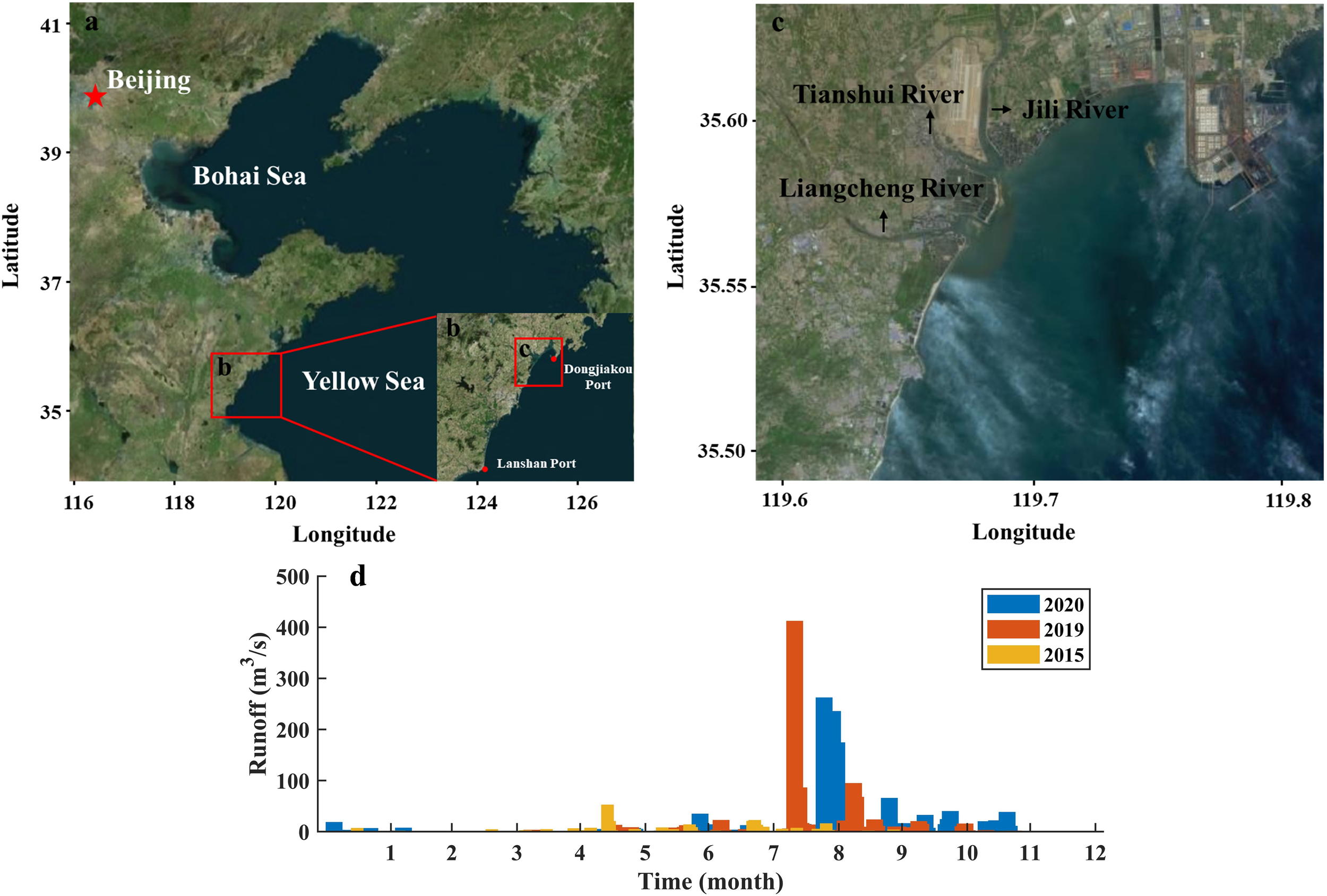
Figure 1. Geographic location of study area (a–c) and distribution of annual runoff of Liangcheng River in 2015, 2019 and 2020 (d).

The study area is dominated by an irregular semidiurnal tidal regime, with asymmetrical flood and ebb durations. Flood currents are generally stronger than the ebb currents, and surface currents exhibit the highest velocities in the vertical direction. The prevailing wave directions range from ESE to SSE, accounting for approximately 59.52%, among which SE-direction waves are the most frequent. The wave climate is primarily characterized by a mixture of wind waves and swell, with a maximum observed significant wave height of approximately 3.6 m. The frequency of waves with a height less than 0.7 meters is about 74%.

2.2 Numerical model

Delft3D is a multidimensional modeling software developed by Delft University of Technology. The software is well known for its flexible framework and excellent performance, particularly in simulating two-dimensional and three-dimensional hydrodynamics, waves, water quality, ecology, sediment transport, bed morphology, and the interactions among these processes. The Delft3D model system consists of seven major modules: FLOW (hydrodynamics), SEDIMENT (sediment transport), PART (particle tracking), WAQ (water quality), WAVE (waves), ECO (ecology), and MOR (morphology), all of which are open source (Deltares, 2014). To better represent complex terrains, Delft3D employs an orthogonal curvilinear coordinate system, which reduces simulation errors that may arise in curvilinear coastal and riverine boundaries (Dissanayake et al., 2012; Van der Wegen and Roelvink, 2012).

Delft3D has been widely applied to simulate hydrodynamic and sedimentary processes in various estuarine and coastal systems worldwide. In China, it has been successfully implemented in several large estuaries, such as the Changjiang (Yangtze) Estuary (Hu et al., 2009; Kuang et al., 2013), the Qiantang Estuary (Xie et al., 2013, 2017), and the Pearl River Estuary (Twigt et al., 2009), demonstrating its capability to reproduce complex wave-current interactions and estuarine circulation patterns.

2.2.1 Model description

Delft-Flow solves the shallow-water Navier-Stokes equations based on the hydrostatic pressure difference method. In the vertical momentum equation, vertical acceleration is ignored, and the hydrostatic pressure equation is obtained. In 3D simulation, the vertical velocity is calculated based on the continuity equation. In the horizontal direction, Delft-Flow uses orthogonal curve coordinates and supports two coordinate systems: Cartesian coordinate system (ξ, η) and spherical coordinate system (λ, ϕ). The conversion relationship between the two coordinate systems is as follows (Equation 1):

$\begin{array}{ll}\begin{array}{c}\xi =\lambda ,\eta =\varphi \\ \sqrt{G_{\xi \xi }}=R\text{ cos }\varphi ,\sqrt{G_{\eta \eta }}=R\end{array}& (1)\end{array}$

in which $\lambda$ is the longitude, $\phi$ is the latitude and R is the radius of the Earth (6378.137 km, WGS84), $\sqrt{G_{\xi \xi }}$ is the coordinate transformation coefficient in $\xi$ direction, $\sqrt{G_{\eta \eta }}$ is the coordinate transformation coefficient in $\eta$ direction.

Vertically, Delft-FLOW provides two different vertical grid systems: the σ coordinate system and the Cartesian Z coordinate system. This article uses the σ coordinate system. The vertical grid of the σ coordinate system is defined by two σ planes, namely the liquid free surface and the seabed. When activating the σ coordinate system, it is necessary to specify the number of vertical layers and the thickness ratio of each layer (the sum of all layer ratios is 100%). In this article, the vertical direction is divided into 5 layers, and the thickness percentages of each layer from the free surface to the seabed are 40, 27, 18, 10, and 5, respectively. The σ coordinate system is defined as (Equation 2):

$\begin{array}{ll}\sigma =\frac{z-\zeta }{d+\zeta }=\frac{z-\zeta }{H}& (2)\end{array}$

z is the vertical coordinate in physical space (Cartesian coordinate system); ζ is the elevation of the free surface above the reference plane (z = 0); d is the water depth below the reference plane; H is the total water depth (H = d + ζ) (Figure 2).

Figure 2

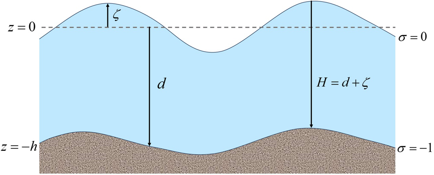
Figure 2. Parameter diagram (Deltares, 2014).

In the σ coordinate system, the governing equations of Delft-Flow are as follows:

Continuity equation:

$\begin{array}{ll}\frac{\partial \zeta }{\partial \text{t}}+\frac{1}{\sqrt{G_{\xi \xi }}\sqrt{G_{\eta \eta }}}\frac{\partial [(d+\zeta )u\sqrt{G_{\eta \eta }}]}{\partial \xi }+\frac{1}{\sqrt{G_{\xi \xi }}\sqrt{G_{\eta \eta }}}\frac{\partial [(d+\zeta )v\sqrt{G_{\xi \xi }}]}{\partial \eta }+\frac{\partial \omega }{\partial \sigma }=(d+\zeta )(q_{in}-q_{out})& (3)\end{array}$

ξ−directional momentum equation:

$\begin{array}{ll}\begin{array}{c}\frac{\partial u}{\partial t}+\frac{u}{\sqrt{G_{\xi \xi }}}\frac{\partial u}{\partial \xi }+\frac{v}{\sqrt{G_{\eta \eta }}}\frac{\partial u}{\partial \eta }+\frac{\omega }{d+\zeta }\frac{\partial u}{\partial \sigma }\\ -\frac{v^2}{\sqrt{G_{\xi \xi }}\sqrt{G_{\eta \eta }}}\frac{\partial \sqrt{G_{\eta \eta }}}{\partial \xi }+\frac{uv}{\sqrt{G_{\xi \xi }}\sqrt{G_{\eta \eta }}}\frac{\partial \sqrt{G_{\xi \xi }}}{\partial \eta }-fv\\ =-\frac{1}{{\rho }_0\sqrt{G_{\xi \xi }}}{P}_{\xi }+F_{\xi }+\frac{1}{{(d+\zeta )}^2}\frac{\partial }{\partial \sigma }({\nu }_v\frac{\partial u}{\partial \sigma })+M_{\xi }\end{array}& (4)\end{array}$

η−directional momentum equation:

$\begin{array}{ll}\begin{array}{c}\frac{\partial v}{\partial t}+\frac{u}{\sqrt{G_{\xi \xi }}}\frac{\partial v}{\partial \xi }+\frac{v}{\sqrt{G_{\eta \eta }}}\frac{\partial v}{\partial \eta }+\frac{\omega }{d+\zeta }\frac{\partial v}{\partial \sigma }\\ -\frac{u^2}{\sqrt{G_{\xi \xi }}\sqrt{G_{\eta \eta }}}\frac{\partial \sqrt{G_{\xi \xi }}}{\partial \eta }+\frac{uv}{\sqrt{G_{\xi \xi }}\sqrt{G_{\eta \eta }}}\frac{\partial \sqrt{G_{\eta \eta }}}{\partial \xi }+fu\\ =-\frac{1}{{\rho }_0\sqrt{G_{\eta \eta }}}{P}_{\eta }+F_{\eta }+\frac{1}{{(d+\zeta )}^2}\frac{\partial }{\partial \sigma }({\nu }_v\frac{\partial v}{\partial \sigma })+M_{\eta }\end{array}& (5)\end{array}$

The ω in Equations 3–5 is the vertical velocity relative to the σ plane, which can be interpreted as the velocity related to the motion of the upwelling or descending flow. The actual vertical velocity w is calculated based on the mass conservation equation (Equation 3) using the horizontal velocity, water depth, water level, and vertical velocity ω in the σ coordinate system (Equation 6):

$\begin{array}{ll}w=\omega +\frac{1}{\sqrt{G_{\xi \xi }}\sqrt{G_{\eta \eta }}}[u\sqrt{G_{\eta \eta }}(\sigma \frac{\partial H}{\partial \xi }+\frac{\partial \zeta }{\partial \xi })+v\sqrt{G_{\xi \xi }}(\sigma \frac{\partial H}{\partial \eta }+\frac{\partial \zeta }{\partial \eta })]+\left(\sigma \frac{\partial H}{\partial t}+\frac{\partial \zeta }{\partial t}\right)& (6)\end{array}$

in Equations 3–6, u, v, and ω represent the velocity components in the ξ-, η-, and σ-directions, respectively. q_in and q_out denote the source and sink terms representing the volume of fluid entering or leaving a unit volume of the medium per unit time. ρ₀ is the seawater density. P_ξ and P_η are the pressure gradient terms, while F_ξ and F_η represent the Reynolds stress terms induced by turbulence. M_ξ and M_η are the external momentum source/sink terms, which include external forces such as those induced by hydraulic structures, water withdrawal or discharge, and wave stresses. f is the Coriolis parameter, given by f = 2Ω sinϕ, where Ω is the angular velocity of Earth’s rotation. ν_v is the vertical eddy viscosity coefficient, calculated using Equation 7.

$\begin{array}{ll}{\nu }_v={\nu }_{mol}+\text{max }({\nu }_{3D},{\nu }_v^{back})& (7)\end{array}$

in which ν_mol is the molecular turbulent viscosity coefficient, ν_3D is the three-dimensional turbulent viscosity coefficient, and ${\nu }_v^{back}$ is the background turbulent viscosity coefficient.

Delft-FLOW solves the momentum conservation equations and the continuity equation using the ADI (Alternating Direction Implicit) method to obtain the hydrodynamic field at each time step. The time step Δt is generally determined by the CFL (Courant-Friedrichs-Lewy) number (Equation 8):

$\begin{array}{ll}CFL=2\text{Δ}t\sqrt{gh\left(\frac{1}{\text{Δ}{x}^2+\text{Δ}{y}^2}\right)}<4\sqrt{2}& (8)\end{array}$

in which, $\text{Δ}t$ is the time step, $g$ is the gravitational acceleration, and $\text{Δ}x$ ($\text{Δ}x=\sqrt{G_{\xi \xi }}$) and $\text{Δ}y$ ($\text{Δ}y=\sqrt{G_{\eta \eta }}$) are the minimum grid sizes in the $\xi$ and $\eta$ directions, respectively.

The Delft-WAVE module adopts the third-generation wave model SWAN to compute wave dynamics. It is capable of simulating random waves with a two-dimensional dynamic spectral density, using relative frequency σ_r and wave direction θ as independent variables. The wave action density is defined as the energy density divided by the relative frequency: N(σ_r, θ) = E(σ_r, θ)/σ_r. In SWAN, this spectrum may vary with both time and space. The dynamic spectral balance equation is expressed as (Equation 9):

$\begin{array}{ll}\frac{\partial }{\partial t}N+\frac{\partial }{\partial x}{c}_{x}N+\frac{\partial }{\partial y}{c}_{y}N+\frac{\partial }{\partial {\sigma }_r}{c}_{{\sigma }_r}N+\frac{\partial }{\partial \theta }{c}_{\theta }N=\frac{S}{{\sigma }_r}& (9)\end{array}$

The first term on the left-hand side of the equation represents the local rate of change of wave action density in time. The second and third terms describe the propagation in the geographic space x and y with velocities c_x and c_y, respectively. The fourth term accounts for changes in relative frequency due to variations in depth and currents (propagation in σ_r space with velocity c_σr). The fifth term represents refraction caused by depth and current variations (propagation in θ space with velocity c_θ). On the right-hand side of the equation, S denotes the source and sink terms of energy (Equation 10):

$\begin{array}{ll}S=S_{in}+S_{ds}+S_{nl}& (10)\end{array}$

in which, S_in represents the source term due to wind input; S_ds denotes the dissipation term caused by white capping, bottom friction, and depth-induced breaking; S_nl represents the nonlinear wave-wave interaction term.

The coupling between waves and currents can be implemented in either offline or online modes. In the offline coupling mode, the wave module calculates the relevant wave parameters at predefined time intervals for subsequent hydrodynamic computations. However, during this process, the hydrodynamics do not provide any feedback to the wave field. In contrast, the online coupling mode is more dynamic, enabling real-time information exchange between wave and hydrodynamic modules, thereby allowing mutual interaction in their computations.

2.2.2 Model setup and verification

In this study, the hydrodynamic module and wave module in Delft3D are used to perform wave-current coupled numerical simulations. The Delft3D-FLOW and WAVE modules are coupled in online mode, exchanging parameters every 360 seconds. Two sets of computational grids are employed. As shown in Figure 3a, the coarse grid covers the Bohai and Yellow Seas and is used to calculate regional hydrodynamic parameters, providing boundary inputs for a finer local grid (Figure 3b). The coarse grid is configured for two-dimensional hydrodynamic modeling, while the fine grid is used for three-dimensional simulations. To ensure computational efficiency while maintaining grid orthogonality and smoothness, local grid refinement is applied near the study area. The spatial resolution of the coarse grid ranges from 1.5 to 4.6 km, while the fine grid ranges from 40 to 800 m, with the highest resolution in the study area. Vertically, the fine grid adopts a five-layer σ-coordinate system, with increased resolution toward the seabed. In this study, the Manning coefficient is set as a spatially uniform constant because the computational domain coverage is relatively small with limited variation in seabed material. The constant value of 0.02 was adopted after calibration against measured data, ensuring good agreement between simulations and observations.

Figure 3

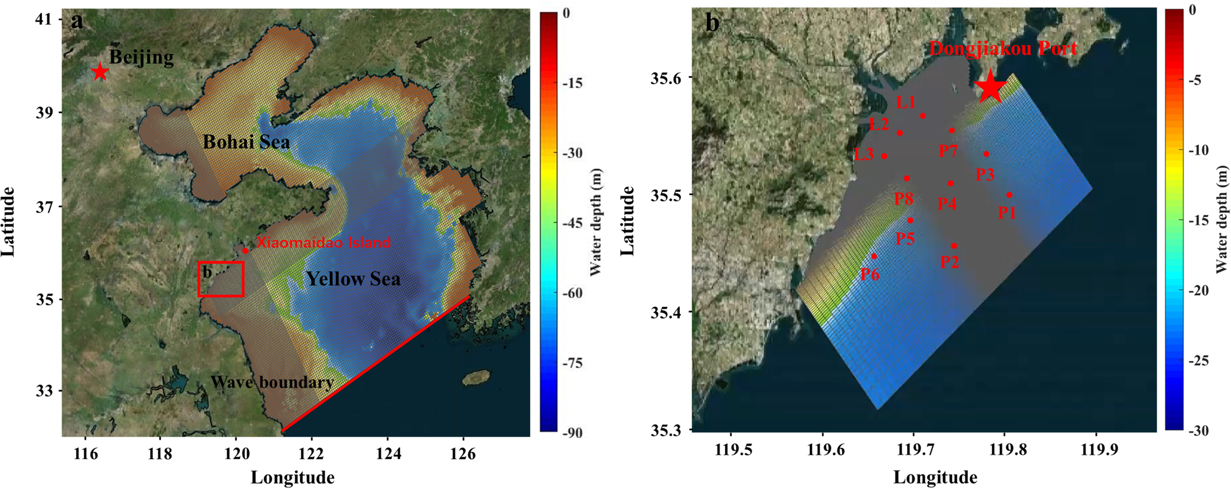
Figure 3. Numerical simulation calculation grid diagram. (a) Coarse grid and (b) finer grid.

The model bathymetry is based on 2018 digitized nautical chart data, and the simulation time step is set to 60 s. Open boundary conditions include wave, water level, and runoff. Wave boundary conditions for the fine grid are interpolated from the large-scale hydrodynamic simulation, which itself uses wave data from the ERA5 database (Hersbach et al., 2020). The water level boundary is extracted from the NAO.99b global tidal model (Matsumoto et al., 2000), incorporating eight primary constituents (K1, K2, M2, N2, O1, P1, Q1, and S2). There are three rivers entering the sea within the study area, with two on the north side converging before entering the sea. Daily runoff data are sourced from the Rizhao and Qingdao Hydrological Bureaus.

The model was calibrated and validated using measured data, including assessments of water level, current velocity and current direction. For the latter two parameters, validation was performed at the surface, mid-layer (0.6 H), and bottom layer. The spatial distribution of the validation sites is shown in Figure 3b. The location distribution of the verification sites is shown in Figure 3b, where P1 ∼ P8 was measured from August 1st to August 9th, 2015, and L1 ∼ L3 was measured from March 7th to March 10th, 2016. Model performance was quantitatively evaluated using the percent bias (PBIAS) (Moriasi et al., 2007), calculated as follows (Equation 11):

$\begin{array}{ll}PBIAS=100\times \left|\frac{{\displaystyle \sum }(M_i-S_i)}{{\displaystyle \sum }{M}_i}\right|& (11)\end{array}$

where M is the measured value and S is the simulated value. When the PBIAS values below 10 indicate excellent model performance; values between 10 and 20 are considered good; values between 20 and 40 are deemed fair; and values exceeding 40 suggest poor performance and the need for further model adjustment (Moriasi et al., 2007).

Supplementary Figure S1 presents the comparison between measured and simulated current velocity and direction at stations L1 to L3. The results demonstrate that the model can satisfactorily reproduce regional hydrodynamics. A good agreement is observed between measurements and simulations, with the best performance at the surface layer, followed by the middle layer (Supplementary Table S1).

The measurements at P1 ∼ P8 were conducted over 24-hour periods during spring, medium, and neap tides between August 1 and 9, 2015. As these data are temporally scattered, scatter plots were used to compare the measured and simulated values of current velocity and current direction (Supplementary Figures S2 and S3) to evaluate model accuracy. The results indicate good agreement between the simulated and measured currents and water levels (Supplementary Figure S4), with surface current velocities showing better consistency than bottom-layer values (Supplementary Table S2).

Wave data from the Xiaomaidao Island station (location shown in Figure 3a) were compared with the simulated results (Supplementary Figure S5). Supplementary Figures S5b, S5c include the significant wave height comparisons during the passage of Typhoon Matmo (2014) and Typhoon Lekima (2019), respectively. The measured and simulated wave heights show good agreement, with corresponding PBIAS and RMSE values confirming the model’s capability to accurately reproduce wave dynamics in the study area.

3 Results

Based on the three-dimensional hydrodynamic numerical model established in Section 2, this chapter simulated the hydrodynamic process of a typical wet year (2020) and studied the seasonal changes in hydrodynamics in the estuarine area. The control variable method was used to design different control numerical experimental groups, focusing on the analysis of the individual and combined effects of waves and runoff. Furthermore, the characteristic point and characteristic profile method was used to compare and explore the differences in hydrodynamic responses of the northern and southern estuaries under seasonal regulation.

In the wet year, summer runoff exhibits a substantial increase (Figure 1), leading to significant alterations in flow field distributions. Since seasonal variations in spring, autumn, and winter demonstrate relatively minor differences, this section focuses on comparing the differences in flow field characteristics between winter and summer under the wet year.

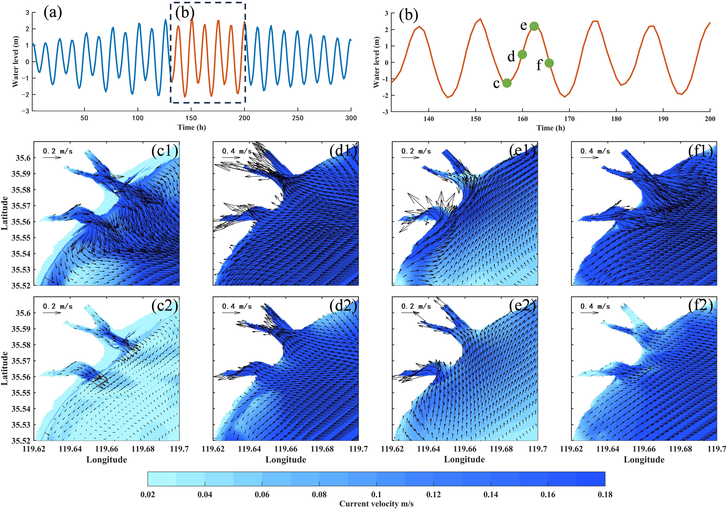
Figure 4 shows the flow field distribution during the winter neap tide. During slack ebb tide, the surface layer currents of the northern and southern estuaries are both toward the sea, with the current velocity of approximately 0.16 m/s. The surface current direction around the southern estuary is mainly southeast, and the distribution is relatively uniform. However, the flow field distribution around the northern estuary is more complex. There is a landward flow at the northern estuary, which conflicts with the seaward flow upstream, forming a low velocity zone, causing the velocity to decrease to 0.03 m/s. In the offshore area, affected by the estuarine jets, the current direction in the northeastern area is southeast-southwest, and the current direction in the southwest area is southeast-eastward. The bottom flow field distribution is similar to the surface in the nearshore area, but the velocity is greatly reduced.

Figure 4

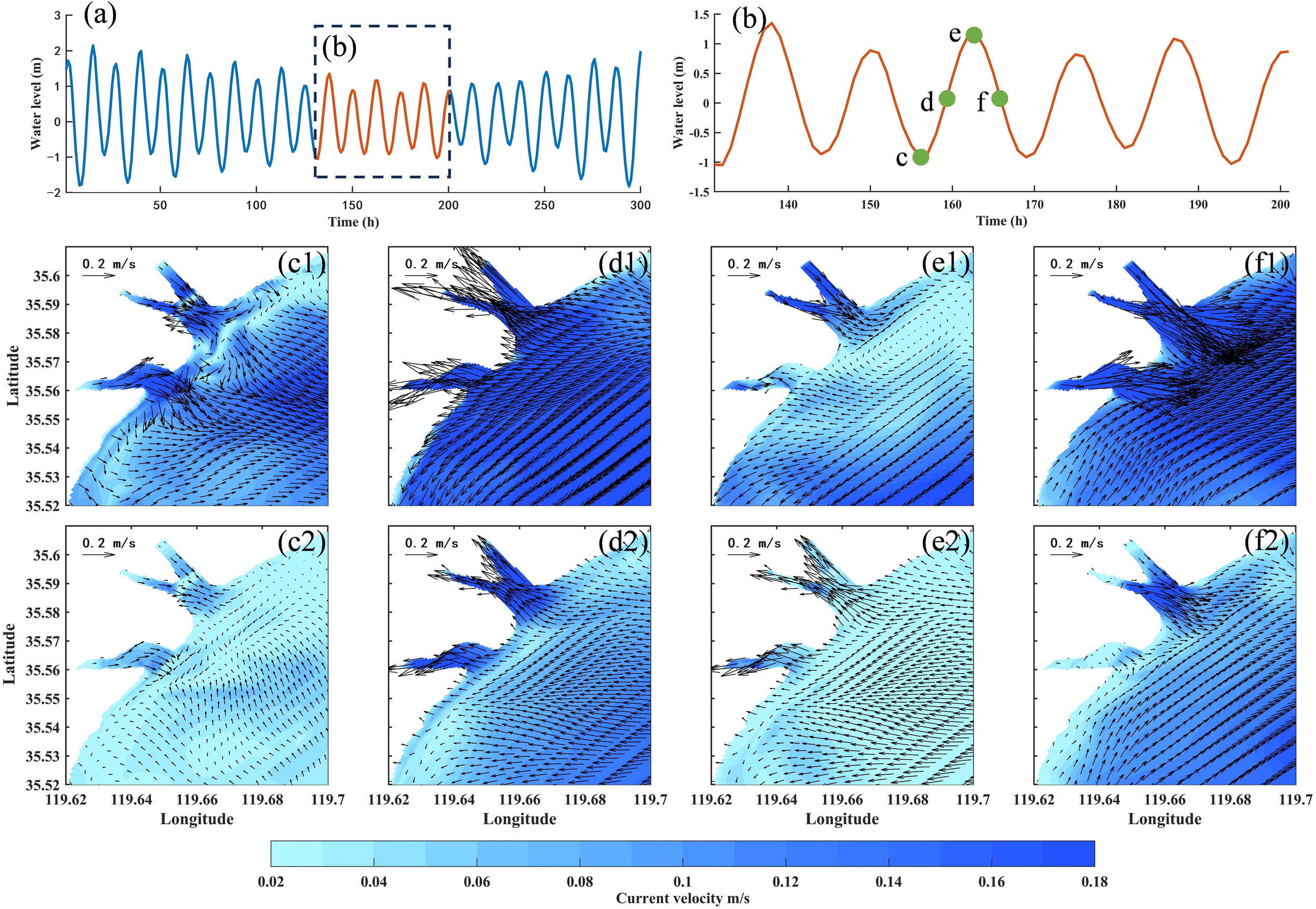
Figure 4. Distribution diagram of neap tide flow field in winter of wet year. (a, b) are water level diagrams; (c–f) respectively show the flow field distributions during slack at ebb tide, peak flood tide, slack at flood tide, and peak ebb tide; number 1 represents the surface flow field, number 2 represents the bottom flow field.

During peak flood tide, tides control the current velocity of the estuary, with both surface and bottom currents directed landward. Surface instantaneous velocities range 0.2 ∼ 0.6 m/s, while bottom velocities are significantly lower. During slack flood tide, the control of tides over the estuarine current is significantly weakened. Surface currents in the northern estuary reverse to seaward, forming a counterclockwise circulation with offshore flood currents near the estuarine area. The impact of runoff on the bottom layer is relatively weak, with upstream bottom current maintaining flood current direction. During peak ebb tide, the direction of ebb currents align with runoff, generating reinforced seaward currents at the surface with maximum instantaneous velocities reaching 0.7 m/s. The bottom flow field exhibits similar spatial patterns to the surface, but the current velocity is significantly smaller, with the greatest decrease at the estuary.

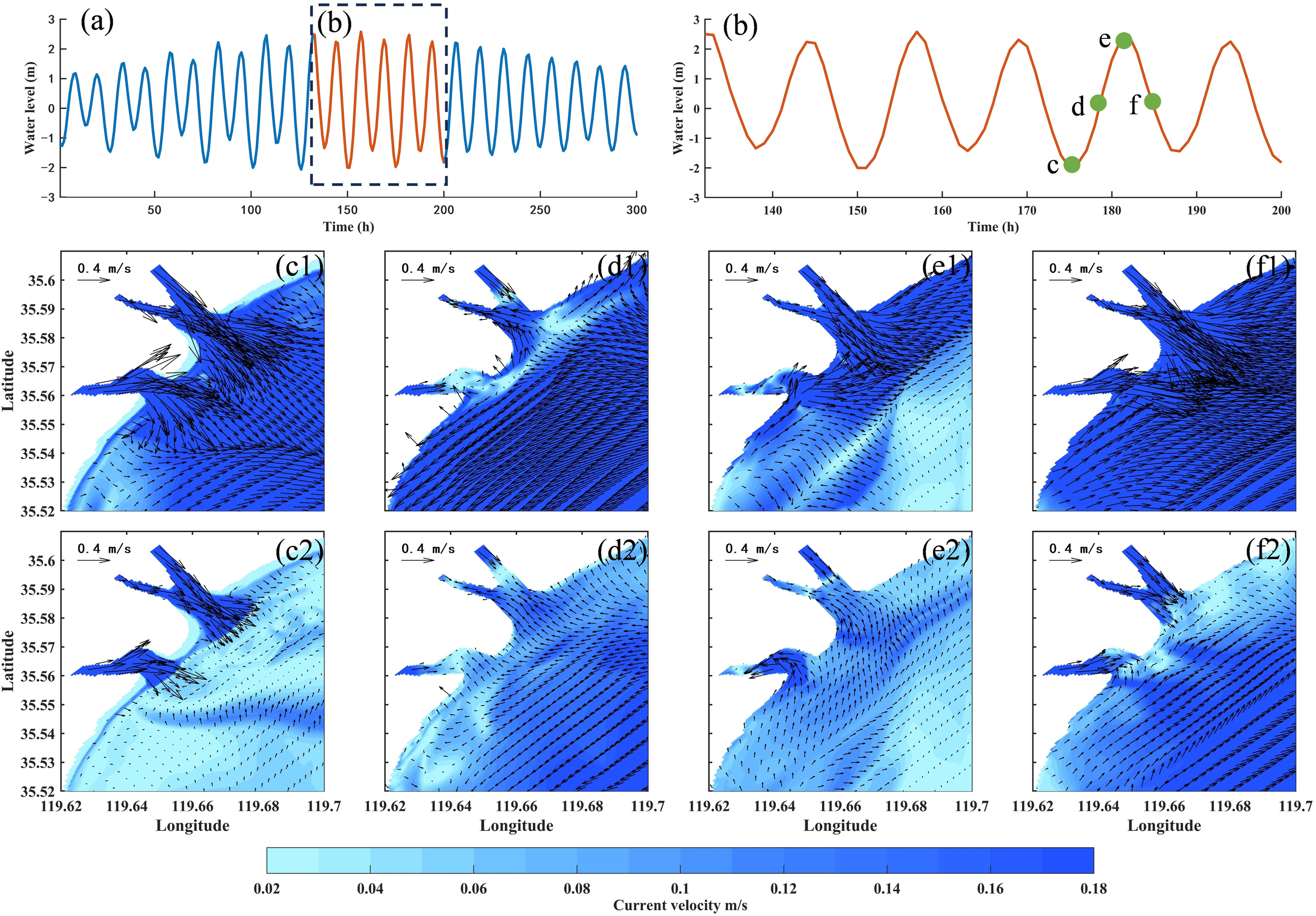
Figure 5 shows the flow field distribution during winter spring tide. Due to the significant tidal range of the spring tide, the momentum exchange is enhanced during the tidal cycle. Even during the slack ebb tide, the study area still maintains strong background current velocity (mainly southwestward offshore current), with significantly higher surface velocity than during the neap tide period. The bottom flow field shows spatial differentiation characteristics: the estuarine area is seaward, while other areas have complex flow patterns and weaker current velocity.

Figure 5

Figure 5. Distribution diagram of spring tide flow field in winter of wet year. (a, b) are water level diagrams; (c–f) respectively show the flow field distributions during slack at ebb tide, peak flood tide, slack at flood tide, and peak ebb tide; number 1 represents the surface flow field, number 2 represents the bottom flow field.

During peak flood tide, landward currents dominate both surface and bottom layers with velocities significantly exceeding neap tide period (surface: 0.4 ∼ 0.9 m/s; bottom: 0.06 ∼ 0.5 m/s). During slack flood tide, as the tidal forcing gradually weakens, runoff influence becomes predominant in the northern upstream estuary, driving seaward currents. This seaward currents converge with landward flood currents near the estuary area, forming a low-velocity zone. Both surface and bottom current velocities decrease significantly compared to peak flood tide, shifting northward as the currents transition toward ebb tide. Notably, the surface flow field along the southwest nearshore completes this flood-to-ebb transition earlier than the surrounding waters. During peak ebb tide, the flow field distribution during spring tide resembles that of neap tide, but intensified tidal forcing increases current velocity to 2 ∼ 3 times that of neap tide.

During summer spring tide (Figure 6), there is a significant difference in flow field distribution compared to winter due to strong runoff. During slack ebb tide, the water level drops and nearshore current velocity decreases, but the velocity is still higher than during winter spring slack ebb tide. Enhanced by strong runoff input, the seaward flow intensifies significantly throughout the study area, with the most obvious changes occurring in estuarine and river channel areas, which is about 2 ∼ 5 times than winter spring tide values.

Figure 6

Figure 6. Distribution diagram of spring tide flow field in summer of wet year. (a, b) are water level diagrams; (c–f) respectively show the flow field distributions during slack at ebb tide, peak flood tide, slack at flood tide, and peak ebb tide; number 1 represents the surface flow field, number 2 represents the bottom flow field.

During peak flood tide, the enhanced tidal forcing compresses the runoff control range to the upstream of the estuary. The runoff-dominated seaward currents and tide-dominated landward currents counteract within the river channel, causing instantaneous velocity to drop from 0.36 m/s to 0.03 m/s. During slack flood tide, as flood tidal forcing diminishes, the runoff-dominated zone extends seaward to approximately the 7 m isobath, driving the surface flow field to shift southeastward. Beyond the 7 m isobath, runoff influence on surface flow field diminishes while northwestward tidal currents dominate, albeit with generally reduced velocities due to energy dissipation. This surface flow field characteristic synchronously affects the bottom hydrodynamic structure: the bottom current direction on the land side of the 7 m isobath is northeastward, and turns to the southeast on the seaward side, forming a distinct hydrodynamic boundary. During peak ebb tide, strong tidal forcing combines with co-directional strong runoff, causing the instantaneous seaward current velocity reaches the maximum. The maximum surface velocity can reach 1.2 m/s, and the bottom velocity is mainly distributed between 0.2 ∼ 0.4 m/s.

The current velocity exhibits significant spatial variability in the study area. To investigate the spatial heterogeneity of the flow field, three characteristic points were selected—the northern estuary (characteristic point 1), southern estuary (characteristic point 2), and offshore region (characteristic point 3) (Figure 7a)—for a comparative analysis of surface and bottom velocity distributions under different tidal periods. During the winter neap tide (Figure 7b), the velocity at the characteristic point 1 is the largest, followed by the characteristic point 2 and the velocity at the characteristic point 3 is the smallest. The velocities at the characteristic points exhibit tidal-phase-dependent variations, with a distinct double-peak pattern emerging during ebb tides in the estuarine area, indicative of nonlinear hydrodynamic interactions between tidal forcing and wave deformation. The bottom velocity fluctuation is synchronized with the surface layer, but its value and variation are smaller than the surface layer, suggesting enhanced energy dissipation near the bed.

Figure 7

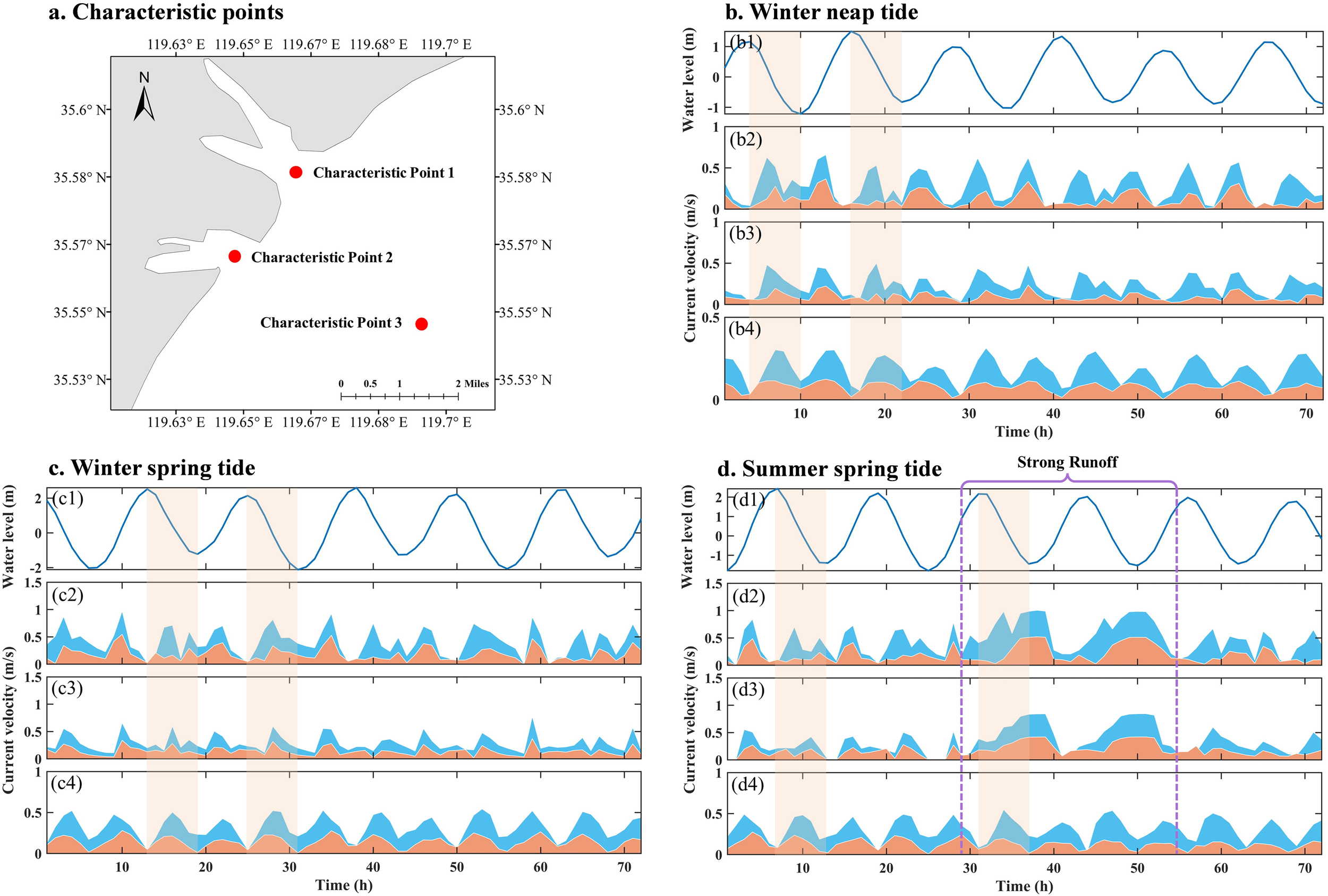
Figure 7. (a) Location of characteristic points. (b) Current velocity distribution of characteristic points during winter neap tide: (b1) water level, (b2) velocity at point 1, (b3) velocity at point 2 and (b4) velocity at point 3. The blue fill indicates the surface velocity, while the orange fill indicates the bottom velocity. The orange shading corresponds to the part of ebb-tide process. (c) Current velocity distribution of characteristic points during winter spring tide. (d) Current velocity distribution of characteristic points during summer spring tide. The purple dashed line represents the strong runoff process.

In contrast to the estuarine area dominated by complex topography and runoff-tide interactions, the offshore area exhibits more regular tidal-period velocity variations without the double-peak observed in the estuary. The persistent seaward runoff promotes the development of ebb-dominated current in the offshore area, with the most significant flood-ebb asymmetry occurring in surface layer velocity (the ebb current velocity increases by about 10% ∼ 30% compared to the flood current). During winter spring tide (Figure 7c), the velocity at each characteristic point increases by a factor of 1.2 ∼ 1.8 relative to winter neap tide. Despite the increase in velocity, its spatial distribution pattern (northern estuary > southern estuary > offshore) and temporal evolution characteristics (such as phase relationships, vertical structure) remain highly similar to those of neap tide.

During the summer spring tide (Figure 7d), the current velocity distribution patterns under weak runoff are similar to those of the winter spring tide. When subjected to strong runoff forcing (29th hour in Figure 7d), the estuarine characteristic points demonstrate rapid velocity amplification, with the most pronounced enhancement occurring during ebb tides. Peak velocities at slack ebb tide reach 0.98 m/s and 0.85 m/s at the northern and southern estuarine characteristic points respectively, which is about twice that before the strong runoff. Throughout the strong runoff period, the velocity in the estuary area is maintained in the high value range except for a temporary attenuation during the flood tides. When the strong runoff effect ends (55th hour in Figure 7d), the flow velocity quickly returns to the background state. In contrast, the flow field in offshore (characteristic point 3) is relatively stable throughout the summer spring tide, indicating that the impact of strong runoff is mainly confined to the estuarine area.

Figure 8a illustrates the boxplots of surface current velocities at each characteristic point. The results demonstrate that the spatiotemporal variability of surface currents is governed by the combined influences of tidal dynamics, runoff, and topographic conditions, exhibiting pronounced seasonal variations and spatial heterogeneity. On the temporal scale, current velocity exhibits obvious tidal periodicity. During the winter neap tide, hydrodynamic conditions are weakest, resulting in the smallest velocity fluctuation ranges and the lowest median velocities among the three periods. During the winter and summer spring tides, the tidal range significantly increases and the current velocity changes more dramatically. The median velocity of the summer spring tide is the highest, followed by the winter spring tide. This is mainly attributed to differences in tidal range and seasonal variations in runoff intensity. Further comparison reveals that the velocity during winter neap is lower and changes steadily, while during the summer spring tide, strong tidal forces combined with runoff during the wet season result in significantly higher velocities and more severe fluctuations.

Figure 8

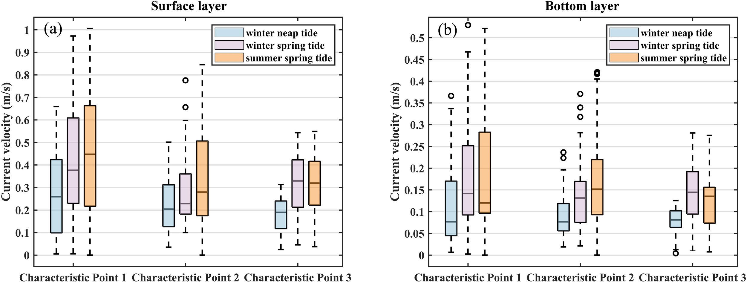
Figure 8. Velocity box plot of each point. (a) surface layer, (b) bottom layer. Blue represents winter neap tide, pink represents winter spring tide, and orange represents summer neap tide (time period: 72 hours).

Spatially, the near-estuary and offshore regions display distinct current velocity distributions. The interquartile range (IQR) of characteristic point 1 is the largest among all points across different periods, indicating the strongest variability in its time series of current velocities. Additionally, the velocity distributions at the near-estuary points (characteristic points 1 and 2) are right-skewed, whereas the offshore point (point 3) is less affected by runoff and topography, showing a more symmetric distribution with greater spatial uniformity. Notably, both the mean velocity and fluctuation amplitude at characteristic point 1 are the highest among all characteristic points, which is likely due to hydrodynamic intensification caused by the interaction between runoff and tides in the estuary area.

Figure 8b presents the boxplots of bottom current velocities at each characteristic point. The magnitudes of bottom current velocities are significantly smaller than those of the surface (Figure 8a), and the interquartile ranges (IQRs) are also smaller, indicating weaker variability in bottom currents. Moreover, the occurrence of outliers is more frequent in bottom current velocities than in surface, with this phenomenon being especially prominent at the southern estuarine point (characteristic point 2). The distribution patterns of bottom currents are predominantly governed by the combined influences of seabed topography and sediment. Complex terrain changes can significantly alter the structure of the underlying flow field, leading to abnormal fluctuations and the emergence of outliers. In particular, at characteristic point 2 within the southern estuary, the steep frontal slope and complex shoreline shape contribute to the most pronounced occurrence of bottom velocity outliers. These anomalous currents contrast sharply with the relatively stable distribution observed in surface currents, highlighting the distinctive hydrodynamic response characteristics of the near-bed boundary layer.

Residual currents refer to the components of ocean currents after removing the periodic astronomical tidal constituents, including wind-induced currents, density currents, tidal induced residual currents, etc. As the net transport flow field after filtering out periodic motions, residual currents can more clearly reveal the net material transport trends within the study area. The calculation formula usually involves averaging or integrating current velocity data over one or more cycles. The formula used in this section to calculate residual current is as follows (Equation 12):

$\begin{array}{ll}\overrightarrow{V_r}=\frac{1}{T}{\displaystyle {\int }_0^T\overrightarrow{V_i}dt}& (12)\end{array}$

where T denotes the duration used for the residual current calculation, typically covering multiple tidal cycles (three tidal cycles in this study), and $\overrightarrow{V_i}$ represents the velocity vector at the i time step.

Figure 9 shows the spatial distributions of seasonal mean residual currents in the surface layer, bottom layer, and vertically averaged during winter and summer of the wet year. The residual current field in the study area exhibits significant three-dimensional spatial heterogeneity, with the surface residual currents being the strongest. In winter, the maximum surface residual current reaches 0.15 m/s, occurring in the northern estuary and indicating seaward transport. Moving seaward, the influence of runoff gradually weakens, and the residual currents at the northern estuary decrease markedly to approximately 0.02 m/s. In contrast, the residual current distribution in the southern estuary is more complex due to the larger channel curvature and the comparable widths of the inlet and river channel. The residual currents at the southern estuary remain around 0.04 m/s, while a pronounced high-value zone (0.1 m/s) is observed around the bend, which may result from flow convergence induced by the locally protruding shoreline. Along the coastal regions, the northern coast exhibits a stable northeastward alongshore currents, whereas the southern coast is dominated by a southwestward alongshore currents, accompanied by a nearshore northeastward return currents, forming a small-scale circulation system. The offshore area generally shows a seaward transport pattern, with a small high-value residual current zone observed in the southeastern sea area.

Figure 9

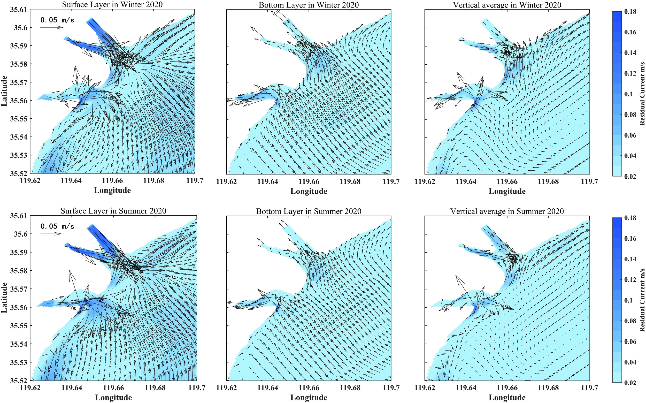
Figure 9. Distribution diagram of seasonal average residual current in wet year. The first row shows the distribution of surface, bottom and vertical average residual current in winter; the second row shows the distribution of surface, bottom and vertical average residual current in summer.

Figure 9 illustrates that in the nearshore area, the bottom residual currents are mostly northeastward alongshore currents, whereas around the estuary, current velocities increase due to the topographic constriction effect, with maximum bottom residual current reaching approximately 0.06 m/s. Compared to the surface residual currents, the bottom residual currents exhibit markedly reduced intensity and has an opposite direction. This vertical shear characteristic constitutes a typical estuarine circulation system. The formation mechanism of this circulation is mainly attributed to the baroclinic effect driven by salinity gradients. When low-salinity freshwater interacts with high-salinity seawater, pronounced density stratification develops. The density of surface freshwater is relatively low, floating on the surface and spreading seaward, while the high-density seawater at the bottom is driven landward under the influence of baroclinic pressure gradient forces, thereby forming a vertical circulation pattern (Hughes and Rattray, 1980; Dyer and Ramamoorthy, 1969). This gravitational circulation is a typical dynamic characteristic of estuarine areas, exerting crucial regulatory effects on material transport and energy balance.

In the deep-water region, the vertically averaged residual currents are relatively weak, with a localized clockwise circulation observed in the southeastern area. The estuarine area exhibits a complex flow structure: within the northern estuarine channel, the residual currents are directed seaward, but shifts landward just outside the estuary; in contrast, the residual currents within the southern estuarine channel are landward, forming a radial residual current distribution at the protruding shoreline. Compared to the surface and bottom residual currents, the vertically averaged residual current field displays a more uniform spatial distribution, reflecting the integral effect of vertical water column motion, which effectively smooths out local hydrodynamic variability. It is worth noting that although summer runoff is characterized by pronounced intermittent high-intensity transport, this short-term process becomes averaged out over the seasonal scale, resulting in a residual current pattern similar to that in winter.

4 Discussions

The results indicate that the hydrodynamic characteristics of the study area are significantly influenced by runoff and waves. Accordingly, this section presents a series of numerical experiments to systematically investigate the mechanisms through which wave-runoff interactions affect estuarine hydrodynamics.

4.1 Impact of wave

Wave-current interaction is a complex and dynamically significant process in marine dynamic systems (Mellor, 2003), with wave effects on currents realized through multiple mechanisms (Zhang et al., 2022). As waves propagate, periodic stress variations are generated on the sea surface, which induce water motion in the same direction as the waves (Yu et al., 2017). Additionally, wave-induced turbulence significantly enhances vertical exchange, thereby modifying the vertical structure of the flow field (Olabarrieta et al., 2010). Waves can also affect the strength and direction of currents by altering the dynamic characteristics of the bottom boundary layer, including the bottom friction coefficient and the shape of the velocity profile (Wolf and Prandle, 1999). These interaction effects exhibit significant differences under different water depths (Olabarrieta et al., 2011). A series of controlled numerical experiments (Supplementary Table S3) were designed to investigate the modulation effect of waves on the residual current field.

Figure 10a illustrates the seasonal average distribution of wave-induced residual currents during a wet year. In winter, the high-value zones of surface wave-induced residual currents are primarily located near the coast, predominantly exhibiting seaward rip currents. Scatter points with velocities exceeding 0.01 m/s are mainly distributed in areas with water depths less than 7 m (Figure 10b1). Within the estuarine channels, the residual currents display disorganized patterns, with mean velocities around 0.003 m/s. This spatial heterogeneity primarily results from the unique topographical conditions of the estuarine area: complex shoreline and shallow water conditions induce wave reflection and diffraction, interacting with incident waves to form complex wave fields. Moreover, lateral constraints imposed by river channel boundaries also influence the distribution of wave-induced residual currents at the estuary. Furthermore, both estuarine areas exhibit high-value zones of surface residual currents extending seaward, which are likely driven by seaward runoff (discussed further below). Offshore areas exhibit surface wave-induced residual currents of 0.002-0.005 m/s, generally directed seaward.

Figure 10

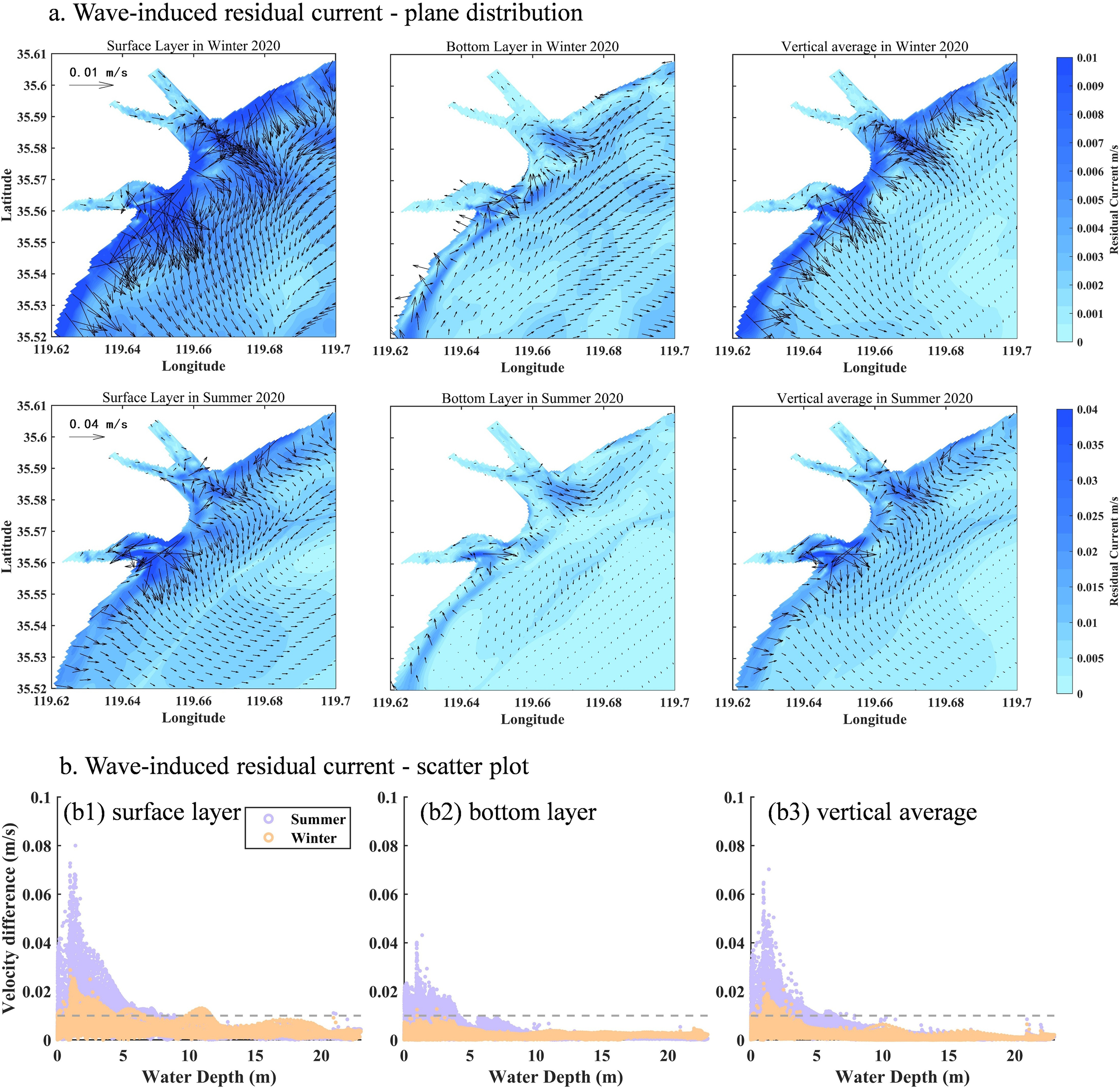
Figure 10. (a) The difference diagram of seasonal average wave-induced residual flow in wet year. The first row shows the difference distribution of surface, bottom and vertical average residual flow in winter; the second row shows the difference distribution of surface, bottom and vertical average residual flow in summer. (b) Scatter plot of wave-induced residual current and water depth in the study area. Purple scatter plots are summer, and orange scatter plots are winter.

As the vertical water depth increases, the intensity of wave-induced residual currents in the bottom layer significantly decreases due to energy dissipation during the momentum transfer process. Over 90% of bottom-layer velocities fall below 0.005 m/s (Figure 10b2). The impact of waves on residual currents exhibits spatial differences: the steep slope and complex shoreline along the southwest coast induce more intense and localized wave breaking, resulting in a greater influence of waves on the bottom residual currents compared to the northeast coast. In other regions, bottom wave-induced residual currents generally remain below 0.003 m/s. The vertically averaged wave-induced residual current field is directed seaward, with intensity decaying from nearshore to offshore. This distribution pattern reflects the significant enhancement of wave dynamics in the nearshore region and its rapid attenuation with increasing water depth.

In summer, high-value zones of surface wave-induced residual currents are also primarily distributed in estuarine and nearshore regions, dominated by offshore transport, with most surface velocities exceeding 0.02 m/s. Compared to winter, the nearshore wave-induced residual currents in summer are significantly enhanced, and areas with velocities greater than 0.01 m/s extend to the 8.5 m isobath (Figure 10b1). Due to topographic effects, stronger residual currents are observed near the southern estuary compared to the north. Bottom-layer patterns resemble those in winter but exhibit overall lower velocities. Notably, velocity discontinuities are observed in both surface and bottom layers near the 6 ∼ 7 m isobath, likely associated with wave breaking. The vertically averaged residual currents increase from offshore to nearshore, with high-velocity zones mainly concentrated within the 1 ∼ 3 m water depth range (Figure 10b3), similar to the pattern in winter.

When runoff is excluded (Figure 11a), surface wave-induced residual currents near the coast remain offshore-directed. However, the original high-value zones extending seaward at the northern and southern estuaries disappear, confirming that these zones are primarily formed by runoff. Surface wave-induced residual currents in the study area generally weaken, and the proportion of velocity exceeding 0.01 m/s drops markedly (Figure 11b1). The impact of runoff is particularly evident in the offshore area, where it enhances surface wave-induced residual currents and induces southward shifts. Furthermore, the inclusion of runoff also reverses the current direction in the southwestern offshore area—from southeastward to northeastward—indicating that runoff modulates both surface and bottom flow fields. Under no-runoff cases, vertically averaged wave-induced residual currents in the southwestern area exhibit broader weakening, while changes nearshore are limited, suggesting that winter runoff primarily affects the offshore area with only minor nearshore influence.

Figure 11

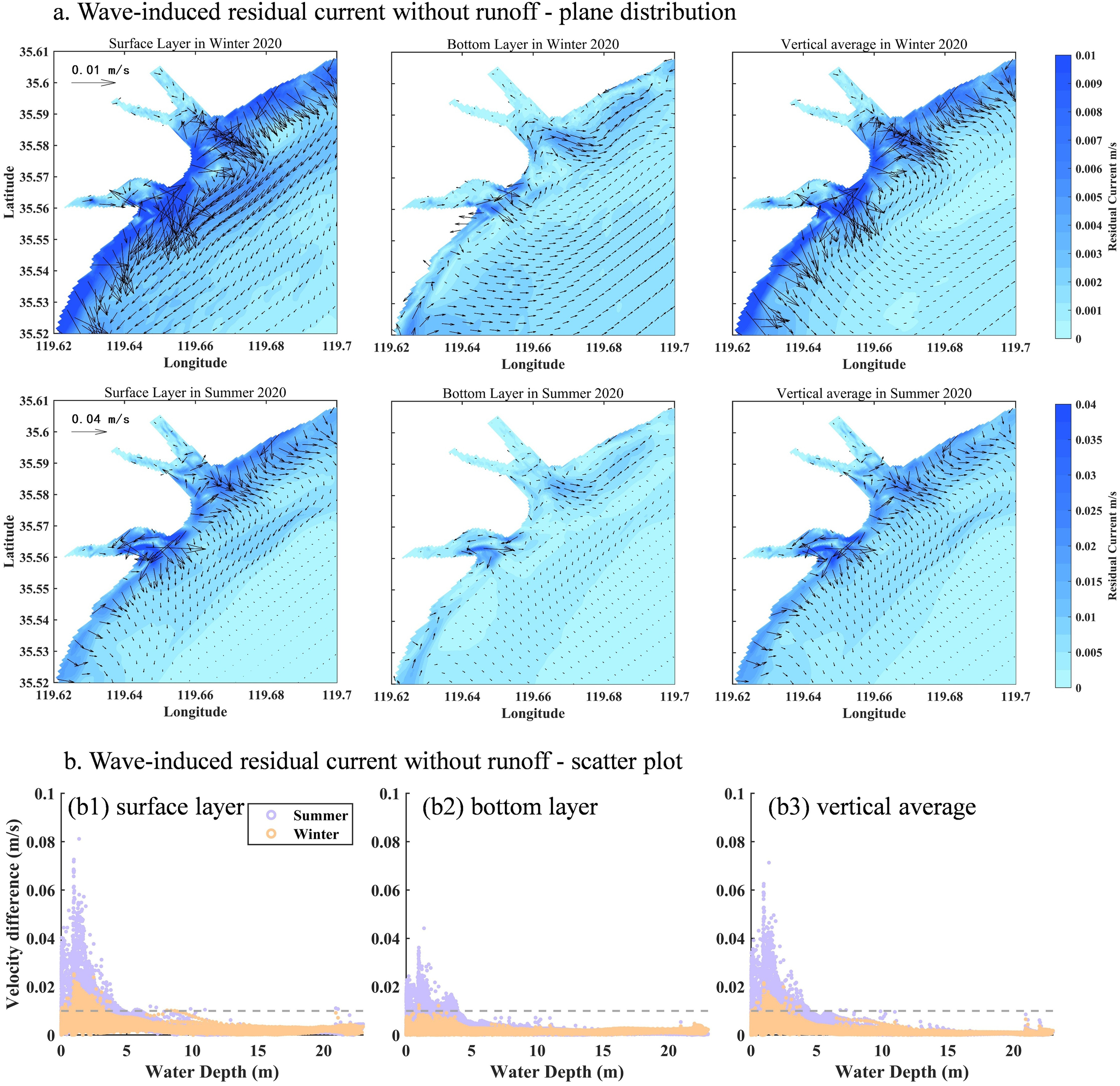
Figure 11. (a) The difference diagram of seasonal average wave-induced residual flow in wet year without runoff. The first row shows the difference distribution of surface, bottom and vertical average residual flow in winter; the second row shows the difference distribution of surface, bottom and vertical average residual flow in summer. (b) Scatter plot of wave-induced residual current without runoff and water depth in the study area. Purple scatter plots are summer, and orange scatter plots are winter.

During high-runoff conditions in summer, the removal of runoff leads to a substantial reduction in wave-induced residual currents across the study area. The surface current direction remains seaward, but the high-value zones near both estuaries contract, with a more pronounced decrease around the southern estuary. The most significant reductions occur within the 0 ∼ 5 m depth range, where the number of data points with velocities between 0.01 and 0.04 m/s drops sharply (Figure 11b1). In addition, the surface wave-induced residual current beyond the 6m isobath decreases from 0.015 m/s to 0.002 m/s, and the current direction shifts from southward to southwestward, highlighting the essential role of runoff in sustaining offshore-directed residual currents. Compared to the surface layer, the response of bottom wave-induced residual currents to runoff changes is relatively weak, with reductions mainly concentrated in the nearshore areas and smaller velocity attenuation than that at the surface.

In summary, the impact of waves on the residual currents in the study area is primarily concentrated in the nearshore areas and gradually weakens offshore. In the wet year, the intensity of wave-induced residual currents in summer is approximately four times that in winter, which is directly attributed to stronger wave forcing during the summer. Moreover, a velocity discontinuity emerges near the 6 m isobath due to wave breaking. Comparative experimental results indicate that the addition of runoff significantly enhances wave-induced residual current. In the absence of runoff, the intensity of wave-induced residual currents decreases markedly throughout the entire study area.

4.2 Impact of runoff

Runoff, as a key driving factor of the estuarine dynamic system, has a significant impact on the distribution of residual currents (Wang et al., 2008; Liu, 2011). The input of runoff breaks the original hydrodynamic equilibrium and enhances the complexity of the flow field (Simpson et al., 1993; Gao et al., 2009; Moon et al., 2010). Furthermore, the density gradient formed by freshwater input also significantly affects the vertical structure and stability of the flow field (Wu and Zhu, 2010; Palma and Matano, 2012). A series of numerical experiments was conducted to quantitatively assess the regulatory effect of runoff on the flow field (Supplementary Table S4). Given the relatively low runoff in winter during the wet year, the analysis in this section primarily focuses on the summer period.

In the case with runoff input solely from the northern estuary, the surface seaward residual currents are significantly intensified within the channel and along the jet axis, with the strongest enhancement within the channel (Figure 12, DE condition). Moving outward from the estuary, the intensity of the residual current gradually decreases due to channel expansion, accompanied by lateral dispersion toward both banks. Notably, a high-value zone of surface residual current difference appears near the southern estuary, which is closely associated with flow convergence and reflection effects induced by steep slopes and abrupt shoreline transitions. At the bottom layer, baroclinic forcing drives a compensating landward flow, with the high-value zone distribution closely mirroring that of the surface layer.

Figure 12

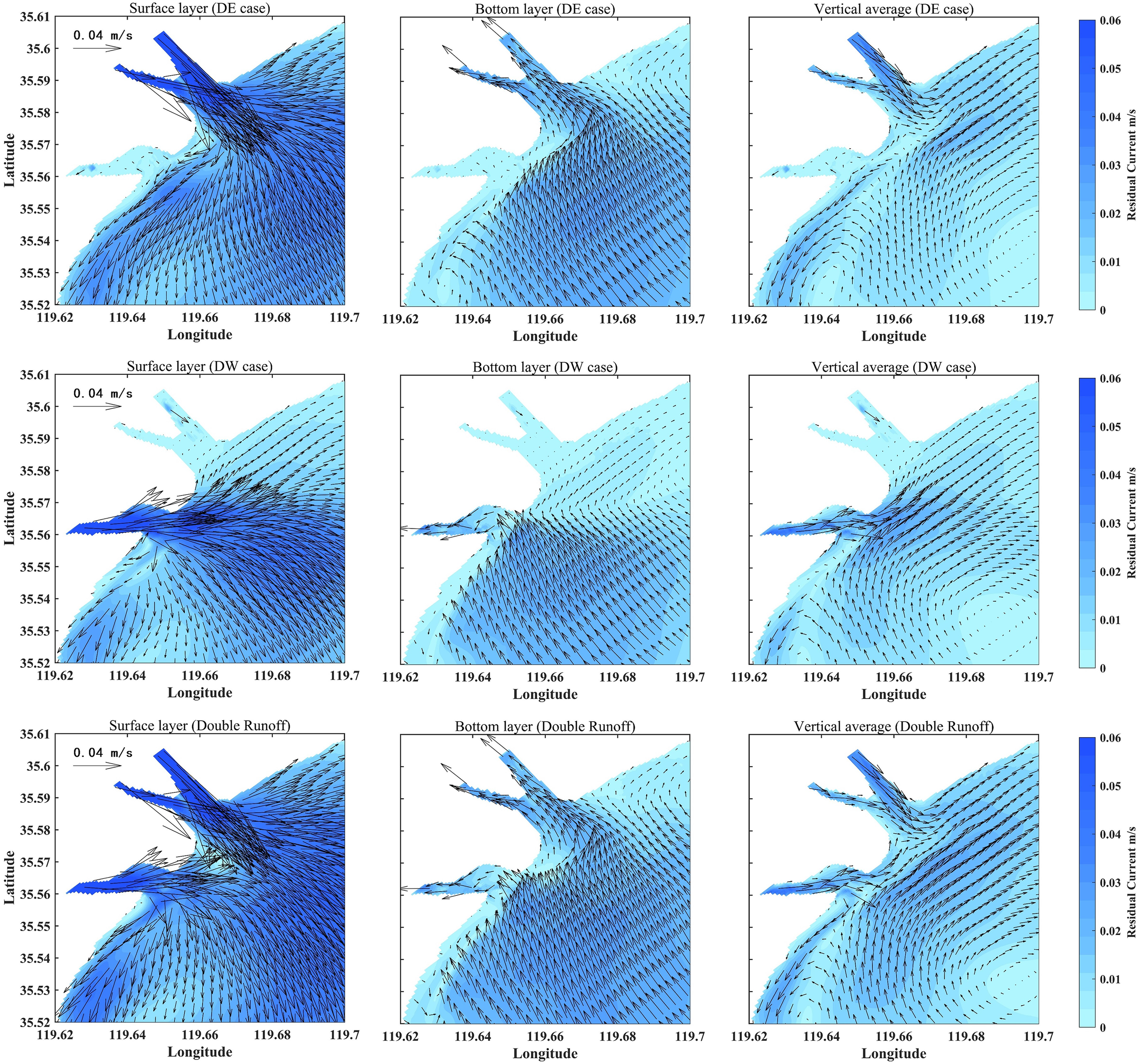
Figure 12. Distribution diagram of summer residual flow difference of different runoff experimental groups in wet year. The first line is the difference distribution between experimental group D and experimental group B; the second line is the difference distribution between experimental group E and experimental group B; the third line is the difference distribution between the baseline experiment and experimental group B.

When runoff is introduced exclusively from the southern estuary, the zone of maximum enhancement in residual currents remains centered along the channel and jet axis (Figure 12, DW case). However, its hydrodynamic characteristics are significantly different from the DE case. Due to the small angle between the jet axis and the shoreline, along with the narrow channel and irregular coastline, the generated alongshore currents are weak. The impact of the DW case on the alongshore residual currents on both sides of the estuary is substantially weaker than that of the DE case, especially in the northeastern area. In terms of vertical structure, runoff induces a landward compensation flow in the bottom layer, with high-value zones primarily located in the southwestern area, corresponding spatially to the surface layer. Vertically averaged residual currents show a clear seaward transport pattern in the southern estuary, although the velocity is high only near the estuary, with generally low velocities elsewhere. This spatial pattern highlights the critical role of local topographic constraints in shaping the runoff-driven hydrodynamics in the southern estuary.

When runoff is applied at both estuaries, the enhancement of residual currents within the channels reaches its maximum (Figure 12, DD condition). Compared to the single-runoff cases, residual currents in the northern offshore area are significantly stronger under the double-runoff case, while the enhancement near the southern estuary is comparatively weaker. This spatial differentiation primarily results from the differing flow characteristics and interactions between the two runoff sources. The northern runoff predominantly flows southeastward, while the southern runoff—modulated by the orientation of the estuary—intensifies the eastward component of residual currents and gradually deflects southward during offshore expansion, eventually converging with the northern runoff in the offshore region. Meanwhile, the diminished enhancement of residual currents near the southern estuary can be attributed to the mutual offset between the southwestward alongshore currents generated by the northern estuary and the northeastward residual currents from the southern estuary.

In summary, the input of runoff significantly enhances the surface residual current field in the study area, mainly manifested as the intensification of alongshore and offshore currents. Due to its wide estuarine mouth and gently sloping shoreline, the northern estuary exerts a broader influence range. In contrast, the southern estuary, constrained by the orientation of the mouth and the complex shoreline, produces a more confined offshore jet, resulting in a weaker impact on alongshore residual currents compared to the northern runoff. Under the double-runoff case, the residual currents around the northern estuary are significantly enhanced, while those around the southern estuary are clearly suppressed.

We selected the period of sustained strong runoff in summer and conducted a temporal analysis of the transverse and longitudinal components of the runoff-induced current at three characteristic points (Figure 13). Due to the highly consistent current distribution of the northern estuary under both the double-runoff and DE cases, characteristic point 1 only compares the current results of the double-runoff and DW cases (Figure 13a). Likewise, for characteristic point 2 in the southern estuary, the analysis compares only the double-runoff and DE cases (Figure 13b). The results indicate that in the absence of runoff, the velocities at the characteristic points approach zero. The addition of runoff significantly enhances the seaward and northeastward components of velocity at the estuaries, indicating that runoff input intensifies both offshore and alongshore currents. Specifically, the northern estuary runoff enhances the offshore current at characteristic point 1 (with a maximum increase of 1.3 m/s), while the southern estuary runoff primarily strengthens the northeastward alongshore current at characteristic point 2 (with a maximum increase of about 0.8 m/s). At characteristic point 3, the current distributions of the double-runoff and DE cases largely overlap, so only the results for the double-runoff and DW cases are plotted (Figure 13c). This suggests that the northern estuary runoff predominantly governs the offshore current field, primarily by enhancing the seaward component while weakening the northeastward component.

Figure 13

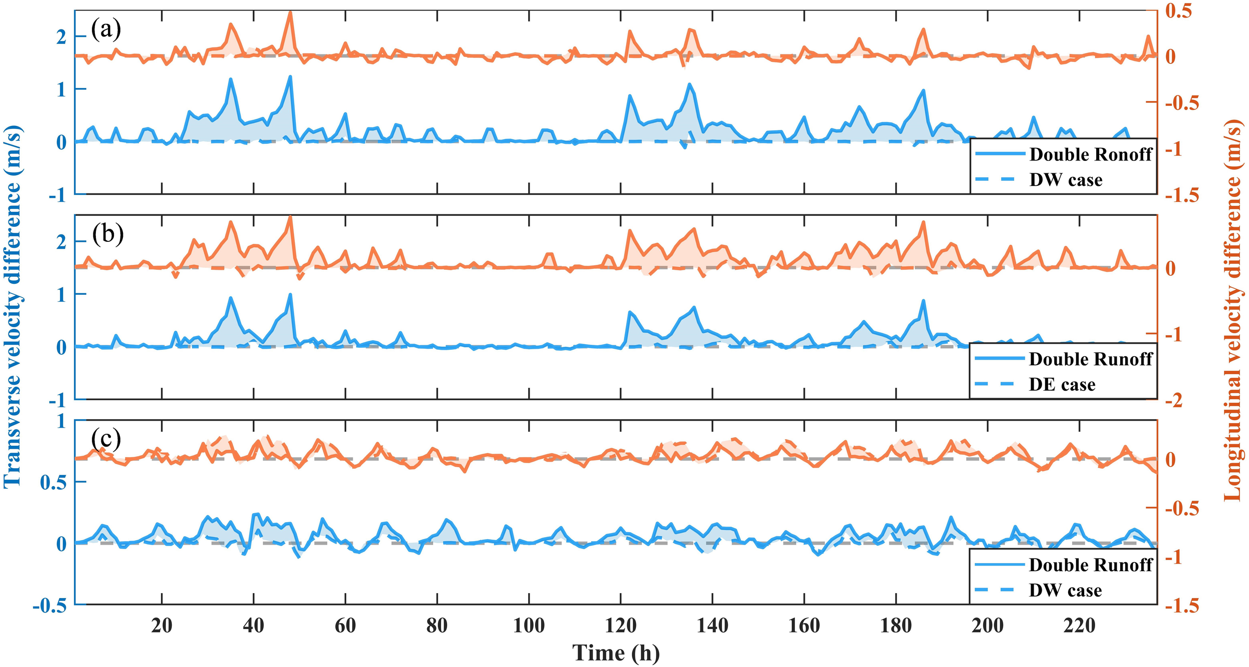
Figure 13. Time series distribution of residual flow at characteristic points. (a) characteristic point 1, (b) characteristic point 2, (c) characteristic point 3. The blue curve is the horizontal residual flow distribution at the estuary (+: seaward, –: landward); the orange curve is the longitudinal residual flow distribution at the estuary (+: northeastward, –: southwestward).

Figure 14 presents the residual current distribution along the characteristic cross-sections of the northern and southern estuaries. The residual currents along the characteristic profile a-a’ show minimal differences between the double-runoff and DE cases, suggesting that the southern runoff has a limited influence on the northern estuary. However, when the northern runoff is excluded, the residual currents in the northern estuary decline significantly. For the characteristic profile b-b’, the results indicate that the northern runoff plays a significant role in shaping the residual current field, with its impact concentrated in the estuarine area during summer and around the offshore area during winter. The removal of the southern runoff leads to a general reduction in residual currents along profile b-b’, showing a decreasing distribution pattern, characterized by low values at both ends and a peak in the middle, with the largest reduction occurring near the estuary mouth.

Figure 14

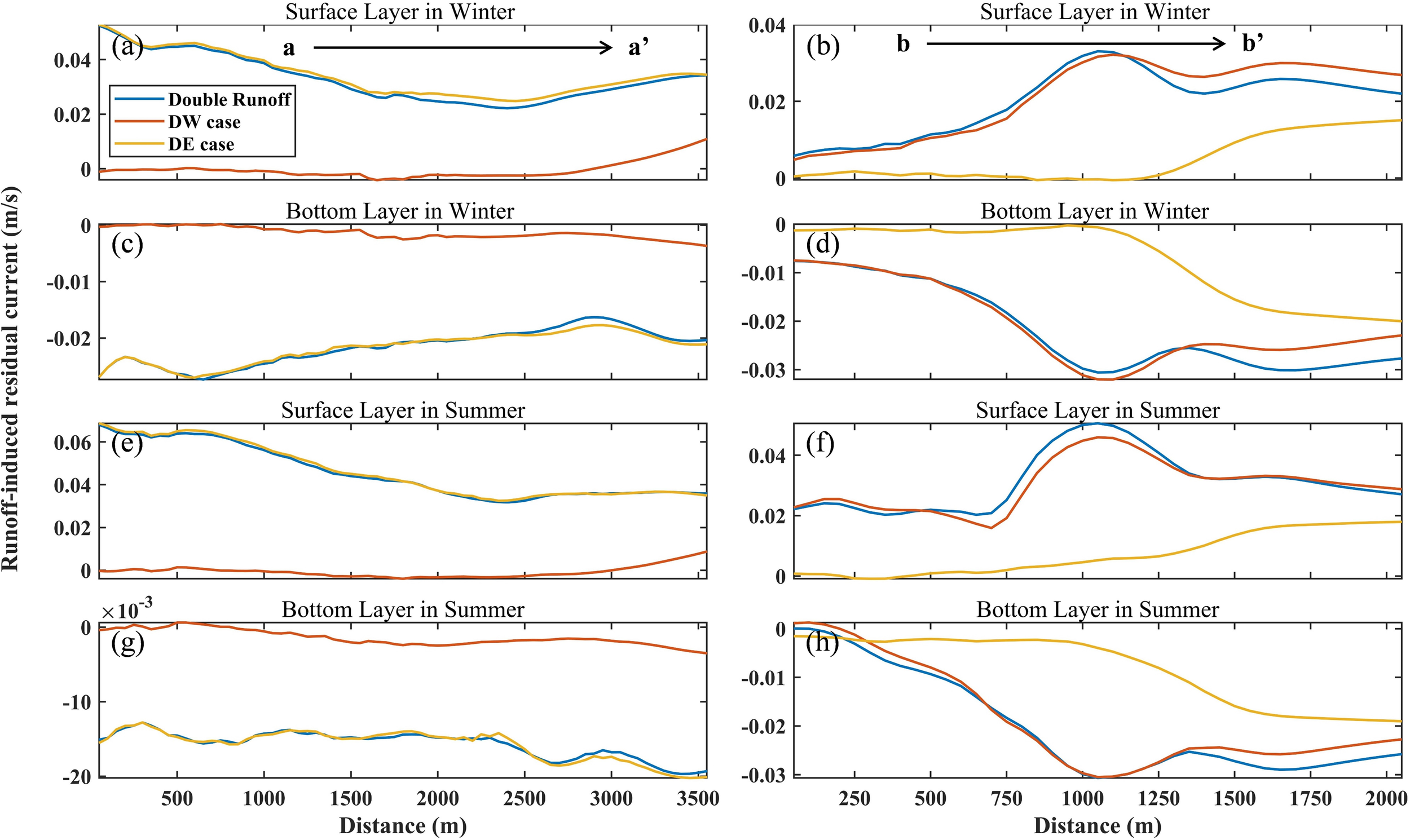
Figure 14. Distribution of runoff-induced residual flow along the profile under different cases. The first column is the a-a’ profile (a, c, e, g), and the second column is the b-b’ profile (b, d, f, h). The blue solid line is the double runoff case runoff-induced residual flow distribution, the orange solid line is the DW case runoff-induced residual flow distribution, and the yellow solid line is the DE case runoff-induced residual flow distribution (+: seaward, –: landward).

To further investigate the influence of waves on runoff-induced residual currents, scatter plots of the runoff residual current with and without waves were drawn at three characteristic points (Figure 15). The red scatter points represent the residual current in both cases, and the black dashed line (y=x) indicates the ideal consistency line, which is used to assess the agreement between the two datasets. The results show that waves exert limited influence on the transverse component of the runoff-induced residual currents (Figure 15a). The scatter points at all three characteristic points are closely aligned with the y=x line with good linear correlations (R² values of 0.93, 0.88, and 0.85, respectively), indicating that the influence of waves on the transverse component of the runoff-induced residual currents is limited. Spatially, point 1 has the highest correlation coefficient and the weakest wave interference, indicating that in open and gently sloping terrain, runoff dominates the hydrodynamics and wave effects are weak. Point 2 is situated in the narrow southern estuary, where terrain constriction and nearshore wave reflection enhance the runoff-wave interaction, leading to a slight decrease in R². Point 3 lies offshore beyond the estuary mouth, where the runoff control weakens and wave influence increases, resulting in more dispersed scatter and further reduced correlation.

Figure 15

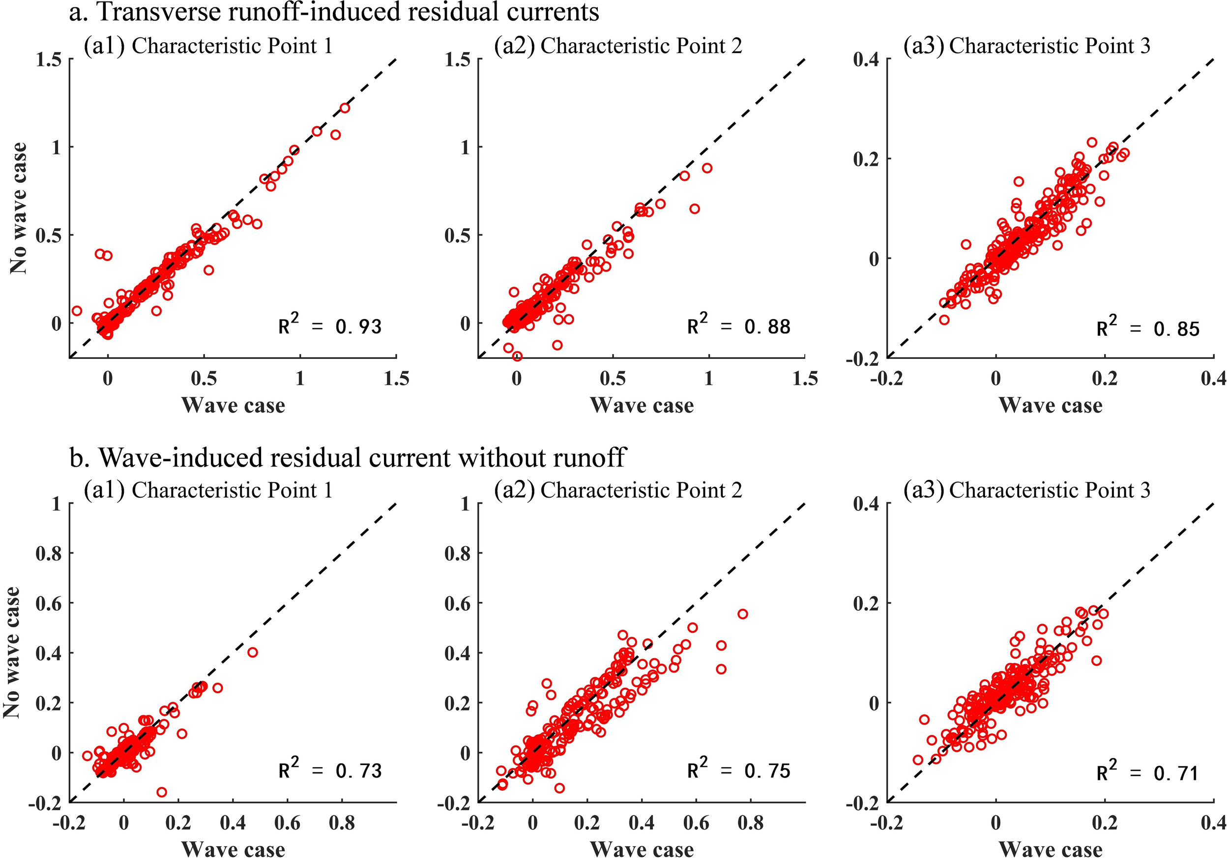
Figure 15. (a) Scatter plot of transverse runoff-induced residual currents under wave and no-wave cases. (b) Scatter plot of longitudinal runoff-induced residual currents under wave and no-wave cases.

The correlation coefficients (R² = 0.73, 0.75, and 0.71, respectively) for the longitudinal component of the residual currents at the three characteristic points are significantly lower than those for the transverse component, indicating that wave-induced disturbances more strongly affect the longitudinal component (Figure 15b). Spatially, point 1 is characterized by gentle topography and a relatively simple hydrodynamic structure. Although influenced by wave action, the longitudinal component retains a relatively high correlation (R² = 0.73), indicating that the runoff-dominated currents remain largely intact, with waves serving a modulatory rather than a reconstructive role. At point 2, the longitudinal component is minimally affected by wave disturbances (R² = 0.75), exhibiting a relatively stable flow response under the coupling of waves and runoff, likely due to channel confinement. The R² of offshore point 3 is only 0.71, indicating that waves exert the strongest modulation on the longitudinal transport of runoff in this area.

Directionally, wave effects are more pronounced on the longitudinal component of residual currents than on the transverse component. Spatially, wave-induced disturbances gradually intensify from the inner estuary toward the offshore area, reflecting the increasing regulatory influence of waves as geomorphic constraints weaken. These directional and spatial patterns highlight the non-uniform modulation of waves on runoff-induced residual currents under varying geomorphic backgrounds.

In summary, the input of runoff significantly enhances seaward and alongshore currents in the estuarine area. The northern estuary runoff has a wide and continuous impact range, while the southern estuary runoff is limited by terrain and has a relatively weak impact. The superposition of double runoff generates spatial heterogeneity, characterized by the coexistence of residual current enhancement and attenuation in different areas. Vertically, the flow field presents a classic estuarine circulation pattern, with surface seaward flow and bottom landward return flow. The influence of waves on runoff-induced residual currents exhibits pronounced directional and spatial variation: transverse disturbances are minor, while longitudinal disturbances are significant, and the regulating effect of waves is strongest in offshore areas.

5 Conclusions

This study investigated the seasonal hydrodynamic processes in the estuary coastal system using a wave-current coupled three-dimensional Delft3D model. Through detailed numerical simulations under various runoff and wave scenarios, we analyzed the seasonal flow field variability and residual current mechanisms, emphasizing the role of runoff-wave coupling and estuarine morphological differences. Main conclusions are as following:

The estuarine hydrodynamics exhibit strong seasonal variability governed primarily by the changes in runoff. During the summer wet season, enhanced runoff leads to intensified seaward transport and stronger alongshore currents, while in the winter dry season, flow velocities are generally weaker and more tidally dominated. The northern estuary, characterized by a wide and gently sloping mouth, shows a more extensive influence range compared to the morphologically constrained southern estuary. The generation and evolution of residual currents are strongly modulated by runoff magnitude and distribution. The inclusion of runoff, especially in the northern estuary, significantly enhances residual currents along the seaward and alongshore directions. The vertical structure of residual flows exhibits a classic estuarine circulation pattern, with surface seaward and bottom landward flows. Notably, the simultaneous presence of two runoff sources produces non-uniform enhancement and cancellation zones, depending on the angular deviation of the jet and the shoreline alignment. Moreover, wave forcing introduces substantial spatial and directional heterogeneity in the residual current field. The transverse components of residual currents remain largely unaffected by waves, but the longitudinal components exhibit significant modulation, particularly in offshore regions where geomorphic constraints are weaker. The correlation analysis reveals a progressively stronger wave influence from the inner estuary to the outer sea, highlighting the non-uniform regulatory role of waves under varying terrain backgrounds.

Overall, this study demonstrates the importance of integrating runoff variability and wave dynamics in the investigation of estuarine hydrodynamic, especially in systems with seasonal freshwater input and complex multi-inlet geometry. The findings provide essential insights into the spatial heterogeneity of residual flows and the interaction mechanisms that sediment transport, stratification, and estuarine exchange processes.

Although this study mainly focuses on hydrodynamic responses to runoff and wave forcing, the findings also have implications for sediment dynamics and morphological evolution. Previous studies in large estuaries, such as the Qiantang Estuary and Yangtze Estuary, have shown that high runoff can enhance bottom shear stress and promote bed erosion during wet seasons or high-flow conditions (Xie et al., 2018; Liu et al., 2020). Similar processes are likely to occur in the present dual-inlet estuary, where increased runoff may alter sediment resuspension and redistribution patterns. Future work will expand the current modeling framework by coupling sediment transport modules to investigate how residual currents modulated by waves and runoff influence sediment redistribution and estuarine morphology. Emphasis will also be placed on simulating extreme events such as typhoons to assess system resilience.

Data availability statement

The raw data supporting the conclusions of this article will be made available by the authors, without undue reservation.

Author contributions

ZZ: Methodology, Software, Validation, Writing – original draft. ZW: Funding acquisition, Investigation, Supervision, Writing – review & editing. BL: Funding acquisition, Methodology, Supervision, Writing – review & editing. YJ: Investigation, Project administration, Writing – review & editing. XL: Investigation, Writing – review & editing. GW: Investigation, Validation, Writing – review & editing.

Funding

The author(s) declare financial support was received for the research and/or publication of this article. The author would like to acknowledge the support of the National Natural Science Foundation of China (No. W2411039), Shandong Offshore Engineering Facility and Material Innovation Entrepreneurship Community (SOFM-IEC) Project (GTP-2504) and the Key R&D Program of Shandong Province, China (2022CXPT004).

Conflict of interest

The authors declare that the research was conducted in the absence of any commercial or financial relationships that could be construed as a potential conflict of interest.

Generative AI statement

The author(s) declare that no Generative AI was used in the creation of this manuscript.

Any alternative text (alt text) provided alongside figures in this article has been generated by Frontiers with the support of artificial intelligence and reasonable efforts have been made to ensure accuracy, including review by the authors wherever possible. If you identify any issues, please contact us.

Publisher’s note

All claims expressed in this article are solely those of the authors and do not necessarily represent those of their affiliated organizations, or those of the publisher, the editors and the reviewers. Any product that may be evaluated in this article, or claim that may be made by its manufacturer, is not guaranteed or endorsed by the publisher.

Supplementary material

The Supplementary Material for this article can be found online at: https://www.frontiersin.org/articles/10.3389/fmars.2025.1707930/full#supplementary-material

References

Cheng P., Valle-Levinson A., and De Swart H. E. (2010). Residual currents induced by asymmetric tidal mixing in weakly stratified narrow estuaries. J. Phys. oceanogr. 40, 2135–2147. doi: 10.1175/2010JPO4314.1

Crossref Full Text | Google Scholar

Deltares (2014). “Delft3d-flow user manual (version: 3.15. 34158): Simulation of multi-dimensional hydrodynamic flows and transport phenomena, including sediments,” in Delft3D-FLOW user manual (Version: 3.15). (The Netherlands: Deltares).

Google Scholar

Ding Y. and Wang S. S. (2008). Development and application of a coastal and estuarine morphological process modeling system. J. Coast. Res. 2008 (10052), 127–140. doi: 10.2112/1551-5036-52.sp1.127

Crossref Full Text | Google Scholar

Dissanayake P., Brown J., and Karunarathna H. (2014). Modelling storm-induced beach/dune evolution: Sefton coast, liverpool bay, uk. Mar. Geol. 357, 225–242. doi: 10.1016/j.margeo.2014.07.013

Crossref Full Text | Google Scholar

Dissanayake D., Wurpts A., Miani M., Knaack H., Niemeyer H., and Roelvink J. (2012). Modelling morphodynamic response of a tidal basin to an anthropogenic effect: Ley bay, east frisian wadden sea–applying tidal forcing only and different sediment fractions. Coast. Eng. 67, 14–28. doi: 10.1016/j.coastaleng.2012.04.001

Crossref Full Text | Google Scholar

Dyer K. and Ramamoorthy K. (1969). Salinity and water circulation in the vellar estuary. Limnol. Oceanogr. 14, 4–15. doi: 10.4319/lo.1969.14.1.0004

Crossref Full Text | Google Scholar

Gao J., Hou L., Liu Y., and Shi H. (2024). Influences of bragg reflection on harbor resonance triggered by irregular wave groups. Ocean Eng. 305, 117941. doi: 10.1016/j.oceaneng.2024.117941

Crossref Full Text | Google Scholar

Gao L., Li D.-J., and Ding P.-X. (2009). Quasi-simultaneous observation of currents, salinity and nutrients in the changjiang (yangtze river) plume on the tidal timescale. J. Mar. Syst. 75, 265–279. doi: 10.1016/j.jmarsys.2008.10.006

Crossref Full Text | Google Scholar

Gao J., Ma X., Dong G., Chen H., Liu Q., and Zang J. (2021). Investigation on the effects of bragg reflection on harbor oscillations. Coast. Eng. 170, 103977. doi: 10.1016/j.coastaleng.2021.103977

Crossref Full Text | Google Scholar

Gao J., Ma X., Zang J., Dong G., Ma X., Zhu Y., et al. (2020). Numerical investigation of harbor oscillations induced by focused transient wave groups. Coast. Eng. 158, 103670. doi: 10.1016/j.coastaleng.2020.103670

Crossref Full Text | Google Scholar

Gao J., Shi H., Zang J., and Liu Y. (2023). Mechanism analysis on the mitigation of harbor resonance by periodic undulating topography. Ocean Eng. 281, 114923. doi: 10.1016/j.oceaneng.2023.114923

Crossref Full Text | Google Scholar

Geyer W. R. and MacCready P. (2014). The estuarine circulation. Annu. Rev. fluid mechanics 46, 175–197. doi: 10.1146/annurev-fluid-010313-141302

Crossref Full Text | Google Scholar

Green M. O. and Coco G. (2014). Review of wave-driven sediment resuspension and transport in estuaries. Rev. Geophysics 52, 77–117. doi: 10.1002/2013RG000437

Crossref Full Text | Google Scholar

He W., Jiang A., Zhang J., Xu H., Xiao Y., Chen S., et al. (2021). Hydrodynamic characteristics of lateral withdrawal in a tidal river channel with saltwater intrusion. Ocean Eng. 228, 108905. doi: 10.1016/j.oceaneng.2021.108905

Crossref Full Text | Google Scholar

Hersbach H., Bell B., Berrisford P., Hirahara S., Horányi A., Muñoz-Sabater J., et al. (2020). The era5 global reanalysis. Q. J. R. meteorological Soc. 146, 1999–2049. doi: 10.1002/qj.3803

Crossref Full Text | Google Scholar

Hu K., Ding P., Wang Z., and Yang S. (2009). A 2d/3d hydrodynamic and sediment transport model for the yangtze estuary, China. J. Mar. Syst. 77, 114–136. doi: 10.1016/j.jmarsys.2008.11.014

Crossref Full Text | Google Scholar

Hughes F. and Rattray M. Jr. (1980). Salt flux and mixing in the columbia river estuary. Estuar. Coast. Mar. Sci. 10, 479–493. doi: 10.1016/S0302-3524(80)80070-3

Crossref Full Text | Google Scholar

Jay D. A. and Smith J. D. (1990). Residual circulation in shallow estuaries: 2. weakly stratified and partially mixed, narrow estuaries. J. Geophysical Research: Oceans 95, 733–748. doi: 10.1029/JC095iC01p00733

Crossref Full Text | Google Scholar

Kim T., Choi B., and Lee S. (2006). Hydrodynamics and sedimentation induced by large-scale coastal developments in the keum river estuary, korea. Estuarine Coast. Shelf Sci. 68, 515–528. doi: 10.1016/j.ecss.2006.03.003

Crossref Full Text | Google Scholar

Kuang C., Liu X., Gu J., Guo Y., Huang S., Liu S., et al. (2013). Numerical prediction of medium-term tidal flat evolution in the yangtze estuary: Impacts of the three gorges project. Continental Shelf Res. 52, 12–26. doi: 10.1016/j.csr.2012.10.006

Crossref Full Text | Google Scholar

Lerczak J. A., Geyer W. R., and Chant R. J. (2006). Mechanisms driving the time-dependent salt flux in a partially stratified estuary. J. Phys. Oceanogr. 36, 2296–2311. doi: 10.1175/JPO2959.1

Crossref Full Text | Google Scholar

Li C. and O’Donnell J. (2005). The effect of channel length on the residual circulation in tidally dominated channels. J. Phys. Oceanogr. 35, 1826–1840. doi: 10.1175/JPO2804.1

Crossref Full Text | Google Scholar

Liu H. (2011). Fate of three major rivers in the bohai sea: A model study. Continental Shelf Res. 31, 1490–1499. doi: 10.1016/j.csr.2011.06.013

Crossref Full Text | Google Scholar

Liu X. J., Kettner A. J., Cheng J., and Dai S. (2020). Sediment characteristics of the yangtze river during major flooding. J. Hydrol. 590, 125417. doi: 10.1016/j.jhydrol.2020.125417

Crossref Full Text | Google Scholar

Luan H. L., Ding P. X., Wang Z. B., Ge J. Z., and Yang S. L. (2016). Decadal morphological evolution of the yangtze estuary in response to river input changes and estuarine engineering projects. Geomorphology 265, 12–23. doi: 10.1016/j.geomorph.2016.04.022

Crossref Full Text | Google Scholar

Matsumoto K., Takanezawa T., and Ooe M. (2000). Ocean tide models developed by assimilating topex/poseidon altimeter data into hydrodynamical model: A global model and a regional model around Japan. J. oceanogr. 56, 567–581. doi: 10.1023/A:1011157212596

Crossref Full Text | Google Scholar

Mayerle R., Narayanan R., Etri T., and Abd Wahab A. K. (2015). A case study of sediment transport in the paranagua estuary complex in Brazil. Ocean Eng. 106, 161–174. doi: 10.1016/j.oceaneng.2015.06.025

Crossref Full Text | Google Scholar

Mellor G. (2003). The three-dimensional current and surface wave equations. J. Phys. oceanogr. 33, 1978–1989. doi: 10.1175/1520-0485(2003)033<1978:TTCASW>2.0.CO;2

Crossref Full Text | Google Scholar

Meyers S. D., Linville A. J., and Luther M. E. (2014). Alteration of residual circulation due to large-scale infrastructure in a coastal plain estuary. Estuaries Coasts 37, 493–507. doi: 10.1007/s12237-013-9691-3

Crossref Full Text | Google Scholar

Miguel L. L. A. J., Castro J. W. A., and Nehama F. P. J. (2017). Tidal impact on suspended sediments in the macuse estuary in Mozambique. Regional Stud. Mar. Sci. 16, 1–14. doi: 10.1016/j.rsma.2017.07.002

Crossref Full Text | Google Scholar

Moon J.-H., Hirose N., Yoon J.-H., and Pang I.-C. (2010). Offshore detachment process of the low- salinity water around changjiang bank in the east China sea. J. Phys. Oceanogr. 40, 1035–1053. doi: 10.1175/2010JPO4167.1

Crossref Full Text | Google Scholar

Moriasi D. N., Arnold J. G., Van Liew M. W., Bingner R. L., Harmel R. D., and Veith T. L. (2007). Model evaluation guidelines for systematic quantification of accuracy in watershed simulations. Trans. ASABE 50, 885–900. doi: 10.13031/2013.23153

Crossref Full Text | Google Scholar

Nienhuis J. H., Ashton A. D., Edmonds D. A., Hoitink A., Kettner A. J., Rowland J. C., et al. (2020). Global-scale human impact on delta morphology has led to net land area gain. Nature 577, 514–518. doi: 10.1038/s41586-019-1905-9

PubMed Abstract | Crossref Full Text | Google Scholar

Olabarrieta M., Medina R., and Castanedo S. (2010). Effects of wave–current interaction on the current profile. Coast. Eng. 57, 643–655. doi: 10.1016/j.coastaleng.2010.02.003

Crossref Full Text | Google Scholar

Olabarrieta M., Warner J. C., and Kumar N. (2011). Wave-current interaction in willapa bay. J. Geophysical Research: Oceans 116, C12. doi: 10.1029/2011JC007387

Crossref Full Text | Google Scholar

Palma E. D. and Matano R. P. (2012). A numerical study of the magellan plume. J. Geophysical Research: Oceans 117, C5.

Google Scholar

Roberts W., Le Hir P., and Whitehouse R. (2000). Investigation using simple mathematical models of the effect of tidal currents and waves on the profile shape of intertidal mudflats. Continental Shelf Res. 20, 1079–1097. doi: 10.1016/S0278-4343(00)00013-3

Crossref Full Text | Google Scholar

Sánchez M., Carballo R., Ramos V., and Iglesias G. (2014). Tidal stream energy impact on the transient and residual flow in an estuary: A 3d analysis. Appl. Energy 116, 167–177. doi: 10.1016/j.apenergy.2013.11.052

Crossref Full Text | Google Scholar

Scully M. E., Friedrichs C., and Brubaker J. (2005). Control of estuarine stratification and mixing by wind-induced straining of the estuarine density field. Estuaries 28, 321–326. doi: 10.1007/BF02693915

Crossref Full Text | Google Scholar

Simpson J., Bos W., Schirmer F., Souza A., Rippeth T., Jones S., et al. (1993). Periodic stratification in the rhine rofi in the north-sea. Oceanologica Acta 16, 23–32. Available online at: https://archimer.ifremer.fr/doc/00099/21050/.

Google Scholar

Sylaios G. and Boxall S. (1998). Residual currents and flux estimates in a partially-mixed estuary. Estuarine Coast. Shelf Sci. 46, 671–682. doi: 10.1006/ecss.1997.0312

Crossref Full Text | Google Scholar

Twigt D. J., De Goede E. D., Zijl F., Schwanenberg D., and Chiu A. Y. (2009). Coupled 1d–3d hydrodynamic modelling, with application to the pearl river delta. Ocean Dynamics 59, 1077–1093. doi: 10.1007/s10236-009-0229-y

Crossref Full Text | Google Scholar

Van der Wegen M. and Roelvink J. (2012). Reproduction of estuarine bathymetry by means of a process-based model: Western scheldt case study, the Netherlands. Geomorphology 179, 152–167. doi: 10.1016/j.geomorph.2012.08.007

Crossref Full Text | Google Scholar

Wang Q., Guo X., and Takeoka H. (2008). Seasonal variations of the yellow river plume in the bohai sea: A model study. J. Geophysical Research: Oceans 113, C8. doi: 10.1029/2007JC004555

Crossref Full Text | Google Scholar

Wang J., Li L., He Z., Kalhoro N. A., and Xu D. (2019). Numerical modelling study of seawater intrusion in indus river estuary, Pakistan. Ocean Eng. 184, 74–84. doi: 10.1016/j.oceaneng.2019.05.029

Crossref Full Text | Google Scholar

Wolf J. and Prandle D. (1999). Some observations of wave–current interaction. Coast. Eng. 37, 471–485. doi: 10.1016/S0378-3839(99)00039-3

Crossref Full Text | Google Scholar

Wu H. and Zhu J. (2010). Advection scheme with 3rd high-order spatial interpolation at the middle temporal level and its application to saltwater intrusion in the changjiang estuary. Ocean Model. 33, 33–51. doi: 10.1016/j.ocemod.2009.12.001

Crossref Full Text | Google Scholar

Xie D. F., Gao S., Wang Z. B., and Pan C. H. (2013). Numerical modeling of tidal currents, sediment transport and morphological evolution in hangzhou bay, China. Int. J. Sediment Res. 28, 316–328. doi: 10.1016/S1001-6279(13)60042-6

Crossref Full Text | Google Scholar

Xie D. F., Gao S., Wang Z. B., Pan C. H., Wu X. G., and Wang Q. S. (2017). Morphodynamic modeling of a large inside sandbar and its dextral morphology in a convergent estuary: Qiantang estuary, China. J. Geophysical Research: Earth Surface 122, 1553–1572. doi: 10.1002/2017JF004293

Crossref Full Text | Google Scholar

Xie D., Pan C., Gao S., and Wang Z. B. (2018). Morphodynamics of the qiantang estuary, China: Controls of river flood events and tidal bores. Mar. Geol. 406, 27–33. doi: 10.1016/j.margeo.2018.09.003

Crossref Full Text | Google Scholar

Yu Q., Wang Y., Shi B., Wang Y. P., and Gao S. (2017). Physical and sedimentary processes on the tidal flat of central Jiangsu coast, China: Headland induced tidal eddies and benthic fluid mud layers. Continental Shelf Res. 133, 26–36. doi: 10.1016/j.csr.2016.12.015

Crossref Full Text | Google Scholar

Yuan B., Sun J., Lin B., and Zhang F. (2020). Long-term morphodynamics of a large estuary subject to decreasing sediment supply and sea level rise. Global Planetary Change 191, 103212. doi: 10.1016/j.gloplacha.2020.103212

Crossref Full Text | Google Scholar

Zhang Z., Liang B., Wang Z., Shi L., and Borsje B. (2024). Effects of wave forces on sediment transport patterns in micro-tidal estuaries. Phys. Fluids 36, 2. doi: 10.1063/5.0187839

Crossref Full Text | Google Scholar

Zhang X., Simons R., Zheng J., and Zhang C. (2022). A review of the state of research on wave-current interaction in nearshore areas. Ocean Eng. 243, 110202. doi: 10.1016/j.oceaneng.2021.110202

Crossref Full Text | Google Scholar

Zhou X., Zheng J., Doong D.-J., and Demirbilek Z. (2013). Sea level rise along the east asia and Chinese coasts and its role on the morphodynamic response of the yangtze river estuary. Ocean Eng. 71, 40–50. doi: 10.1016/j.oceaneng.2013.03.014

Crossref Full Text | Google Scholar

Zhu J., Weisberg R. H., Zheng L., and Han S. (2015). Influences of channel deepening and widening on the tidal and nontidal circulations of tampa bay. Estuaries Coasts 38, 132–150. doi: 10.1007/s12237-014-9815-4

Crossref Full Text | Google Scholar