Spring-neap variation of total suspended solids over the Changjiang Bank in winter based on GOCI

Total suspended solids concentration (TSS) over the Changjiang Bank exhibits significant spatial heterogeneity and distinct rhythmic variations at spring-neap and quarter-diurnal timescales. However, limited spatial coverage of observations restricts large-area TSS mapping, while insufficient temporal resolution introduces frequency aliasing that obscures spring-neap TSS signatures. Here, we applied spatiotemporal Kriging interpolation to hourly TSS data from the Geostationary Ocean Color Imager (GOCI) to enhance spatial coverage. Subsequently, the daily mean (TSS_daily) and daily range (ΔTSS) of TSS were derived to quantitatively analyze the spatiotemporal evolution of TSS over a spring-neap cycle. Results show that both TSS_daily and ΔTSS present a tongue-shaped distribution decreasing southeastward, which can be classified into high-, medium-, and low-turbidity & diurnal-variability zones offshore (denoted as H-, M-, and L-Zones). Notably, the H-Zone displays a stepped pattern aligned with three latitudinal sand dunes near the 40-m isobath. Over the spring-neap cycle, TSS_daily and ΔTSS generally co-varied with tidal currents. The H-Zone contracted and gradually lost its stepped pattern as tidal currents weakened, then expanded and reestablished this stepped pattern as tidal currents strengthened. Mechanistic analysis reveals that the spatiotemporal variations in TSS_daily and ΔTSS are primarily governed by tide-induced mixing, modulated by water depth and tidal currents velocity. Specifically, water depth determines their distribution patterns, while variations in tidal current velocity drive their spring-neap evolution.

1 Introduction

The Changjiang Bank (122°–126.5°E, 30.5°–34°N) is situated at the junction of the Yellow Sea and the East China Sea (YECS) (Figure 1a), and features a relatively flat topography with an average depth of ~26 m (Zhou et al., 2020a). Dominated by the M₂ tidal constituent, this region exhibits typical semi-diurnal tidal characteristics, with strong tidal dynamics (Lie et al., 2002; Xuan et al., 2016) (Figure 1b), which provide the primary driving force for sediment resuspension and transport. Spatially, the total suspended solids (TSS) concentrations are generally higher in coastal areas than in the open sea. Temporally, TSS variability is co-modulated by hydrodynamics (e.g., tides, wind waves) and atmospheric forcing (e.g., monsoons, cooling), exhibiting multi-scale variations. Among these, seasonal variability is the most pronounced, characterized by a distinct “highest in winter and lowest in summer” pattern (Yuan et al., 2008; Shi and Wang, 2010; Shi et al., 2011a; Luo et al., 2017; Zhou et al., 2020a, 2020b). In winter (from January to March), strong monsoons and cooling disrupt water column stratification, while intense tidal mixing drives large-scale resuspension of fine-grained sediments, forming a turbid plume extending from the Jiangsu coast to the southeastern open sea (Figure 1c). This makes the Changjiang Bank one of the most turbid coastal areas in the world (Milliman and Meade, 1983; Shi and Wang, 2010; Luo et al., 2017).

Figure 1

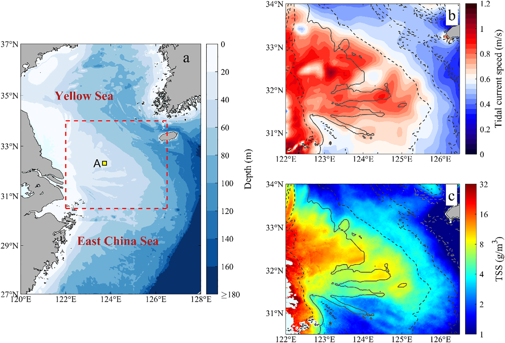
Figure 1. (a) Location and bathymetry of the study area, the red dashed box denotes the study area (122°–126.5°E, 30.5°–34°N), and the yellow rectangle marks the location of Area A (a 2.5×2.5 km² region centered at 123.7°E, 32.3°N); (b) Distribution of tidal current velocity amplitude; (c) Distribution of average TSS in the winter of 2020 based on GOCI, the solid line represents the 40-m isobath, and the dashed lines represent the 20-, 60-, 80-, and 100-m isobaths respectively in (b) and (c).

Regulated by periodic tidal motions, TSS concentration also exhibits significant tidal rhythmicity: in response to the semi-diurnal cycle (12.4 h), where current velocity peaks twice, accordingly TSS shows high-frequency quarter-diurnal variations with a period of 6.2 h; additionally, due to the phase superposition of M₂ and S₂ tidal constituents, TSS also presents low-frequency spring-neap variations (Chen, 2001; Yang et al., 2004; Shi et al., 2011a; Luo et al., 2017; Zhou et al., 2017, 2020a, 2020b). However, due to limitations in the spatial coverage and temporal resolution of existing observation methods, systematic quantitative research on the spatiotemporal evolution of TSS and the underlying mechanisms at the spring-neap scale remains inadequate.

Based on high-frequency in-situ observations, Chen (2001) found that TSS concentration in the Yangtze Estuary during spring tides could reach 1.5–2.5 times that during neap tide. Souza et al. (2004) and Yang et al. (2004) further revealed that, driven by semi-diurnal tides, TSS concentration also exhibits high-frequency quarter-diurnal fluctuations superimposed on spring-neap variability. Notably, the amplitude of this high-frequency signal is also modulated by the spring-neap cycle, to the extent that during spring tides, it can rival the magnitude of the spring-neap variability. However, restricted to single-point or local coverage, in-situ observations fail to reveal the large-area spatiotemporal evolution of TSS at both spring-neap and quarter-diurnal scales (Fettweis et al., 2019; Lin et al., 2022).

Remote sensing, leveraging its advantages of large-area and long-term observations, has gradually become the primary tool for investigating multi-scale spatiotemporal variations of TSS (He et al., 2013; Zhou et al., 2017, 2020a, 2020b; Du et al., 2025). Studies based on lunar-phase-averaged polar-orbiting satellite data have revealed significant spring-neap TSS variations over the Bohai, Yellow, and East China Sea shelf, with amplitudes decreasing offshore—consistent with the spatial distribution of mean TSS concentration (Shi et al., 2011a; Zhou et al., 2017, 2020b). However, the once-daily sampling frequency of polar-orbiting satellites is insufficient to resolve TSS quarter-diurnal signals. This limitation may lead to high-frequency quarter-diurnal fluctuations being misinterpreted as spring-neap trends, thereby distorting the extraction of spring-neap TSS signatures.

Marine observation essentially involves discrete sampling of spatiotemporally continuous signals, and its accuracy is strictly constrained by sampling frequency and duration. According to the Nyquist-Shannon theorem, accurate resolution of multi-frequency signals requires satisfying two conditions simultaneously: first, the sampling frequency ($f_s$​) must be at least twice the highest-frequency signal ($f_{high}$), i.e., $f_s>2f_{high}$, to avoid aliasing; second, the sampling duration ($T_s$) must cover at least one full cycle of the lowest-frequency signal ($T_{low}$), i.e., $T_s$> $T_{low}$, to fully capture its periodic variation (Emery and Thomson, 2001; Wang et al., 2022). For TSS dynamics in semi-diurnal tidal regions, which exhibit both low-frequency spring-neap signals (with a period of ~15 d) and high-frequency quarter-diurnal signals (with a period of ~6.2 h), the sampling strategy must theoretically achieve a temporal resolution finer than 3.1 h and a duration of no less than 15 d.

The world’s first geostationary ocean color imager (GOCI), launched in 2010, has significantly enhanced observational capabilities. Its eight hourly samplings from 08:16 to 15:16 (local time) can evenly cover one full quarter-diurnal TSS cycle. Additionally, its hourly sampling frequency meets the required Nyquist frequency. In a comparative study of satellites with different revisit cycles (e.g., GOCI, MODIS, Sentinel, and Landsat), Lin et al. (2022) demonstrated that only GOCI can capture TSS diurnal signals, with significantly superior accuracy in multi-scale feature extraction. Leveraging this advantage, subsequent studies have further revealed that TSS in shelf seas exhibits intense quarter-diurnal variation driven by tidal mixing, and have quantitatively characterized its spatiotemporal variability (Zhou et al., 2020a; Du et al., 2021; Li et al., 2021).

However, the practical application of GOCI remains limited. Firstly, cloud cover frequently results in extensive data gaps in hourly observations, making it challenging to capture the full spatial patterns of TSS. Previous studies have predominantly relied on selecting individual days with eight consecutive hourly GOCI images that exhibit optimal spatiotemporal coverage, comparing average TSS distributions across different tidal phases (Du et al., 2021; Li et al., 2021). This approach, however, cannot investigate the continuous spatiotemporal evolution of TSS over a spring-neap cycle. Secondly, tidal asymmetry induces significant diurnal inequality in the intensity of quarter-diurnal TSS variations (Yang et al., 2004), while GOCI captures only one quarter-diurnal cycle per day. Therefore, whether GOCI-derived mean values can reasonably represent the daily average state of TSS remains to be rigorously validated.

In summary, effectively integrating fragmented GOCI data to enhance spatial coverage and extract more representative spring-neap TSS signatures has become a critical issue. To address this, we applied spatiotemporal Kriging interpolation (ST-Kriging) to hourly GOCI observations, thereby improving spatial coverage. Subsequently, the daily mean and daily range of TSS were derived from the reconstructed data, representing the daily average level and diurnal variability of TSS, respectively. On this basis, we quantitatively analyzed the spatiotemporal evolution of TSS over the Changjiang Bank in winter over a spring-neap cycle. Furthermore, by incorporating high-precision bathymetric data and tidal current simulations from the Finite Volume Community Ocean Model (FVCOM), we preliminarily explored the underlying dynamic mechanisms from the perspective of tide-induced mixing.

2 Materials and methods

2.1 Materials

2.1.1 Hourly TSS data from GOCI

Hourly TSS data used in this study were derived from GOCI, provided by the Korea Ocean Satellite Center (KOSC). From April 2011 to March 2021, GOCI continuously monitored an area of ~2500×2500 km² centered on the Korean Peninsula (36°N, 130°E), delivering hourly TSS data (referred to as GOCI-TSS) with a spatial resolution of 500 m from 08:16 to 15:16 local time (Cho et al., 2010; Choi et al., 2012; Wang et al., 2013, 2023). Validation has confirmed that the official TSS products retrieved from the Yellow Sea Large Marine Ecosystem Ocean Color (YOC) algorithm performs well over the YECS (Siswanto et al., 2011), and have been widely used in studies investigating the spatiotemporal dynamics of TSS in this region (Zhou et al., 2020a, 2020b). By reviewing winter GOCI-TSS imagery from 2012 to 2021, hourly data from March 11 to 25, 2020 (excluding March 13 and 22 due to cloud cover) with good spatiotemporal continuity were selected for analyzing spring-neap TSS variations.

The tidal rhythmicity in TSS is primarily driven by tidal energy dissipation (Souza et al., 2004; Yu et al., 2011, 2012). Theoretically, under the assumption that TSS varies synchronously with tidal motion, its magnitude is proportional to the cube of tidal current velocity (U³). Hence, the periodic variation of U³ can be used to approximate the variation pattern of TSS. This study takes Area A on the Changjiang Bank (location shown in Figure 1a) as a representative site to elucidate the strengths and limitations of GOCI in resolving spring-neap TSS variations. This is achieved by comparing the similarities and differences between the actual daily mean and daily range of U³ and those derived from GOCI’s eight hourly sampling instances over a spring-neap cycle (Figure 2). For quantitative assessment, the Mean Relative Error (MRE) is adopted to evaluate the numerical difference, and the coefficient of determination (R²) is used to measure the consistency of variation trends.

Figure 2

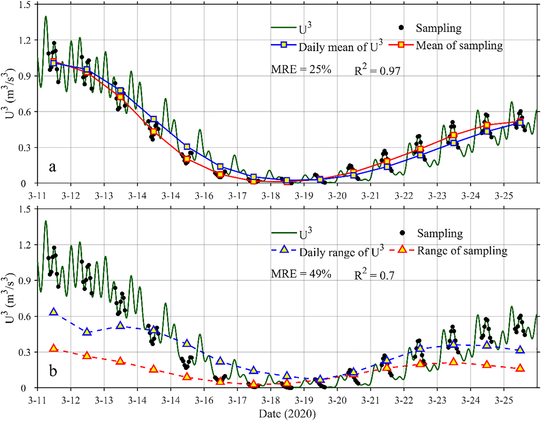
Figure 2. Comparison between the actual cubed tidal current velocity (U³) and U³ values at GOCI sampling instances in Area A (March 11–25, 2020): (a) U³ mean; (b) U³ range. The green solid lines represent U³ time series, and black dots denote GOCI hourly sampling points (08:16–15:16). In (a), the solid blue rectangle represents the daily mean of U³; solid red rectangle represents the mean of U³ during the GOCI sampling period. In (b), the dashed blue triangle represents the daily range of U³; the dashed red triangle represents the range of U³ during the GOCI sampling period.

The results indicate that although GOCI’s 8-hour observation window covers one quarter-diurnal cycle (6.2 h) of U³, the intensity of U³ quarter-diurnal variation exhibits significant intra-day differences due to tidal asymmetry. This leads to discrepancies between the GOCI-sampled mean and range of U³ and the actual daily mean and daily range of U³.

For the U³ mean (Figure 2a), the MRE between the GOCI-sampled mean U³ and the actual daily mean U³ is 25%. However, the relative difference in the amplitude of spring-neap variation reflected by the two is only about 2.8%, which is negligible. Moreover, their variation trends are highly consistent (R²=0.97), with complete synchronization in the timing of peaks and troughs. Thus, it can be inferred that, the GOCI-derived TSS mean more accurately reflects both the amplitude and phase characteristics of the TSS daily mean over the spring-neap cycle than the once-daily sampling by polar-orbiting satellites.

For the U³ range (Figure 2b), the GOCI-sampled U³ range significantly underestimates the actual daily U³ range, with an MRE as high as 49%, and the relative error in the extracted spring-neap amplitude is 47%. Additionally, the consistency in variation trends and phase synchronization between them is slightly reduced compared to those of the daily U³ mean. Nonetheless, R² between them remains 0.7. In contrast to polar-orbiting satellites, which cannot capture diurnal variations in TSS, GOCI is still able to capture the main spring-neap variation trend in the TSS daily range, thereby providing valuable reference for research on spring-neap dynamics of TSS daily range.

2.1.2 Tidal currents from FVCOM

Tidal currents are the major source of kinetic energy on the continental shelf of the YECS, and their periodic motion directly drives quarter-diurnal and spring-neap variations in TSS (Shi et al., 2011a; He et al., 2013; Zhou et al., 2017, 2020a, 2020b; Du et al., 2021). This study uses high-resolution FVCOM tidal current simulations from Xuan et al. (2016), which have a spatial resolution of approximately 1 km and a time interval of 1 h. The model incorporates eight dominant tidal constituents (M₂, S₂, K₁, O₁, N₂, P₁, K₂, Q₁) of the Changjiang Bank. The simulated results, which have been validated in previous studies, can reasonably reflect the realistic tidal currents in this region. Harmonic analysis was performed on the simulated tidal currents using the MATLAB toolbox T_Tide (Pawlowicz et al., 2002) to obtain the harmonic constants (phase φ and amplitude A) of each tidal constituent, followed by prediction of hourly tidal currents during satellite observations.

2.1.3 Bathymetry data

The spatial pattern of surface TSS concentration in shelf seas exhibits similarities to seabed topographic features (Shi et al., 2011b; Mao et al., 2016; Zhou et al., 2020a). Thus, high-precision bathymetric data are crucial for accurate analysis of TSS spatial patterns. This study utilizes high-precision bathymetry data provided by the Qingdao Institute of Marine Geology, China Geological Survey (Kong et al., 2022). Compared with existing global high-resolution bathymetric data, this data better displays fine-scale geomorphic features of the Changjiang Bank.

2.2 Methods

2.2.1 TSS data reconstruction using ST-Kriging

Hourly GOCI-TSS data contain extensive gaps due to cloud cover, which not only introduces uneven intervals in the observed TSS time series, hindering the extraction of spring-neap TSS signatures, but also results in insufficient spatial coverage, making it difficult to capture the spatial pattern of TSS. To address this, this study employed ST-Kriging to interpolate the missing data in the hourly TSS images. This method comprehensively utilizes the spatiotemporal correlation of TSS data from adjacent regions and adjacent time points, significantly improving interpolation accuracy compared to unidimensional (spatial or temporal only) approaches, and is particularly suitable for reconstructing spatiotemporal dynamic in regional scale (Bargaoui and Chebbi, 2009; Xu et al., 2011; Kilibarda et al., 2014).

To further improve interpolation accuracy, this study utilized five days of hourly GOCI-TSS data with optimal spatiotemporal coverage during the winter of 2020 (February 20, 23, and March 8, 20, 31). From these data, 20% of the valid pixels were randomly selected as a test dataset to evaluate the variability of TSS concentration under different spatiotemporal windows and the influence of valid data quantity on the ST-Kriging performance. First, by calculating the coefficient of variation (CV, i.e., the ratio of standard deviation to the mean, Figure 3a) of TSS concentration within different spatiotemporal windows, it was found that the variability increased significantly as the windows expanded. Based on this pattern, a CV of 9% was set as the critical threshold for determining spatiotemporal consistency of TSS concentration, under which the TSS distribution within the corresponding window is considered relatively uniform. After balancing data availability and interpolation accuracy, the optimal interpolation window was determined to be 11×11 pixels (spatial) × 3 h (temporal). Furthermore, the impact of valid data quantity on interpolation accuracy was assessed by analyzing the normalized RMSE (i.e., the ratio of RMSE to the observed value, Figure 3b). The results showed that interpolation accuracy improved significantly as the amount of valid data increased. When the number of valid pixels exceeded 20% (i.e., 72 pixels) of the total pixels in the 11×11×3 window, the normalized RMSE fell below 0.01, indicating relatively accurate interpolation results.

Figure 3

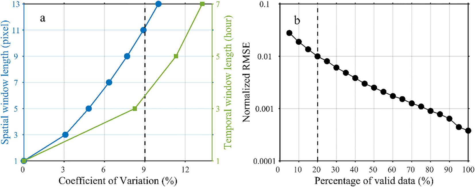
Figure 3. (a) Average coefficient of variation of TSS concentration within spatial or temporal windows of different lengths; (b) Normalized RMSE of interpolation results under different valid data volumes.

Based on the above parameters, the interpolation process for hourly TSS data proceeds as follows: First, data preprocessing is conducted to remove outliers (TSS ≤ 0 g/m³ or TSS>100 g/m³), and a 3×3 pixels Gaussian filter (standard deviation σ=1 pixel) is applied for smoothing. Subsequently, for each invalid pixel in the hourly TSS distribution, if the percentage of valid data within its 11×11×3 window exceeds 20%, the MATLAB DACE toolbox (Lophaven et al., 2002) is used to perform ST-Kriging on the invalid pixel. The reconstruction results show a significant improvement in the spatial coverage of hourly TSS (Figures 4a, b), as well as a notable increase in the cumulative amount of valid data over the Changjiang Bank during the observation period (Figures 4c, d), facilitating a more precise characterization of large-scale TSS spatial patterns and its spring-neap variability.

Figure 4

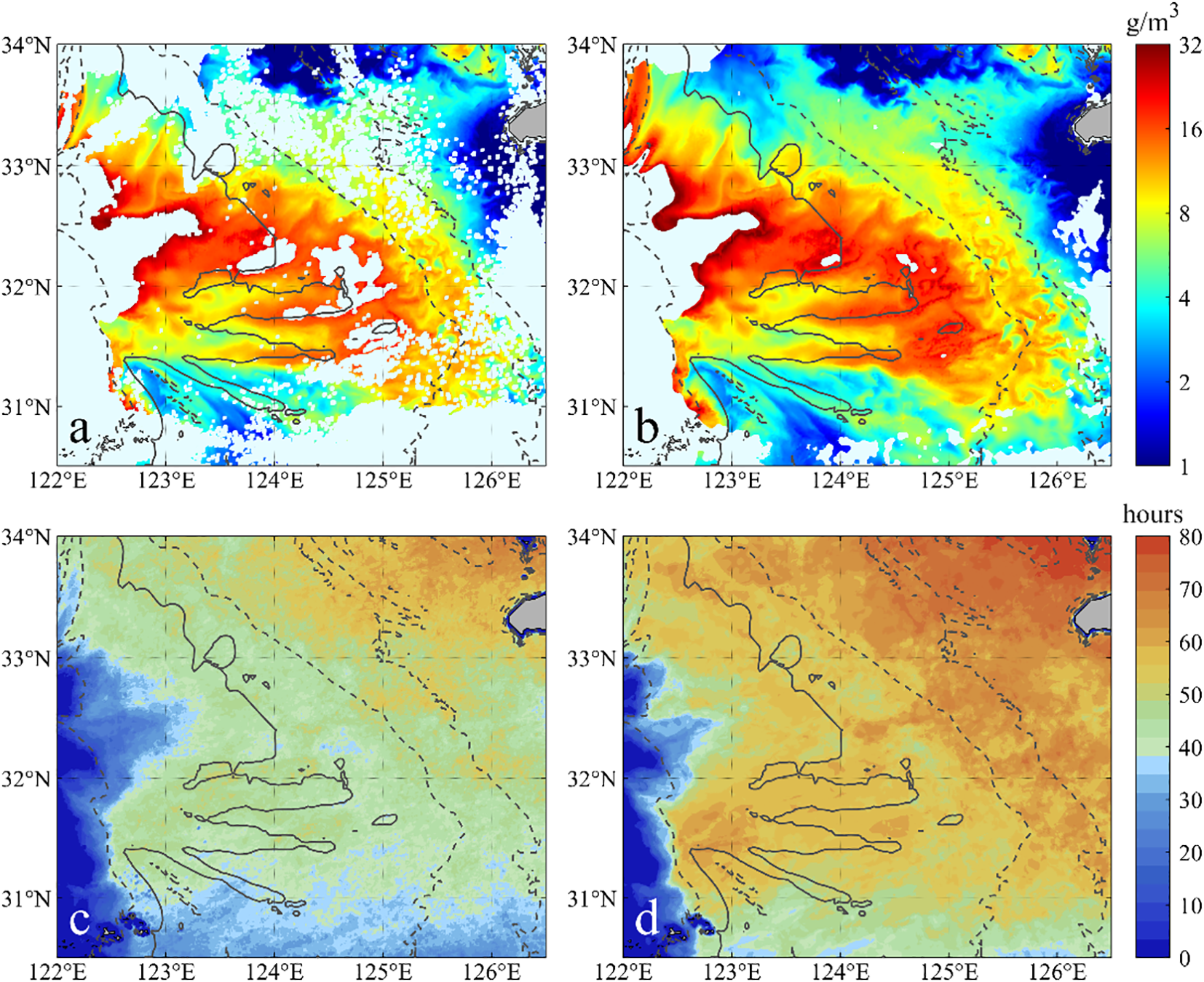
Figure 4. GOCI-TSS distribution at 11:16 on March 14, 2020: (a) before ST-Kriging; (b) after ST-Kriging. Cumulative amount of valid GOCI-TSS data during 08:16–15:16 from March 11 to 25, 2020: (c) before ST-Kriging; (d) after ST-Kriging.

2.2.2 Calculation of TSS daily range and daily mean

To better utilize the eight hourly GOCI-TSS observations for quantitatively analyzing the spring-neap evolution of TSS, this study proposes the following methods for deriving the daily range (ΔTSS) and daily mean (TSS_daily) of TSS. Taking Area A on March 20, 2020, as an example (Figure 5), the process is explained as follows.

Figure 5

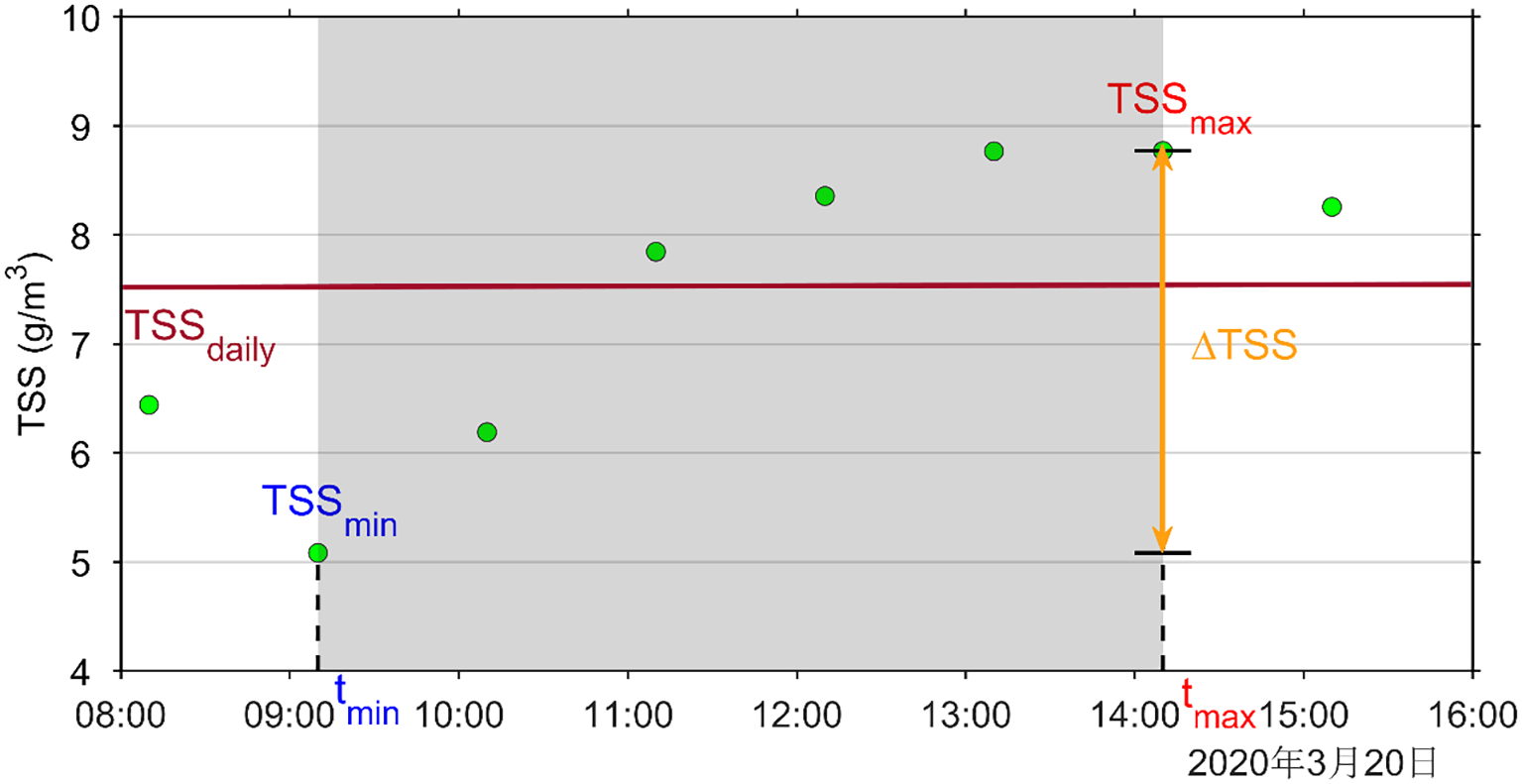
Figure 5. Schematic diagram of the calculation of TSS_daily and ΔTSS. The green dots represent the hourly GOCI sampling points, and the shaded areas indicate the calculation intervals for TSS_daily and ΔTSS.

2.2.2.1 ΔTSS

Defined as the difference between the maximum (TSS_max) and minimum (TSS_min) TSS concentrations within GOCI’s 8-hour observations window. This metric roughly quantifies the amplitude of diurnal TSS variations, expressed as Equation 1:

$\begin{array}{ll}\Delta TSS=TS{S}_{max}-TS{S}_{min}& (1)\end{array}$

2.2.2.2 TSS_daily

Due to tidal asymmetry, quarter-diurnal TSS variation exhibits significant diurnal differences in intensity. Moreover, the 8-hour GOCI observation window surpasses the 6.2-hour TSS quarter-diurnal cycle, making a simple 8-hour arithmetic mean inadequate for accurately representing the daily average level of TSS. Therefore, TSS_daily is defined as the arithmetic mean of all valid observations within the period of strongest concentration fluctuation [t_min, t_max], expressed as Equation 2:

$\begin{array}{ll}TS{S}_{daily}=\frac{1}{n}{\displaystyle \sum _{i=1}^{n}TS{S}_i,i=1,\dots ,n}& (2)\end{array}$

where n denotes the number of valid observations within the above period, and TSS_i represents the TSS concentration at the i-th time point.

By focusing on the period of strongest TSS fluctuation captured by GOCI, this method helps mitigate statistical biases caused by insufficient sampling duration and the asymmetry in the intensity of quarter-diurnal TSS variations, thereby providing more reliable results for analyzing spring-neap variations in TSS.

2.2.3 Calculation of TSS advection-diffusion equation and tidal mixing parameter

To explore the dynamic mechanism underlying TSS spring-neap variations, this study derives the TSS advection-diffusion equation (Simpson and Sharples, 2012) based on hourly GOCI-TSS data and FVCOM-derived tidal currents, as follows:

$\begin{array}{ll}\frac{\partial S}{\partial t}=V·\nabla S-\nabla ·G+\sum & (3)\end{array}$

where S. denotes TSS concentration; $V$ is the horizontal tidal current vector (with $u$ and $v$ representing the zonal and meridional tidal current components, respectively); $G=(\overline{u^{\prime }{S}^{\prime }},\overline{v^{\prime }{S}^{\prime }})$ is the horizontal diffusion flux; $u^{\prime }$, $v^{\prime }$, $S^{\prime }$ represent anomalies of u, v, S. On the left side of Equation 3, $\frac{\partial S}{\partial t}$ represents the local change term of TSS (denoted as CHA); on the right side, $V·\nabla S$ represents the horizontal advection term (denoted as ADV); $-\nabla ·G$ represents the horizontal diffusion term (denoted as DIF); and $\sum$ represents all other terms related to vertical processes—including the convection, diffusion, and settling of TSS in vertical (denoted as VER). Due to the lack of profile data, VER is calculated as the residual of CHA minus ADV and DIF.

Existing studies have shown that vertical convection and diffusion of TSS in macrotidal seas are primarily driven by tidal mixing (Shi and Wang, 2010; Luo et al., 2017; Zhou et al., 2020a). To quantitatively evaluate tidal mixing intensity, this study adopts the tidal mixing parameter ($SH$) proposed by Simpson and Hunter (1974), calculated as follows:

$\begin{array}{ll}SH=lo{g}_{10}(\frac{H}{U^3})& (4)\end{array}$

where $U=\sqrt{u^2+v^2}$ is the magnitude of tidal current velocity; H is the water depth below mean sea level. Notably, SH exhibits an inverse relationship with vertical mixing intensity, lower SH values indicate stronger tidal mixing, and has been widely applied in studies of short-term variations in tidal mixing intensity (Du et al., 2021; Ni et al., 2016; Zhou et al., 2020a).

3 Results

3.1 Spatial pattern and spring-neap variation of TSS

3.1.1 Spatial pattern of TSS

Using hourly GOCI-TSS data from March 11 to 25, 2020 (with no valid data on March 13 and 22), this study calculated the average values ($\overline{TS{S}_{daily}}$, $\overline{\Delta TSS}$; Figures 6a, c) and standard deviations (${\sigma }_{TS{S}_{daily}}$, ${\sigma }_{\Delta TSS}$; Figures 6b, d) of TSS_daily and ΔTSS over the spring-neap cycle, to analyze the spatial patterns of their average intensity and fluctuation magnitudes during this period.

Figure 6

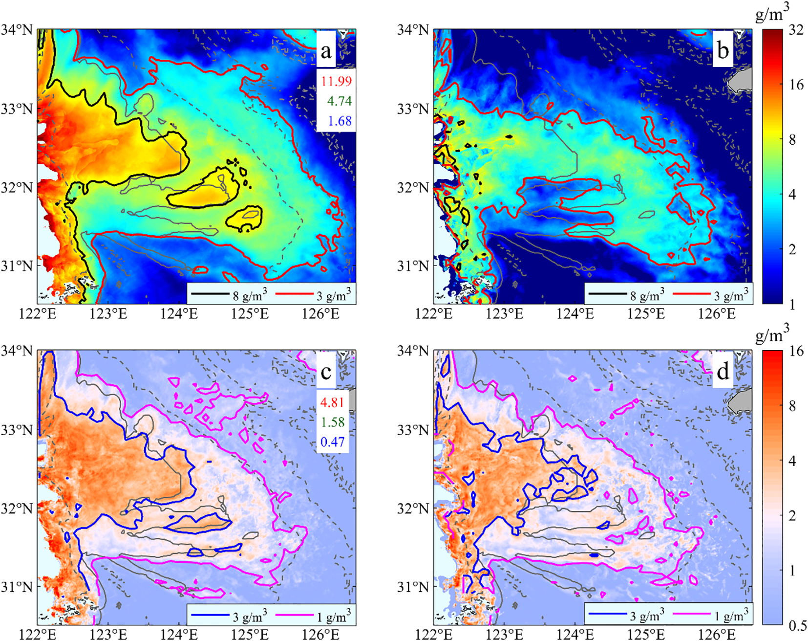
Figure 6. (a, b) show the distribution of the average value and standard deviation of TSS_daily (i.e., $\overline{TS{S}_{daily}}$ and ${\sigma }_{TS{S}_{daily}}$) during the spring-neap cycle, respectively; (c, d) show the distribution of the average value and standard deviation of ΔTSS (i.e., $\overline{\Delta TSS}$ and ${\sigma }_{\Delta TSS}$) during the spring-neap cycle, respectively. In (a) and (c), the red, green, and blue numbers represent the regional averages of $\overline{TS{S}_{daily}}$ and $\overline{\Delta TSS}$ in the H-, M- and L-Zones, respectively (unit: g/m³).

For the spatial patterns of $\overline{TS{S}_{daily}}$ and $\overline{\Delta TSS}$ (Figures 6a, c), the spatial distributions of the two show a significant positive correlation, generally decreasing progressively with increasing water depth, forming a tongue-shaped pattern extending from the Subei Shoal southeastward into open sea. Based on the 8 g/m³ and 3 g/m³ contours of $\overline{TS{S}_{daily}}$, this pattern can be roughly divided into high-, medium-, and low-turbidity & diurnal-variability zones (referred to as H-Zone, M-Zone, and L-Zone, respectively). Specifically, the H-Zone is distributed in nearshore and submarine sand dune areas at depths shallower than 40 m. Here, both $\overline{TS{S}_{daily}}$ and $\overline{\Delta TSS}$ within H-Zone decrease southeastward, displaying a stepped pattern along three latitudinally oriented dunes near 32.4°N, 31.8°N, and 31.6°N. The regional averages of $\overline{TS{S}_{daily}}$ and $\overline{\Delta TSS}$ in H-Zone are approximately 12.0 g/m³ and 4.8 g/m³, respectively. The M-Zone is distributed in areas of moderate depth on the Changjiang Bank, with regional averages of about 4.7 g/m³ for $\overline{TS{S}_{daily}}$ and 1.6 g/m³ for $\overline{\Delta TSS}$, while the L-Zone in offshore deeper waters has regional averages of about 1.7 g/m³ for $\overline{TS{S}_{daily}}$ and 0.5 g/m³ for $\overline{\Delta TSS}$.

For the spatial patterns of ${\sigma }_{TS{S}_{daily}}$ and ${\sigma }_{\Delta TSS}$ (Figures 6b, d), their spatial patterns largely consistent with their respective average values, also decreasing progressively with increasing water depth. In the H-Zone, the regional average TSS_daily ranges from 6.7 to 19.5 g/m³, while $\Delta TSS$ ranges from 1.0 to 10.5 g/m³. In the M-Zone, the regional average TSS_daily ranges from 2.0 to 9.6 g/m³, and ΔTSS ranges from 0.2 to 4.2 g/m³. In the L-Zone, the regional average TSS_daily ranges from 0.9 to 3.0 g/m³, and ΔTSS ranges from 0.1 to 1.3 g/m³. These results indicate that both TSS_daily and ΔTSS exhibit significant temporal variability over the spring-neap cycle, and the magnitude of this variability is positively correlated with their average intensities. The spring-neap fluctuations are most pronounced in the H-Zone.

In summary, the spatial patterns of both the average intensities and fluctuation magnitudes of TSS_daily and ΔTSS during the spring-neap cycle are regulated by seabed topography. The nearshore and submarine sand dune areas at depths shallower than 40 m (the H-Zone), characterized by high TSS concentrations, large daily ranges, and intense spring-neap fluctuations, are thus identified as key regions for subsequent analysis of TSS dynamics over a spring-neap cycle.

3.1.2 Spring-neap variations of TSS

Compared to their average spatial patterns, the daily distributions of TSS_daily and ΔTSS from March 11 to 25, 2020 (Figure 7, 8, 9, 10) exhibit pronounced spring-neap variations, with the H-Zone showing the most pronounced response. This paper describes the spatiotemporal evolution of TSS by integrating the following aspects: (1) changes in the distribution patterns and intensities of TSS_daily and ΔTSS, where the morphological features are represented by contour outlines, and the intensities are quantified by calculating the regional averages of TSS_daily and ΔTSS within the three sub-regions defined in Figure 6a; (2) verification of the consistency of the TSS temporal evolution by combining it with the TSS time-series from representative Area A within the H-Zone.

Figure 7

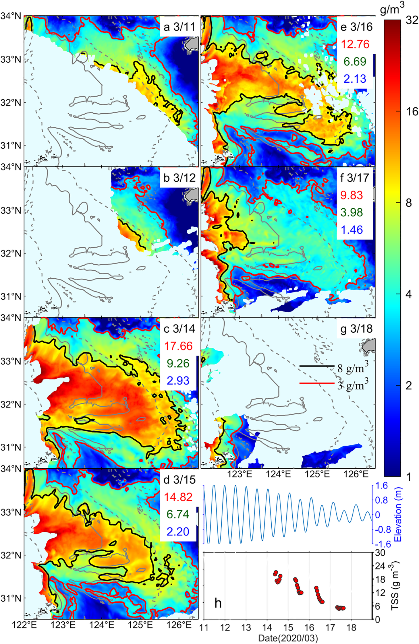
Figure 7. From spring to neap tide, March 11–18, 2020: GOCI-derived TSS_daily over the Changjiang Bank, the red, green, and blue numbers represent the regional averages of TSS_daily in the H-, M-, and L-Zones, respectively (unit: g/m³); the thick black and red lines denote the isolines where TSS_daily equals 8 g/m³ and 3 g/m³, respectively (a–g); variations of tidal elevation and TSS concentration in Area A (h).

Figure 8

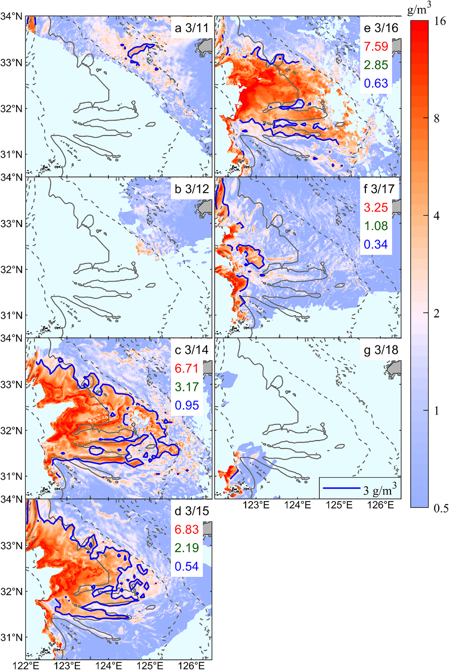
Figure 8. GOCI-derived ΔTSS over the Changjiang Bank from spring to neap tide, March 11–18, 2020. The red, green, and blue numbers represent the regional averages of ΔTSS in the H-, M-, and L-Zones, respectively (unit: g/m³); the thick blue line denotes the isoline where ΔTSS=3 g/m³ (a–g).

Figure 9

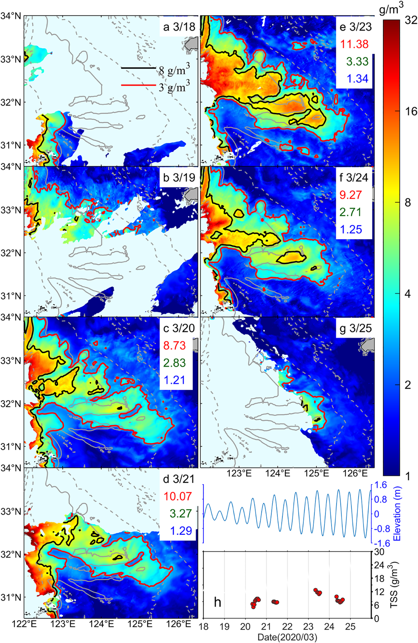
Figure 9. From neap to spring tide, March 18–25, 2020: GOCI-derived TSS_daily over the Changjiang Bank, the red, green, and blue numbers represent the regional averages of TSS_daily in the H-, M-, and L-Zones, respectively (unit: g/m³); the thick black and red lines denote the isolines where TSS_daily equals 8 g/m³ and 3 g/m³, respectively (a–g); variations of tidal elevation and TSS concentration in Area A (h).

Figure 10

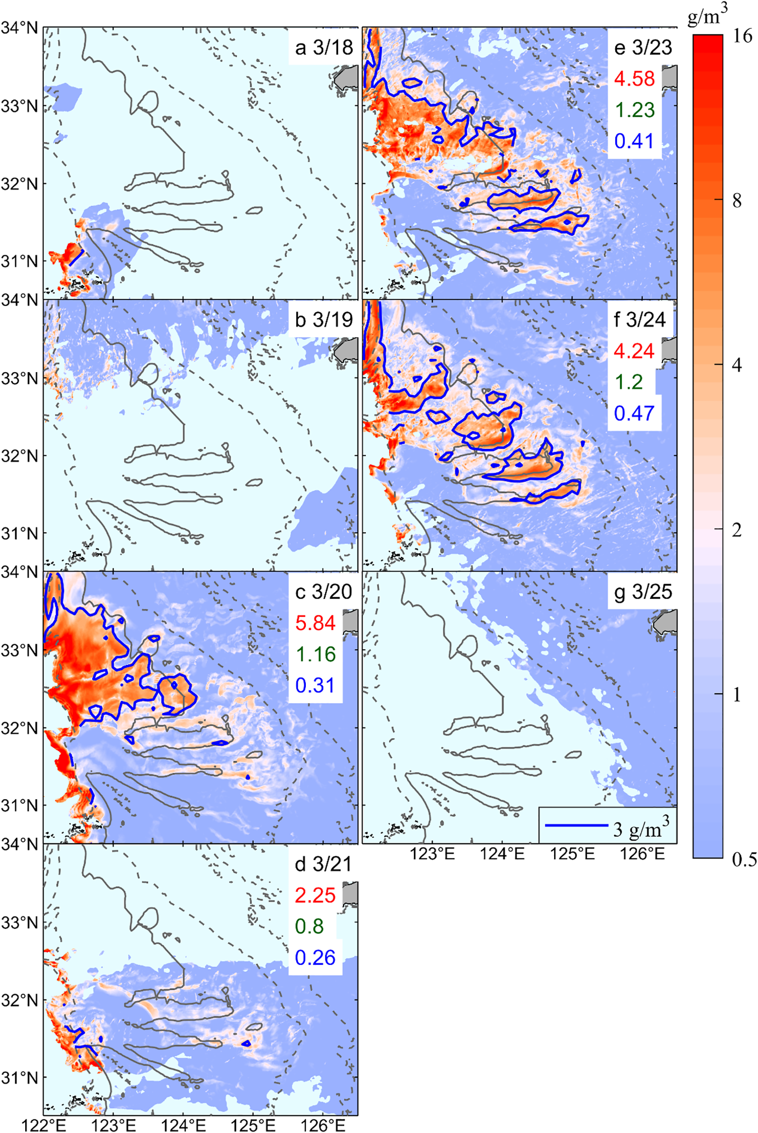
Figure 10. GOCI-derived ΔTSS over the Changjiang Bank from neap to spring tide, March 18–25, 2020. The red, green, and blue numbers represent the regional averages of ΔTSS in the H-, M-, and L-Zones, respectively (unit: g/m³); the thick blue line denotes the isoline where ΔTSS=3 g/m³ (a–g).

Given that the observation period fully encompasses an entire “spring-neap-spring” tidal cycle, it is divided into two phases based on tidal current intensity: March 11–18 as the spring-to-neap transition phase, and March 18–25 as the neap-to-spring transition phase. It should be noted that despite interpolation, the data still struggle to achieve full 8-hour coverage for each day (see Supplementary Figures S1, S2), and the statistics (particularly ΔTSS) for regions with severe data gaps may have significant biases. Therefore, in the specific analysis, March 13 and 22 are excluded due to a lack of valid data; and regional statistics were not performed for March 11–12, 18–19, and 25 due to excessively low spatial coverage of the TSS imagery. The detailed description of the TSS evolution for the two phases is provided below.

(1) Spring-to-neap transition phase (March 11–18, Figures 7, 8).

The general characteristics of this phase were as follows: except for a brief increase in TSS_daily during the early middle tide period, both TSS_daily and ΔTSS over the Changjiang Bank decreased substantially, by approximately 50% and 60%, respectively, as tidal intensity weakened. Spatially, the most pronounced changes occurred in the H-Zone, which evolved from an extensive, continuous NW-SE oriented distribution into a narrow, band-like structure before largely dissipating by the neap tide. The previously observed stepped pattern disappeared, while the M-Zone also retreated shoreward.

The detailed evolution process is as follows: Partial imagery from March 11 showed that the H- and M-Zones extended to depths greater than 60 m and 80 m, respectively. Subsequently, they contracted toward shallower areas, by March 12, their boundaries had retreated to the vicinity of the 60-m and 80-m isobaths (Figures 7a, b), indicating the onset of a decline in TSS_daily. A synchronous weakening of ΔTSS was also observed (Figures 8a, b). Observations from March 14 to 17 were continuous and relatively complete (Figures 7c–f, 8c–f). On March 14, the H-Zone exhibited an extensive, continuous NW-SE oriented distribution, with a spatial extent even exceeding that observed during the spring tide on the 11th, reaching the 80-m isobath. This spatial pattern differed notably from the separate, stepped pattern observed under average conditions (Figure 6a). Thereafter, the H-Zone contracted rapidly, transforming into a narrow NW-SE band-like distribution, while the M-Zone also experienced slight shoreward contraction. By March 17, during the neap tide, the H-Zone had largely dissipated across most of the area, persisting only nearshore. The M-Zone also contracted substantially, with its edges appearing as fragmented patches. Local imagery from March 18 indicated further shoreward retreat of both the H- and M-Zones, with TSS_daily and ΔTSS dropping to their lowest levels during the observation period (Figure 7g, 8g).

In terms of intensity, the regional averages of TSS_daily across the H-, M-, and L-Zones decreased by approximately 50%. ΔTSS also exhibited a fluctuating decline in response to the reduction in background concentration, with an average decline of about 60%. The TSS evolution in Area A (Figure 7h) was consistent with the overall trend observed in the H-Zone, with TSS_daily and ΔTSS decreasing by 73% and 86%, respectively, further confirming the high responsiveness of H-Zone to tidal variation.

(2) Neap-to-spring transition phase (March 18–25, Figures 9, 10).

The general characteristics of this phase were as follows: Both TSS_daily and ΔTSS showed a fluctuating upward trend with increasing tidal forcing, though their average intensities were generally lower than during the spring-to-neap transition, and a significant decline was observed by the end of the phase. Spatially, the H-Zone progressively developed and expanded southeastward from the nearshore along submarine dunes within the 40-m isobath, reestablishing the previously identified stepped pattern. The M-Zone also extended seaward synchronously. However, by the late phase, the spatial extent of the H-Zone had contracted noticeably.

The detailed evolution process is as follows: Partial nearshore imagery indicated clear seaward expansion of both the H- and M-Zones (Figures 9a–b, 10a–b), marking the onset of increases in TSS_daily and ΔTSS. Observations from March 20 to 23 were relatively continuous and complete (Figures 9c–f, 10c–f). On March 20, the H-Zone began to form in the northwestern dune field, though its distribution remained discontinuous. The M-Zone exhibited a stepped pattern along the edges of the three submarine dunes, with strong diurnal variation primarily observed in the northwestern dune region. The H-Zone then progressively extended southeastward, reaching its maximum spatial extent for this phase by March 23 and forming a partially connected stepped pattern. The M-Zone expanded synchronously and reached its maximum outline on the same day. By this time, TSS_daily and ΔTSS had generally peaked. Additionally, a low-turbidity tongue in the southwestern submarine canyon area continued to extend northward, with its coverage expanding progressively. By the end of the phase (March 24–25), despite a slight increase in tidal forcing, the H-Zone contracted markedly, displaying a separated stepped pattern.

In terms of intensity, from March 18 to 23, TSS_daily and ΔTSS increased across all zones, except for an approximately 17% decrease in ΔTSS within the H-Zone. In the late phase (March 24), a significant reversal occurred: TSS_daily in the H- and M-Zones decreased markedly by about 19%, accompanied by a slight corresponding decrease in ΔTSS. The TSS variation in Area A (Figure 9h) showed that its TSS_daily followed a consistent “increase-then-decrease” trend similar to that in H-Zone, whereas its ΔTSS exhibited a “decrease-then-increase” trend, diverging from the H-Zone.

In summary, the increase in TSS_daily during the early stage of this phase largely corresponded to enhanced tidal forcing. However, the widespread decline in intensity by the late phase suggests that, in addition to tidal dynamics, other factors may have jointly regulated the spatiotemporal evolution of TSS. Furthermore, the asynchronous variation between ΔTSS and background TSS concentration may also be related to insufficient effective GOCI observations in localized areas during this phase (Supplementary Figure S2).

3.2 Dynamic mechanism

3.2.1 Tide-induced mixing

Observations over a 15-day period show that the variations of TSS_daily and ΔTSS over the Changjiang Bank generally follows the spring-neap cycle. To explore the underlying mechanisms, this study integrates hourly GOCI-TSS data with concurrent tidal current simulations from FVCOM. By quantitatively solving the TSS advection-diffusion equation (Equation 3) during spring, middle, and neap tidal phases, the contributions of the horizontal advection term (ADV), horizontal diffusion term (DIF), and vertical related term (VER) to the local changes in TSS (CHA) were evaluated. To ensure comparability across different tidal phases, the analysis time intervals were uniformly selected as the GOCI observation slots adjacent to the time when the tidal elevation in Area A approached 0 m. Specifically, these intervals included the neap tide period (March 17, 13:16–14:16), the mid-tide period (March 20, 11:16–12:16), and the spring tide period (March 24, 13:16–14:16). The following analysis, in conjunction with the spatial distribution characteristics of each term in Equation 3 and their temporal variations in Area A (Figure 11), explores the dominant dynamic factors governing the spatiotemporal variations of TSS.

Figure 11

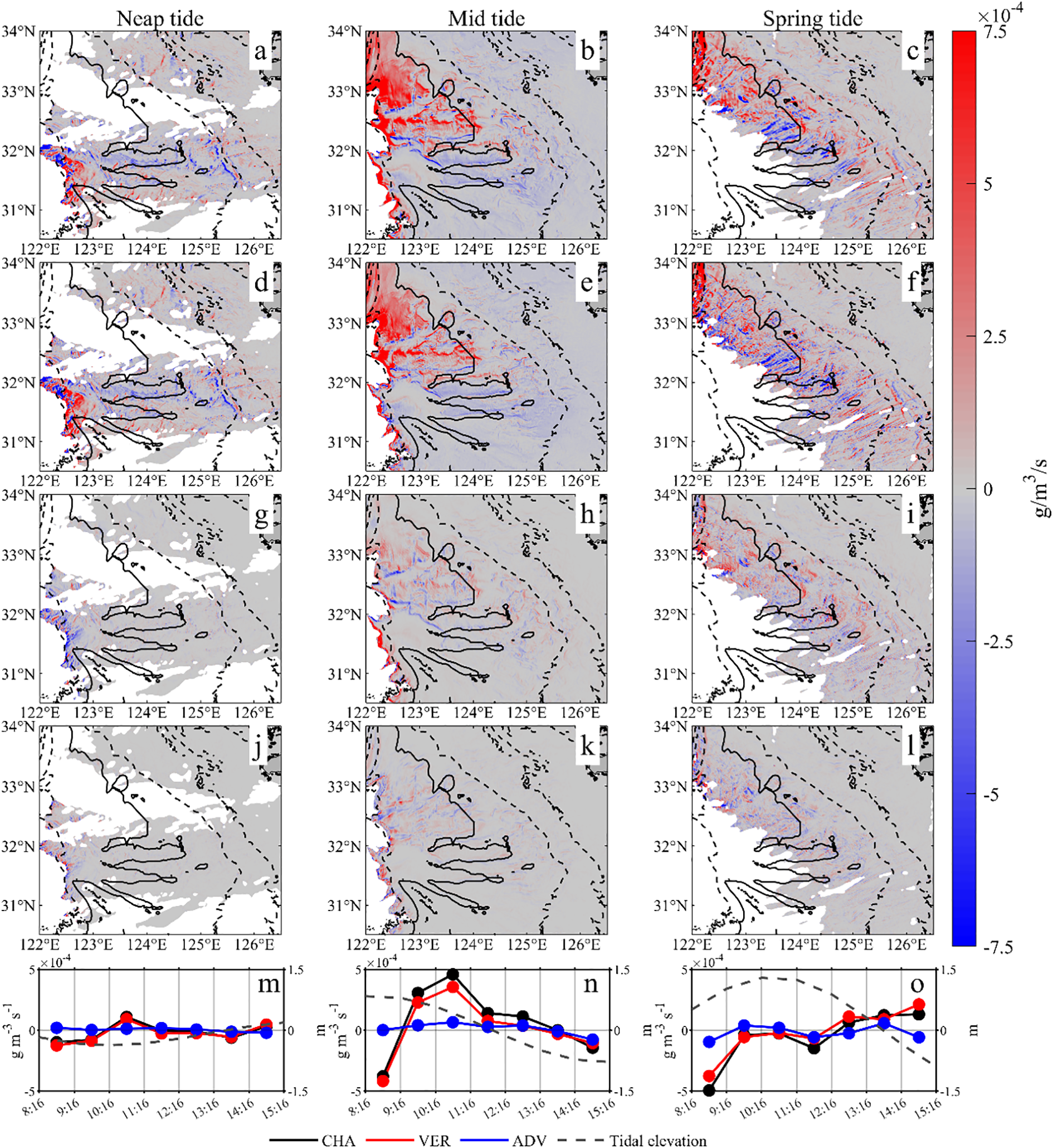
Figure 11. The spatial distribution of CHA (a–c), VER (d–f), ADV (g–i), and DIF (j–l) during neap tide (March 17, 13:16–14:16), mid-tide (March 20, 11:16–12:16), and spring tide (March 24, 13:16–14:16), respectively, as well as the hourly variations of each term in Area A (m–o).

From the spatial distribution characteristics, during different tidal phases, the absolute values of CHA (Figures 11a–c) are larger in coastal and sand dune areas at depths shallower than 40 m and gradually decrease with increasing depth. The average order of magnitude of CHA reaches O (10–⁴ g/m³/s). Further analysis of the contributions of each dynamic term shows that ADV is only significant in localized regions strong horizontal TSS gradients, such as the coastal strong frontal zone and the boundaries between H-, M- and L-zones (Figures 11g–i), with an average order of magnitude of only O (10–⁵ g/m³/s), indicating a limited contribution to CHA. The values of DIF (Figures 11j–l) are even lower, also averaging O (10–⁵ g/m³/s). Evidently, the influences of ADV and DIF on CHA within the study area are minor, representing secondary factors. In contrast, the spatial distribution of VER (Figures 11d–f) highly coincides with that of CHA, with an average magnitude reaching O (10^-4 g/m³/s), consistent with the magnitude of CHA. From the temporal evolution, based on the hourly variations of each term (excluding DIF, which has the smallest contribution) in area A during different tidal phases (Figures 11m–o), it is observed that within each tidal phase, CHA and VER remain highly synchronized and of comparable magnitude, with an average correlation coefficient as high as 98%. Conversely, the magnitude of ADV is significantly lower than that of CHA, and their temporal synchronization is poor, indicating that ADV also acts as a secondary factor influencing the temporal variations of CHA. By synthesizing the spatial distribution and temporal variation of each term in Equation 3, it can be inferred that the spatiotemporal variations of TSS over the Changjiang Bank during the spring-neap cycle are predominantly controlled by VER, which encompasses vertical processes such as convection, diffusion, and settling of TSS.

Existing studies have shown that the tidal rhythmic variations of TSS in macrotidal regions are primarily modulated by vertical tidal mixing (Luo et al., 2017; Zhou et al., 2020a; Du et al., 2021). Considering this, we employed the tidal mixing parameter SH (Equation 4) to quantify the tidal mixing intensity, and explored the influence of tidal mixing on the spatiotemporal variations of TSS_daily and ΔTSS over the Changjiang Bank by analyzing the averaged spatial distribution and daily dynamical variations of SH over the spring-neap cycle.

To elucidate the regulatory mechanism of tidal mixing on the spatial patterns of TSS, this study conducted analyses from two perspectives: (1) the spatial pattern of $\overline{SH}$ (tidal mixing intensity averaged over the spring-neap cycle); and (2) the correlations between $\overline{SH}$ and both the averaged TSS daily mean ($\overline{TS{S}_{daily}}$) and daily range ($\overline{\Delta TSS}$). As shown in the spatial distribution of $\overline{SH}$ (Figure 12a), tidal mixing intensity generally decreases exponentially with increasing water depth, forming a northwest-southeast oriented tongue-shaped distribution. Notably, the $\overline{SH}$=2.4 and $\overline{SH}$=2.6 isopleths align closely with the boundaries of the three subregions (H-, M- and L-Zones), allowing the study area to be classified into strong-, moderate-, and weak-mixing zones. This spatial configuration corresponds strongly with the distributions of $\overline{TS{S}_{daily}}$ and $\overline{\Delta TSS}$. Correlation analysis in the double-logarithmic coordinate system (Figures 12b, c) further reveals that $\overline{SH}$ is significantly linearly correlated with both ${\text{log}}_{10}(\overline{TS{S}_{daily}})$ and ${\text{log}}_{10}(\overline{\Delta TSS})$, with R² reaching 0.77 and 0.79, respectively. This indicates that regions with stronger tidal mixing are associated with higher values of both TSS_daily and ΔTSS. Integrating the spatial patterns and correlation results, it can be concluded that the spatial distribution of tidal mixing intensity, modulated by water depth, serves as the dominant dynamic factor governing the spatial patterns of TSS_daily and ΔTSS over the Changjiang Bank.

Figure 12

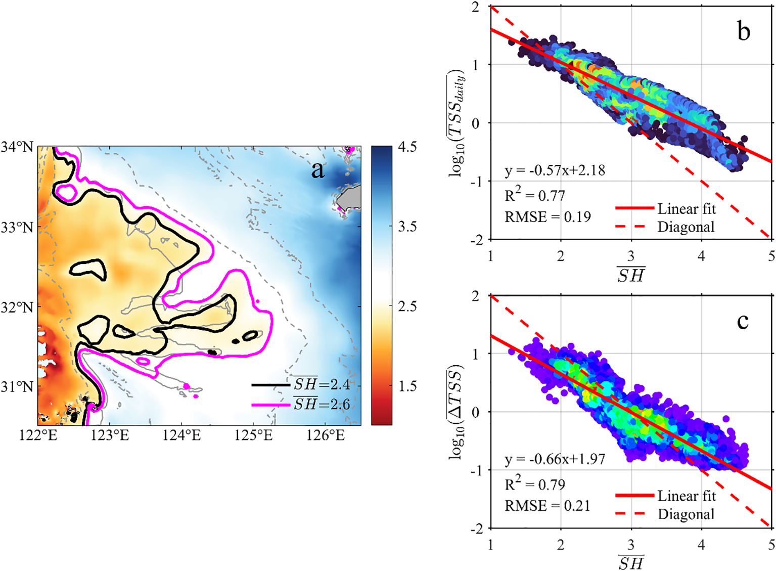
Figure 12. (a) Distribution of the average tidal mixing intensity ($\overline{SH}$) during the observation period; (b) scatters of ${\text{log}}_{10}(\overline{TS{S}_{daily}})$ and $\overline{SH}$ along with their linear fitting; (c) scatters of ${\text{log}}_{10}(\overline{\Delta TSS})$ and $\overline{SH}$ along with their linear fitting.

Furthermore, the tidal mixing intensity also exhibits spring-neap fluctuations as tidal current velocity varies, which is likely the dominant factor driving the spring-neap variations of TSS_daily and ΔTSS. Considering that TSS_daily derived from GOCI data is more accurate than ΔTSS, TSS_daily was used as the representative indicator to analyze its temporal correlation with tidal mixing intensity. During the spring-neap cycle, the variation of TSS_daily is most significant in the H-Zone; additionally, the morphologies of the $\overline{SH}$=2.4 and $\overline{TS{S}_{daily}}$=8 g/m³ isolines are highly consistent with that of the H-Zone. Therefore, this study plotted the daily distribution of the SH = 2.4 isoline (referred to as SH_2.4​) and TSS_daily=8 g/m³ isoline (referred to as TSS_{daily_8}) over the spring-neap cycle (Figure 13). These isolines respectively indicate the daily tidal mixing intensity and TSS concentration in the H-Zone. By tracking the dynamic changes in their morphology and position, the impact of spring-neap fluctuations in tidal mixing intensity on the daily evolution of TSS_daily was revealed.

Figure 13

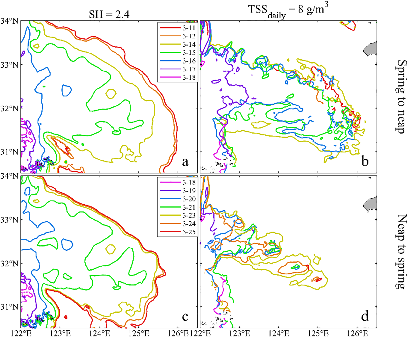
Figure 13. Distribution of isolines for SH = 2.4 and TSS_daily=8 g/m³: (a, b) spring-to-neap transition phase; (c, d) neap-to-spring transition phase.

Although there were differences in the morphology and position between SH_2.4 and TSS_{daily_8}, their variation trends were highly consistent, which was specifically reflected in the following two-stage characteristics:

1. Spring-to-neap transition period (March 11–18) (Figures 13a, b). During this stage, SH_2.4 continuously contracted shoreward as tidal current weakened, showing a stage-specific characteristic of “slight shoreward movement during spring tide, significant shoreward leap during mid-tide, and retreat to the coast with almost disappearance during neap tide”. This indicated that tidal mixing intensity slightly attenuated during spring tide, dropped rapidly during middle tide, and entered a weak mixing state during neap tide. Meanwhile, except for an abnormal expansion on the 14th, TSS_{daily_8} generally showed a consistent variation trend with SH_2.4, confirming that TSS_daily decreased synchronously with the weakening of tidal mixing intensity.

2. Neap-to-spring transition period (March 18–25) (Figures 13c, d). Contrary to the previous stage, SH_2.4 continuously expanded seaward as tidal currents intensified. Specifically, from neap to mid-tide (18th–23rd), SH_2.4 moved rapidly seaward by over three longitudes, indicating a rapid increase in tidal mixing intensity. Correspondingly, TSS_{daily_8} expanded synchronously, indicated TSS_daily rose steadily and reached its stage peak on the 23rd. Upon entering spring tide (24th–25th), despite the continuous slight expansion of SH_2.4​ and a minor increase in tidal mixing intensity, TSS_{daily_8} contracted abnormally and TSS_daily decreased accordingly. This suggested that other factors may be involved in the joint regulation of TSS during this period, causing TSS_daily variation to deviate from the spring-neap tidal regularity, which required further investigation.

In summary, the temporal fluctuations of tidal mixing intensity induced by tidal current velocity are the dominant dynamic factors that drive the spring-neap evolution of TSS_daily and ΔTSS.

3.2.2 Seawater stratification

Although tidal mixing is the dominant dynamic factor of spring-neap TSS variations, the variation of TSS_daily and ΔTSS over extensive areas during certain periods (e.g., March 14 and 24–25, 2020) cannot be fully explained by tidal mixing alone, implying the existence of other regulatory factors. Given that the seasonal variation amplitude of TSS on the YECS is much larger than that of the spring-neap and quarter-diurnal scales (Shi and Wang, 2010; Luo et al., 2017; Zhou et al., 2017, 2020b), this study focused on the winter high-TSS period to eliminate the interference of seasonal variations, and assumed that the water temperature over the Changjiang Bank was relatively stable during the observation. However, the observation period coincides with the winter-to-spring transition, during which sea surface temperature (SST) showed a steady upward trend due to increasing solar radiation, as well as significant short-term fluctuations caused by alternating cold and warm air masses.

As shown in the daily SST from Himawari-8 (Figure 14), SST fluctuated upward during the observation, with a cumulative SST increase of 4.1°C in waters shallower than 40 m. Notably, a rapid drop in regional average SST by nearly 1°C on March 13 was followed by a significant rise in TSS_daily the next day. After March 20, the southern Changjiang Bank (south of 32°N) was progressively covered by extensive warm water. In particular, the regional average SST surged by 1.6°C from March 23 to 25, accounting for 39% of total SST increase. This coincided with the decline of TSS_daily in the final stage of the observation.

Figure 14

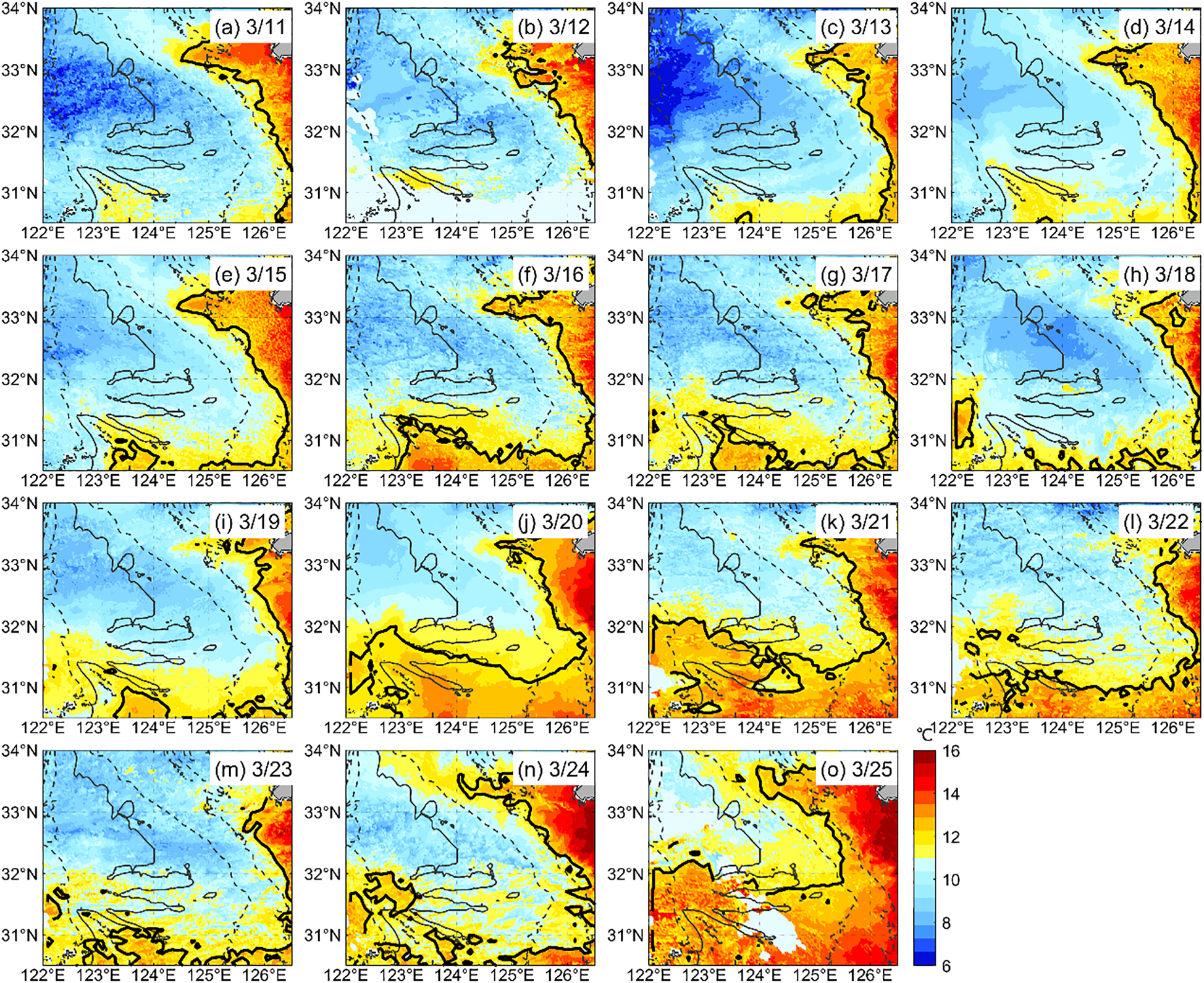
Figure 14. Daily SST distribution over the Changjiang Bank based on Himawari-8, with the thick black line indicating the 12 °C isotherm.

To explore the underlying mechanism, we used the buoyancy frequency (N²) to represent the strength of water stratification and the Froude number (Fr^-¹) to indicate the relative importance of tidal forcing versus stratification at different water depths (see Supplementary Materials for calculation methods). Further analysis of the regional averages of SST, N², and Fr^-¹ over the Changjiang Bank (Figure 15) showed that N² largely followed the variations in SST, while Fr^-¹ exhibited a spring-neap cyclic pattern generally consistent with tidal intensity. However, during March 23–25, despite continued strengthening of tidal currents, Fr^-¹ decreased markedly due to a sharp increase in N², suggesting that enhanced stratification likely suppressed tidal mixing.

Figure 15

Figure 15. Variations of regional averages of SST, N², and Fr^-1 over the Changjiang Bank from March 11 to 25, 2020.

It can thus be inferred that the abrupt SST rise at the end of the observation period likely promoted the formation of a pycnocline, which hindered the diffusion of bottom sediments to the surface and ultimately caused a decrease in surface TSS during spring tide. However, due to the lack of synchronous temperature-salinity (T-S) profiles, the calculations of N² and Fr^-¹ involve uncertainties. Therefore, the analysis in this study primarily references their variation trends, and it is not yet possible to precisely quantify the stratification intensity and the degree of its inhibition on tidal mixing.

4 Conclusions and discussions

Based on hourly GOCI-TSS data from March 11 to 25, 2020, this study applied ST-Kriging to reconstruct the hourly TSS dataset. This approach effectively mitigated the dual limitations of limited spatial coverage in field observations and insufficient temporal resolution of polar-orbiting satellites. Taking the winter Changjiang Bank as a representative case, this approach systematically revealed the spatiotemporal evolution of TSS_daily and ΔTSS over a complete spring-neap cycle.

The results show that both TSS_daily and ΔTSS over the Changjiang Bank exhibit a tongue-shaped distribution, decreasing from nearshore toward the southeastern offshore areas with increasing water depth. This pattern could be sequentially divided into high-, medium-, and low-turbidity & diurnal-variability zones (H-, M-, and L-Zones), consistent with previous studies (Luo et al., 2017; Zhou et al., 2020a, 2020b). More importantly, leveraging high-resolution GOCI imagery and measured bathymetric data, this study revealed for the first time a stepped pattern in the H-Zone along three latitudinal sand dunes near the 40-m isobath. The boundaries of H-Zone closely aligned with the moderate frontal activity area identified by Du et al. (2023), confirming the influence of geomorphology on TSS distribution.

Over the 15-day observation period, TSS_daily and ΔTSS exhibited evident spring-neap variability, particularly within the H-Zone. During spring-to-neap transition phase, TSS_daily and ΔTSS decreased significantly by approximately 50% and 60%, respectively. Concurrently, the H-Zone rapidly contracted from a broad, continuous NW–SE oriented distribution to a narrow band, losing its stepped pattern by neap tide. In contrast, during neap-to-spring transition phase, both TSS_daily and ΔTSS showed fluctuating increases, and the H-Zone gradually expanded southeastward, reestablishing its stepped pattern. However, by the end of this phase, TSS_daily and ΔTSS declined again, accompanied by a corresponding contraction of the H-Zone. These findings broaden the previously proposed simplistic pattern of “lower TSS during spring tide and higher TSS during neap tide” (Chen, 2001; Shi et al., 2011a; Zhou et al., 2020b), offering a detailed analysis of the complex spatiotemporal evolution of TSS over a spring-neap cycle. The results suggest that the actual variations may not strictly follow an idealized spring-neap periodicity.

Mechanism analysis suggests that tide-induced mixing, modulated by water depth and tidal currents velocity, dominates the spatiotemporal evolution of TSS_daily and ΔTSS, with water depth determining their spatial pattern and variations in tidal current velocity driving their spring-neap evolution. Furthermore, rapid increase in SST during the winter-spring transition may enhance water stratification, suppressing tidal mixing. This reasonably explains the observed deviation of TSS from the strengthening tidal trend at the end of the phase.

This study deepens the understanding of multi-scale TSS dynamics over the Changjiang Bank. The proposed analytical framework enables a more continuous and precise capture of TSS dynamics, achieving the first synchronous quantitative analysis of the spatiotemporal evolution of both TSS_daily and ΔTSS over a spring-neap cycle. These findings offer an empirical reference for designing multi-frequency TSS field surveys and setting time steps in numerical models.

Nevertheless, this study has limitations in interpreting TSS evolution and dynamic mechanism, due to GOCI’s observational constraints and the lack of concurrent T-S profiles. In terms of phenomenon interpretation, GOCI’s limited observation duration and cloud-induced data gaps may lead to discrepancies between observed and actual TSS variations—particularly the ΔTSS, which requires high data integrity. Future work could integrate multi-source satellite data, such as Himawari-8 (observation period: 06:00–18:00, temporal resolution: 10 min), GOCI-II (07:30–16:30, 1 h), and MODIS (1 d), to expand the observation window and improve the probability of obtaining valid data. For mechanism analysis, the lack of synchronous T-S profiles makes it difficult to quantify stratification intensity and its inhibitory effect on tidal mixing. In subsequent studies, satellite data can be used to optimize 3-D hydrodynamic-sediment coupling model to simulate sediment transport under different stratification conditions, thereby systematically clarifying the synergistic effect of tidal mixing and water stratification in TSS dynamics.

Data availability statement

The original contributions presented in the study are included in the article/Supplementary Material. Further inquiries can be directed to the corresponding author.

Author contributions

YZ: Conceptualization, Data curation, Formal analysis, Investigation, Methodology, Software, Supervision, Validation, Visualization, Writing – original draft, Writing – review & editing. JX: Resources, Supervision, Writing – review & editing, Validation. FZ: Funding acquisition, Resources, Supervision, Validation, Writing – review & editing, Project administration.

Funding

The author(s) declared that financial support was received for this work and/or its publication. The National Natural Science Foundation of China (Grant No. U23A2023, 42276021); The Key R&D Program of Zhejiang Province (Grant No. 2024C03034); The UN Ocean Decade Program “Kuroshio Edge Exchange and the Shelf Ecosystem” (No. CSK-2/08/2023). This work was supported by the high-performance computing cluster of State Key Laboratory of Satellite Ocean Environment Dynamics.

Acknowledgments

We are thankful for the Korea Ocean Satellite Center (KOSC) for providing the GOCI data (https://kosc.kiost.ac.kr/index.nm), the Qingdao Institute of Marine Geology, China Geological Survey, for providing the high-resolution bathymetric data, and the Japan Meteorological Agency (JMA) for providing the sea surface temperature data (Himawari-8) (https://www.eorc.jaxa.jp/ptree/).

Conflict of interest

The authors declare that the research was conducted in the absence of any commercial or financial relationships that could be construed as a potential conflict of interest.

Generative AI statement

The author(s) declare that no Generative AI was used in the creation of this manuscript.

Any alternative text (alt text) provided alongside figures in this article has been generated by Frontiers with the support of artificial intelligence and reasonable efforts have been made to ensure accuracy, including review by the authors wherever possible. If you identify any issues, please contact us.

Publisher’s note

All claims expressed in this article are solely those of the authors and do not necessarily represent those of their affiliated organizations, or those of the publisher, the editors and the reviewers. Any product that may be evaluated in this article, or claim that may be made by its manufacturer, is not guaranteed or endorsed by the publisher.

Supplementary material

The Supplementary Material for this article can be found online at: https://www.frontiersin.org/articles/10.3389/fmars.2025.1717752/full#supplementary-material

References

Bargaoui Z. K. and Chebbi A. (2009). Comparison of two kriging interpolation methods applied to spatiotemporal rainfall. J. Hydrol. 365, 56–73. doi: 10.1016/j.jhydrol.2008.11.025

Crossref Full Text | Google Scholar

Chen S. (2001). Seasonal, neap-spring variation of sediment concentration in the joint area between yangtze estuary and hangzhou bay. Sci. China Ser. B Chem. 44, 57–62. doi: 10.1007/BF02884809

Crossref Full Text | Google Scholar

Cho S. I., Ahn Y. H., Ryu J. H., Kang G. S., and Youn H. S. (2010). Development of geostationary ocean color imager (GOCI). Korean Journal of Remote Sensing. 26, 157–165. doi: 10.7780/kjrs.2010.26.2.239

Crossref Full Text | Google Scholar

Choi J., Park Y. J., Ahn J. H., Lim H., Eom J., and Ryu J. (2012). GOCI, the world’s first geostationary ocean color observation satellite, for the monitoring of temporal variability in coastal water turbidity. J. Geophys. Res.: Oceans 117, 2012JC008046. doi: 10.1029/2012JC008046

Crossref Full Text | Google Scholar

Du Y., Han X., Wang Y. P., Fan D., and Zhang J. (2025). Multiscale spatio-temporal variability of suspended sediment front in the Yangtze River estuary and its ecological effects. Water Res. 279, 123349. doi: 10.1016/j.watres.2025.123349

PubMed Abstract | Crossref Full Text | Google Scholar

Du Y., Lin H., He S., Wang D., Wang Y. P., and Zhang J. (2021). Tide-induced variability and mechanisms of surface suspended sediment in the zhoushan archipelago along the southeastern coast of China based on GOCI data. Remote Sens. 13, 929. doi: 10.3390/rs13050929

Crossref Full Text | Google Scholar

Du Y., Qin Y., Chu D., He S., Zhang J., Wang G., et al. (2023). Spatial and temporal variability of suspended sediment fronts over the Yangtze bank in the yellow and east China seas. Estuar. Coast. Shelf Sci. 288, 108361. doi: 10.1016/j.ecss.2023.108361

Crossref Full Text | Google Scholar

Emery W. J. and Thomson R. E. (2001). Data analysis methods in physical oceanography. 2nd Edn (Amsterdam New York: Elsevier).

Google Scholar

Fettweis M., Riethmüller R., Verney R., Becker M., Backers J., Baeye M., et al. (2019). Uncertainties associated with in situ high-frequency long-term observations of suspended particulate matter concentration using optical and acoustic sensors. Prog. Oceanogr. 178, 102162. doi: 10.1016/j.pocean.2019.102162

Crossref Full Text | Google Scholar

He X., Bai Y., Pan D., Huang N., Dong X., Chen J., et al. (2013). Using geostationary satellite ocean color data to map the diurnal dynamics of suspended particulate matter in coastal waters. Remote Sens. Environ. 133, 225–239. doi: 10.1016/j.rse.2013.01.023

Crossref Full Text | Google Scholar

Kilibarda M., Hengl T., Heuvelink G. B. M., Gräler B., Pebesma E., Perčec Tadić M., et al. (2014). Spatio-temporal interpolation of daily temperatures for global land areas at 1km resolution. J. Geophys. Res.: Atmos. 119, 2294–2313. doi: 10.1002/2013JD020803

Crossref Full Text | Google Scholar

Kong X., Lu K., Xu X., Yang H., Zhang Y., and Shang L. (2022). A study on the characteristic and its cause of topography and geomorphology of the south yellow sea. Mar. Geol. Quat. Geol. 42, 21–31. doi: 10.16562/j.cnki.0256-1492.2022072903

Crossref Full Text | Google Scholar

Li Y., Hu J., and Wu Z. (2021). Research on the variation of suspended sediment concentration in the bohai sea during the spring-neap tidal cycle based on GOCI images. Mar. Sci. Bull. 40, 348–360. doi: 10.11840/j.issn.1001-6392.2021.03.012

Crossref Full Text | Google Scholar

Lie H., Lee S., and Cho C. (2002). Computation methods of major tidal currents from satellite-tracked drifter positions, with application to the yellow and east China seas. J. Geophys. Res.: Oceans. 107, 3–1–3–22. doi: 10.1029/2001JC000898

Crossref Full Text | Google Scholar

Lin H., Yu Q., Wang Y., and Gao S. (2022). Assessment of the potential for quantifying multi-period suspended sediment concentration variations using satellites with different temporal resolution. Sci. Total Environ. 853, 158463. doi: 10.1016/j.scitotenv.2022.158463

PubMed Abstract | Crossref Full Text | Google Scholar

Lophaven S. N., Nielsen H. B., and Sondergaard J. (2002). DACE - a MATLAB kriging toolbox. Tech. Univ. Den. Kongens Lyngby Tech.

Google Scholar

Luo Z., Zhu J., Wu H., and Li X. (2017). Dynamics of the sediment plume over the Yangtze bank in the yellow and east China seas. J. Geophys. Res.: Oceans 122, 10073–10090. doi: 10.1002/2017JC013215

Crossref Full Text | Google Scholar

Mao Z., Pan D., Tang C. L., Tao B., Chen J., Bai Y., et al. (2016). A dynamic sediment model based on satellite-measured concentration of the surface suspended matter in the east China sea. J. Geophys. Res.: Oceans 121, 2755–2768. doi: 10.1002/2015JC011466

Crossref Full Text | Google Scholar

Milliman J. D. and Meade R. H. (1983). World-wide delivery of river sediment to the oceans. J. Geol. 91, 1–21. doi: 10.1086/628741

Crossref Full Text | Google Scholar

Ni X., Huang D., Zeng D., Zhang T., Li H., and Chen J. (2016). The impact of wind mixing on the variation of bottom dissolved oxygen off the changjiang estuary during summer. J. Mar. Syst. 154, 122–130. doi: 10.1016/j.jmarsys.2014.11.010

Crossref Full Text | Google Scholar

Pawlowicz R., Beardsley B., and Lentz S. (2002). Classical tidal harmonic analysis including error estimates in MATLAB using T_TIDE. Comput. Geosci. 28, 929–937. doi: 10.1016/S0098-3004(02)00013-4

Crossref Full Text | Google Scholar

Shi W. and Wang M. (2010). Satellite observations of the seasonal sediment plume in central east China sea. J. Mar. Syst. 82, 280–285. doi: 10.1016/j.jmarsys.2010.06.002

Crossref Full Text | Google Scholar

Shi W., Wang M., and Jiang L. (2011a). Spring-neap tidal effects on satellite ocean color observations in the bohai sea, yellow sea, and east China sea. J. Geophys. Res.: Oceans 116, C12032. doi: 10.1029/2011JC007234

Crossref Full Text | Google Scholar

Shi W., Wang M., Li X., and Pichel W. G. (2011b). Ocean sand ridge signatures in the bohai sea observed by satellite ocean color and synthetic aperture radar measurements. Remote Sens. Environ. 115, 1926–1934. doi: 10.1016/j.rse.2011.03.015

Crossref Full Text | Google Scholar

Simpson J. H. and Hunter J. R. (1974). Fronts in the irish sea. Nature 250, 404–406. doi: 10.1038/250404a0

Crossref Full Text | Google Scholar

Simpson J. H. and Sharples J. (2012). Introduction to the physical and biological oceanography of shelf seas. (Cambridge, UK: Cambridge University Press) doi: 10.1017/CBO9781139034098

Crossref Full Text | Google Scholar

Siswanto E., Tang J., Yamaguchi H., Ahn Y.-H., Ishizaka J., Yoo S., et al. (2011). Empirical ocean-color algorithms to retrieve chlorophyll-a, total suspended matter, and colored dissolved organic matter absorption coefficient in the yellow and east China seas. J. Oceanogr. 67, 627–650. doi: 10.1007/s10872-011-0062-z

Crossref Full Text | Google Scholar

Souza A. J., Alvarez L. G., and Dickey T. D. (2004). Tidally induced turbulence and suspended sediment. Geophys. Res. Lett. 31, 2004GL021186. doi: 10.1029/2004GL021186

Crossref Full Text | Google Scholar

Wang C., Liu Z., and Lin H. (2022). Interpreting consequences of inadequate sampling of oceanic motions. Limnol. Oceanogr. Lett. 7, 385–391. doi: 10.1002/lol2.10260

Crossref Full Text | Google Scholar

Wang M., Ahn J.-H., Jiang L., Shi W., Son S., Park Y.-J., et al. (2013). Ocean color products from the korean geostationary ocean color imager (GOCI). Opt. Express 21, 3835. doi: 10.1364/OE.21.003835

PubMed Abstract | Crossref Full Text | Google Scholar

Wang M., Shi W., and Jiang L. (2023). Characterization of ocean color retrievals and ocean diurnal variations using the geostationary ocean color imager (GOCI). Int. J. Appl. Earth Obs. Geoinf. 122, 103404. doi: 10.1016/j.jag.2023.103404

Crossref Full Text | Google Scholar

Xu A., Hu L., and Shu H. (2011). Extension and implementation from spatial-only to spatiotemporal kriging interpolation (in Chinese). J. Comput. Appl. 31, 273–276. doi: 10.3724/SP.J.1087.2011.00273

Crossref Full Text | Google Scholar

Xuan J., Yang Z., Huang D., Wang T., and Zhou F. (2016). Tidal residual current and its role in the mean flow on the changjiang bank. J. Mar. Syst. 154, 66–81. doi: 10.1016/j.jmarsys.2015.04.005

Crossref Full Text | Google Scholar

Yang S. L., Zhang J., and Zhu J. (2004). Response of suspended sediment concentration to tidal dynamics at a site inside the mouth of an inlet: jiaozhou bay (China). Hydrol. Earth Syst. Sci. 8, 170–182. doi: 10.5194/hess-8-170-2004

Crossref Full Text | Google Scholar

Yu Q., Flemming B. W., and Gao S. (2011). Tide-induced vertical suspended sediment concentration profiles: phase lag and amplitude attenuation. Ocean Dyn. 61, 403–410. doi: 10.1007/s10236-010-0335-x

Crossref Full Text | Google Scholar

Yu Q., Wang Y. P., Flemming B., and Gao S. (2012). Tide-induced suspended sediment transport: depth-averaged concentrations and horizontal residual fluxes. Cont. Shelf Res. 34, 53–63. doi: 10.1016/j.csr.2011.11.015

Crossref Full Text | Google Scholar

Yuan D., Zhu J., Li C., and Hu D. (2008). Cross-shelf circulation in the yellow and east China seas indicated by MODIS satellite observations. J. Mar. Syst. 70, 134–149. doi: 10.1016/j.jmarsys.2007.04.002

Crossref Full Text | Google Scholar

Zhou Z., Bian C., Chen S., Li Z., Jiang W., Wang T., et al. (2020b). Sediment concentration variations in the east China seas over multiple timescales indicated by satellite observations. J. Mar. Syst. 212, 103430. doi: 10.1016/j.jmarsys.2020.103430

Crossref Full Text | Google Scholar

Zhou Z., Bian C., Wang C., Jiang W., and Bi R. (2017). Quantitative assessment on multiple timescale features and dynamics of sea surface suspended sediment concentration using remote sensing data. J. Geophys. Res.: Oceans 122, 8739–8752. doi: 10.1002/2017JC013082

Crossref Full Text | Google Scholar

Zhou Y., Xuan J., and Huang D. (2020a). Tidal variation of total suspended solids over the Yangtze bank based on the geostationary ocean color imager. Sci. China Earth Sci. 63, 1381–1389. doi: 10.1007/s11430-019-9618-7

Crossref Full Text | Google Scholar