Abstract
Accurate ocean forecasting is essential for many marine industries, including oil and gas, search and rescue, and Defence. Traditional forecasting systems typically produce analyses that are not dynamically consistent – leading to initialisation shock that degrades forecasts. These systems are computationally intensive and generate vast amounts of data, making it difficult for end users to interpret and exploit. Here, we develop a data-driven alternative using analog forecasting. We use along-track sea-level anomaly observations to identify past ocean states that most closely match present conditions in a large archive of model simulations. These historical cases serve as analogs to the present state. The subsequent evolution of each analog is then assembled into an ensemble forecast. We generate 15-day sea-level anomaly forecasts for twelve 5°x5° regions around Australia and demonstrate that our system outperforms traditional operational forecasts in 40-60% of cases, performs equally well (no statistical difference) in about 30% of cases, and is outperformed in about 10-25% of cases. By offering a computationally efficient approach to predicting mesoscale ocean circulation, analog forecasting presents a viable and practical alternative or compliment for ocean prediction.
1 Introduction
Ocean forecasting has improved significantly since its inception under the Global Ocean Data Assimilation Experiment (GODAE, Smith, 2000). However, several long-standing challenges remain. One fundamental challenge is the “curse of dimensionality” (Christiansen, 2018), where the large number of degrees of freedom in ocean models makes data assimilation and forecasting computationally intensive. The ocean is large, and scales that are most important to marine industries are short. As a result, simulating mesoscale processes in ocean general circulation models is computationally expensive. Additionally, when observations and model fields are combined using any method of sequential data assimilation, the resulting gridded analysis is usually not an exact solution to the model’s equations. Initialising a model with such an analysis introduces artificial adjustments, often called “initialisation shock” (e.g., Malanotte-Rizzoli et al., 1989; Balmaseda et al., 2009; Sandery et al., 2011; Arango et al., 2023), that disrupts the model integration (e.g., Daley, 1981), leading to a degraded forecast (e.g., Martin et al., 2002; Balmaseda et al., 2007; Raghukumar et al., 2015; Raja et al., 2024).
In numerical weather prediction (NWP), various approaches mitigate the initialisation problem (e.g., Temperton and Williamson, 1981; Lynch and Huang, 1992; Kleist et al., 2009). While these methods do not entirely resolve the issue, they have significantly improved short-range (e.g., Hou et al., 2022) and medium-range (e.g., Peng et al., 2023) forecast skill. Ocean forecasting, however, generally employs less sophisticated initialisation techniques, including variants of incremental analysis updates (IAU; e.g., Bloom et al., 1996; Ferry et al., 2010; Raja et al., 2024; Mirouze et al., 2024), nudging (e.g., Oke et al., 2008; Sandery et al., 2011), and geostrophic or pressure adjustments (e.g., Burgers et al., 2002; Waters et al., 2017). These methods usually fail to fully eliminate initialisation errors, with forecasts often including a significant initialisation shock that degrades the quality of predictions at the start of each forecast. Metrics assessing ocean analysis and forecast errors consistently show a noticeable jump in error within the first day or so after a forecast is initialised (e.g., Oke et al., 2008; Ryan et al., 2015; Raghukumar et al., 2015; Arango et al., 2023). Evidence of this initialisation shock is seen in the results from a traditional ocean forecasting system that is used as the benchmark for forecast skill in this study.
Here, we develop a simple analog forecasting system that addresses the issues of dynamic consistency and cost-efficiency, to predict regional SLA. The idea behind analog forecasting is that “history repeats itself”. Analog weather forecasts are produced by objectively identifying a past atmospheric state that resembles current conditions (e.g., Lorenz, 1969). This past state is considered an analog to the present. The evolution of the atmosphere that immediately follows the identified historic analog, is offered as a forecast. The quality of the forecast depends on the quality of the analog.
This idea is not new. Throughout history, ancient civilisations practiced forms of weather forecasting based entirely on observation and experience (Green et al., 2010). By monitoring environmental patterns and recalling past occurrences, they anticipated future conditions and planned accordingly.
The idea of analogs was first applied to NWP by Lorenz (1969), who suggested that two similar states of the atmosphere could be considered estimates of the same atmosphere, but with a different error super imposed. Lorenz (1969) exploited this idea and analysed the evolution of similar states of the atmosphere to understand predictability and error growth rates in weather forecasts.
Analog forecasting, sometimes referred to as reforcasting (e.g., Hamill et al., 2006) or model-analog forecasting (e.g., Ding et al., 2020), has been used for seasonal prediction (e.g., Ding et al., 2018; Walsh et al., 2021; Acosta Navarro et al., 2025), long-range weather forecasting (e.g., Bergen and Harnack, 1982), and NWP (e.g., Delle Monache et al., 2013; Bagtasa, 2021). However, most weather centres have abandoned analog forecasting, noting challenges in finding useful analogs (e.g., Van den Dool, 2007). Moreover, it is widely acknowledged that for NWP, analogs diverge sufficiently rapidly that dynamical forecasts outperform analog forecasts (e.g., Walsh et al., 2021). However, ocean time-scales are generally longer than atmospheric time-scales, and the skill of ocean forecast systems is still relatively poor (e.g., Rykova, 2023). It’s therefore possible that the analog forecasting may be suitable for ocean forecasting, and that with the emergence of “big data” and with careful application, analog forecasting may become useful for mainstream or niche ocean prediction (e.g., prediction of oil spill trajectories or phytoplankton blooms).
The principles behind analog forecasting also underpin ensemble prediction (e.g., Houtekamer and Derome, 1995), where a number of forecasts are performed with the intention of spanning the full range of possible future conditions, given the current state and the uncertainty associated with its estimation. For ensemble prediction, each ensemble member could be considered an analog of the current state, with the ensemble mean representing the most likely state, and anomalies from the ensemble mean used to underpin data assimilation.
In the fields of machine learning and data mining, a widely-used method that is similar to analog forecasting is called k-Nearest Neighbours (kNN; e.g., Fix and Hodges, 1951; Cover and Hart, 1967; Deng et al., 2016; Zhang et al., 2017). kNN is mostly used as a clustering and classification algorithms that is applied to many different fields, including healthcare (e.g., Xing and Bei, 2019), finance (e.g., Imandoust et al., 2013), and facial recognition (e.g., Wang and Li, 2022). The idea behind kNN is that a given data point can be classified or predicted based on the characteristics of its k most similar neighbours in some relevant sub-space, where k is an integer (analogous to ensemble size). We extend the analog forecasting framework by incorporating a kNN approach to generate an ensemble of regional SLA forecasts. A similar approach was applied by Eckel and Delle Monache (2016) for NWP, showing that the hybrid analog ensemble approach outperformed traditional forecast systems at that time.
The key idea is to objectively identify an ensemble of past ocean states that resemble current conditions. The subsequent evolution of these historical analogs provides an ensemble of forecasts. When analogs identified are from an archive of free-running models with no data assimilation, then the assembled forecasts are dynamically consistent. Here, we regard a state as dynamically consistent if it is a solution to the model equations. By maintaining dynamical consistency, initialisation shock is eliminated. Here we show that analog forecasting can produce forecasts with more skill than traditional systems, and can be produced at a fraction of the computational cost.
The data sets used in the study are described in section 2, the methodology is presented in section 3, and the results are in section 4. We include a discussion in section 5, the psuedo-code for our system in section 6, followed by our conclusions in section 7.
2 Data
2.1 Observations
The observations that underpin the system presented here include along-track satellite altimetry from the Radar Altimeter Database System (RADS, Scharroo et al., 2013). The along-track data is corrected for various geophysical and instrumental effects (Scharroo, 2018), including the effects of atmospheric pressure. Additionally, the sea-level observations are converted to SLA by removing an appropriate mean sea surface height. The experiments presented here span 2023, when altimeter data is available from six altimeter missions, including Sentinel-3A, -3B, and -6A, SARAL/Altika, Jason-3, and Cryosat-2. The altimeter data analysed in this study have a sampling frequency of 1 Hz, which translates to a spatial resolution of roughly 7 km along-track. The repeat cycle for Sentinel-3A and -3B is 27 days; for Sentinel-6A and Jason-3 is 10 days; and for SARAL/AltiKa is 35 days; while CryoSat-2 has no exact repeat cycle.
2.2 SLA archive
The gridded SLA fields used as an archive for our system are from many different sources. The archive of states from which analogs are identified is sometimes called a catalogue (e.g., Platzer and Chapron, 2024) or a library (e.g., Ding et al., 2018). This includes many different models, namely version 3 and version 4 of the Ocean Forecasting Australia Model (OFAM, Oke et al., 2013), version 3 of the LASG/IAP Climate System Ocean Model (LICOM3, Ding et al., 2022), the 0.1◦-resolution version of the Australian Community Climate and Earth System Simulator Ocean Model (ACCESS-OM2-01, Kiss et al., 2020), and the Ocean general circulation mode For Earth Simulations (OFES, Masumoto et al., 2004). Relevant details of the specific model runs are summarised in Table 1. All of the models used here are based on either version 3 or 4 of the Modular Ocean Model (MOM, Griffies, 2009). Model runs are forced with atmospheric fields from JRA55 (Kobayashi et al., 2015), ERA-Interim (Dee and Uppala, 2009), ERA-20C (Poli et al., 2016), NCEP (Kalnay and Kanamitsu, 1996), or a 17-member ensemble-mean CMIP5-RCP8.5 (e.g., Kharin et al., 2013). The horizontal resolution for all models is 0.1◦, although the data from C100 (using LICOM3.0) are only freely available at 0.25◦-resolution. Importantly, all model runs provide daily-averaged SLA fields. Some models report sea-level that includes the impact of atmospheric pressure. For these elements of the archive, an inverse barometer correction has been applied.
Table 1
| Abbrev. | Run type | Model | Config. | Res. | Forcing | Duration | Reference |
|---|---|---|---|---|---|---|---|
| EISP JRSP | IAF | MOM4 | OFAM | 0.1◦ | ERA-Interim JRA55 | 1979-2014 (36 years) 1993-2012 (20 years) |
Oke et al. (2013) |
| Y79R CM85 |
RYF IAF | MOM4 | OFAM | 0.1◦ | JRA55–1979 CMIP5 | 123 years 2006-2101 (96 years) |
Zhang et al. (2016) |
| BR20 BR23 |
RA | MOM4 +EnOI |
OFAM | 0.1◦ | JRA55 ERA-Interim |
1993-2022 (30 years) 2010-2022 (13 years) |
Chamberlain et al. (2021b) |
| OCUR SSDU | OA | OI | DM02 vNov2024 |
0.2◦ 0.125◦ |
n/a n/a |
1993-2020 (28 years) 1993-2022 (30 years) |
IMOS CMEMS |
| C100 | IAF | MOM3 | LICOM3.0 | 0.25◦ | ERA-20C | 1901-2010 (110 years) | Ding et al. (2022) |
| AOM1 AOM2 AOM3 AOM4 |
IAF | MOM4 | A-OM2-01 | 0.1◦ | JRA55-do | 1958-2018 (61 years) | Kiss et al. (2020) |
| AOMR | RYF | MOM4 | AOM2-01 | 0.1◦ | JRA55 1990 | 231 years | Stewart et al. (2020) |
| OFSC | CLIM | MOM3 | OFES1 | 0.1◦ | NCEP repeat | 8 years | Masumoto et al. (2004) |
| OFSJ | IAF | MOM3 | OFES2 | 0.1◦ | JRA55-do | 1990–2023 (34 years) | Sasaki et al. (2020) |
Summary of the model runs used in this study.
Run types include Interannual Forcing (IAF) with realistic year-to-year variability; Repeat-Year Forcing (RYF) with a fixed annual cycle from one year; Climatological Forcing (CLIM), with a smoothed seasonal cycle; data-assimilating reanalyses (RA), and Observation-based analyses (OA). The IAF runs using ACCESS-OM2-01 (A-OM2-01) include four cycles (AOM1-4).
The model runs included in Table 1 are a mix of standard model integrations, with realistic interannual forcing (IAF) and some are model simulations with repeat year forcing (RYF). Of the RYF runs, Y79R is a 123-year model run with repeat-year forcing from 1979 (Zhang et al., 2016); AOMR is a 230-year model run with repeat-year forcing from 1990/1991 (Stewart et al., 2020); and OFSC is an 8-year model run with climatological forcing fields from an NCEP reanalysis (Masumoto et al., 2004). The runs with ACCESS-OM2-01 (AOM1, AOM2, AOM3, and AOM4) are IAF runs, but include four cycles, each spanning 61 years, with forcing from JRA-55 (Kiss et al., 2020).
In addition to data from model runs, for some experiments, we also use data from ocean reanalysis (RA) and ocean analysis (OA) products. The RA data sets include two versions of the Bluelink ReANalysis (BRAN) - version 2020 (BR20; Chamberlain et al., 2021b, a) and version 2023 (BR23; which includes incremental improvements compared to BRAN2020). The OA products are both global gridded estimates of SLA, produced using optimal interpolation. These include IMOS Ocean Current (OCUR; http://oceancurrent.imos.org.au) and Ssalto/DUACS (SSDU), produced under Copernicus Marine Environment Monitoring Service (CMEMS; https://marine.copernicus.eu).OceanCurrent is a 0.2◦-resolution product, and Ssalto/DUACS is a 0.125◦-resolution product. The RA and OA products all span 2023 - which is the test period for this study. When part of the archive, gridded fields after September 2022 are excluded from the archive to ensure a “fair” assessment of the analog forecasts.
For this study, we assemble a global archive of daily SLA fields. This permits efficient application to any region of the world. However, to assess the system, we produce forecasts of SLA for 12 regional domains around Australia (Figure 1). Each domain spans 5x5◦ – approximately 500x500 km at 30◦S – and includes a range of dynamic regimes, including western and eastern boundary currents, eddy-rich fields, and wind-driven regions in both tropical and mid-latitude zones.
Figure 1
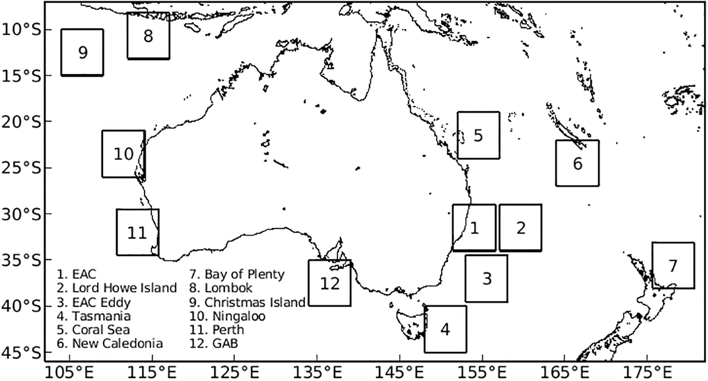
Map of the domains around Australia and New Zealand that are used to test analog forecasts.
The most computationally intensive step in our system is reading the archived data into memory. This is made more efficient by “cutting out” regional subsets of each model in advance for each domain.
2.3 Analysis of the model archive
As noted in the introduction, most NWP centres have abandoned analog forecasting, citing the difficulty finding “good analogs”. Here, we use data from many different sources, hoping to expand the catalogue of states from which analogs can be identified. The full aggregated archive of states is assembled from 16 different model runs or analysis products (Table 1) from over 1000 years of data. To evaluate how data from additional sources contribute independent information to the archive, we perform a singular value decomposition (SVD) on various subsets of the archived fields. We analyse data from Region 1, which we assume to be representative of other regions. We perform the SVD for each model run or analysis product individually; and we also calculate the SVD for aggregated archives, starting with a single model run (m=1) and progressively including data from additional model runs and analysis products, up to m=16.
Since the square of each singular value of a data matrix is proportional to the variance explained by its corresponding mode, the singular value spectrum shows how the effective dimension of the state space changes with the addition of each new source of SLA data. To prevent artificial inflation of the variance due to increasing sample size, we normalise each data matrix by , where n is the number of daily fields in the archive. This normalisation ensures that increases in singular values truly reflect new patterns of variability, not simply more data. When a new dataset contributes no independent information, its addition doesn’t change the singular values; and the data from the new source merely projects onto existing modes. By contrast, an increase in singular values indicates an increase in the effective dimension of the subspace spanned by the archive.
Results are presented in Figure 2, showing the spectra of singular values for: (a) all OFAM runs, (b) both ocean analyses, (c) all ACCESS-OM2–01 runs, and (d) all model runs and analyses listed in Table 1. In Figure 2a, although six OFAM runs are included, they fall into three distinct groups with independent variability: the ERA-Interim–forced run (EISP), the JRA-55–forced runs (JRSP, Y79R), and the reanalyses (BR20, BR23). We find that CM85 adds no new dimensions on top of EISP, JRSP, and Y79R. We also see that both reanalyses (BR20 and BR23) project onto equivalent modes, together increasing the overall dimension of the archived dataset.
Figure 2
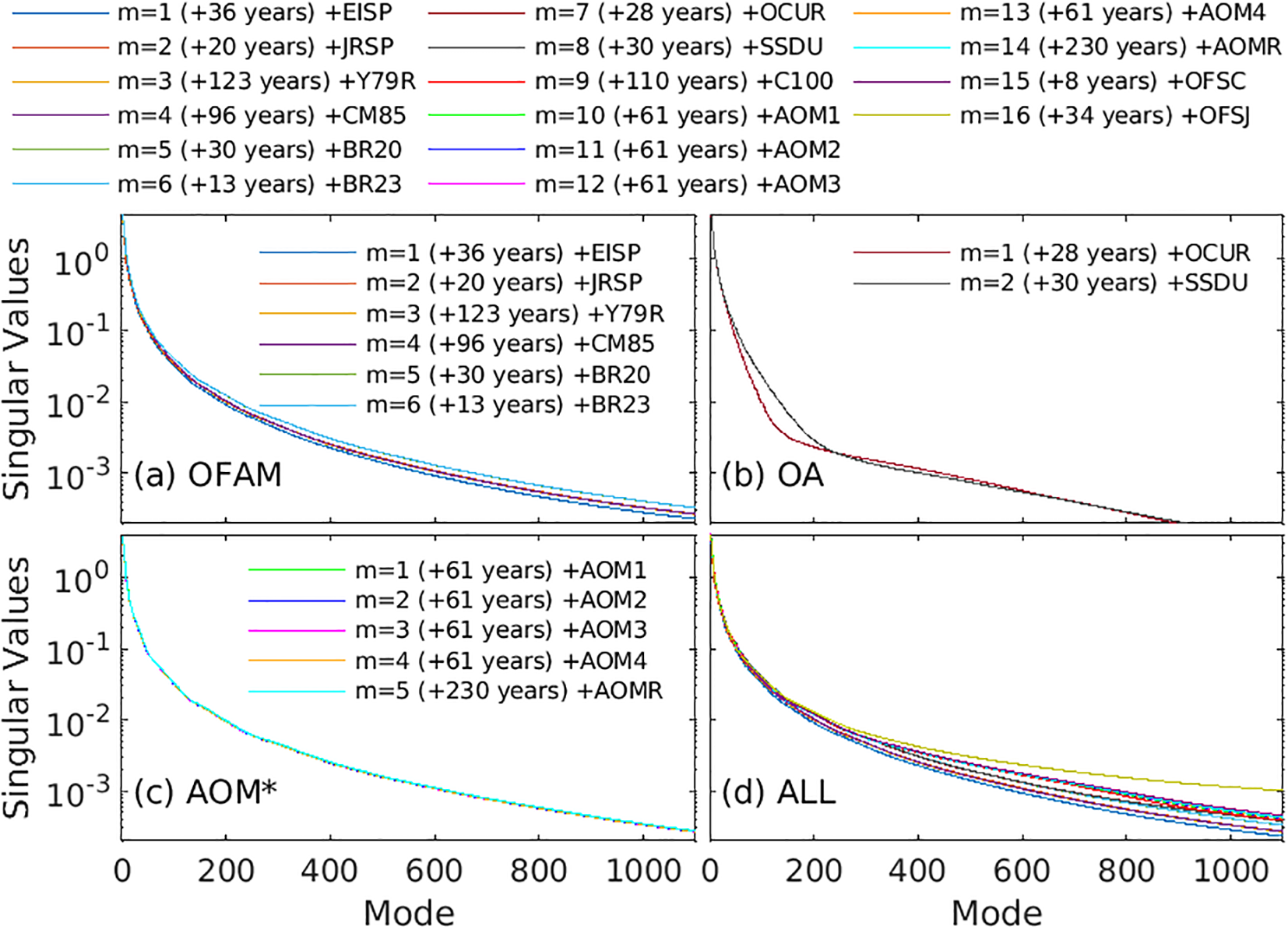
Spectrum of singular values, plotted on a log-scale, using aggregated data from 1 up to 16 model runs (for region 1), for (a) OFAM-based runs, (b) observation-based analyses, (c) ACCESS-OM2–01 based runs, and (d) all runs/analyses.
The two observation-based ocean analyses (OCUR and SSDU; Figure 2b) contribute distinct modes, likely due to differences in gridding methods and spatial resolution. All of the ACCESS-OM2–01 runs (Figure 2c) project onto the same subspace; and data from the OFES model introduces new, independent variability (Figure 2d), despite the shorter duration of those runs. We find that the C100 dataset, generated using LICOM3.0, also contributes unique modes, expanding the effective dimension of the archive.
Based on analysis of singular values (Figure 2), we conclude that multiple runs from the same model configuration generally span the same subspace. Consequently, adding more runs from the same configuration does not increase the effective dimensionality of the archive. To further explore the contribution of information to the aggregated dataset, we also examine the associated singular vectors.
We find that the right singular vectors, representing the dominant spatial modes, are effectively equivalent across all runs from the same model configuration (though the exact order of modes and the details are not precisely the same). This confirms that these runs share the same underlying spatial structures - consistent with the analysis of singular values. By contrast, the left singular vectors, representing the temporal variability, are uncorrelated across different runs - even for the repeat cycles of AOM* that span the same time periods and forced with the same fluxes. This indicates that while each run projects onto the same set of spatial modes, the combination and weighting of those modes varies in time for different runs.
The implication of this result is important: although the spatial subspace is unchanged, each new run contributes a unique combination of modes. As a result, the full set of archived fields becomes richer in its diversity of states. For analog forecasting, this means that adding more runs - even from the same model - broadens the catalogue of historical states that can be searched for analogs, increasing the likelihood of identifying a close match to the observed state.
This finding is consistent with a well-known property of high-dimensional spaces - that independently drawn random vectors from a high-dimensional state are likely to be nearly orthogonal (Christiansen, 2018). It is also supported by our sensitivity experiments that show that forecast skill consistently improves as more runs are included in the archive.
2.4 Benchmark dataset
To benchmark the skill of our analog forecasting system, we compare its predictions against archived forecasts from OceanMAPS version 4.0i (OMv4.0i; Brassington et al., 2023), accessed as they were available at the time of each forecast (last retrieved 14 February 2025). OMv4.0i is a traditional ocean forecast system that uses a hybrid-EnKF data assimilation system to initialise a near-global ocean general circulation model (OFAM). OMv4.0i uses a 48-member dynamic ensemble and a 144-member stationary ensemble, similar to Counillon et al. (2009). This approach to data assimilation combines the Ensemble Kalman Filter (Evensen, 2003) and Ensemble Optimal Interpolation (Oke et al., 2002b; Evensen, 2003; Oke et al., 2010) for estimating the system’s background error covariance. OMv4.0i produces forecasts that are of comparable performance to other operational systems run around the world (e.g., Aijaz et al., 2023) and are significantly better than version 3 of the same system that preceded it (Brassington et al., 2023).
2.5 Validation dataset
To independently assess each forecast produced here, we compare forecast SLA fields to a verifying analyses from IMOS OceanCurrent (http://oceancurrent.imos.org.au, last accessed on 14 February 2025). SLA analyses from OceanCurrent are available on a 0.2◦-resolution grid, with analyses every day. OceanCurrent analyses are produced by merging along-track SLA from all available satellite altimeter missions together with SLA observations from coastal tide gauges around Australia using optimal interpolation.
3 Method
Here, we develop a simple analog forecast system to predict SLA for a regional domain to quantify the mesoscale ocean circulation. The inputs required for this approach include an estimate of the current state of the ocean, and an archive of past or simulated ocean states. The system identifies the instance in the archive that is most similar to the current state. This instance is considered an “analog”, and the sequence of archived fields immediately following the identified analog is assembled as a forecast.
With some exceptions (e.g., Delle Monache et al., 2013; Junk et al., 2015), most analog forecasting systems identify a single forecast. Here, we extend this approach by identifying an ensemble of analogs, each representing a possible evolution of the ocean. We analyse the forecasts from each individual analog, as well as their ensemble mean. This is conceptually similar to kNN (e.g., Fix and Hodges, 1951; Cover and Hart, 1967), which often involves weighted ensemble averaging (e.g., Gul et al., 2022). Several other studies have used analog forecasting with a modified kNN approach to produce tailored weather forecasts (e.g., Bannayan and Hoogenboom, 2008; Hall et al., 2010; Xie et al., 2024). For the remainder of this study, we refer to each analog (ensemble member) as a nearest neighbour (NN).
Each NN is identified using an objective similarity metric between the observed ocean state and archived fields. Common metrics include anomaly cross-correlation (ACC) and mean absolute difference (MAD). For the application presented here we prefer using ACC as the metric for calculating similarity and have used this as the default for calculations presented in this study. The archive of past states may be sourced from a single long model run (e.g., Kiss et al., 2020), a reanalysis (e.g., Chamberlain et al., 2021b), or observation-based analyses (e.g., Ballarotta et al., 2025). Many analog forecasting studies use data from a single reanalysis or model run. However, to ensure dynamically consistent forecasts, most of the results presented in this study only use fields from free-running model simulations without data assimilation (a subset of runs listed in Table 1 - only those with run types of IAF, RYF, of CLIM; referred to below as Experiment 1).
The present ocean state is defined using satellite altimetry-derived SLA observations, which effectively capture the boundary currents and mesoscale features, such as eddies and fronts. For most experiments reported here, we use SLA data over a 10-day period, instead of just a single-day of observations. We compare the most recent 10-day evolution of SLA, relative to the analysis time (t=0), to archived sequences of the same length. This allows the system to identify analogs that best match the recent temporal variability of mesoscale ocean, an approach that is similar to Local Dynamic Analog forecasting in NWP (Hou et al., 2021).
Figure 3 illustrates this approach. The top row shows along-track SLA observations over a 10-day period. The second row presents an archive of SLA fields from a model run. The lower rows display model fields interpolated to the observation locations (using bi-linear interpolation) for each 10-day period in the archive. The MAD is computed for each sample, and the sequence with the smallest MAD is selected as the NN (i.e., the best analog). The forecast SLA is then assembled from the model fields immediately following the NN period. While Figure 3 uses MAD for NN identification, ACC can also be used, and in most cases, both metrics yield similar results.
Figure 3
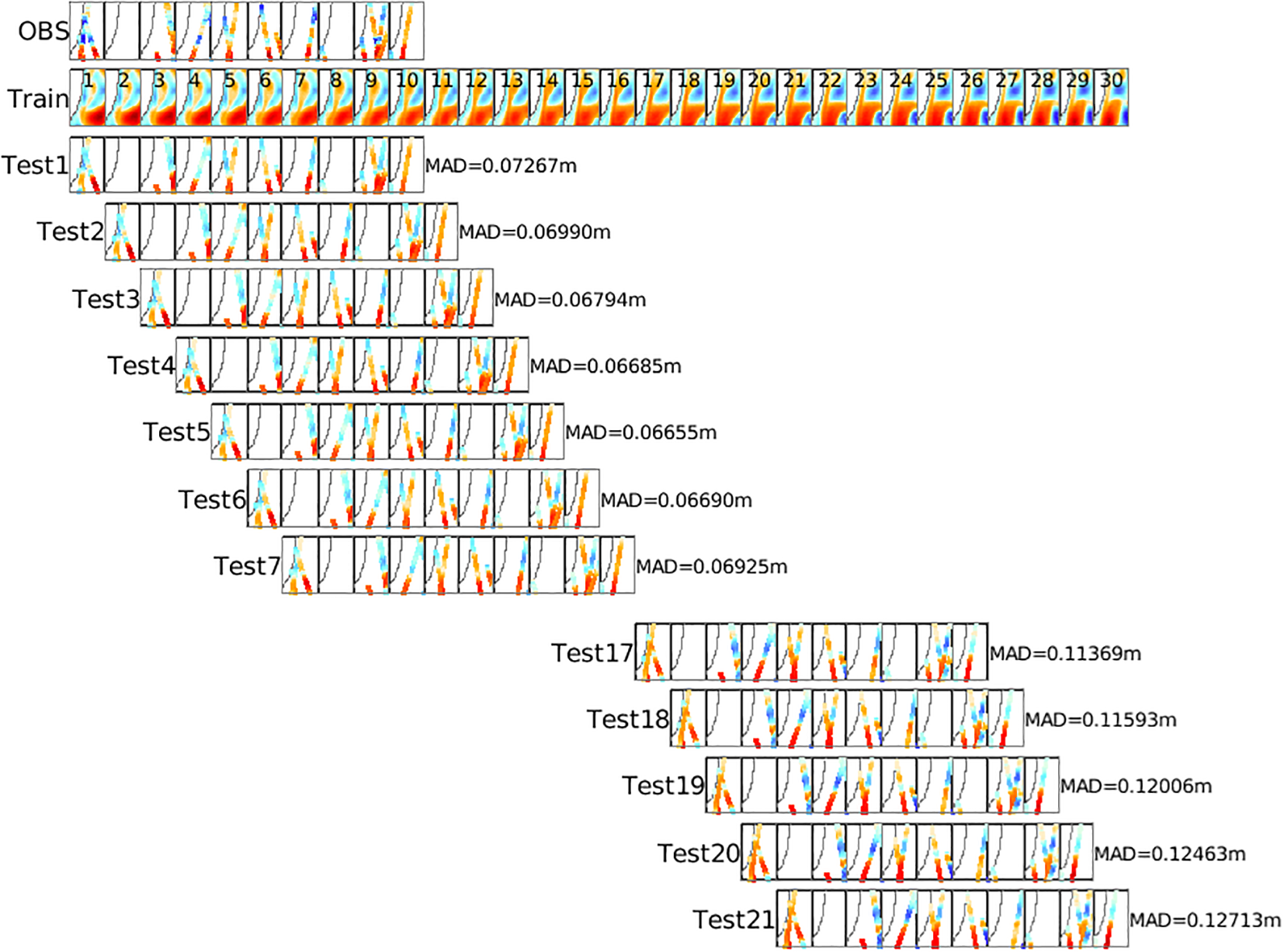
Illustration of how the analog forecast system quantifies the mean absolute difference (MAD) between a 10-day sequence of along-track altimeter observations (OBS, top row) and every 10-day sequence in the training dataset (Train, second row). The number in each panel of the Train row indicates the corresponding day in the training dataset. In the OBS row, each dot represents an observation location, with its colour indicating the observed SLA, ranging from -0.5 m (red) to 0.5 m (blue), with white representing zero. In the Test1, Test2, etc., rows, the colour of each dot represents the SLA value at the observation locations from the corresponding sequence in the training dataset. For clarity, fields for Test8–Test16 are not shown. This demonstration uses a simplified training dataset of only 30 days, whereas the experiments presented in this study utilise a much larger dataset spanning over 1000 years of daily SLA fields. The NN is identified as the 10-day sequence in the training dataset with the smallest MAD. In this example, for a 5◦ × 5◦ region off south-eastern Australia, the NN corresponds to Test5, with an MAD of 0.06655 m. This sequence consists of SLA fields from days 5 to 14 in the training dataset. The associated 15-day SLA “forecast” is then derived from the SLA fields immediately following day 14 (i.e., days 15–29 in the training dataset).
Figure 4 provides a more detailed example of how analog forecasting is used to assemble a forecast of SLA after the NN is identified. Again, the top row of Figure 4 shows observations over a 10-day period. The second row shows the SLA fields for the first NN. The third row presents model fields interpolated to observation locations – intended to demonstrate the consistency between the observed and archived SLA. The bottom row of Figure 4 displays a forecast for SLA that follows the last day of the NN period.
Figure 4
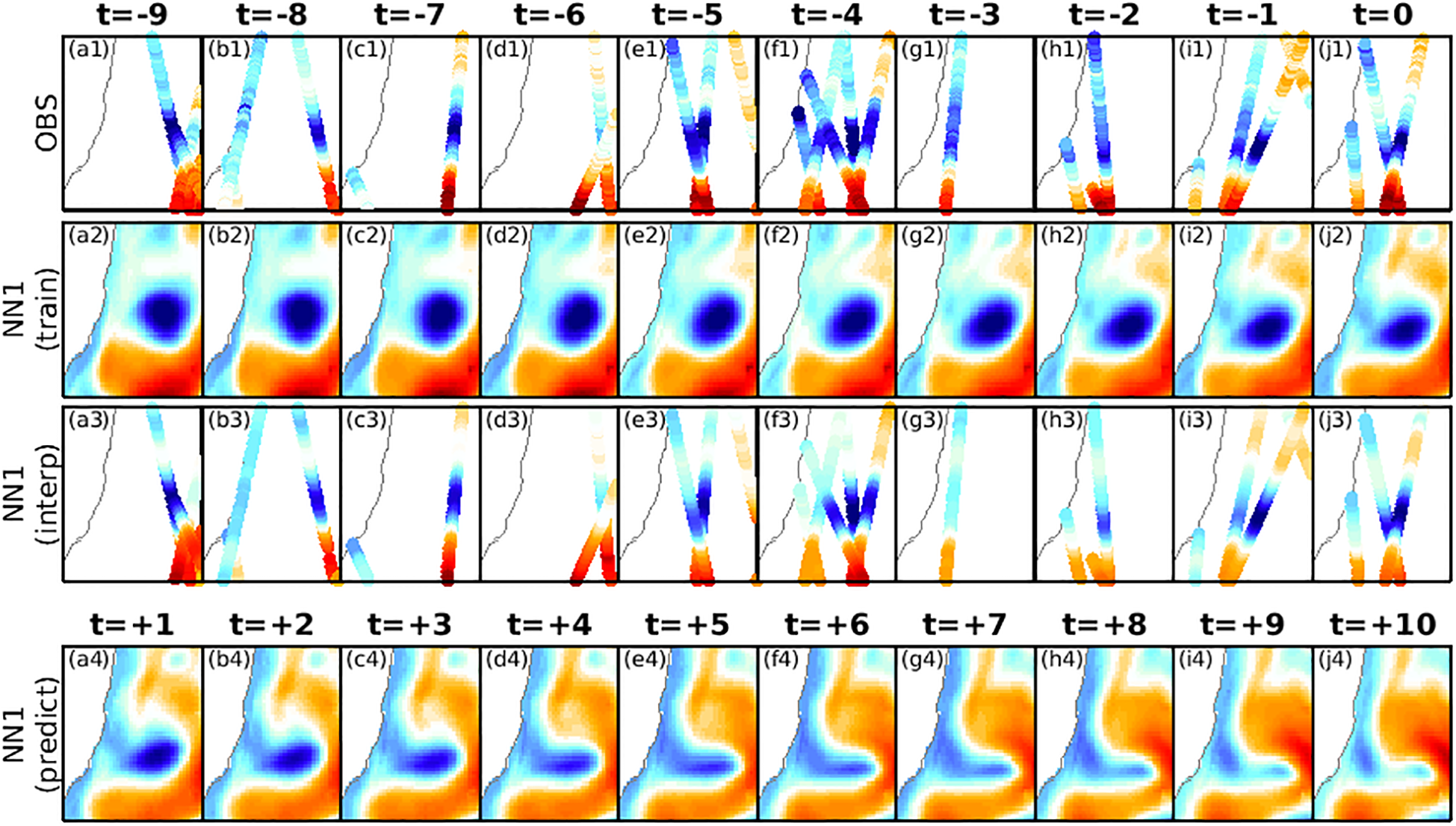
Demonstration of how a selected NN is used to produce a forecast. The top row (a1-j1) shows along-track altimeter data that is used to assess each potential neighbour, where the location of each dot denotes the location of an observation, and the colour of each dot indicated the value of the SLA observation. The second row (a2-j2) shows SLA from the archive for the first NN for the 10-day time-window that is identified to “fit” the observations most closely (for this example, the MAD of the NN is 0.0617 m and the ACC of 0.83). The third row (a3-j3) shows the modelled SLA fields interpolated to the observation locations (in time and space) – to qualitatively demonstrate the level of agreement with the observations. The bottom row (a4-j4) shows SLA for 10 days after the period selected period for the first NN – interpreted here as a 10-day forecast. This example is for a domain off south-eastern Australia, showing SLA with a range of -0.5 (blue) to 0.5 m (red), where zero is white.
In our experiments, we use an extensive archive of up to 365,502 daily SLA fields, compiled from up to 16 different sources spanning over 1000 years (Table 1). To ensure independence of each NN (each ensemble member), we apply the following selection process. First, we identify the “best” NN (NN1) - the NN with the highest ACC compared to along-track SLA. Second, we exclude all archived states within 45 days before and after NN1. Third, we identify the next best NN (NN2) and repeat until 12 NNs are selected (the choice of 12 is justified below). We’re also careful to exclude NN periods at the end of each model run, to avoid assembling a forecast that spans two different model runs. This process allows us to efficiently construct ensemble-based forecasts that are dynamically consistent and free from initialisation shock.
To evaluate the significance of the identified NNs - that is, whether the identified NNs are meaningfully distinguishable from other fields in the archive - we analyse a frequency histogram of the MAD for each 10-day period within a single forecast across six domains (Figure 5). For some domains, the histogram resembles a Gaussian distribution, while others show a skewed Gaussian shape. Some domains, such as Regions 1 and 5 have quite a long tail, suggesting that the identified NNs are truly distinct from other fields in the archive; while others, such as Regions 3 and 9, have a short tail for small values of MAD, suggesting that the NNs are not particularly distinct from many other samples in the archive.
Figure 5
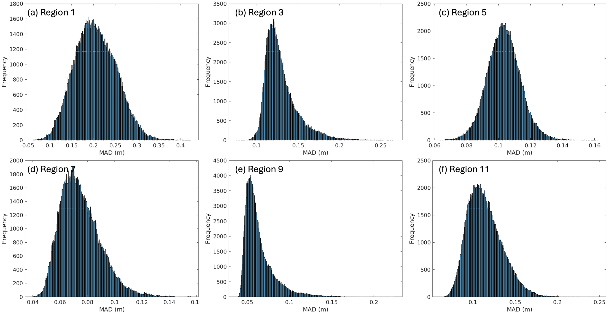
Frequency histograms of MAD for each 10-day sample tested by the kNN algorithm for an example forecast in six different domains, labelled in each panel (a-f). The NNs correspond to samples with the smallest MAD. Panel (a) shows the example represented in Figure 4. A larger tail implies more distinct NNs, compared to a random sample.
4 Results
4.1 Experiment design
To evaluate our system, we conduct 25 independent 15-day forecasts, initialised every 15 days throughout 2023. These forecasts span 12 regional domains around Australia (Figure 1), encompassing a range of dynamic regimes. Most results presented here are from Experiment 1 (Exp. 1), which uses sea level anomaly (SLA) fields from the free-running models listed in Table 1 - EISP, JRSP, Y79R, C100, AOM*, and OFS* - comprising a total of 902 years of daily SLA data.
4.2 Statistical assessment
Figures 6 , 7 summarise the system performance across all domains. Figure 6 compares MAD between SLA in the verifying analysis and forecasts from three sources, including the kNN-based equal-weighted ensemble mean (kNN EqW); OceanMAPS version 4.0i (OMv4.0i); and the first nearest neighbour (NN1). Figure 7 shows an equivalent analysis, but using ACC to evaluate forecasts.
Figure 6
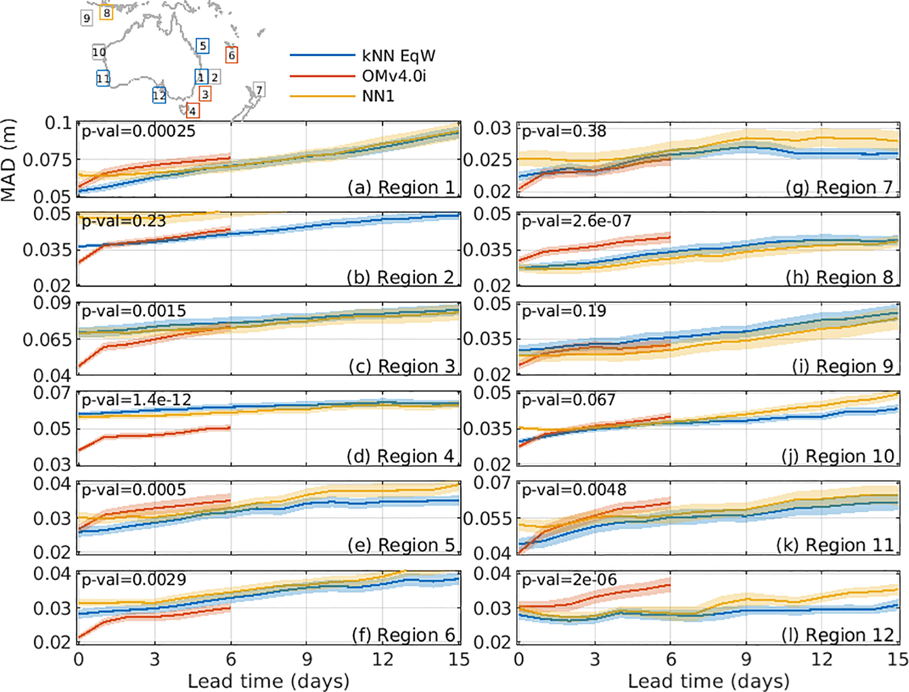
Plots showing the MAD between a verifying SLA analysis (from OceanCurrent) and predicted SLA from the ensemble mean of 12 NNs (kNN EqW, blue), OceanMAPSv4 (OMv4.0i, red), and the first NN (NN1, orange) for 12 different regions (smaller MAD is better), labelled in each panel (a-l). Each panel shows the average MAD as a function of lead time, averaged over 25 independent forecasts starting 15 days apart during 2023. Shaded areas denote the error of the mean metrics. Each panel also shows the p-value for the comparison between the forecast from either kNN EqW or NN1 (whichever is smallest) and OMv4.0i (averaged over days 1-6) and the next smallest. A p-value below 0.05 indicates that such a difference would occur by chance less than 5% of the time under the null hypothesis of equal performance. The location of each domain is indicated by the region number, referenced to the map at the top left and in Figure 1. Boxes with p-values below 0.05 are coloured according to the forecast system that exhibited statistically significant superior performance, while grey boxes indicate domains where the mean metrics are statistically equivalent. Overall, the kNN forecasts (either kNN EqW or NN1) produced significantly smaller MAD for 5 of 12 domains, whereas OMv4.0i gave the best forecasts for 3 of 12 domains.
Figure 7
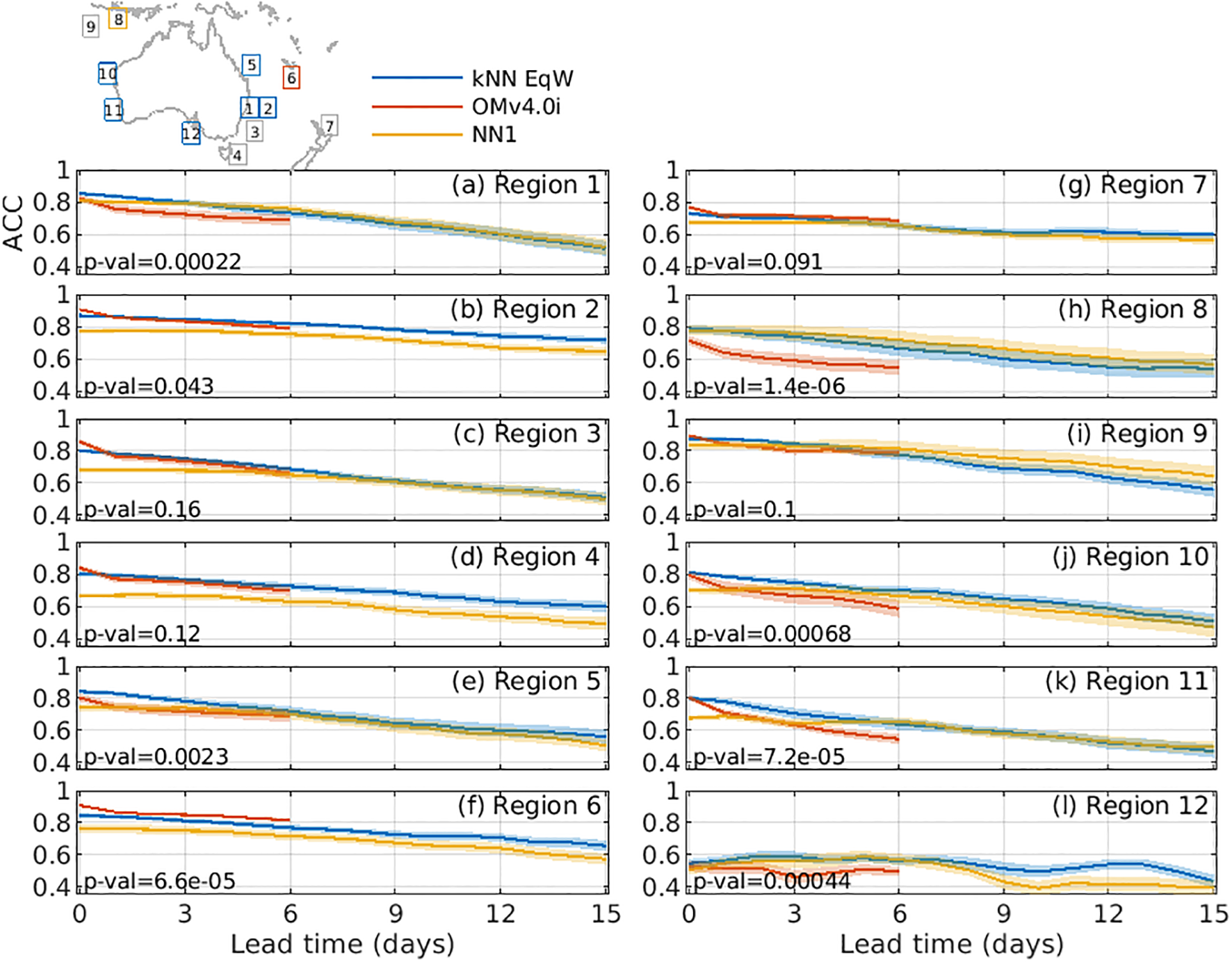
(a-l) As for Figure 6, but showing ACC between a verifying SLA analysis and predicted SLA (larger values indicate better performance). Overall, kNN forecasts (either kNN EqW or NN1) yielded higher ACC in 7 of 12 domains; OMv4.0i was clearly best in 1 domain; and the mean ACC wasn’t statistically different for 4 domains, with a high chance that the differences could occur by chance.
For Figures 6, 7, we show the mean metrics computed from 25 forecasts. The shaded bands represent the standard error of the mean across those forecasts, and the associated p-values are also reported in each panel. To identify the “best” forecast performance for each region, we compare the metrics (averaged over forecast days 1-6 - limited to 6-day forecasts because that is available from OMv4.0i) between three forecast types: kNN EqW, OMv4.0i, and NN1.
For each pairwise comparison, the null hypothesis is that the two forecast methods have equal mean performance. We evaluate this hypothesis using a standard two-sample t-test (e.g., Browne, 2010) applied to the distribution of metrics across the 25 forecasts. A p-value (e.g., Vidgen and Yasseri, 2016) below 0.05 indicates that the observed difference in mean metrics would occur by chance less than 5% of the time under the null hypothesis. When the p-value is below this threshold, we regard the difference between forecast methods as statistically significant.
For regions where one forecast type significantly outperforms the benchmark – or where the benchmark significantly outperforms the kNN-based forecasts – we denote the region with a coloured box in Figures 6, 7.
Using MAD as a metric, kNN EqW outperforms OMv4.0i in 4 of 12 domains, NN1 outperforms OMv4.0i in 1 of 12 domains, and OMv4.0i outperforms the kNN-based forecasts for 3 of 12 domains (Figure 6). For 3 of 12 domains, the mean MAD are not significantly different.
Using ACC, kNN EqW outperforms OMv4.0i in 6 of 12 domains; NN1 outperforms OMv4.0i in 1 of 12 domains, and OMv4.0i outperforms the kNN-based forecasts in 1 of 12 domains (Figure 7). For 4 of 12 domains, the mean ACC are not significantly different.
Based on these results, we conclude that the kNN/analog system outperforms traditional operational forecasts in 40-60% of cases, performs equally well (no statistical difference) in about 30% of cases, and is outperformed in about 10-25% of cases.
A distinct feature of OMv4.0i forecasts is a sharp increase in MAD and drop in ACC between days 0 and 1 (Figures 6, 7). We attribute this to initialisation issues that are caused by the dynamically inconsistent initial conditions, as noted in the introduction. By contrast, analog forecasts avoid such degradation since each forecast is from a free-running model, and is therefore dynamically consistent.
It is interesting to note the relative number of NNs that are identified from each source in the assembled archive (Table 2). In total, we identify 3600 NNs for this study, comprised of an ensemble of 12 for 25 forecasts over 12 domains. We report results from two configurations: Exp. 1, where only dynamically consistent SLA fields are used (from EISP, JRSP, Y79R, CM85, C100, AOM*, and OFS*); and Exp. 17, using all data in the archive (the same as Exp. 1, plus BR20, BR23, OCUR, and SSDU). For Exp. 1, we find that there is a disproportionally high number of NNs from AOM* IAF runs – accounting for 38.1% of NNs in Exp. 1, having contributed 30.3% of the archive. For Exp.17, when we include ocean reanalyses and observation-based analyses in the archive, this weighting towards the AOM* IAF runs reduces, and the observation-based analyses contribute a disproportionally large percentage of NNs. Together, OCUR and SSDU account for 11.5% of NNs, having only comprised 5.9% of the archive; and fields from the BRAN experiments account for 7.4% of NNs, having contributed only 4.4% to the archive.
Table 2
| Source | Runs | Exp. 1 | Exp. 17 | ||
|---|---|---|---|---|---|
| %NNs | %Archive | %NNs | %Archive | ||
| OFAM IAF | EISP+JRSP. | 8.6% | 6.9% | 5.6% | 5.6% |
| OFAM RA | BR20+BR23 | 0.0% | 0.0% | 7.4% | 4.4% |
| OA | OCUR+SSDU | 0.0% | 0.0% | 11.5% | 5.9% |
| OFAM RYF | CM85+Y79R | 10.0% | 15.3% | 17.3% | 21.8% |
| LICOM IAF | C100 | 11.3% | 13.6% | 8.0% | 10.8% |
| ACCESS-OM2–01 IAF | AOM1-4 | 38.1% | 30.3% | 27.3% | 24.3% |
| ACCESS-OM2–01 RYF | AOMR | 26.6% | 28.7% | 19.4% | 23.0% |
| OFES1 CLIM | OFSC | 0.5% | 1.0% | 0.4% | 0.8% |
| OFES2 RYF | OFSR | 4.9% | 4.2% | 3.1% | 3.4% |
Percentage of NNs identified from each model/source, along with the percentage of the total model archive that is from each source.
Results are shown for two experiments: Exp. 1 include archived SLA fields from EISP, JRSP, CM85, Y79R, C100, AOM*, OFSC, and OFSR; and Exp. 17 includes the same fields as Exp. 1, plus BR20, BR23, OCUR, and SSDU. The percentages in bold are when the percentage of NNs exceeds the percentage of fields in the archive.
4.3 Ensemble forecasts
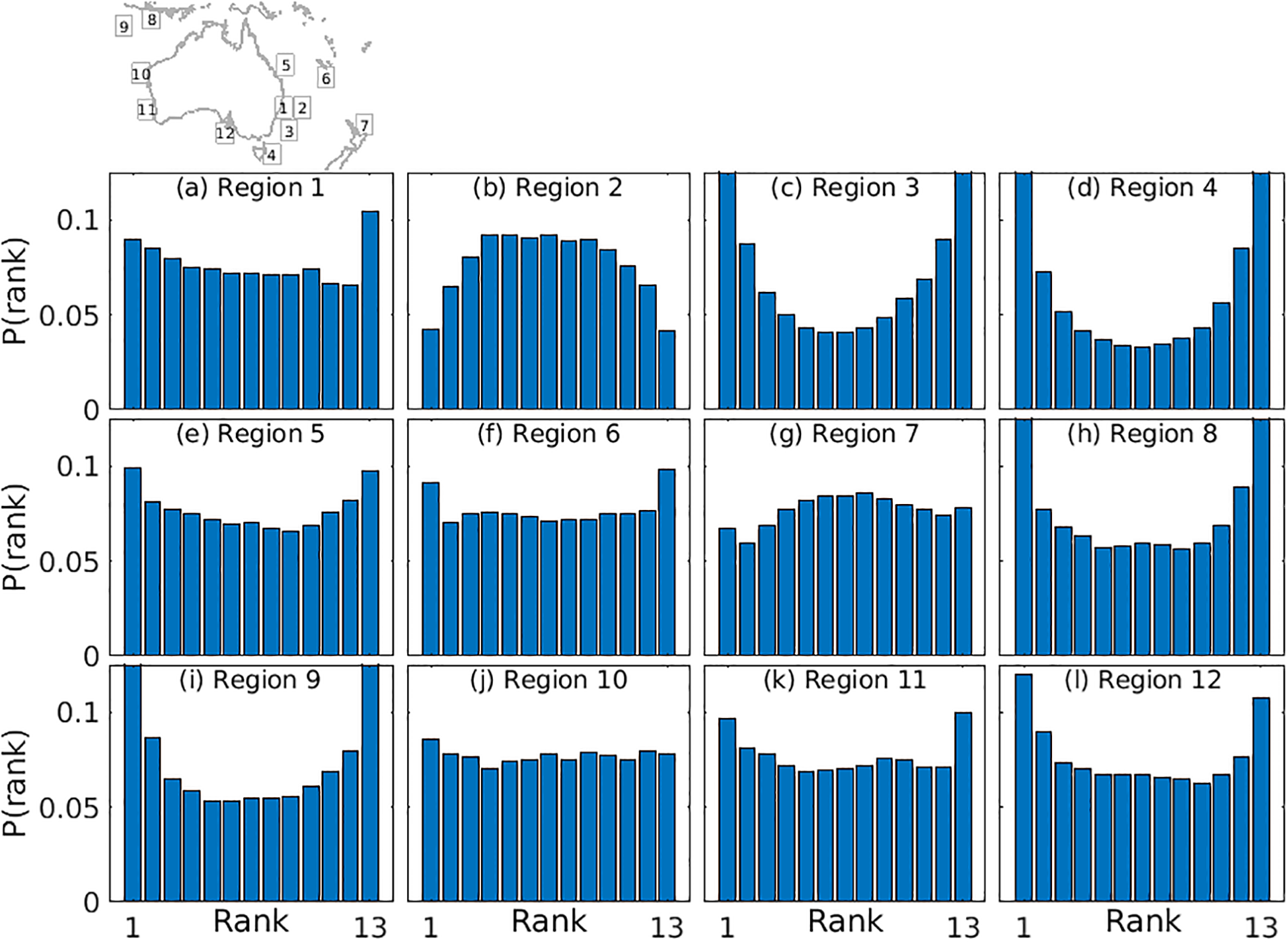
To examine the mean characteristics of the ensemble forecasts, we present mean rank histograms (Hamill, 2001) for each region – averaged over forecast days 0–15 for 25 forecasts – in Figure 8. The histograms reveal clear and spatially systematic differences in ensemble performance across the 12 regions. Several regions exhibit a pronounced U-shape (e.g., regions 3, 4, 8, and 9), indicating that the ensemble spread is generally under-dispersive and that observations frequently fall outside the ensemble range (e.g., Hamill, 2001). Region 2 displays a dome-shaped distribution, suggesting an over-dispersive ensemble. Other regions – particularly regions 6, 7, and 10 – show flatter, more uniform histograms that imply a more appropriate spread. Regions with strong skewness towards the lowest or highest ranks (e.g., regions 3, 4, 8, and 12) indicate localised biases in the ensemble mean.
Figure 8
Mean rank histograms, averaged over day 0–15 of 25 forecasts for each region, labelled in each panel (a-l).
Overall, the rank histograms indicate that the analog-based ensembles capture important aspects of forecast uncertainty, although the spread is insufficient in a number of regions and occasionally exhibits systematic skewness. These deficiencies likely reflect limitations in the diversity or representativeness of the analog archive, rather than issues associated with ensemble data assimilation. The poorest-performing regions (3, 4, 8, 9, and 12) show clear U-shaped histograms, consistent with under-dispersion. In three of these regions (3, 4, and 9), the analog ensemble usually underperforms relative to OMv4.0i (Figures 6, 7). This suggests that kNN performance could be improved by expanding or diversifying the archive so that the selected states span a broader range of independent dynamical conditions.
To further illustrate forecast performance and practical application, we present a number of detailed examples (Figures 9–13). Each example shows the verifying analyses, equal-weighted NN ensemble means, and forecasts from 12 individual NNs at t+0, t+5, t+10, and t+15. Results described in this section are from Exp. 1, using only SLA fields from free-running models. The examples discussed below include a mix of cases when the analog forecast system performs well, and some where it performs poorly. To further demonstrate the performance, we also offer results from 35 other examples (2 or 3 for each region) in the Supplementary Material.
Figure 9

Example 1: Analog forecasts for the EAC domain (Region 1, Figure 1) for a forecast starting on 2 January 2023, showing Ocean Current analyses (a-d), the equal-weighted NN ensemble mean (a0-d0), and the 12 NNs (a1-a12 – a12-d12). The source (model and model run) for each NN is indicated to the left of each sequence of NN fields, along with the month and year of each NN. SLA for are shown at (column a) t+0, (column b) t + 5d, (column c) t + 10d, and (column d) t + 15d. The ACC for the ensemble mean (black) and each NN (coloured) are shown, as a function of lead time, in panel (e).
Figure 10
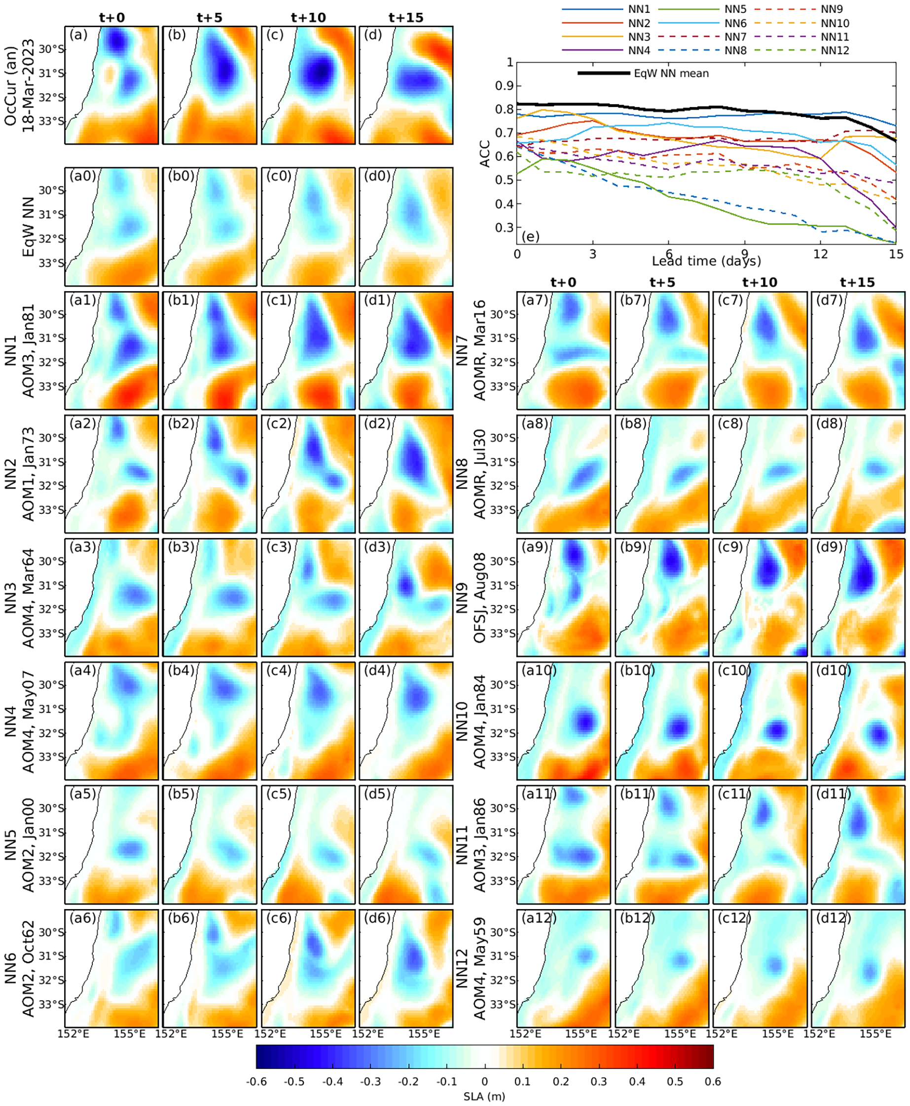
(a-d) Example 2: As for Figure 9, for the EAC domain (Region 1, Figure 1) for forecasts starting on 18 March 2023.
Figure 11
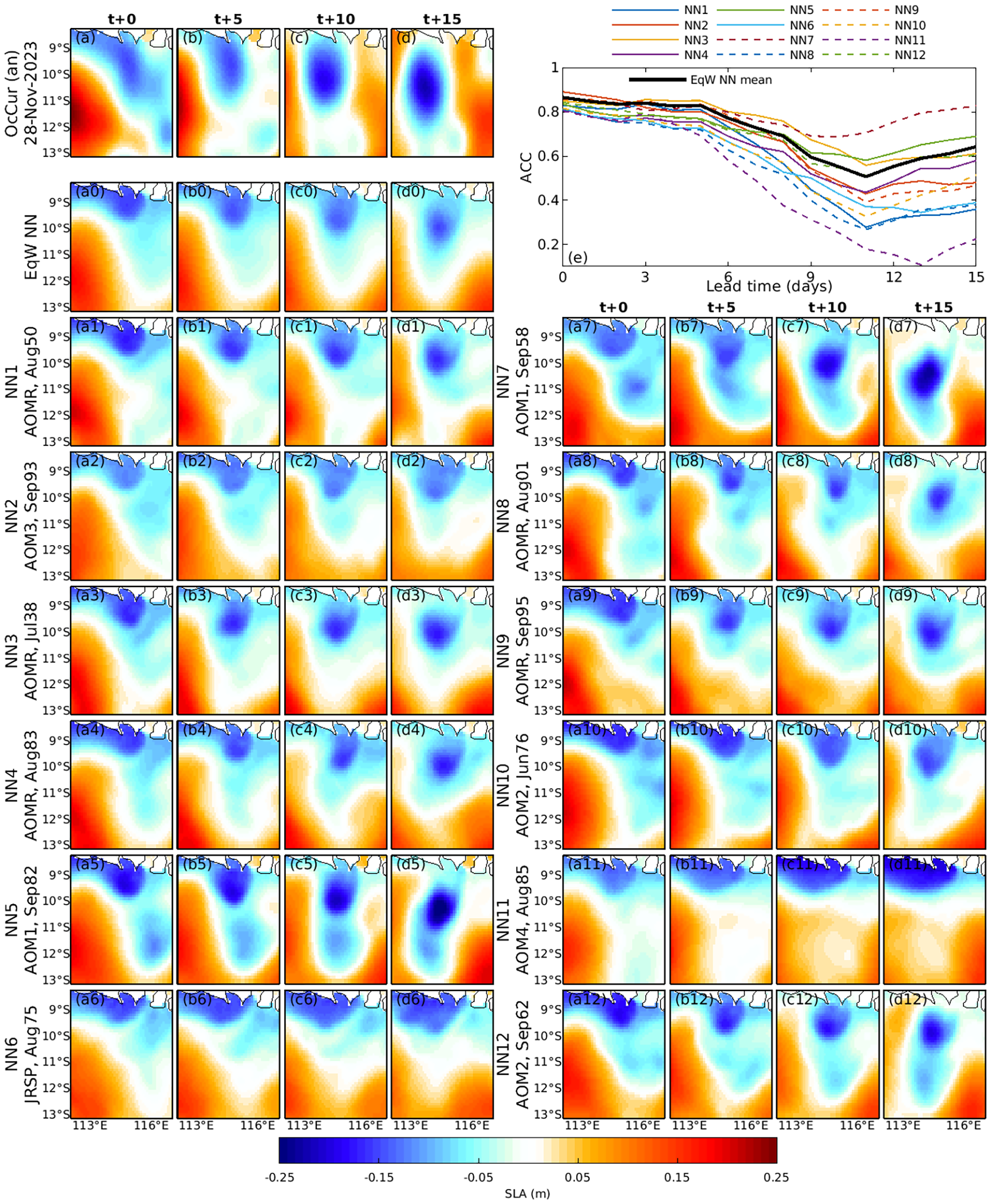
(a-d) Example 3: As for Figure 9, except for the Lombok domain (Region 8, Figure 1) for forecasts starting on 28 November 2023.
Figure 12
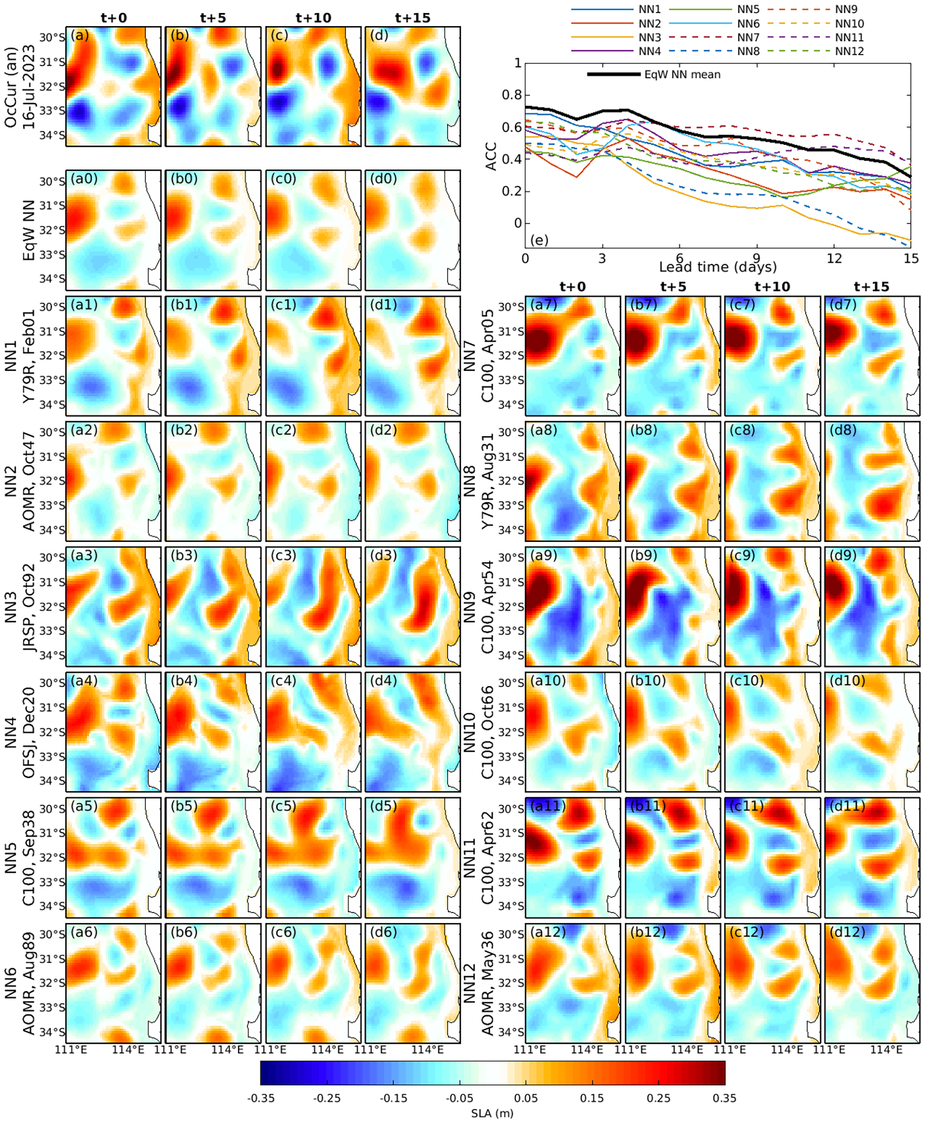
(a-d) Example 4: As for Figure 9, except for the Perth domain (Region 11, Figure 1) and for forecasts starting on 16 July 2023.
Figure 13
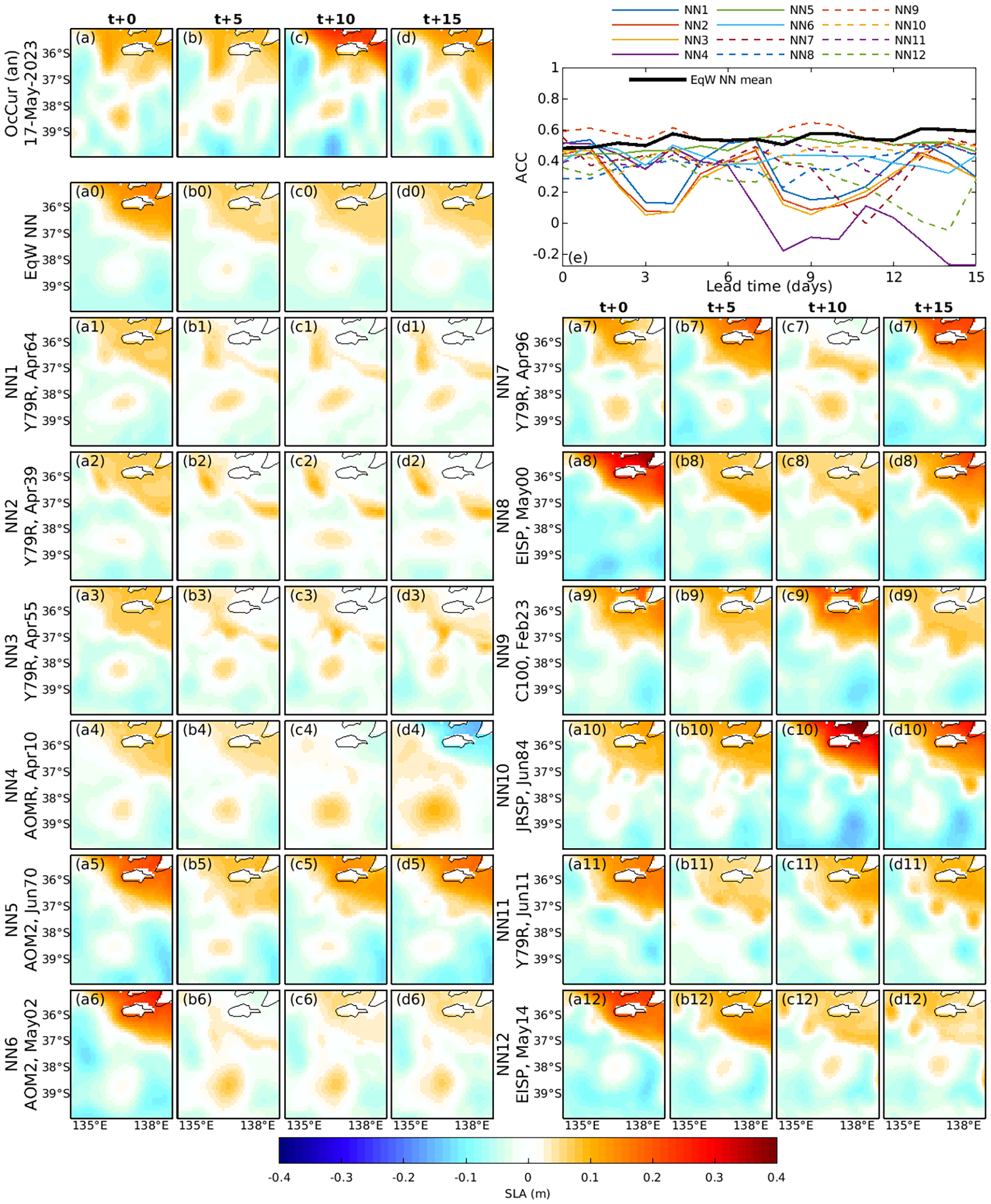
(a-d) Example 5: As for Figure 9, except for the GAB domain (Region 12, Figure 1) and for forecasts starting on 17 May 2023.
Interestingly, for most cases, the initial conditions of each NN (at t+0) are often quite different from the verifying analyses at t+0. This is not surprising, because each NN is identified based on their similarity to observed evolution over a 10-day period, not necessarily their initial state (at t+0).
4.3.1 Example 1: Eastern Australian Current Region
Figure 9 shows an ensemble forecast for the EAC domain (Region 1), initialised on 2 January 2023. The dominant feature at t+0 is a cyclonic eddy at ∼32◦S. Over the first week, this eddy splits into two smaller cyclonic eddies, one of which elongates meridionally and merges with shelf waters. By t+15, the verifying analysis shows a weakened, isotropic cyclonic eddy near 155◦E.
Several NNs (NN4, NN10, NN11, and NN12) reproduce these key features well. The verifying analysis also indicates a cyclonic feature emerging by t+10 in the northeastern corner of the domain. While NN4 and NN12 capture this feature to some extent, none of the NNs predict it accurately.
Among all forecasts, NN10 has the highest ACC at t+15 (Figure 9e), forecasting the details of the small cyclonic eddy at 32◦S, and realistically forecasting the distortion of the surrounding high-pressure system (the orange region in the south-east of the domain, Figure 9d), and the low sea level along the coast.
4.3.2 Example 2: EAC—High Variability Case
Figure 10 provides another example from the EAC domain, chosen to highlight a case where SLA undergoes significant changes during the forecast period. At t+0, two cyclonic eddies are evident in the northern half of the domain. These eddies coalesce into a single, stronger cyclonic eddy within the first 5 days and then drift southward. Only about half of the NNs (NN1, NN2, NN6, NN7, NN11) capture both initial eddies. All NNs that correctly represent these features in their initial conditions predict their coalescence. By t+15, NN1 has the highest ACC, with a correlation of about 0.7.
4.3.3 Example 3: Lombok domain
The Lombok domain (Region 8) exhibits variability that is quite different to the EAC domain. Figure 11 presents a forecast for a period when a low-pressure anomaly near Lombok Strait pinches off from the coast, forming a strong, quasi-isotropic cyclonic eddy. This development is well forecasted by most of the NNs, and is well-represented in the ensemble mean.
Again, Figure 11e shows that the most precise forecast is not from the ensemble mean and is not from NN1, but is from NN7. By t+15, the SLA forecast error for NN7 is less than 4 cm and with an ACC of over 0.8. For comparison, the SLA signal during this event exceeds 30 cm, indicating that this forecast has a small error relative to the signal.
4.3.4 Example 4: Perth Region—Complex Eddy Fields
Figure 12 shows an ensemble of SLA forecasts for the Perth domain (Region 11). This case is notable for the presence of multiple small-scale mesoscale features. At t+0, the verifying analysis includes at least five distinct mesoscale features. While many NNs contain multiple mesoscale features, most fail to match the correct intensity or precise position of all mesoscale features. This highlights one of the challenges of ocean forecasting - the problem of high dimensionality. Even using two-dimensional SLA fields, the ocean can include many small-scale features that are challenging to quantitatively reproduce in a model.
Despite the complexity in this example, some NNs – particularly NN6 and NN10 – produce forecasts that may be useful to an end user. These NNs capture most of the mesoscale features, albeit with differences in intensity and location.
In general, we expect that the analog forecasting approach may not produce reliable forecasts for this type of scenario. However, experienced end users may recognise the inherent uncertainty in such cases and adjust their expectations accordingly.
4.3.5 Example 5: Great Australian Bight
The final example (Figure 13) is for the Great Australian Bight (GAB), near the Bonney Coast (Region 12). The circulation in this region is known to be strongly wind-driven (Middleton and Bye, 2007). Because of this, we expect that selection of NNs based solely on initial conditions (or more precisely, conditions preceding t+0) will likely fail to predict developing wind-driven events. This limitation is evident in this example – with different NNs capturing wind-driven variability at different times leading to high SLA variability in the northeastern corner of the domain. However, the verifying analysis does not show this variability. This highlights a case where NN forecasting may be unsuitable. An option to try to address this could involve using forecast winds to identify NNs for wind-driven regions – though we haven’t explored this possibility.
4.3.6 Summary
These examples demonstrate the strengths and limitations of kNN and analog forecasting for predicting the mesoscale ocean circulation. While this method can effectively capture mesoscale features, NN selection based on conditions preceding t+0 alone may perform unreliably in regions dominated by wind forcing or complex eddy interactions. However, by considering forecast uncertainty and ensemble behaviour, end users may be able to interpret forecast reliability and adjust their expectations accordingly.
4.4 Sensitivity experiments
A key question in ensemble data assimilation studies relates to the optimal ensemble size. For this study, this is the same as seeking the optimal number of NNs for each forecast. The efficiency of the kNN approach readily permits performance of a comprehensive set of sensitivity tests.
For each forecast, we calculate the MAD between the ensemble mean of the first 1, 2···100 NNs and the verifying analyses (from OceanCurrent). Figure 14 shows the average MAD as a function of ensemble size, averaged over all 300 forecasts (25 forecasts across 12 domains). While no single optimal ensemble size is evident, averaging 10–25 NNs seems to produces the most accurate ensemble-mean forecast. This result guided our choice of 12 NNs for results presented in this study.
Figure 14
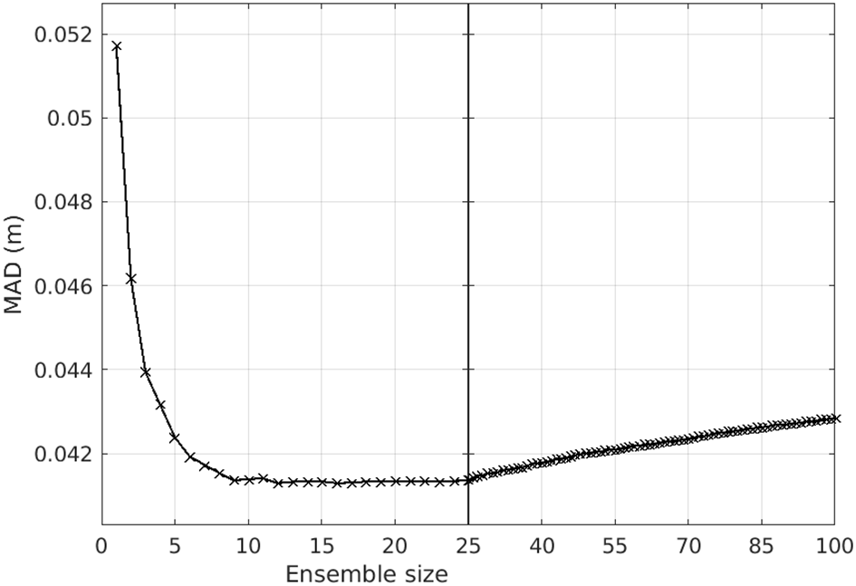
MAD plotted as a function of ensemble size. Statistics are calculated from 25 15-day forecasts for 12 domains (a total of 300 forecasts). The optimal ensemble size is not well-defined – ranging from about 9 to 20 – but the minimal average MAD is achieved with an ensemble size of 12 for the cases considered here.
Compared to traditional ocean forecast systems, there are relatively few “tuneable parameters” in an analog forecast system. However, results can be sensitive to the data included in the archive and the method used to identify NNs. We summarise a series of sensitivity experiments in Table 3. This includes experiments using different sources of SLA in the archive, using a different metric for identifying NNs, using a different observation window for identification of the NNs, and using a different ensemble size. We present these mean statistics to demonstrate the sensitivity, but we have not applied the same rigorous statistical tests that we applied the results in Figures 6, 7. Here, we aim merely to quantify the sensitivity, rather than definitively identify the “optimal” configuration.
Table 3
| Experiment | ACC | |||||||||||
|---|---|---|---|---|---|---|---|---|---|---|---|---|
| 1 | 2 | 3 | 4 | 5 | . 6 | 7 | 8 | 9 | 10 | 11 | 12 | |
| OceanMAPSv4.0i | 0.72 | 0.83 | 0.73 | 0.75 | 0.72 | 0.85* | 0.71 | 0.61 | 0.81 | 0.67 | 0.64 | 0.49 |
| Exp.1 (ACC ID w/10 d) | 0.80 | 0.84 | 0.75 | 0.77 | 0.78 | 0.81 | 0.70 | 0.73 | 0.84 | 0.75 | 0.71 | 0.58 |
| Exp.2 (E1 w/MAD ID) | 0.78 | 0.83 | 0.72 | 0.71 | 0.77 | 0.83 | 0.71 | 0.73 | 0.82 | 0.71 | 0.71 | 0.54 |
| Exp.3 (E1 w/4d) | 0.81 | 0.84 | 0.76 | 0.77 | 0.78 | 0.80 | 0.69 | 0.72 | 0.83 | 0.77 | 0.74 | 0.55 |
| Exp.4 (E1 w/15d) | 0.77 | 0.83 | 0.71 | 0.73 | 0.76 | 0.81 | 0.69 | 0.72 | 0.80 | 0.73 | 0.70 | 0.55 |
| Exp.5 (E1 w/7d) | 0.82 | 0.85 | 0.77 | 0.77 | 0.79 | 0.80 | 0.69 | 0.75 | 0.84 | 0.75 | 0.74 | 0.56 |
| Exp.6 (E1+CM85) | 0.81 | 0.84 | 0.75 | 0.76 | 0.78 | 0.81 | 0.70 | 0.73 | 0.84 | 0.75 | 0.72 | 0.58 |
| Exp.7 (E1-Y79R-C100-OF*) | 0.77 | 0.83 | 0.75 | 0.76 | 0.78 | 0.81 | 0.69 | 0.74 | 0.83 | 0.74 | 0.69 | 0.53 |
| Exp.8 (AOM4 w/10d) | 0.73 | 0.76 | 0.69 | 0.70 | 0.74 | 0.79 | 0.64 | 0.73 | 0.79 | 0.69 | 0.69 | 0.50 |
| Exp.9 (CM85+BR*) | 0.81 | 0.85 | 0.75 | 0.77 | 0.78 | 0.81 | 0.70 | 0.74 | 0.84 | 0.74 | 0.72 | 0.58 |
| Exp.10 (E9 w/6d) | 0.82 | 0.85 | 0.77 | 0.77 | 0.79 | 0.82 | 0.70 | 0.75 | 0.83 | 0.76 | 0.73 | 0.56 |
| Exp.11 (E9 w/5d) | 0.82 | 0.83 | 0.76 | 0.77 | 0.79 | 0.82 | 0.69 | 0.73 | 0.84 | 0.77 | 0.74 | 0.58 |
| Exp.12 (E9 w/7d) | 0.83 | 0.85 | 0.77 | 0.78 | 0.79 | 0.79 | 0.70 | 0.75 | 0.84 | 0.76 | 0.73 | 0.55 |
| Exp.13 (E9 w/8d) | 0.82 | 0.85 | 0.76 | 0.77 | 0.79 | 0.80 | 0.69 | 0.74 | 0.83 | 0.76 | 0.73 | 0.55 |
| Exp.14 (E12+OC) | 0.83 | 0.85 | 0.77 | 0.78 | 0.79 | 0.79 | 0.70 | 0.76 | 0.84 | 0.76 | 0.73 | 0.55 |
| Exp.15 (E14 w/5d) | 0.82 | 0.83 | 0.76 | 0.77 | 0.79 | 0.82 | 0.69 | 0.74 | 0.84 | 0.77 | 0.74 | 0.58 |
| Exp.16 (E14 + 12/36NNs) | 0.82 | 0.85 | 0.76 | 0.78 | 0.79 | 0.81 | 0.72 | 0.77 | 0.84 | 0.76 | 0.73 | 0.58 |
| Exp.17 (E14+SD) | 0.83 | 0.85 | 0.77 | 0.77 | 0.79 | 0.79 | 0.69 | 0.76 | 0.84 | 0.76 | 0.73 | 0.55 |
| Exp.18 (E17 + 12/24NNs) | 0.82 | 0.85 | 0.76 | 0.77 | 0.80 | 0.80 | 0.71 | 0.78 | 0.84 | 0.76 | 0.74 | 0.56 |
| Exp.19 (E17 w/MAD ID) | 0.82 | 0.83 | 0.75 | 0.74 | 0.78 | 0.83 | 0.71 | 0.75 | 0.83 | 0.73 | 0.73 | 0.52 |
| Exp.20 (E17 w/MIX ID) | 0.83 | 0.84 | 0.76 | 0.75 | 0.79 | 0.80 | 0.70 | 0.76 | 0.84 | 0.75 | 0.73 | 0.55 |
| Exp.21 (E17 w/6NNs) | 0.82 | 0.84 | 0.75 | 0.76 | 0.77 | 0.76 | 0.68 | 0.76 | 0.83 | 0.74 | 0.71 | 0.54 |
| Exp.22 (E17 w/18NNs) | 0.83 | 0.85 | 0.78 | 0.78 | 0.80 | 0.79 | 0.69 | 0.76 | 0.84 | 0.76 | 0.74 | 0.56 |
Average ACC for forecast day 1–6 for each forecast experiment and for each domain.
The “best” result from the analog forecast system for each domain is bold; and domains where OceanMAPSv4.0i produced the best forecasts are denoted by an asterisk. Experiment 1 includes data from 11 runs in the archive (EISP, JRSP, Y79R, C100, AOM1, AOM2, AOM3, AOM4, AOMR, OFSC, OFSJ), uses a 10-day observation window to identify NNs, and uses ACC to identify NNs (ACC ID). The differences from Experiment 1 are denoted in the first column (e.g., “E9 w/7d” means the same as Exp. 9, but with a 7 day observational window to identify NNs; “+CM85” means the same as Exp. 1, expect with data from CM85 in the archive; and “-Y79R” means the same as Exp. 1, except without data from Y79R in the archive).
Several general conclusions can be drawn from these sensitivity experiments. The observation window used for identifying NNs influences the forecast skill. Comparing experiments with an observation window of 4d (Exp. 3), 7d (Exp. 5), 10d (Exp. 1), and 15d (Exp. 4), suggests that 15d is too long, and 4d is too short. Further, we conclude that a 7d window produces the best forecasts. Inclusion of SLA data from additional, or fewer, sources in the archive also influences the forecast skill. We also find that there is some improvement when a larger ensemble is used – though a more comprehensive assessment is warranted to strongly support this claim. Compare results with 12 members (Exp. 17), 6 members (Exp. 21), and 18 members (Exp. 22). For most cases, the results are intuitive, with inclusion of more data improving the forecast skill, and using less data degrading the forecast skill.
Overall, we find some sensitivities to different choices of configuration of the analog forecast system. Different domains seem to warrant different configurations. Noting the computational efficiency of this system, it’s possible that every individual domain could be tuned for the best performance. However, we also note that the range of ACC for experiments presented in Table 3 is small, so the improvement in forecast skill gained by tuning is not great. In fact, most of the differences reported here are not statistically significant, again highlighting the insensitivity of the kNN/analog approach to these choices.
5 Discussion
5.1 Advantages of analog forecasting
Although kNN or analog forecasting is not yet widely used in oceanography, this study demonstrates its significant potential for mesoscale ocean forecasting. Compared to traditional ocean forecast systems, analog forecasting offers several advantages.
First, analog forecasting can produce dynamically consistent forecasts, avoiding the rapid degradation often seen with sequential data assimilation. This may be particularly beneficial for scenarios that are sensitive to dynamical imbalance, including forecasts of the mesoscale ocean circulation (e.g., Pilo et al., 2018) and biogeochemical (BGC) forecasting (e.g., Raghukumar et al., 2015). Analog forecasting can completely mitigate these issues by ensuring dynamic consistency in the forecast fields.
Second, analog forecasting allows targeted predictions for a subset of ocean variables (e.g., SLA, SST, or surface phytoplankton) without requiring a full ocean state to be predicted for every forecast. In this study, we chose to forecast only SLA, making our system computational efficiency, but still relevant to a number of end users. By contrast, traditional numerical models have to compute the entire ocean state for each forecast, even if the intent of the system is to forecast a subset of variables (e.g., SLA in one region).
Third, our approach is efficient and cost-effective. We generated an ensemble of 15-day forecasts for a 5◦ × 5◦ domain in about 90 seconds using a modest virtual machine (with 4 Intel Xeon Gold 6430 cores and 14 GB RAM under VMware virtualization). By contrast, OceanMAPS4.0i, the operational forecast system used for benchmarking, requires approximately 7,000 CPU hours (or 420,000 CPU minutes) to generate a global 6-day forecast, as reported in the 2023 OceanPredict National Report. The results in this study, for example, used 25 global OceanMAPS forecasts that were produced on a high-performance super-computer and required almost 20 CPU years to complete; and 300 regional analog forecasts (12 domains by 25 forecasts), required about 7.5 CPU hours. The computational cost of our analog approach is therefore about 25,000 times less than a traditional ocean forecasting system for this study.
Finally, the analog method can function as a multi-system tool. The model archive can incorporate fields from different models, configurations, and resolutions (Table 1). Since all models exhibit some systematic biases (e.g., excessive mixing, misplaced boundary currents, deep mixed layers), including multiple models allows the system to preferentially select NNs that minimise systematic errors.
5.2 Limitations of analog forecasting
Despite its advantages, analog forecasting has several limitations. Every analog forecast is merely selected from the model archive. The system can only predict events that have analogs in the archive, meaning that extreme events (e.g., marine heatwaves) can only be forecasted if similar cases exist in the archive of model states. This limitation becomes particularly relevant under climate change, where unprecedented conditions may emerge. One potential mitigation is to incorporate model simulations forced by future climate projections (e.g., CM85, C100; Table 1).
Another limitation is the dependence on observation quality and availability. If observations are sparse or lack adequate spatiotemporal coverage, selected NNs may be suboptimal, degrading forecast skill. To mitigate this, we used a 10-day sequence of observations for NN selection. Incorporating additional observation types (e.g., satellite SST or Argo profiles) is another avenue for improvement, as is combining analog forecasting with other model-data synthesis techniques (e.g., Rykova, 2023).
Moreover, analog forecasting is best suited for regional domains. Applying it at global or even basin scale is impractical due to the high dimensionality of ocean states. kNN methods are known to become unstable in high-dimensional spaces (e.g., Pestov, 2013). For this study, we performed experiments to systematically test domain sizes (from 3◦ × 3◦ to 10◦ × 10◦) and found that smaller domains generally yield more accurate forecasts. A 5◦ × 5◦ domain was chosen to balance accuracy and usability (i.e., we expect that a forecast on 500x500 km domain will be useful for many end users).
Global applications of analog forecasting would seem out of reach. Such an approach would require mesoscale features (e.g., eddies) across multiple ocean regimes to align, which is unlikely. Lorenz (1969) faced a similar issue when searching for analogs in atmospheric forecasting that included the entire northern hemisphere, noting that “there are numerous mediocre analogs but no truly good ones”. While global applications seem unrealistic, regional implementations show good potential.
5.3 Model archive considerations
The archive of SLA fields used here (Table 1) are mostly from models, and mostly include two types of model runs - simulations with IAF and climatological, or RYF. Our results (Table 2) suggest that interannual forcing yields better performance for analog forecasting, though fields from climatological runs remain valuable given the chaotic nature of mesoscale circulation.
Currently, all models in our archive are based on the MOM. Expanding the archive to include simulations from other models such as NEMO (Madec, 2016), the MIT GCM (Adcroft et al., 2004), or HYCOM (Chassignet et al., 2007) could further improve forecast skill.
Although most of the results presented in this study use SLA fields from free-running models, with no data assimilation, we have also performed forecasts using fields from ocean reanalyses and observation-based analyses (Tables 1-3). When these additional sources are included, we find that many NNs are identified from these datasets (Table 2) and the forecast skill typically improved (Table 3). Close inspection of the ensuring forecasts from these sources (not shown) expose the problems with these datasets - often with noticeable discontinuities in SLA over the forecast period. The tradeoff between improved forecast skill and dynamical inconsistent forecasts is something that needs to be considered for any application.
5.4 Selection of NNs
In our experiments, we chose to use ACC between along-track altimetry and model SLA fields to select NNs. We also ran a comprehensive set of experiments using MAD, which yielded similar selections. However, forecasts using ACC to select NNs resulted in better agreement with verifying analyses.
For SLA forecasting, we think ACC is the most appropriate metric because the primary goal of the system is to provide qualitative guidance. In this context, accurately predicting the location, size, and shape of mesoscale features is more important than precisely matching their amplitude, or the amplitude of SLA over a broader area.
The most commonly used error metrics are MAD, Mean Squared Difference (MSD), and ACC. These metrics are mathematically related. For a Gaussian sample, MSD ≈ π/2 MAD2. Furthermore, MSD can be formally expressed in terms of ACC. The MSD (Equation 1) between two vectors X and Y can be expressed as:
where MSD is the mean squared difference, is the bias, and and are standard deviations of and (e.g., Murphy, 1996; Oke et al., 2002a).
These relationships indicate that selecting NNs based on MAD (or MSD) implicitly incorporates comparisons of mean fields (close to zero in this case, since SLA is an anomaly); the amplitude of mesoscale features (quantified by standard deviation); and the location and shape of mesoscale features (quantified by the ACC). Since our objective is to produce forecasts that qualitatively inform decision making, we prioritise ACC for selecting NNs, as it better captures the spatial structure of mesoscale variability.
5.5 Comparison with ensemble data assimilation
While kNN and analog forecasting are not widely used in ocean forecasting, the approach shares similarities with ensemble data assimilation methods. It can be shown that a field of increments from EnOI- or EnKF-based systems can be expressed as a linear combination of ensemble anomalies (e.g., Oke et al., 2007, 2021). Moreover, one of the key advantages of EnKF over EnOI is that the EnKF generates ensemble members that are relevant to the current forecast (e.g., Sakov and Oke, 2008), sometimes called the “errors of the day” (e.g., O’Kane et al., 2011). An analog system also produces an ensemble mean of NNs (ensemble members) that are relevant to the current state. Here, we combine these NNs to produce an ensemble mean – a linear combination of members. We can therefore see that in this way, this approach is similar to EnOI and EnKF, but at a fraction of the computational cost. However, unlike EnOI or the EnKF, analog forecasting does not exploit this ensemble to assimilate data. An ensemble of analog forecasts are merely intended to produce multiple estimates of possible future conditions.
When ensembles are used by traditional forecast systems, the ensemble is used both as an ensemble prediction, and to quantify the system’s error covariance, for data assimilation. When used for data assimilation, the system generally performs better when a large ensemble is used (e.g., Mitchell et al., 2002). While this may also be useful for ensemble prediction, the quantity of forecasts may become unmanageable for users to exploit.
5.6 Interpreting ensembles
In ensemble forecasting, the ensemble mean is often considered the primary output (e.g., Counillon et al., 2009; Sakov and Sandery, 2015; Aijaz et al., 2023). However, as shown in Figures 9-13, individual ensemble members can provide valuable insight, particularly for mesoscale feature prediction.
End users may benefit from considering both the ensemble mean and individual forecasts. A key question is whether the ensemble mean is always the best metric for assessing forecast skill. The goal of an ensemble forecast is to represent a range of plausible future states. Even if the ensemble mean is inaccurate, the system succeeds if at least one ensemble member closely matches reality. This perspective is common in atmospheric forecasting and could be more widely adopted in oceanography.
For many of the examples presented here (Figures 9-13 and in the Supplementary Material), the most skilful forecast is often one of the NNs, not the ensemble mean of NNs. This may be true for traditional ensemble data assimilation systems, and is something that warrants consideration.
5.7 On the value of forecasting a subset of the ocean state
In this study, we demonstrate that analog forecasts can outperform traditional forecasts for a subset of variables. Applications to NWP drew similar conclusions (e.g., Langmack et al., 2012; Nagarajan et al., 2015). Here, we consider the potential value of forecasting only a subset of the ocean state, compared to the entire state. Many marine industries rely on ocean forecasts to guide decision-making (e.g., Kourafalou et al., 2015; Schiller et al., 2020; Rautenbach and Blair, 2021; Ciliberti et al., 2023; Spillman et al., 2025). Most forecasts provided by national weather centres offer a comprehensive suite of data and products (e.g., Brassington et al., 2023). However, many end users do not fully exploit these forecasts. Instead, they tend to make decisions based on qualitative assessments – simply analysing images of predicted conditions (e.g., Höllt et al., 2013; Kuonen et al., 2019; Spillman et al., 2025) or considering indices that summarise broad-scale conditions (e.g., Kumar et al., 2014; Siedlecki et al., 2023), and making modest adjustments to their plans. This is especially true for industries sensitive to mesoscale ocean variability, including oil and gas, fisheries, search and rescue, shipping, and Defence.
For example, the operator of a fishing vessel might target a specific ocean feature, such as a cyclonic eddy. Their interest is likely in the location and intensity of a specific eddy (e.g., Xing et al., 2023). A shipping company might seek deviations from a direct port-to-port route, modestly adjusting their path only if favourable conditions are likely (e.g., Dickson et al., 2019). In search and rescue, identifying the current and near-future direction of surface currents is likely most crucial (e.g., Rosebrock et al., 2015). For defence, the presence or absence of strong mesoscale features could present risks or opportunities in undersea warfare (e.g., Bub et al., 2014). Oil and gas operations may need to anticipate strong currents that could jeopardise exploratory activities or to support incidents like oil spill response (e.g., Lubchenco et al., 2012). Most of these considerations may be associated with strong mesoscale eddies in their area of operation. For all these applications, a reliable forecast of SLA, from which estimates of geostrophic currents can readily be calculated, is likely to be valuable. Moreover, for many applications, a detailed forecast of subsurface properties may be unnecessary. Analog forecasting offers an approach that allows a subset of variables to be predicted, and may be a sensible option for many applications.
6 Psuedo-code
The code for performing a kNN/analog forecast is uncomplicated. We present the pseudo-code for this system below, including each step to initialise the system, identify the NNs, and evaluate each forecast.
Pseudo-code for kNN/analog system
1. Initialise experiment
-
- Load experiment parameters (e.g., variable, archive datasets, etc.).
-
- Load archive metadata.
-
- Set region loop.
2. For each region:
2.1 Load archive
-
- For each archived dataset (i.e., model runs):
-
* Read time, grid, variable.
-
* Remove times overlapping verification.
-
* Convert to anomalies if needed (subtract temporal mean).
-
* Interpolate to common grid if needed.
-
-
- Concatenate all datasets into archive.
2.2 Load verifying analysis grid
-
- Read OceanCurrent time, grid, variable.
-
- Subset to region.
3. Loop over forecasts:
For each forecast initialisation time:
3.1 Compute archive-observation similarity
-
- For each archive time:
-
* Interpolate archive to observation locations.
-
* Compute MAD and ACC.
-
* Mask archive times near gaps between datasets.
-
3.2 Select nearest neighbours
-
- Identify NN1 as the sequence with the highest ACC or lowest MAD.
-
- Exclude archive elements within 45 days of NN1, and identify NN2.
- Repeat for k NNs, where is the ensemble size.
3.3 Assemble ensemble forecasts
-
- For each NN and lead time, extract SLA field.
-
- Build 4D ensemble array.
3.4 Compute ensemble forecasts
-
- Equal-weight (kNN EqW) forecast.
-
- Load benchmark (OMv4.0i) for comparison.
3.5 Evaluate skill statistics for all lead times (0–15 days) for kNN and OMv4.0i.
-
- Compute ACC and MAD for ensemble mean.
-
- Compute ACC and MAD for each NN (ensemble member).
3.6 Rank histograms
-
- Compare verifying SLA to ensemble.
-
- Construct and store rank histogram.
3.7 Save outputs
-
- Save derived data (metrics, histograms, NN indices, etc.).
-
- Optional plots.
4. After all forecasts:
-
- Average statistics across all dates.
-
- Save summary figures and data files.
End.
7 Conclusions
Analog forecasting has been successfully applied in NWP (e.g., Bagtasa, 2021) and seasonal forecasting (e.g., Walsh et al., 2021). Similarly, kNN has a long history in classification and pattern recognition (e.g., Fix and Hodges, 1951; Hattori and Takahashi, 1999). In this study, we develop a kNN-based analog forecast system to predict regional SLA and demonstrated that this simple, computationally efficient approach can outperform traditional ocean forecast systems in many cases. Our results highlight the potential of analog forecasting as a complementary or alternative tool for mesoscale ocean prediction.
The kNN-based forecasting system may benefit end users whose decisions depend on mesoscale ocean features, such as eddies and boundary currents. This might include industries whose operations are sensitive to the location, strength, and evolution of eddies; to the location and intensity of fronts, and to the position and intensity of boundary currents. This includes industries such as fisheries, offshore energy, and shipping. Given its efficiency, adaptability and performance, analog forecasting represents a promising direction for future operational ocean forecasting.
Statements
Data availability statement
RADS satellite altimeter data are available at http://rads.tudelft.nl, with associated software at https://github.com/remkos/rads (last accessed on 26 March 2025). Data from ACCESS-OM2–01 are available from https://doi.org/10.4225/41/5a2dc8543105a (last accessed on 26 January 2025). Data from OFAM runs are available from https://thredds.nci.org.au/thredds/catalog/gb6/OFAM3/OFAM3_EI_SPINUP/catalog.html and https://dapds00.nci.org.au/thredds/catalog/gb6/OFAM3/OFAM3_BGC_2021/OUTPUT/catalog.html (last accessed on 28 January 2025). Data from the LICOM3 run are available at the Science Data Bank at https://doi.org/10.11922/sciencedb.j00076.00095 (last accessed on 17 January 2025). OFES data are accessed from https://apdrc.soest.hawaii.edu/datadoc/ofes/clim_0.1_global_1day.php (last accessed on 26 February 2025). OceanMAPS analyses and forecasts were accessed from the Australian Bureau of Meteorology at ftp://ftp-reg.cloud.bom.gov.au/register/username/nwp at the time of each forecast and archived at CSIRO (last accessed on 19 February 2025). Analyses from IMOS OceanCurrent are available from http://imos.aodn.org.au/oceancurrent (last accessed on 26 March 2025). The Ssalto/Duacs altimeter products were produced and distributed by the Copernicus Marine and Environment Monitoring Service (CMEMS) https://marine.copernicus.eu/ (last accessed on 2 April 2025).
Author contributions
PO: Conceptualization, Formal analysis, Methodology, Software, Validation, Visualization, Writing – original draft, Writing – review & editing. TR: Conceptualization, Formal analysis, Methodology, Writing – review & editing.
Funding
The author(s) declared financial support was received for this work and/or its publication. This work was supported by CSIRO.
Acknowledgments
The authors offer sincere thanks to M. Chamberlain and A. Kiss for helping us identify and access model runs produced under Bluelink (https://research.csiro.au/bluelink/) and COSIMA (https://cosima.org.au), respectively; and to H. Sasaki for helping us access OFES data (https://www.jamstec.go.jp/ofes/). The authors also gratefully acknowledge R. Woodham and M. Chamberlain for comments that led to improvements in this study.
Conflict of interest
The authors declare that the research was conducted in the absence of any commercial or financial relationships that could be construed as a potential conflict of interest.
Generative AI statement
The author(s) declare that no Generative AI was used in the creation of this manuscript.
Any alternative text (alt text) provided alongside figures in this article has been generated by Frontiers with the support of artificial intelligence and reasonable efforts have been made to ensure accuracy, including review by the authors wherever possible. If you identify any issues, please contact us.
Publisher’s note
All claims expressed in this article are solely those of the authors and do not necessarily represent those of their affiliated organizations, or those of the publisher, the editors and the reviewers. Any product that may be evaluated in this article, or claim that may be made by its manufacturer, is not guaranteed or endorsed by the publisher.
Supplementary material
The Supplementary Material for this article can be found online at: https://www.frontiersin.org/articles/10.3389/fmars.2025.1729116/full#supplementary-material
References
1
Acosta Navarro J. C. Aranyossy A. De Luca P. Donat M. G. Hrast Essenfelder A. Mahmood R. et al . (2025). Seamless seasonal to multi-annual predictions of temperature and standardized precipitation index by constraining transient climate model simulations. EGUsphere2025, 1–24. doi: 10.5194/esd-16-1723-2025
2
Adcroft A. Hill C. Campin J.-M. Marshall J. Heimbach P. (2004). “ Overview of the formulation and numerics of the MIT GCM,” in Proceedings of the ECMWF seminar series on Numerical Methods, Recent developments in numerical methods for atmosphere and ocean modellingShinfield Park, Reading, UK: ECMWF, 139–149.
3
Aijaz S. Brassington G. B. Divakaran P. Régnier C. Drévillon M. Maksymczuk J. et al . (2023). Verification and intercomparison of global ocean Eulerian near-surface currents. Ocean. Model.186, 102241. doi: 10.1016/j.ocemod.2023.102241
4
Arango H. G. Levin J. Wilkin J. Moore A. M. (2023). 4D-Var data assimilation in a nested model of the Mid-Atlantic Bight. Ocean. Model.184, 102201. doi: 10.1016/j.ocemod.2023.102201
5
Bagtasa G. (2021). Analog forecasting of tropical cyclone rainfall in the Philippines. Weather. Climate Extremes.32, 100323. doi: 10.1016/j.wace.2021.100323
6
Ballarotta M. Ubelmann C. Bellemin-Laponnaz V. Le Guillou F. Meda G. Anadon C. et al . (2025). Integrating wide-swath altimetry data into Level-4 multi-mission maps. Ocean. Sci.21, 63–80. doi: 10.5194/os-21-63-2025
7
Balmaseda M. A. Alves O. J. Arribas A. Awaji T. Behringer D. W. Ferry N. et al . (2009). Ocean initialization for seasonal forecasts. Oceanography22, 154–159. doi: 10.5670/oceanog.2009.73
8
Balmaseda M. A. Dee D. Vidard A. Anderson D. L. (2007). A multivariate treatment of bias for sequential data assimilation: Application to the tropical oceans. Q. J. R. Meteorol. Soc.133, 167–179. doi: 10.1002/qj.12
9
Bannayan M. Hoogenboom G. (2008). Weather analogue: a tool for real-time prediction of daily weather data realizations based on a modified k-nearest neighbor approach. Environ. Model. Softw.23, 703–713. doi: 10.1016/j.envsoft.2007.09.011
10
Bergen R. E. Harnack R. P. (1982). Long-range temperature prediction using a simple analog approach. Monthly. Weather. Rev.110, 1083–1099. doi: 10.1175/1520-0493(1982)110<1083:LRTPUA>2.0.CO;2
11
Bloom S. Takacs L. da Silva A. Ledvina D. (1996). Data assimilation using incremental analysis updates. Monthly. Weather. Rev.124, 1256–1271. doi: 10.1175/1520-0493(1996)124<1256:DAUIAU>2.0.CO;2
12
Brassington G. B. Sakov P. Divakaran P. Aijaz S. Sweeney-Van Kinderen J. Huang X. et al . (2023). “ OceanMAPS v4. 0i: a global eddy resolving EnKF ocean forecasting system,” in OCEANS 2023-Limerick (Piscataway, NJ, USA: IEEE), 1–8.
13
Browne R. H. (2010). The t-test p value and its relationship to the effect size and P (X>Y). Am. Statistician.64, 30–33. doi: 10.1198/tast.2010.08261
14
Bub F. L. Mask A. C. Wood K. R. Krynen D. G. Lunde B. N. DeHAAN C. J. et al . (2014). The Navy’s application of ocean forecasting to decision support. Oceanography27, 126–137. doi: 10.5670/oceanog.2014.74
15
Burgers G. Balmaseda M. A. Vossepoel F. van Oldenborgh G. van Leeuwen P. J. (2002). Balanced ocean-data assimilation near the equator. J. Phys. Oceanogr.32, 2509–2519. doi: 10.1175/1520-0485-32.9.2509
16
Chamberlain M. Oke P. Brassington G. Sandery P. Divakaran P. Fiedler R. (2021a). Multiscale data assimilation in the Bluelink ocean reanalysis (BRAN). Ocean. Model.166, 101849. doi: 10.1016/j.ocemod.2021.101849
17
Chamberlain M. A. Oke P. R. Fiedler R. A. Beggs H. M. Brassington G. B. Divakaran P. (2021b). Next generation of bluelink ocean reanalysis with multiscale data assimilation: Bran2020. Earth Syst. Sci. Data13, 5663–5688. doi: 10.5194/essd-13-5663-2021
18
Chassignet E. P. Hurlburt H. E. Smedstad O. M. Halliwell G. R. Hogan P. J. Wallcraft A. J. et al . (2007). The HYCOM (hybrid coordinate ocean model) data assimilative system. J. Mar. Syst.65, 60–83. doi: 10.1016/j.jmarsys.2005.09.016
19
Christiansen B. (2018). Ensemble averaging and the curse of dimensionality. J. Climate31, 1587–1596. doi: 10.1175/JCLI-D-17-0197.1
20
Ciliberti S. A. Fanjul E. A. Pearlman J. Wilmer-Becker K. Bahurel P. Ardhuin F. et al . (2023). “ Evaluation of operational ocean forecasting systems from the perspective of the users and the experts,” in 7th edition of the Copernicus Ocean State Report (OSR7), Vol. 2, 1–osr7. doi: 10.5194/sp-1-osr7-2-2023
21
Counillon F. Sakov P. Bertino L. (2009). Application of a hybrid enkf-oi to ocean forecasting. Ocean. Sci.5, 389–401. doi: 10.5194/os-5-389-2009
22
Cover T. Hart P. (1967). Nearest neighbor pattern classification. IEEE Trans. Inf. Theory13, 21–27. doi: 10.1109/TIT.1967.1053964
23
Daley R. (1981). Normal mode initialization. Rev. Geophys.19, 450–468. doi: 10.1029/RG019i003p00450
24
Dee D. P. Uppala S. (2009). Variational bias correction of satellite radiance data in the ERA-interim reanalysis. Q. J. R. Meteorol. Soc.135, 1830–1841. doi: 10.1002/qj.493
25
Delle Monache L. Eckel F. A. Rife D. L. Nagarajan B. Searight K. (2013). Probabilistic weather prediction with an analog ensemble. Monthly. Weather. Rev.141, 3498–3516. doi: 10.1175/MWR-D-12-00281.1
26
Deng Z. Zhu X. Cheng D. Zong M. Zhang S. (2016). Efficient kNN classification algorithm for big data. Neurocomputing195, 143–148. doi: 10.1016/j.neucom.2015.08.112
27
Dickson T. Farr H. Sear D. Blake J. I. (2019). Uncertainty in marine weather routing. Appl. Ocean. Res.88, 138–146. doi: 10.1016/j.apor.2019.04.008
28
Ding M. Liu H. Lin P. Meng Y. Zheng W. An B. et al . (2022). A century-long eddy-resolving simulation of global oceanic large-and mesoscale state. Sci. Data9, 691. doi: 10.1038/s41597-022-01766-9
29
Ding H. Newman M. Alexander M. A. Wittenberg A. T. (2018). Skillful climate forecasts of the tropical indo-pacific ocean using model-analogs. J. Climate31, 5437–5459. doi: 10.1175/JCLI-D-17-0661.1
30
Ding H. Newman M. Alexander M. A. Wittenberg A. T. (2020). Relating CMIP5 model biases to seasonal forecast skill in the tropical Pacific. Geophys. Res. Lett.47, e2019GL086765. doi: 10.1029/2019GL086765
31
Eckel F. A. Delle Monache L. (2016). A hybrid NWP–analog ensemble. Monthly. Weather. Rev.144, 897–911. doi: 10.1175/MWR-D-15-0096.1
32
Evensen G. (2003). The ensemble kalman filter: Theoretical formulation and practical implementation. Ocean. Dynamics.53, 343–367. doi: 10.1007/s10236-003-0036-9
33
Ferry N. Parent L. Garric G. Barnier B. Jourdain N. C . (2010). Mercator global Eddy permitting ocean reanalysis GLORYS1V1: Description and results. Mercator-Ocean. Q. Newslett.36, 15–27.
34
Fix E. Hodges J. L. (1951). Discriminatory analysis, nonparametric discrimination. United. States Air. Force. School. Aviation. Med.4, February.
35
Green D. Billy J. Tapim A. (2010). Indigenous Australians’ knowledge of weather and climate. Clim. Change100, 337–354. doi: 10.1007/s10584-010-9803-z
36
Griffies S. M. (2009). Elements of MOM4p1, GFDL Ocean Group Technical Report 6. Tech. rep (Princeton, NJ, USA: NOAA/Geophysical Fluid Dynamics Laboratory).
37
Gul N. Aamir M. Aldahmani S. Khan Z. (2022). A weighted k-nearest neighbours ensemble with added accuracy and diversity. IEEE Access10, 125920–125929. doi: 10.1109/ACCESS.2022.3225682
38
Hall T. J. Thessin R. N. Bloy G. J. Mutchler C. N. (2010). Analog sky condition forecasting based on a k-nn algorithm. Weather. forecast.25, 1463–1478. doi: 10.1175/2010WAF2222372.1
39
Hamill T. M. (2001). Interpretation of rank histograms for verifying ensemble forecasts. Monthly. Weather. Rev.129, 550–560. doi: 10.1175/1520-0493(2001)129<0550:IORHFV>2.0.CO;2
40
Hamill T. M. Whitaker J. S. Mullen S. L. (2006). Reforecasts: An important dataset for improving weather predictions. Bull. Am. Meteorol. Soc.87, 33–46. doi: 10.1175/BAMS-87-1-33
41
Hattori K. Takahashi M. (1999). A new nearest-neighbor rule in the pattern classification problem. Pattern Recognit.32, 425–432. doi: 10.1016/S0031-3203(98)00097-1
42
Höllt T. Magdy A. Chen G. Gopalakrishnan G. Hoteit I. Hansen C. D. et al . (2013). “ Visual analysis of uncertainties in ocean forecasts for planning and operation of off-shore structures,” in 2013 IEEE Pacific Visualization Symposium (PacificVis). 185–192 ( IEEE). doi: 10.1109/PacificVis.2013.6596144
43
Hou Z. Li J. Wang L. Zhang Y. Liu T. (2022). Improving the forecast accuracy of ECMWF 2-m air temperature using a historical dataset. Atmosph. Res.273, 106177. doi: 10.1016/j.atmosres.2022.106177
44
Hou Z. Li J. Zuo B. (2021). Correction of monthly SST forecasts in CFSv2 using the local dynamical analog method. Weather. Forecast.36, 843–858. doi: 10.1175/WAF-D-20-0123.1
45
Houtekamer P. Derome J. (1995). Methods for ensemble prediction. Monthly. Weather. Rev.123, 2181–2196. doi: 10.1175/1520-0493(1995)123<2181:MFEP>2.0.CO;2
46
Imandoust S. B. Bolandraftar M . (2013). Application of k-Nearest Neighbor (kNN) approach for predicting economic events: Theoretical background. Int. J. Eng. Res. Appl.3, 605–610.
47
Junk C. Delle Monache L. Alessandrini S. (2015). Analog-based ensemble model output statistics. Monthly. Weather. Rev.143, 2909–2917. doi: 10.1175/MWR-D-15-0095.1
48
Kalnay E. Kanamitsu M. Kistler R. Collins W. Deaven D. Gandin L. et al (2018). The NCEP/NCAR 40-year reanalysis project. In Renewable energy. London UK: Routledge (Taylor & Francis Group) 1, 146–194.
49
Kharin V. V. Zwiers F. W. Zhang X. Wehner M. (2013). Changes in temperature and precipitation extremes in the CMIP5 ensemble. Clim. Change119, 345–357. doi: 10.1007/s10584-013-0705-8
50
Kiss A. E. Hogg A. M. Hannah N. Boeira Dias F. Brassington G. B. Chamberlain M. A. et al . (2020). ACCESS-OM2 v1. 0: a global ocean–sea ice model at three resolutions. Geosci. Model. Dev.13, 401–442. doi: 10.5194/gmd-13-401-2020
51
Kleist D. T. Parrish D. F. Derber J. C. Treadon R. Errico R. M. Yang R. (2009). Improving incremental balance in the GSI 3DVAR analysis system. Monthly. Weather. Rev.137, 1046–1060. doi: 10.1175/2008MWR2623.1
52
Kobayashi S. Ota Y. Harada Y. Ebita A. Moriya M. Onoda H. et al . (2015). The JRA-55 reanalysis: General specifications and basic characteristics. J. Meteorol. Soc. Japan. Ser. II93, 5–48. doi: 10.2151/jmsj.2015-001
53
Kourafalou V. De Mey P. Staneva J. Ayoub N. Barth A. Chao Y. et al . (2015). Coastal Ocean Forecasting: science foundation and user benefits. J. Operat. Oceanogr.8, s147–s167. doi: 10.1080/1755876X.2015.1022348
54
Kumar P. S. Pillai G. N. Manjusha U. (2014). El Nino southern oscillation (ENSO) impact on tuna fisheries in Indian Ocean. SpringerPlus3, 1–13. doi: 10.1186/2193-1801-3-591
55
Kuonen J. Conway F. Strub T. (2019). Relating ocean condition forecasts to the process of end-user decision making: A case study of the Oregon commercial fishing community. Mar. Technol. Soc. J.53, 53–66. doi: 10.4031/MTSJ.53.1.1
56
Langmack H. Fraedrich K. Sielmann F. (2012). Tropical cyclone track analog ensemble forecasting in the extended Australian basin: NWP combinations. Q. J. R. Meteorol. Soc.138, 1828–1838. doi: 10.1002/qj.1915
57
Lorenz E. N. (1969). Atmospheric predictability as revealed by naturally occurring analogues. J. Atmosph. Sci.26, 636–646. doi: 10.1175/1520-0469(1969)26<636:APARBN>2.0.CO;2
58
Lubchenco J. McNutt M. K. Dreyfus G. Murawski S. A. Kennedy D. M. Anastas P. T. et al . (2012). Science in support of the Deepwater Horizon response. Proc. Natl. Acad. Sci.109, 20212–20221. doi: 10.1073/pnas.1204729109
59
Lynch P. Huang X.-Y. (1992). Initialization of the HIRLAM model using a digital filter. Monthly. Weather. Rev.120, 1019–1034. doi: 10.1175/1520-0493(1992)120<1019:IOTHMU>2.0.CO;2
60
Madec G. (2016). “ NEMO ocean engine,” in Scientific notes of climate modelling center. Paris, France: Institut Pierre‑Simon Laplace (IPSL)27, 1288.
61
Malanotte-Rizzoli P. Young R. E. Haidvogel D. B. (1989). Initialization and data assimilation experiments with a primitive equation model. Dynamics. Atmospheres. Oceans.13, 349–378. doi: 10.1016/0377-0265(89)90046-8
62
Martin M. Bell M. Nichols N. K. (2002). Estimation of systematic error in an equatorial ocean model using data assimilation. Int. J. Numerical. Methods Fluids.40, 435–444. doi: 10.1002/fld.298
63
Masumoto Y. Sasaki H. Kagimoto T. Komori N. Ishida A. Sasai Y. et al . (2004). A fifty-year eddy-resolving simulation of the world ocean: Preliminary outcomes of OFES (OGCM for the Earth Simulator). J. Earth Simulator.1, 35–56. doi: 10.5194/gmd-13-3319-2020
64
Middleton J. F. Bye J. A. (2007). A review of the shelf-slope circulation along Australia’s southern shelves: Cape Leeuwin to Portland. Prog. Oceanogr.75, 1–41. doi: 10.1016/j.pocean.2007.07.001
65
Mirouze I. Rémy E. Lellouche J.-M. Martin M. J. Donlon C. J. (2024). Impact of assimilating satellite surface velocity observations in the Mercator Ocean International analysis and forecasting global 1/4◦ system. Front. Mar. Sci.11, 1376999. doi: 10.3389/fmars.2024.1376999
66
Mitchell H. L. Houtekamer P. L. Pellerin G. (2002). Ensemble size, balance, and model-error representation in an ensemble Kalman filter. Monthly. Weather. Rev.130, 2791–2808. doi: 10.1175/1520-0493(2002)130<2791:ESBAME>2.0.CO;2
67
Murphy A. H. (1996). General decompositions of MSE-based skill scores: Measures of some basic aspects of forecast quality. Monthly. Weather. Rev.124, 2353–2369. doi: 10.1175/1520-0493(1996)124<2353:GDOMBS>2.0.CO;2
68
Nagarajan B. Delle Monache L. Hacker J. P. Rife D. L. Searight K. Knievel J. C. et al . (2015). An evaluation of analog-based postprocessing methods across several variables and forecast models. Weather. Forecast.30, 1623–1643. doi: 10.1175/WAF-D-14-00081.1
69
O’Kane T. J. Oke P. R. Sandery P. A. (2011). Predicting the East Australian current. Ocean. Model.38, 251–266. doi: 10.1016/j.ocemod.2011.04.003
70
Oke P. R. Allen J. Miller R. Egbert G. Austin J. Barth J. et al . (2002a). A modeling study of the three-dimensional continental shelf circulation off Oregon. Part I: Model–data comparisons. J. Phys. Oceanogr.32, 1360–1382. doi: 10.1175/1520-0485(2002)032<1360:AMSOTT>2.0.CO;2
71
Oke P. R. Allen J. S. Miller R. N. Egbert G. D. Kosro P. M. (2002b). Assimilation of surface velocity data into a primitive equation coastal ocean model. J. Geophys. Res.: Oceans.107, 5–1. doi: 10.1029/2000JC000511
72
Oke P. R. Brassington G. B. Griffin D. A. Schiller A. (2008). The Bluelink ocean data assimilation system (BODAS). Ocean. Model.21, 46–70. doi: 10.1016/j.ocemod.2007.11.002
73
Oke P. R. Brassington G. B. Griffin D. A. Schiller A. (2010). Ocean data assimilation: a case for ensemble optimal interpolation. Aust. Meteorol. Ocean.59, 67–76. doi: 10.22499/2.5901.008
74
Oke P. R. Chamberlain M. A. Fiedler R. A. Bastos de Oliveira H. Beggs H. M. Brassington G. B. (2021). Combining Argo and satellite data using model-derived covariances: Blue Maps. Front. Earth Sci.9, 485. doi: 10.3389/feart.2021.696985
75
Oke P. R. Griffin D. A. Schiller A. Matear R. Fiedler R. Mansbridge J. et al . (2013). Evaluation of a near-global eddy-resolving ocean model. Geosci. Model. Dev.6, 591–615. doi: 10.5194/gmd-6-591-2013
76
Oke P. R. Sakov P. Corney S. P. (2007). Impacts of localisation in the EnKF and EnOI: experiments with a small model. Ocean. Dynamics.57, 32–45. doi: 10.1007/s10236-006-0088-8
77
Peng Y. Liu X. Su J. Liu X. Zhang Y. (2023). Skill improvement of the yearly updated reforecasts in ECMWF S2S prediction from 2016 to 2022. Atmosph. Oceanic. Sci. Lett.16, 100357. doi: 10.1016/j.aosl.2023.100357
78
Pestov V. (2013). Is the k-NN classifier in high dimensions affected by the curse of dimensionality? Comput. Math. Appl.65, 1427–1437. doi: 10.1016/j.camwa.2012.09.011
79
Pilo G. S. Oke P. R. Coleman R. Rykova T. Ridgway K. (2018). Impact of data assimilation on vertical velocities in an eddy resolving ocean model. Ocean. Model.131, 71–85. doi: 10.1016/j.ocemod.2018.09.003
80
Platzer P. Chapron B. (2024). “ Analogue forecasting ensembles,” in STOCHASTIC TRANSPORT IN UPPER OCEAN DYNAMICS III: Stuod 2023 Workshop (Cham, Switzerland: Springer Nature), 223.
81
Poli P. Hersbach H. Dee D. P. Berrisford P. Simmons A. J. Vitart F. et al . (2016). ERA-20C: An atmospheric reanalysis of the twentieth century. J. Climate29, 4083–4097. doi: 10.1175/JCLI-D-15-0556.1
82
Raghukumar K. Edwards C. A. Goebel N. L. Broquet G. Veneziani M. Moore A. M. et al . (2015). Impact of assimilating physical oceanographic data on modeled ecosystem dynamics in the California Current System. Prog. Oceanogr.138, 546–558. doi: 10.1016/j.pocean.2015.01.004
83
Raja K. J. Buijsman M. C. Bozec A. Helber R. W. Shriver J. F. Wallcraft A. et al . (2024). Spurious internal wave generation during data assimilation in eddy resolving ocean model simulations. Ocean. Model.188, 102340. doi: 10.1016/j.ocemod.2024.102340
84
Rautenbach C. Blair B. (2021). Marine meteorological forecasts for coastal ocean users–perceptions, usability and uptake. Geosci. Commun. Discuss.2021, 1–29. doi: 10.5194/gc-4-361-2021
85
Rosebrock U. Oke P. R. Carroll G. (2015). “ An application framework for the rapid deployment of ocean models in support of emergency services: Application to the MH370 search,” In Environmental Software Systems. Infrastructures, Services and Applications: 11th IFIP WG 5.11 International Symposium, ISESS 2015, Melbourne, VIC, Australia, March 25-27, 2015. Proceedings, IFIP Advances in Information and Communication Technology 448 ( Springer), 235–241.
86
Ryan A. Regnier C. Divakaran P. Spindler T. Mehra A. Smith G. et al . (2015). GODAE OceanView Class 4 forecast verification framework: global ocean inter-comparison. J. Operat. Oceanogr.8, s98–s111. doi: 10.1080/1755876X.2015.1022330
87
Rykova T. (2023). Improving forecasts of individual ocean eddies using feature mapping. Sci. Rep.13, 6216. doi: 10.1038/s41598-023-33465-9
88
Sakov P. Oke P. R. (2008). A deterministic formulation of the ensemble kalman filter: an alternative to ensemble square root filters. Tellus. A.: Dynamic. Meteorol. Oceanogr.60, 361–371. doi: 10.1111/j.1600-0870.2007.00299.x
89
Sakov P. Sandery P. A. (2015). Comparison of EnOI and EnKF regional ocean reanalysis systems. Ocean. Model.89, 45–60. doi: 10.1016/j.ocemod.2015.02.003
90
Sandery P. A. Brassington G. B. Freeman J. (2011). Adaptive nonlinear dynamical initialization. J. Geophys. Res.: Oceans.116. doi: 10.1029/2010JC006260
91
Sasaki H. Kida S. Furue R. Aiki H. Komori N. Masumoto Y. et al . (2020). A global eddying hindcast ocean simulation with OFES2. Geosci. Model. Dev.13, 3319–3336. doi: 10.5194/gmd-13-3319-2020
92
Scharroo R. (2018). RADS data manual. Netherlands: TUDelft.
93
Scharroo R. Leuliette E. Lillibridge J. Byrne D. Naeije M. Mitchum G. (2013). “ RADS: consistent multi-mission products,” in 20 Years of Progress in Radar Altimatry, vol. 710 . Ed. OuwehandL. (Noordwijk, The Netherlands: of ESA Special Publication), 69.
94
Schiller A. Brassington G. B. Oke P. R. Cahill M. Divakaran P. Entel M. et al . (2020). Bluelink ocean forecasting Australia: 15 years of operational ocean service delivery with societal, economic and environmental benefits. J. Operat. Oceanogr.13, 1–18. doi: 10.1080/1755876X.2019.1685834
95
Siedlecki S. A. Alin S. R. Norton E. L. Bond N. A. Hermann A. J. Feely R. A. et al . (2023). Can seasonal forecasts of ocean conditions aid fisheries managers? Oceanography36, 158–167. doi: 10.5670/oceanog.2023.219
96
Smith N. (2000). The global ocean data assimilation experiment. Adv. Space. Res.25, 1089–1098. doi: 10.1016/S0273-1177(99)00868-6
97
Spillman C. M. Hobday A. J. Behrens E. Feng M. Capotondi A. Cravatte S. et al . (2025). What makes a marine heatwave forecast useable, useful and used? Prog. Oceanogr.234, 103464. doi: 10.1016/j.pocean.2025.103464
98
Stewart K. Kim W. Urakawa S. Hogg A. M. Yeager S. Tsujino H. et al . (2020). JRA55-do-based repeat year forcing datasets for driving ocean–sea-ice models. Ocean. Model.147, 101557. doi: 10.1016/j.ocemod.2019.101557
99
Temperton C. Williamson D. L. (1981). Normal mode initialization for a multilevel grid-point model. Part I: Linear aspects. Monthly. Weather. Rev.109, 729–743. doi: 10.1175/1520-0493(1981)109<0729:NMIFAM>2.0.CO;2
100
Van den Dool H. M. (2007). Empirical methods in short-term climate prediction (Oxford, England, UK: Oxford University Press).
101
Vidgen B. Yasseri T. (2016). P-values: misunderstood and misused. Front. Phys.4, 6. doi: 10.3389/fphy.2016.00006
102
Walsh J. E. Brettschneider B. Kettle N. P. Thoman R. L. (2021). An analog method for seasonal forecasting in northern high latitudes. Atmosph. Climate Sci.11, 469–485. doi: 10.4236/acs.2021.113028
103
Wang X. Li Y. (2022). Facial recognition system based on genetic algorithm improved ROI-KNN convolutional neural network. Appl. Bionics. Biomech.2022, 7976856. doi: 10.1155/2022/7976856
104
Waters J. Bell M. Martin M. Lea D. (2017). Reducing ocean model imbalances in the equatorial region caused by data assimilation. Q. J. R. Meteorol. Soc.143, 195–208. doi: 10.1002/qj.2912
105
Xie T. Chen L. Yi B. Li S. Leng Z. Gan X. et al . (2024). Application of the improved k-nearest neighbor-based multi-model ensemble method for runoff prediction. Water16, 69. doi: 10.3390/w16010069
106
Xing W. Bei Y. (2019). Medical health big data classification based on kNN classification algorithm. IEEE Access8, 28808–28819. doi: 10.1109/ACCESS.2019.2955754
107
Xing Q. Yu H. Wang H. Ito S.-i. Chai F. (2023). Mesoscale eddies modulate the dynamics of human fishing activities in the global midlatitude ocean. Fish. Fish.24, 527–543. doi: 10.1111/faf.12742
108
Zhang S. Li X. Zong M. Zhu X. Cheng D. (2017). Learning k for kNN classification. ACM Trans. Intell. Syst. Technol. (TIST).8, 1–19. doi: 10.1145/2990508
109
Zhang X. Oke P. Feng M. Chamberlain M. Church J. Monselesan D. et al . (2016). A near-global eddy-resolving OGCM for climate studies. Geosci. Model. Dev. Discuss.2016, 1–52. doi: 10.5194/gmd-2016-17
Summary
Keywords
ocean forecasting, eddies, observations, analog forecasting, nearest neighbours, data assimilation
Citation
Oke PR and Rykova T (2025) A data-driven approach to mesoscale ocean forecasting. Front. Mar. Sci. 12:1729116. doi: 10.3389/fmars.2025.1729116
Received
20 October 2025
Revised
20 November 2025
Accepted
25 November 2025
Published
11 December 2025
Volume
12 - 2025
Edited by
Chunyan Li, Louisiana State University, United States
Reviewed by
Mihailov Maria Emanuela, Maritime Hydrographic Directorate, Romania
Aleksei V. Buinyi, Marine Information Technologies LLC, Russia
Updates
Copyright
© 2025 Oke and Rykova.
This is an open-access article distributed under the terms of the Creative Commons Attribution License (CC BY). The use, distribution or reproduction in other forums is permitted, provided the original author(s) and the copyright owner(s) are credited and that the original publication in this journal is cited, in accordance with accepted academic practice. No use, distribution or reproduction is permitted which does not comply with these terms.
*Correspondence: Peter R. Oke, peter.oke@csiro.au
Disclaimer
All claims expressed in this article are solely those of the authors and do not necessarily represent those of their affiliated organizations, or those of the publisher, the editors and the reviewers. Any product that may be evaluated in this article or claim that may be made by its manufacturer is not guaranteed or endorsed by the publisher.