Efficient parallel algorithms for Monte Carlo simulations of millions of water molecules in the fluid phase

Simulating water droplets made up of millions of molecules and on timescales as needed in biological and technological applications is challenging due to the difficulty of balancing accuracy with computational capabilities. Most detailed descriptions, such as ab initio, polarizable, or rigid models, are typically constrained to a few hundred (for ab initio) or thousands of molecules (for rigid models). Recent machine learning approaches allow for the simulation of up to 4 million molecules with ab initio accuracy but only for tens of nanoseconds, even if parallelized across hundreds of GPUs. In contrast, coarse-grained models permit simulations on a larger scale but at the expense of accuracy or transferability. Here, we consider the CVF molecular model of fluid water, which bridges the gap between accuracy and efficiency for free-energy and thermodynamic quantities due to i) a detailed calculation of the hydrogen bond contributions at the molecular level, including cooperative effects, and ii) coarse-graining of the translational and rotational degrees of freedom of the molecules. The CVF model can reproduce the experimental equation of state and fluctuations of fluid water across a temperature range of 60° around ambient temperature and from 0 to 50 MPa. In this work, we describe efficient parallel Monte Carlo algorithms executed on GPUs using CUDA, tailored explicitly for the CVF model. We benchmark accessible sizes of 17 million molecules with the Metropolis and 2 million with the Swendsen-Wang Monte Carlo algorithm.

1 Introduction

Large-scale water modeling plays an essential role in simulations of biological systems and technological applications, where the balance between the model’s accuracy and computational efficiency is crucial. On the one hand, a faithful representation of water properties is necessary to successfully reproduce the thermodynamic behavior of the entire system (Chaplin, 2006). On the other hand, the computational cost of modeling thousands or millions of water molecules, including explicit water-solute interactions, limits the accessible length and time scales of the simulation (Onufriev and Izadi, 2018).

A detailed approach to simulate water systems is ab initio molecular dynamics (AIMD), which treats the nuclei classically while treating the electrons quantum mechanically. For a long time, this technique has been limited to systems of up to a few hundred molecules. However, thanks to recent advances in machine-learned DeepMD models, it is now feasible to simulate homogeneous nucleation with ab initio accuracy in systems of around hundreds of thousands of water molecules (Piaggi et al., 2022). To our knowledge, the most extensive system benchmarked with this method was composed of four million water molecules, requiring parallelization over 480–27360 GPUs in the Summit supercomputer (Lu et al., 2021). Although the length scale makes this approach promising for studying biochemical reactions, its computational cost limits the simulations to a few tens of ns, a short timescale for many biochemical and nanotechnological applications.

The accessible timescales can be extended by using models that represent water molecules at a lower level of description. The atomistic rigid TIP4P/2005 and the polarizable AMOEBA best describe the behavior of the systems (Klesse et al., 2020), but they are typically limited to thousands of molecules and hundreds of nanoseconds. Alternatively, coarse-graining (CG) strategies reduce computational costs by averaging over the degrees of freedom that are believed to have a minor impact on the system’s behavior. Among the most popular CG models used in biological simulations are MARTINI (Tsanai et al., 2021) and SIRAH (Machado et al., 2019; Klein et al., 2021). MARTINI maps four water molecules into a single bead that interacts through effective potentials (4:1). Instead, SIRAH employs a mapping ratio of (11:4). However, at this level of description, these models cannot accurately reproduce hydrogen-bond (HB) interactions or cooperative effects (Barnes et al., 1979). Therefore, they leave the relevance of these interactions in biological systems unaddressed.

Notably, recent advances in machine learning (ML) allow to increase the accessible scales in simulations of CG models. In particular, ML-BOP was employed to study ice crystallization (Dhabal et al., 2024) and amorphous phases (de Almeida Ribeiro et al., 2024) in systems containing up to 200,000 and 500,000 water molecules, respectively. Using massive parallelization, the ML-BOP model is suitable for simulations of ice and liquid systems containing up to 2 million water molecules, with predictions of quality comparable to those of the mW model (Chan et al., 2019).

The quest for a water model that simultaneously offers a detailed description of the HB network, including cooperativity, while also being suitable for large-scale simulations remains unresolved. In this context, the model proposed by Franzese and Stanley (FS) for water monolayers (Franzese and Stanley, 2002; 2007; Kumar et al., 2008; Mazza et al., 2011; Stokely et al., 2010; Franzese et al., 2008; de los Santos and Franzese, 2011; 2012; Bianco and Franzese, 2014; 2019; Coronas et al., 2022) stands out as a promising approach.

The FS model describes the monolayer HB network at a molecular resolution, incorporating many-body contributions (Stokely et al., 2010) while coarsening the translational degrees of freedom of the molecules through a discrete density field. It is suitable for long-time and large-scale simulations (Mazza et al., 2011), even under supercooled conditions (Bianco and Franzese, 2014; 2019). Furthermore, its extension by Bianco and Franzese (BF), which includes the effect of interfaces, has been applied to biological problems such as protein folding (Bianco and Franzese, 2015; Bianco et al., 2017b), protein design (Bianco et al., 2017a), and protein aggregation (Bianco et al., 2019; 2020; March et al., 2021). In these studies, the BF model has helped to reveal the role of HB interactions in the complex behavior of proteins under various thermodynamic conditions.

Coronas, Vilanova, and Franzese (CVF) recently extended the FS model to bulk (Coronas, 2023; Coronas et al., 2025; Coronas and Franzese, 2024). They also demonstrated its applicability to hydrated biological interfaces (Coronas, 2023).

Specifically, in Ref. (Coronas et al., 2025), we showed that–thanks to a parametrization based on quantum ab initio calculations and experimental data–the model is thermodynamically reliable. It reproduces the experimental equation of state of water and thermodynamic fluctuations with outstanding accuracy. The range of quantitative agreement extends over 60°, around 300 K at ambient pressure, and up to 50 MPa. The interested reader will find a comparison of the predictions of the CVF model and other water models, including AMOEBA14 (Laury et al., 2015), TIP4P/2005 (Teplukhin, 2013), ML-mW, and ML-BOP (Chan et al., 2019), in the Supplementary Information of Ref. (Coronas et al., 2025).

In Ref. (Coronas and Franzese, 2024), we demonstrated that the CVF model is transferable to deep supercooled conditions, where it exhibits a liquid-liquid critical point in the thermodynamic limit. This finding is consistent with results obtained from optimized rigid models, such as rigid TIP4/Ice, and polarizable models, such as iAMOEBA.

In this work, we design parallel algorithms to show that the CVF model is also scalable and efficient for conducting large-scale simulations. To illustrate its scalability, we present results from simulations involving up to 17 million water molecules in the liquid phase. For these simulations, we needed only a few hours on a single workstation to calculate the thermodynamic properties at specific temperatures and pressures. To achieve this efficiency, we developed in-house software, which we describe here and offer as open access for further use and modifications by the scientific community.

Our code uses CUDA, a C-style programming language for kernels executed by the graphics processing unit (GPU) (NVIDIA, 2022). Over the last decade, CUDA has been widely utilized in Computational Physics to simulate, for example, lattice spin models using local and cluster Monte Carlo (MC) (Hawick et al., 2011; Weigel and Yavorskii, 2011; Komura and Okabe, 2012), molecular engines (Hall et al., 2014), Brownian motors (Spiechowicz et al., 2015), and to solve stochastic differential equations (Januszewski and Kostur, 2010). GPU architectures are particularly effective for enhancing the performance of MC dynamics for spin models on regular lattice (Hawick et al., 2011). As we will demonstrate in the following sections, this is also true for the CVF model, which employs an underlying lattice structure to coarse-grain the density field and define the HB network.

We define both local and cluster MC algorithms for the CVF model. In both cases, we use the specific topological properties of our model. Consequently, both algorithms are tailored to the CVF model. However, our work may inspire the development of parallel algorithms for other models, such as those proposed in Refs. (Borick et al., 1995; Guisoni and Henriques, 2006; Girardi et al., 2007; Fiore et al., 2009; Bertolazzo and Barbosa, 2014; Urbic and Dill, 2018; Cerdeiriña et al., 2019). for water, or the model for ion hydration proposed by Dutta et al. (2015)).

The model presented here is limited to the liquid phases of water, including supercooled states, and does not address the crystalline phases. This limitation arises from coarse-graining the coordinates of the molecules using a density field defined at the lattice resolution, where each cell’s volume corresponds to the proper volume of the molecules. Consequently, we cannot define structural functions, such as the radial distribution function or the structure factor, to distinguish between the ice and fluid phases of water. This limitation will be addressed in the future by extending the model to incorporate the coordinates of the molecules, as done in Ref. (Bianco et al., 2014), where polymorphism and melting via a hexatic phase were studied for a monolayer.

Additionally, for numerical efficiency, we do not permit molecular diffusion. Therefore, we cannot compute translationally dynamic quantities, such as the diffusion coefficient or characteristic translational decorrelation times. However, these quantities can be easily calculated within the framework of MC simulation by considering diffusive MC dynamics, as illustrated in Refs. (Franzese and de los Santos, 2009; de los Santos and Franzese, 2011; 2012), which allows us to estimate the occurrence of glassy dynamics and diffusive anomalies.

Nevertheless, our work allows unprecedented large-scale calculations for the thermodynamic observables of water in the fluid phases, including the supercooled region, while maintaining a detailed description of the HB network with quantitative precision. We pave the way for realistic simulations of large protein systems in explicit solvent, incorporating the effects that stem from individual HBs and their cooperativity.

The paper is organized as follows: In Section 2, we present the model and define the algorithms for the local (Metropolis) MC and the cluster (Swendsen-Wang) MC calculations. In Section 3, we show and discuss the results regarding critical slowing down in the supercooled liquid region, explain how the cluster MC allows us to overcome this issue, and provide a benchmark for the algorithm. In Section 4, we address the advantages and limitations of our approach and present our conclusions. Technical details about the algorithms and benchmarks are provided in the Supplementary Material.

2 Materials and methods

2.1 The model

We consider $N$ water molecules at a constant temperature $T$ and pressure $P$ within a fluctuating volume $V(T,P)$. We decompose the total volume $V$ into two components: homogeneous and heterogeneous. The homogeneous component, $V_{\text{iso}}(T,P)$, corresponds to the isotropic contribution arising from the van der Waals interaction between the water molecules. This component is modeled using the Lennard-Jones potential in Equation 1,

$U\left(r\right)\equiv \left\{\begin{array}{cc}4ϵ\left[{\left(\frac{r_0}{r}\right)}^{12}-{\left(\frac{r_0}{r}\right)}^6\right]-U_c,\hfill & \text{if\hspace{0.17em}}r<r_c\hfill \\ 0\hfill & \text{if\hspace{0.17em}}r\ge r_c,\hfill \end{array}\right.(1)$

with a hard-core distance $r_0$ and a cutoff at $r_c\equiv 6r_0$, where $r_0\equiv 2.9$ Å is the van der Waals diameter of a single water molecule, associated to its van der Waals volume $v_0$, as determined from experiments (Finney, 2001). We shift the potential by $U_c\equiv 4ϵ\left[{\left(r_0/r_c\right)}^{12}-{\left(r_0/r_c\right)}^6\right]$ to avoid a discontinuity at $r_c$. The cutoff is chosen large enough to include all significant contributions to the van der Waals interactions. We take $ϵ$, the characteristic energy of the Lennard-Jones interaction, as the internal unit of energy. From ab initio energy calculations (Henry, 2002), we set $ϵ\equiv 5.5$ kJ/mol.

The heterogeneous component of the volume reflects local fluctuations resulting from the formation of HBs under specific thermodynamic conditions. Sastry et al. demonstrated (Sastry et al., 1996) that assuming these fluctuations are proportional to the total number of HBs, $N_{\text{HB}}$, is sufficient to reproduce water’s volumetric anomalies. Thus, the total volume is expressed as

$V\equiv V_{\text{iso}}+v_{\text{HB}}{N}_{\text{HB}},(2)$

where the proportionality factor $v_{\text{HB}}$ remains independent of the thermodynamic conditions $(T,P)$. This assumption is made to simplify the model and is shown to be reasonable a posteriori, at least within a limited range of $T$ and $P$. We will further discuss this limitation before the conclusions.

We set $v_{\text{HB}}\equiv 0.6v_0$. This choice stems from the volume difference per HB between high-density ice VI and VIII and low-density tetrahedral ice Ih (Bianco and Franzese, 2014; Coronas et al., 2022). It is based on the reasonable assumption that the difference between the low- and high-density ices is solely due to the open structure associated with tetrahedral HB formation and that in low-density ice, all HBs are formed, with each water molecule engaging in four HBs. In contrast, in high-density ices, all HBs are absent.

Our strategy for achieving large-scale simulation capability involves reducing the degrees of freedom of water without losing information about the HB network. To this end, we replace the atomic coordinates of the $N$ molecules with a density field defined at the resolution of a single molecule. Therefore, we partition the homogeneous component of the total volume $V_{\text{iso}}$ into N cells, each sized $v_{\text{iso}}\equiv V_{\text{iso}}/\mathcal{N}\ge v_0$, and ensure that $\mathcal{N}\ge N$. The case $\mathcal{N}=N$, examined here, corresponds to bulk water, with each cell accommodating a single molecule and $v_{\text{iso}}$ representing the proper volume of a water molecule that forms no HBs. The case $\mathcal{N}>N$ indicates that the volume is shared by water and solutes, which will be addressed in a future publication for the 3D case (Coronas, 2023). In 2D, the case $\mathcal{N}>N$ has been considered already when there are vacancies in a monolayer (Franzese and de los Santos, 2009; de los Santos and Franzese, 2011; 2012) or for hydrated proteins, e.g., in (Durà-Faulí et al., 2023) and references therein.

To account for local volume fluctuations caused by the formation of HBs, we associate a heterogeneous component $v_{\text{HB}}{n}_{\text{HB},i}/2$ with each cell $i\in [1,\dots ,\mathcal{N}]$. Here, $n_{\text{HB},i}$ represents the number of HBs formed by the molecule within cell $i$, with ${\sum }_i{n}_{\text{HB},i}/2=N_{\text{HB}}$. The factor of $1/2$ avoids double-counting of HBs. Consequently, each cell $i$ has a local volume defined as

$v_i\equiv v_{\text{iso}}+v_{\text{HB}}{n}_{\text{HB},i}/2,(3)$

that implies Equation 2.

To keep our coarse-graining approach (i) straightforward to implement and (ii) consistent with both low and high coordination numbers in the fluid, we partition the total volume $V$ into cells of a cubic lattice. As a result, the relation between the van der Waals diameter $r_0$ and the associated volume is $v_0\equiv r_0^3$.

The partition of the volume $V$ into a cubic grid of cells is appropriate because DFT-based Car-Parrinello molecular dynamics simulations indicate that the water coordination number does not exceed six under ambient conditions (Skarmoutsos et al., 2022). Simulations at high pressures also confirm this finding (Saitta and Datchi, 2003; Paschek et al., 2008). Therefore, each cell $i$ has six nearest neighbors.

The average distance between neighboring molecules is defined as $r\equiv v_{\text{iso}}^{1/3}\in [r_0,\infty )$. Note that $r$ is unaffected by $N_{\text{HB}}$, as the formation of HBs reduces the coordination number of water but does not alter the separation between molecules. Specifically, each water molecule minimizes the enthalpy of its local environment by forming four HBs in an almost perfect tetrahedral arrangement while excluding any ‘interstitial’ water molecule. This rearrangement leads to a decrease in local density, which corresponds with an increase in the effective volume of each molecule in the network, resulting in a variation in the total $V$ as described by Equation 2.

The system is compressible, meaning that $V$ fluctuates at fixed $P$ in accordance with the equation of state. Therefore, for each $i$, the two components of $v_i$ ($v_{\text{iso}}$ and $v_{\text{HB}}{n}_{\text{HB},i}/2$) vary. For the first, independent of $i$, it holds that $v_0/v_{\text{iso}}=r_0^3/r^3\in [\mathrm{0,1}]$. By defining $r_{1\text{/}2}$ as the value where $r_0^3/r_{1\text{/}2}^3=0.5$, we classify as gas-like the cells with $r>r_{1\text{/}2}$, i.e., those with $v_{\text{iso}}\ge 2v_0$, and as liquid-like the others. Since this definition is independent of $i$, the entire system is either gas or liquid-like, depending on the value of $V_{\text{iso}}$. Nevertheless, local changes in the HB network, via $n_{\text{HB},i}$, lead to heterogeneities in local volume fluctuations.

We consider negligible the HB formation in the gas and assume that molecules within gas-like cells cannot form HBs since the average O–O distance between them exceeds the HB-breaking threshold (Luzar and Chandler, 1996). In addition, according to ab initio simulations and the Debye-Waller factor (Teixeira et al., 1990), only $\widehat{OOH}$ angles (between two water molecules) within 60° result in a bonded state. Therefore, only $1/6$ of the possible relative orientation states of two water molecules at HB distance can form a HB. To account for this, we introduce a bonding variable ${\sigma }_{ij}\in [1,\dots ,q]$ with $q=6$. It describes the relative orientation between molecules in neighboring cells $i$ and $j$. Each molecule $i$ has six bonding variables, ${\sigma }_{ij}$, one for each of the six neighboring molecules $j$. A HB is formed when ${\sigma }_{ij}={\sigma }_{ji}$, in such a way that a bonded state has a probability $1/q=1/6$ to occur.

As discussed in (Coronas and Franzese, 2024; Coronas et al., 2025), the model splits the HB interaction into two components: (i) covalent (pairwise directional) (Shi et al., 2018), and (ii) cooperative (many-body) (Barnes et al., 1979), with a characteristic energies $J$ and $J_{\sigma }$, respectively. We set $J\equiv 11$ kJ/mol, i.e., $J/(4ϵ)\equiv 0.5$, which is consistent with the energy of a single HB and cluster analysis (Stokely et al., 2010).

The cooperative HB interactions arise from many-body effects, contributing to the tetrahedral arrangement of HBs at low temperatures (Cisneros et al., 2016). The model includes interactions up to the five-body term within the first coordination shell, as derived from polarizable models (Abella et al., 2023). Based on DFT calculations (Cobar et al., 2012), we set $J_{\sigma }/(4ϵ)=0.08$ to optimize the model’s accuracy in predicting the experimental equation of state and thermodynamic fluctuations (Coronas et al., 2025).

The six bonding variables ${\sigma }_{ij}$ of the same molecule $i$ interact cooperatively, resulting in a reduction in energy $J_{\sigma }$ when ${\sigma }_{ij}={\sigma }_{ik}$ for $j\ne k$. With a coordination number of six, this implies that the maximum cooperative energy in a cell is $15J_{\sigma }$. For the selected model’s parameters (Table 1), it follows that $J_{\sigma }\ll J$, which aligns with the general understanding that HB cooperative reorganization occurs at a temperature significantly lower than the formation of individual HBs (Cisneros et al., 2016).

Table 1

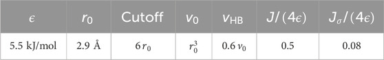
Table 1. The CVF parameters. The parameters for the Lennard-Jones potential modeling the van der Waal interaction, $ϵ$ and $r_0$, are adopted as units of energy and length, respectively.

Both experimental and computational studies indicate that bulk water molecules form four tetrahedral HBs in their lowest energy state. Excited states correspond to defects in the HB network, where molecules have either fewer or more HBs. Ab initio calculations for liquid water at ambient conditions show that under-coordinated molecules comprise approximately 45% of the HB network, while over-coordinated molecules account for less than 5% (DiStasio et al., 2014). According to neutron scattering and Raman spectroscopy studies (Giguère, 1987), bifurcated hydrogen bonds—where one acceptor interacts with two donors—could potentially enable the formation of up to five HBs. However, the energy of each bifurcated HB is approximately half that of a canonical HB. The current consensus suggests that molecules can rapidly switch their HBs between two neighboring molecules within their coordination shell, within hundreds of femtoseconds (Laage and Hynes, 2006). This dynamics, which resembles, on average, a bifurcated HB, is included in our model. Therefore, to simplify, we impose a maximum of four HBs per molecule, introducing variables ${\eta }_{ij}$, which are set to 1 or 0 depending on whether the HB between molecules $i$ and $j$ is allowed, as described in Supplementary Material: Checkerboard partition for $\eta$ variables.

Finally, the enthalpy of the system is given by:

$H\left(N,P,T\right)=U_{\text{LJ}}-N_{\text{HB}}J-N_{\sigma }{J}_{\sigma }+PV,(4)$

where $U_{\text{LJ}}$ is the Lennard-Jones potential in Equation 1 $U_{\text{LJ}}$(r), $N_{\text{HB}}\equiv {\sum }_{⟨i,j⟩}\theta (r_{1/2}-r_{i,j})\delta ({\sigma }_{i,j},{\sigma }_{j,i}){\eta }_{i,j}$, $N_{\sigma }\equiv {\sum }_k^N{\sum }_{⟨i,j⟩}\delta ({\sigma }_{k,j},{\sigma }_{k,i})$, and $V$ is given by Equation 2. Here, $r_{i,j}\equiv |\overrightarrow{r_i}-\overrightarrow{r_j}|$ is the distance between molecules $i$ and $j$, and $\theta (r)$ and $\delta (i,j)$ are the Heaviside step and Kronecker delta functions, respectively. Thus, the formation of a macroscopic HB network leads to an increase in volume for Equation 2, a decrease in entropy due to the reduced number of accessible ${\sigma }_{ij}$ states, and an increase in HB enthalpy, for Equation 4.

2.2 Monte Carlo step definition

A configuration of the CVF model is defined by the variables $\{\overrightarrow{r_i},{\sigma }_{ij},{\eta }_{ij}\}$. In the present version of the model, as discussed above, we coarse-grain the molecule position $\overrightarrow{r_i}$ over the lattice cell and assign to each molecule a proper volume $v_i$, Equation 3. Therefore, considering the definitions of $V_{\text{iso}}$ and ${\eta }_{ij}$, the CVF configuration of the present model reduces to $\{V_{\text{iso}},{\sigma }_{ij},{\eta }_{ij}\}$.

In each MC step, we update these variables in the following order:

1. Update $V_{\text{iso}}$, keeping $\{{\sigma }_{ij},{\eta }_{ij}\}$ fixed.

2. Update ${\eta }_{ij}$, keeping $\{V_{\text{iso}},{\sigma }_{ij}\}$ fixed.

3. Update ${\sigma }_{ij}$, keeping $\{V_{\text{iso}},{\eta }_{ij}\}$ fixed.

We use the standard Metropolis algorithm to update the global variable $V_{\text{iso}}$. This method involves accepting or rejecting a tentative change from $V_{\text{iso}}$ to $V_{\text{iso}}+\mathrm{\Delta }{V}_{\text{iso}}$ with a probability proportional to $\exp [-P\mathrm{\Delta }{V}_{\text{iso}}/(k_{B}T)]$, where $\pm \mathrm{\Delta }{V}_{\text{iso}}\propto \mathcal{O}(V_{\text{iso}}/100)$. We update the ${\eta }_{ij}$ as described in Supplementary Material: Checkerboard partition for $\eta$ variables. For the ${\sigma }_{ij}$, we employ the parallel local Metropolis algorithm (Section 2.3) or the parallel Swendsen-Wang cluster algorithm (Section 2.4), depending on the temperature: Metropolis for $T\ge 208$ K and Swendsen-Wang for lower temperatures.

2.3 Metropolis

The Metropolis algorithm on a regular lattice can be efficiently parallelized by dividing the space into domains for simultaneous variable updates. To maintain detailed balance, the enthalpy change from altering a variable must remain independent of other variables within the same domain. For the Ising model, common partitioning schemes include layered (Barkema and MacFarland, 1994) and checkerboard (Heermann and Burkitt, 1990) methods, with CUDA implementations available for both 2D and 3D (Hawick et al., 2011; Weigel and Yavorskii, 2011; Wojtkiewicz and Kalinowski, 2015). However, these methods are not easily applicable to the CVF model due to differing lattice topologies, so we use a layered partition that enables memory coalescing in the CVF model.

We partition the $\{{\sigma }_{ij}\}$ variables, as described in Figure 1 (Top), into six domains. Each domain contains variables interacting with six bonding indices: five on the same molecule and one on a n.n. Molecule, all from different domains. Therefore, we can update all the ${\sigma }_{ij}$ in the same domain simultaneously.

Figure 1

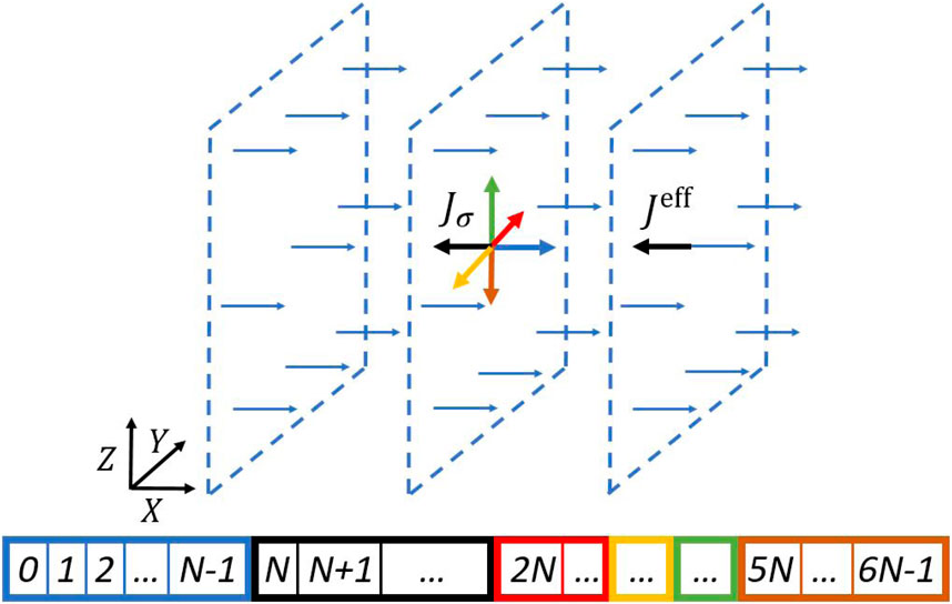
Figure 1. Schematic illustration of the layered domains partitioning the bonding indices $\{{\sigma }_{ij}\}$. (Top) Three layers (marked by dashed lines) of water molecules along the direction $x$. If $i$ is the central molecule, the colored arrows represent the bonding indices $\{{\sigma }_{ij}\}$ where $j$ runs over the n.n. molecules. The bonding index’s color code with the n.n. molecule is blue for the right molecule, black for the left molecule, red for the back molecule, yellow for the front molecule, green for the top molecule, and brown for the bottom molecule. For clarity, we indicate only the blue arrow for the other molecules in the figure. The set $\{{\sigma }_{ij}\}$ is divided into six domains, one for each color. Therefore, the blue domain, represented in the figure, includes all the ${\sigma }_{ij}$ where $x_j=x_i+{(v_{\text{iso}}/v_0)}^{1/d}$. The blue variable ${\sigma }_{ij}$ interacts with the five (different colors, same molecule) ${\sigma }_{ik}$ with $k\ne j$ via the cooperative interaction with characteristic energy $J_{\sigma }$, and, if ${\eta }_{ij}=1$, with the black variable ${\sigma }_{ji}$ via the characteristic energy $J^{\text{eff}}\equiv J-P{v}_{HB}$. (Bottom) Array sorting of the ${\eta }_{ij}$ and ${\sigma }_{ij}$ variables, according to the indexing formula described in the text, grouped by the color-coded domains. The ordering is relevant since it enables coalesced reading, improving the performance.

In CUDA applications, the main bottleneck in execution arises from data access latency (Tapia and D’Souza, 2011). Performance can be enhanced by efficiently sorting memory to exploit memory coalescing (Leist et al., 2009; Sanders and Kandrot, 2010; NVIDIA, 2022). The GPU creates, manages, schedules, and executes blocks of 32 threads simultaneously, called warps (Hawick et al., 2011). When a kernel reads (or writes) to global memory locations, it performs a single coalesced read (or write) transaction for every half-warp of 16 threads. Therefore, we are interested in sorting the vectors so that consecutive threads read (or write) consecutive memory addresses.

We achieve this by sorting the arrays that store ${\eta }_{ij}$ and ${\sigma }_{ij}$ variables according to the index $\mathtt{i}\mathtt{d}\mathtt{x}=\mathtt{a}\mathtt{r}\mathtt{m}\cdot N+\mathtt{c}\mathtt{e}\mathtt{l}\mathtt{l}$, where $\mathtt{a}\mathtt{r}\mathtt{m}\in \{\mathrm{0,1},\dots ,5\}$, and $\mathtt{c}\mathtt{e}\mathtt{l}\mathtt{l}\in \{\mathrm{0,1},\dots ,N-1\}$. The index $\mathtt{a}\mathtt{r}\mathtt{m}$ represents the six possible neighbors of the cell (from 0 to 5: left, right, front, back, top, bottom), and $\mathtt{c}\mathtt{e}\mathtt{l}\mathtt{l}\equiv i$ is the index of the cell (Figure 1 Bottom).

We implement a CUDA kernel gpu_metropolis(arm) that launches one thread per water molecule $i$, where $\mathtt{a}\mathtt{r}\mathtt{m}$ indicates which of the six independent domains is updated (Supplementary Algorithm 1). We define a parallel Metropolis update as six sequential calls to gpu_mertopolis(arm), where arm is chosen randomly to mimic the random selection of ${\sigma }_{ij}$ variables in the sequential Metropolis and to avoid the propagation of correlation waves.

We illustrate how the kernel gpu_metropolis(arm) performs coalesced memory transactions with the following example. We consider a half-warp that updates the block $\mathtt{d}\mathtt{i}\mathtt{r}=0$ (left domain) of the water cells $\mathtt{c}\mathtt{e}\mathtt{l}\mathtt{l}\in \{0,\dots ,15\}$. Thus, idx takes values from 0 to 15. When the kernel estimates $\mathrm{\Delta }{N}_{\text{HB}}$, it reads the right arms of the neighboring cells 1 to 16, i.e., the (consecutive) positions idx $=65$ to 80. The same occurs when estimating $\mathrm{\Delta }{N}_{\sigma }$, as the kernel reads memory positions in consecutive domains. We observe that an exception to this rule arises when the neighboring cell is positioned on the opposite side of the simulation box due to the periodic boundary conditions.

2.4 Swendsen-Wang

Local MC algorithms, such as Metropolis, experience a critical slowdown in their dynamics as the correlation length approaches the system size (as discussed in Section 3.1). In contrast, cluster MC algorithms efficiently update entire correlated regions of spins (clusters) simultaneously. Consequently, they produce statistically independent configurations at significantly lower computational costs. This efficiency is crucial in the supercooled region, for example, where the model exhibits a liquid-liquid phase transition culminating in a liquid-liquid critical point (Coronas and Franzese, 2024). In this context, we examine the Swendsen-Wang (SW) multi-cluster algorithm (Swendsen and Wang, 1987). The algorithm is defined so that, at each step, clusters of ${\sigma }_{ij}$ variables are formed with sizes ranging from 1 (an isolated ${\sigma }_{ij}$ variable) to the system’s size $N$. This formation follows a distribution that reproduces that of thermodynamically correlated degrees of freedom, as discussed in detail in (Bianco and Franzese, 2019) based on site-bond correlated percolation (Kasteleyn and Fortuin, 1969; Coniglio et al., 1979). The new configuration is generated by updating all the (correlated) ${\sigma }_{ij}$ variables within the same cluster to a new state. The sequential SW algorithm for the CVF model proceeds as follows:

1. Visit all the cells $i$. For each $i$, loop over all the pairs of variables $({\sigma }_{ij},{\sigma }_{ik})$. If they are in the same state, place a fictitious bond between them with probability $p_{\sigma }=1-\exp \left(-J_{\sigma }/k_{B}T\right)$.

2. Visit all the pairs of n.n. Cells $⟨i,j⟩$. If $J^{\text{eff}}\equiv J-P{v}_{HB}>0$, ${\eta }_{ij}=1$, and ${\delta }_{{\sigma }_{ij},{\sigma }_{j,i}}=1$, place a fictitious bond with probability $p_{\text{eff}}=1-\exp \left(-\left|J^{\text{eff}}\right|/k_{B}T\right)$. Instead, if $J^{\text{eff}}<0$, place a fictitious bond with probability $p_{\text{eff}}$ if ${\delta }_{{\sigma }_{ij},{\sigma }_{ji}}=0$.

3. Use the Hoshen-Kopelman algorithm (Hoshen and Kopelman, 1976) to identify the clusters of ${\sigma }_{ij}$ variables connected by fictitious bonds.

4. Visit all the clusters. For each, choose a random integer $\mathtt{r}\mathtt{n}\mathtt{d}\text{\_}\text{int}\in \{0,\dots ,q-1\}$. Change the state of all the ${\sigma }_{ij}$ variables in the cluster to ${\sigma }_{ij}\leftarrow \left({\sigma }_{ij}+\mathtt{r}\mathtt{n}\mathtt{d}\text{\_}\text{int}\right)\%q$, where $\leftarrow$ is the assignment operator and $\%$ is the modulo operation.

The SW algorithm performs three independent tasks. First, it places fictitious bonds between ${\sigma }_{ij}$ variables to generate the clusters. Second, it identifies all the clusters. Third, it updates each cluster. The first and third tasks are highly localized and can be easily parallelized. However, this is not the case for the cluster labeling operation. To tackle this challenge, we build on the work of Hawick et al., who developed various parallel labeling algorithms for arbitrary and lattice graphs using CUDA (Hawick et al., 2010). Among these, the label equivalence algorithm was refined by Kalentev et al. (Kalentev et al., 2011) and later applied by Komura and Okabe to SW simulations of the 2D Potts model (Komura and Okabe, 2012). In this context, we modify the Hawick-Kalentev label-equivalence algorithm for the CVF model.

For a given SW step, we first generate the clusters. We directly parallelize this task so that each thread works on one CVF cell. Each thread is responsible for the cooperative interactions within its cell and the covalent interactions with the left, front, and top directions. To accomplish this, we allocate the array connected of size $(15+3)N=18N$, which indicates whether two neighboring ${\sigma }_{ij}$ variables belong to the same cluster. We nest this array based on the index $\mathtt{c}\mathtt{o}\mathtt{n}\text{\_}\mathtt{i}\mathtt{d}\mathtt{x}=\mathtt{l}\mathtt{i}\mathtt{n}\mathtt{k}N+\mathtt{c}\mathtt{e}\mathtt{l}\mathtt{l}$, where $\mathtt{l}\mathtt{i}\mathtt{n}\mathtt{k}\in \{0,\dots ,17\}$. $\mathtt{l}\mathtt{i}\mathtt{n}\mathtt{k}=0$, 1, and 2 represents the covalent connections between cell and its neighbors in the left, front, and top directions. The values $\mathtt{l}\mathtt{i}\mathtt{n}\mathtt{k}\in \{3,\dots ,17\}$ represent the 15 cooperative connections within $\mathtt{c}\mathtt{e}\mathtt{l}\mathtt{l}$.

Once the bonds are placed, we apply the label equivalence algorithm. We allocate the $\mathtt{l}\mathtt{a}\mathtt{b}\mathtt{e}\mathtt{l}$ array of size $6N$, which indicates the cluster that ${\sigma }_{ij}$ belongs to. Thanks to Kalentev’s sophistication, this array also resolves label equivalences (Kalentev et al., 2011). The advantage is the reduction of the memory cost of the algorithm, which is significant due to the limited storage resources of the GPUs. We initialize $\mathtt{l}\mathtt{a}\mathtt{b}\mathtt{e}\mathtt{l}$ as $\mathtt{l}\mathtt{a}\mathtt{b}\mathtt{e}\mathtt{l}[\mathtt{i}\mathtt{d}\mathtt{x}]=\mathtt{i}\mathtt{d}\mathtt{x}$, where $\mathtt{i}\mathtt{d}\mathtt{x}$ is the ${\sigma }_{ij}$ index defined in Metropolis. The algorithm resolves label equivalences through iterative calls to the scanning and analysis functions (Kalentev et al., 2011; Komura and Okabe, 2012). When the algorithm converges, all the ${\sigma }_{ij}$ variables in the same cluster will take the same $\mathtt{l}\mathtt{a}\mathtt{b}\mathtt{e}\mathtt{l}$ value.

The scanning function compares the label of a site $\mathtt{i}\mathtt{d}\mathtt{x}$ to the labels of all the n.n. ${\sigma }_{ij}$ within the cluster. For every $\mathtt{i}\mathtt{d}\mathtt{x}$, label$[\mathtt{i}\mathtt{d}\mathtt{x}]$ is updated to the minimum value among all the labels of the bonded sites, including itself. In Ref. (Komura and Okabe, 2012), Komura and Okabe implemented this function using a single kernel for the 2D Potts model. However, for the CVF model, we find it more convenient to divide this function into two kernels. First, in gpu_scanning_covalent, each thread scans left, front, and top covalent interactions (Supplementary Algorithm 2). Second, gpu_scanning_cooperative scans the cooperative interactions (Supplementary Algorithm 3). An alternative implementation in a single kernel leads to race conditions when two threads attempt to update the same element of label¹.

Next, the analysis function updates label$[\mathtt{i}\mathtt{d}\mathtt{x}]$ (Supplementary Algorithm 4). This step further propagates the minimum value of label to other ${\sigma }_{ij}$ variables within the same cluster. Although the parallel implementation of the analysis function experiences race conditions, these collisions between threads will eventually be resolved in subsequent applications of the scanning and analysis functions (Kalentev et al., 2011). To minimize the impact of thread conflicts, we implement the gpu_analysis$(\mathtt{a}\mathtt{r}\mathtt{m})$ kernel, which updates only the label of those ${\sigma }_{ij}$ variables in the $\mathtt{a}\mathtt{r}\mathtt{m}$ domain. We then loop through the six domains to account for all the lattice sites.

To check whether the algorithm has converged, we first store a copy of the label vector before calling the scanning and analysis functions, and then we compare it to the updated label. We parallelize this task by assigning one thread to each CVF cell. The algorithm converges when the $\mathtt{l}\mathtt{a}\mathtt{b}\mathtt{e}\mathtt{l}$ remains unchanged. We provide an example of label convergence after successive applications of the scanning and analysis functions in Table 2.

Table 2

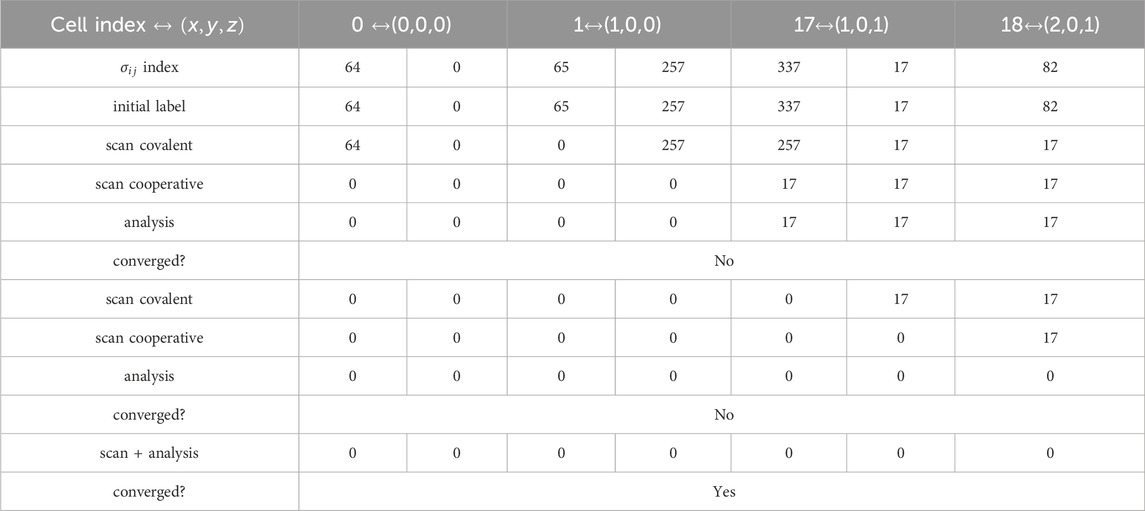
Table 2. Example of parallel label equivalence algorithm. We consider a small cluster of seven ${\sigma }_{ij}$ variables with indices in “${\sigma }_{ij}$ index” row in a lattice of $N=64$ cells. Each pair of ${\sigma }_{ij}$ variables in the same cell (cell index $\leftrightarrow$ Cartesian coordinates row) are bonded through a cooperative interaction. The pairs of ${\sigma }_{ij}$ variables (0,65), (257,337), and (17,82) are bonded through a covalent interaction. The initial value of label coincides with the ${\sigma }_{ij}$ index. The following lines show the resulting label after the application of the kernels scan covalent, scan cooperative, and analysis. At the third iteration, label does not change, so this cluster has converged. The SW step ends when all the clusters converge.

3 Results and discussion

3.1 Critical slowdown of the metropolis dynamics in the vicinity of the liquid-liquid critical point

The CVF model predicts a liquid-liquid phase transition (LLPT) between high-density liquid (HDL) and low-density liquid (LDL) phases in the supercooled region (Coronas and Franzese, 2024). The LLPT ends in a liquid-liquid critical point (LLCP), located at $P_C=$ 174 $\pm$ 14 MPa and $T_C=$ 186 $\pm$ 4 K in the thermodynamic limit $(N\to \infty )$. This is in close agreement with finite-$N$ estimates from iAMOEBA (Pathak et al., 2016), TIP4P/Ice (Debenedetti et al., 2020), and ML-BOP (Dhabal et al., 2024) models, as well as with a recent estimate from a collection of experimental data (Mallamace and Mallamace, 2024).

Approaching the LLCP, the correlation length $\xi$ of the water HB network increases and ultimately diverges at the critical point. Consequently, the autocorrelation time $\tau$ of the local Metropolis MC dynamics, which is proportional to $\xi$, also increases approaching the LLCP. This can be demonstrated by calculating the autocorrelation function

$C_M\left(\mathrm{\Delta }t\right)\equiv \frac{\langle M_i\left(t_0+\mathrm{\Delta }t\right)M\left(t_0\right)\rangle -{\langle M\rangle }^2}{\langle M^2\rangle -{\langle M\rangle }^2},(5)$

where $M\equiv \frac{1}{qN}\max \{N_{q^{\prime }}\}$ is an order parameter, and $N_{q^{\prime }}$ is the number of ${\sigma }_{ij}$ variables in the state $q^{\prime }\in \{0,\dots ,q-1\}$. We define the autocorrelation time $\tau$ as the time at which $C(\tau )=1/e$. Thus, $C(\mathrm{\Delta }t)$ allows us to estimate the autocorrelation time $\tau$ of the HB network. Two CVF configurations are uncorrelated if they are sampled after a number of MC steps $\ge \tau$.

We calculate, with the Metropolis algorithm, $C_M(\mathrm{\Delta }t)$ for a system with $N=32768$ water molecules (Figure 2a). At a pressure of $P=160$ MPa, which is close to the critical pressure in the thermodynamic limit ($P=174\pm 14$ MPa), $\tau$ displays non-monotonic behavior with fast dynamics at high $T=208$ K and low $T=188$ K, alongside an apparent divergence at $T=193$ K. This behavior is linked to a structural change between HDL-like and LDL-like forms of water, characterized by the Widom line (the locus of maxima of $\xi$) emerging from the LLCP at higher pressure (Coronas and Franzese, 2024). As an approximate estimate of the Widom line, we present the locus of extrema of the specific heat $C_P$, namely, the maxima of the enthalpy fluctuations (Figure 2b). At extremely low pressure, $P=-300$ MPa, far from the critical region, $\tau$ exhibits a similar non-monotonic behavior, but without any apparent divergence upon crossing the Widom line. This is consistent with a decrease in the maxima of the correlation length $\xi$ as the distance between the LLCP and the point along the Widom line increases.

Figure 2

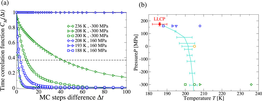
Figure 2. (a) Correlation function ${\mathit{C}}_{\mathit{M}}(\mathrm{\Delta }\mathit{t})$ of the order parameter $\mathit{M}$ for parallel Metropolis MC algorithm. The time $\mathrm{\Delta }t$ is measured in units of MC steps. The system size is $N=32768$. At $P=$160 MPa and $T=$193 K (blue triangles), near the estimate of the supercooled water LLCP in the thermodynamic limit (Coronas and Franzese, 2024), the correlation function decreases very slowly, consistent with the critical slowing down expected for local MC dynamics near a critical point. As temperature increases ($T=208$ K, blue diamonds) or decreases ($T=188$ K, blue squares) at constant pressure, the correlation decays more rapidly. A similar trend is observed at low-$P=-300$ MPa, with slow decay at $T=208$ K (green triangles) and faster decay at higher $T=236$ K (green diamonds) and lower $T=200$ K (green squares). The dashed line indicates the $C_M=e^{-1}$ value corresponding to the autocorrelation time $\tau$. (b) Location of simulated thermodynamic points in the $\mathit{P}$-$\mathit{T}$ phase diagram. From the LLCP (red), the locus of extrema of the correlation length $\xi$, i.e., the Widom line, emerges. As a proxy estimate of the Widom line, we plot the locus of maxima of the specific heat, i.e., the maxima of enthalpy fluctuations (turquoise line) as discussed in (Coronas and Franzese, 2024). The blue and green symbols correspond to the thermodynamic conditions selected in panel (a) and Figure 3.

3.2 Cluster MC dynamics avoids the critical slowdown

Cluster MC algorithms are suitable for efficiently sampling the critical region, as they bypass the critical slowdown of the dynamics by updating regions of correlated HBs simultaneously. We compare the autocorrelation function (Equation 5) computed with local Metropolis (Figure 3a) and cluster SW (Figure 3b) algorithms. As discussed in Section 3.1, we observe slow dynamics of the system at low $P=-300$ MPa and $T=205$ K, near the Widom line. With increasing pressure ($P=0.1$ MPa) at constant temperature, the system remains in a metastable supercooled liquid state, exhibiting rapid decorrelation. Finally, at $T=195$ K and $P=160$ MPa, close to the LLCP (174 $\pm$ 14 MPa, 186 $\pm$ 4 K) (Coronas and Franzese, 2024), the autocorrelation time appears to diverge. The comparison with SW illustrates that cluster MC circumvents the critical slowdown of the dynamics in all cases, even near the LLCP.

Figure 3

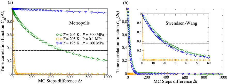
Figure 3. Comparison between correlation function ${\mathit{C}}_{\mathit{M}}(\mathrm{\Delta }\mathit{t})$ computed with Metropolis and SW. (a) For the Metropolis MC, at $P=$160 MPa and $T=$195 K (blue triangles), near the LLCP, the correlation function decreases very slowly, as discussed in Figure 2. At a higher temperature of $T=205$ K and a lower pressure of $P=-300$ MPa (green circles) near the Widom line, the correlation function exhibits a slow decay. Away from the Widom line, at the same temperature but at a higher pressure of $P=0.1$ MPa (orange circles), the correlation function decays much faster. (b) The SW algorithm avoids the critical slowdown of dynamics at the same state points (symbols and colors as in panel a). Inset: An enlarged view of the short-time regime enhances the distinction among the data for different state points.

Caution should be taken for the interpretation of time autocorrelation functions computed through MC simulations. Molecular Dynamics (MD) and MC fundamentally differ in how they explore the configurational phase space. While MD solves the time evolution of the system, MC proposes random updates of the system that are accepted or rejected with a probability given by the Boltzmann factor. Consequently, the MC timestep does not have a direct physical meaning. It is a computational step used to explore the configuration space, but it does not correspond to any real elapsed time. If MD is used, time correlation functions are a physical property of the system and describe how quickly a property, such as the HB lifetime, decorrelates. Conversely, when employing MC, time correlation functions reflect the algorithm’s ability to propose (and accept) configurations that vary with respect to a specific property. In the MC context, the time correlation function is not a property of the system but a property of the algorithm. Indeed, Metropolis and SW algorithms explore the same free energy landscape with identical equilibrium configurations; however, they differ in the number of steps needed to reach other equilibrium microstates. Hence, differences in MC time autocorrelation functions between Metropolis and SW do not reflect different physical properties of the simulated system but rather different algorithm efficiencies.

3.3 Benchmark of the algorithms

As discussed above, the autocorrelation time $\tau$ for the SW algorithm is significantly shorter than that for the Metropolis MC. However, SW cluster MC is notably more computationally expensive than Metropolis. Therefore, to determine which MC dynamics is more efficient in generating uncorrelated configurations, one must compare the time each algorithm takes to produce $\tau$ MC steps.

First, we analyze the computational cost of the parallel Metropolis algorithm for different system sizes, $N\le 17576000$. The hardware and software specifications of the workstation are detailed in Supplementary Material: Workstation. Depending on the system size, we perform between 2 and 10 independent simulations of $5000$ MC steps. We find that the results are robust against changes in thermodynamic conditions; that is, changes in $T$ and $P$ do not affect the computational cost of the algorithm (Supplementary Algorithm 1).

Our results show that the time necessary (cost) for a parallel Metropolis update scales linearly for $32768\le N\le 2097152$ (Figure 4). For these systems, the GPU resources are neither saturated (large $N$) nor under-exploited (small $N$); thus, the time spent on data accessing scales linearly with $N$. For small $N\le 8000$, the computational resources of the GPU are not optimized. We find that in this range, the time cost of a Metropolis step remains approximately constant ($\sim 0.1$ ms, Figure 4: inset). For large $N\ge 2097152$, the size of the arrays of random numbers must be reduced to fit within the GPU global memory (Supplementary Material: Generation and usage of random numbers). The additional time cost arises from both the increasing number of executions of the kernels for generating random numbers and the time involved in memory transactions. In particular, we benchmark accessible size-systems up to $N=17576000$ water molecules with a time cost of 280 m per Metropolis update (Figure 4), which corresponds to a cubic simulation box of $75\times 75$ $\times$ 75 ${\text{nm}}^3$.

Figure 4

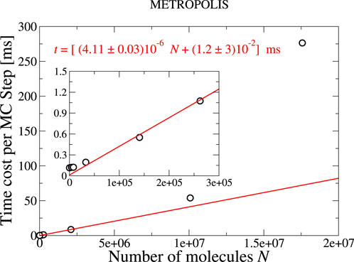
Figure 4. Time cost of a parallel Metropolis update of 64 $\le \mathit{N}\le$ 17,576 000 water molecules. The line is a linear fit $t=aN+b$ of the time cost within the range $32768\le N\le 2097152$, with fitting parameters $a=(4.11\pm 0.03)10^{-6}$ ms and $b=(1.2\pm 3)10^{-2}$ ms. We observe a large deviation from linearity for $N>10^7$. Inset: The enlarged view at small $N$ highlights the deviation from linearity for $N\le 8000$, with a time cost saturation $\sim 0.1$ ms at small $N$. In both the main panel and the inset, error bars are smaller than the size of the symbols.

We estimate the size-dependent performance gain, or speedup factor, SF$(N)\equiv t^{\text{CPU}}/t^{\text{GPU}}$, defined as the ratio between the time required for a parallel and a sequential update of an entire system of $N$ molecules, as shown in Table 3. The results indicate that, for the smallest system considered ($N=64$ molecules), the parallel algorithm is less efficient than the sequential one. This is not surprising, as a sufficiently large number of threads must be executed to fully utilize the GPU resources (Hall et al., 2014). Indeed, Wojtkiewicz and Kalinowski also find $\mathrm{S}\mathrm{F}<1$ for small systems (Wojtkiewicz and Kalinowski, 2015). The large SF$=136.72$ measured for $N=2097152$ is attributed to the significant increase in the time cost of the sequential implementation compared to the parallel approach. More specifically, we find that the large $\sigma$ and $\eta$ arrays exceed the RAM storage capacity, necessitating that they be loaded in portions, which delays the sequential computation. We could not measure the SF for $2097152<N\le 17576000$ due to the excessive cost of computing $t^{\text{CPU}}$. Instead, we extrapolated SF$=208$ for $N=10077696$ and SF$=245.8$ for $N=17576000$ from a power-law fit in the range $32768\le N\le 2097152$ (see Supplementary Figure S3). Further details on the computation of the SF are provided in Supplementary Material: Speedup factors.

Table 3

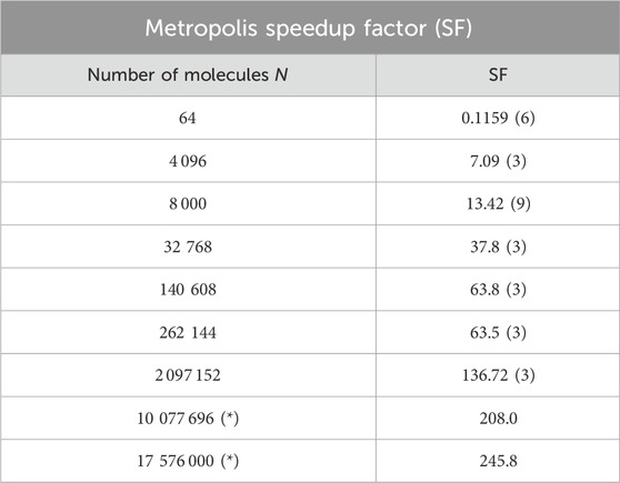
Table 3. Speedup factor, SF$\equiv t^{\text{CPU}}/t^{\text{GPU}}$, of the GPU Metropolis algorithm in comparison to the sequential implementation on the CPU for $N$ water molecules. The error in the last digit of the estimate is indicated in parentheses. (*) For N ≥ 10 077 696, we extrapolate SF from a power law fit (Supplementary Figure S3).

Next, we estimate the performance of the parallel SW algorithm. Unlike the Metropolis case, the time cost of a SW update depends on the cluster size distribution, which in turn is influenced by the thermodynamic conditions (Bianco and Franzese, 2019). Close to the Widom line, the system undergoes a transition from non-percolation to percolation upon isobaric cooling. Thus, we consider two temperatures on either side of the transition: $T=$ 195 K (percolation) and 210 K (not percolation), with $P=0.1$ MPa. For every system size $N$, we perform between 5 and 10 independent simulations of $10^3$ MC steps.

We find that the time cost of the parallel SW algorithm increases linearly for $N\le \mathrm{262,144}$, although data at small values of $N$ are noisy (Figure 5). As with the parallel Metropolis algorithm, we attribute this to the suboptimal usage of GPU resources.

Figure 5

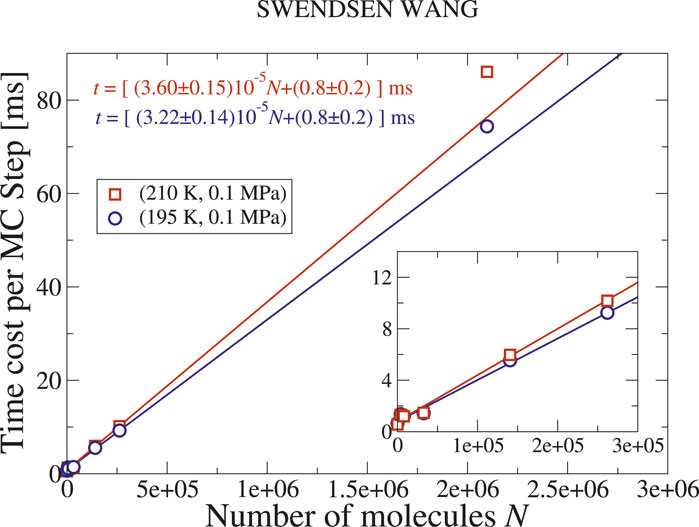
Figure 5. Time cost of a parallel SW cluster update of $\mathit{N}$ water molecules. Red squares correspond to $T=$ 210 K (non-percolating cluster) and blue circles correspond to $T=195$ K (percolating cluster) at pressure $P=0.1$ MPa. Lines with matching colors indicate linear fits of the data, expressed as $t=aN+b$, within the range $16\le N\le 2097152$. The fitting parameters Are $a=(3.60\pm 0.15)\times 10^{-5}$ ms and $b=(0.8\pm 0.2)$ ms for the red line, and $a=(3.22\pm 0.14)\times 10^{-5}$ ms and $b=(0.8\pm 0.2)$ ms for the blue line, respectively. We observe that the cost increases faster than linear at large $N$ and exceeds that of the Metropolis MC, limiting our ability to explore sizes with tens of millions of water molecules, which contrasts with the Metropolis case. Inset: The enlarged view at small $N$ highlights excellent linearity for the small $N$. In both the main panel and the inset, error bars are smaller than the size of the symbols.

At larger values of $N$, we observe additional time costs compared to linearity. As in the Metropolis case, we attribute this to limited resources for storing large arrays, such as those used for random numbers. However, the cost value reached at $N=2097152$ for SW is approximately 1.6 times larger than in the Metropolis case for the same size, which limits our ability to explore sizes with tens of millions of water molecules.

We note that the parallel SW update is faster under percolating conditions than in the absence of percolation. Although a better performance for a cluster algorithm is expected when the correlation length is large, because larger clusters lead to fewer in number, this result is not obvious. One might expect that the total time cost of the update is governed by the time cost of labeling the largest cluster, as seen in the sequential implementation.

A possible explanation is that the analysis function converges rapidly irrespective of the cluster size, making the size of the largest cluster less relevant. Therefore, the difference in time cost between percolation and non-percolation likely stems from less efficient memory readings of the label array in smaller clusters by the scanning and labeling functions.

A further consequence of this feature of the parallel implementation on GPUs is that the speedup factor relative to the sequential implementation on CPUs is greater under percolation conditions (Table 4; Supplementary Figure S4). In particular, we find that for $N\ge 32768$, the SF under percolating conditions is nearly twice that under non-percolating conditions.

Table 4

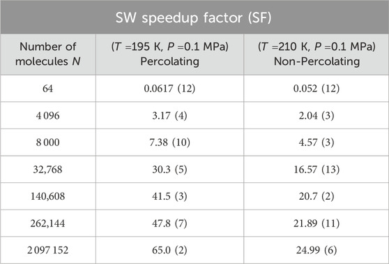
Table 4. As in Table 3, but for the GPU Swendsen-Wang algorithm under the two thermodynamic conditions shown in Figure 5.

Based on our results, we observe that the time cost of a single MC update for a CVF water sample of $N=32768$ molecules (as discussed in Sections 3.1, 3.2) is 0.15 m using Metropolis. In the case of SW, the time cost is 1.9 m for percolating clusters, i.e., approaching the LLCP, and 2.0 m for non-percolating clusters, away from the critical region.

Therefore, the SW algorithm is approximately ten times more costly than Metropolis for $N=32768$. This result suggests that the SW algorithm should be employed whenever the autocorrelation time $\tau$ obtained with SW is at least ten times shorter than the $\tau$ obtained with Metropolis. As we have discussed above, this occurs when the system approaches the Widom line (the maximum of the correlation length $\xi$) or the region of maxima of specific heat (the maximum of enthalpy fluctuations).

4 Conclusion

In this work, we implement efficient parallel MC algorithms for the CVF model of bulk water. In particular, we design a Metropolis algorithm based on a layered partition scheme and adapt the label equivalence algorithm from Hawick et al. (2010) and Kalentev et al. (2011) for simulations using the SW algorithm. Our results show that when the correlation length of the HB network is small, the parallel Metropolis algorithm is more efficient than the SW. This efficiency arises because the Metropolis algorithm takes less time per update to perform memory and computation tasks. Specifically, we demonstrate that a single Metropolis update is roughly ten times faster than an update with the SW algorithm for $N=32768$.

However, the Metropolis dynamics suffer from slowing down when the correlation length $\xi$ of the HB network is large. This occurs when the thermodynamic conditions are close to the Widom line, for example, at ambient pressure and supercooled conditions, $T\lesssim 205$ K, or near the LLCP (174 $\pm$ 14 MPa, 186 $\pm$ 4 K) (Coronas and Franzese, 2024) where $\xi$ eventually diverges. Thanks to simultaneous updates of correlated clusters, the SW algorithm avoids the critical slowing down of the dynamics, enabling efficient sampling under those conditions. Therefore, we conclude that the SW algorithm should be preferred when the system is near a critical point or the corresponding Widom line, as the increased computational time for a single update is balanced by the fewer Monte Carlo steps required to yield statistically independent configurations.

Furthermore, we observe that the speedup factor of the GPU implementation, in relation to the CPU implementation, of the 2 MC algorithms can be approximately 137 for Metropolis and 65 for SW when $N=2097152$. Therefore, regardless of the algorithm used, we find that GPU parallelization enables the CVF model to scale for simulations of unprecedentedly large water systems, reaching tens of millions of water molecules.

For instance, we benchmark systems of 17,576 000 water molecules using the Metropolis algorithm, and 2 097 152 molecules for the SW cluster MC. The smaller size for the SW algorithm results from its higher computational cost in terms of time and memory compared to Metropolis dynamics.

Combining these results with the observation that the CVF model is reliable, given its quantitative accuracy around ambient conditions (Coronas et al., 2025), and is transferable at extreme thermodynamic conditions (Coronas and Franzese, 2024), we conclude that the CVF model is suitable for addressing problems in nanotechnology and nanobiology due to its accuracy, efficiency, and scalability. Furthermore, we observe that, although many relevant issues in these scientific areas occur at near-ambient conditions, the model’s transferability at extreme conditions is essential for a better understanding of phenomena such as protein denaturation upon heating, cooling, pressurization, or depressurization (Bianco and Franzese, 2015).

To further support these conclusions, we have demonstrated in preliminary work (Coronas, 2023) that CVF water enables us to calculate the free energy landscape of extensive biological systems that were previously simulatable only with implicit solvents. In particular, we examined the sequestration of superoxide dismutase 1 (SOD1) proteins into crowded bovine serum albumin (BSA) globular protein and Fused in Sarcoma (FUS) disordered protein environments (Samanta et al., 2021), as well as the shear-induced unfolding of the von Willebrand factor (Languin-Cattoën et al., 2021). Both cases were previously analyzed using the OPEP protein model with implicit solvent (Timr et al., 2023).

In conclusion, the CVF represents a REST—reliable, efficient, scalable, and transferable—model for water and hydrated systems. Its innovative approach holds the promise to transform free energy calculations for large-scale nano-bio systems, paving the way for groundbreaking discoveries in the field.

Data availability statement

The code developed in this work, along with instructions for its compilation and usage, is publicly available in https://github.com/lcoronas/CVFBulkWater.

Author contributions

LC: Formal Analysis, Writing – original draft, Validation, Visualization, Data curation, Investigation, Methodology, Software, Writing – review and editing. OV: Methodology, Investigation, Writing – review and editing, Writing – original draft, Software, Formal Analysis. GF: Formal Analysis, Project administration, Writing – original draft, Resources, Data curation, Writing – review and editing, Validation, Conceptualization, Methodology, Supervision, Funding acquisition, Investigation.

Funding

The author(s) declare that financial support was received for the research and/or publication of this article. This work was supported by the Spanish Ministerio de Ciencia e Innovación/Agencia Estatal de Investigación (grant number MCIN/AEI/10.13039/501100011033); the European Commission “ERDF A way of making Europe” (grant number PID2021-124297NB-C31); the Universitat de Barcelona (grant number 5757200 APIF_18_19). GF acknowledges the support from the Ministry of Universities 2023–2024 Mobility Subprogram within the Talent and its Employability Promotion State Program (PEICTI 2021-2023) and the Visitor Program of the Max Planck Institute for The Physics of Complex Systems for supporting a visit started in November 2022.

Acknowledgments

We thank Valentino Bianco and Arne W. Zantop for their contributions to earlier versions of the CVF model.

Conflict of interest

The authors declare that the research was conducted in the absence of any commercial or financial relationships that could be construed as a potential conflict of interest.

Generative AI statement

The author(s) declare that no Generative AI was used in the creation of this manuscript.

Any alternative text (alt text) provided alongside figures in this article has been generated by Frontiers with the support of artificial intelligence and reasonable efforts have been made to ensure accuracy, including review by the authors wherever possible. If you identify any issues, please contact us.

Publisher’s note

All claims expressed in this article are solely those of the authors and do not necessarily represent those of their affiliated organizations, or those of the publisher, the editors and the reviewers. Any product that may be evaluated in this article, or claim that may be made by its manufacturer, is not guaranteed or endorsed by the publisher.

Supplementary material

The Supplementary Material for this article can be found online at: https://www.frontiersin.org/articles/10.3389/fnano.2025.1637828/full#supplementary-material

Footnotes

¹To avoid this, we could use the CUDA atomic_min function; however, we found that it resulted in worse performance due to increased thread divergence (Kalentev et al., 2011).

References

Abella, D., Franzese, G., and Hernández-Rojas, J. (2023). Many-body contributions in water nanoclusters. ACS Nano 17, 1959–1964. doi:10.1021/acsnano.2c06077PubMed Abstract | CrossRef Full Text | Google Scholar

Barkema, G. T., and MacFarland, T. (1994). Parallel simulation of the ising model. Phys. Rev. E 50, 1623–1628. doi:10.1103/PhysRevE.50.1623PubMed Abstract | CrossRef Full Text | Google Scholar

Barnes, P., Finney, J. L., Nicholas, J. D., and Quinn, J. E. (1979). Cooperative effects in simulated water. Nature 282, 459–464. doi:10.1038/282459a0CrossRef Full Text | Google Scholar

Bertolazzo, A. A., and Barbosa, M. C. (2014). Density and diffusion anomalies in a repulsive lattice gas. Phys. Procedia 53, 7–15. doi:10.1016/j.phpro.2014.06.018CrossRef Full Text | Google Scholar

Bianco, V., and Franzese, G. (2014). Critical behavior of a water monolayer under hydrophobic confinement. Sci. Rep. 4, 4440 EP. doi:10.1038/srep04440PubMed Abstract | CrossRef Full Text | Google Scholar

Bianco, V., and Franzese, G. (2015). Contribution of water to pressure and cold denaturation of proteins. Phys. Rev. Lett. 115, 108101. doi:10.1103/physrevlett.115.108101PubMed Abstract | CrossRef Full Text | Google Scholar

Bianco, V., and Franzese, G. (2019). Hydrogen bond correlated percolation in a supercooled water monolayer as a hallmark of the critical region. J. Mol. Liq. 285, 727–739. doi:10.1016/j.molliq.2019.04.090CrossRef Full Text | Google Scholar

Bianco, V., Vilanova, O., and Franzese, G. (2014). “Polyamorphism and polymorphism of a confined water monolayer: liquid-liquid critical point, liquid-crystal and crystal-crystal phase transitions,” in Perspectives and challenges in statistical physics and complex systems for the next decade. Editor M. Viswanathan Gandhimohan, (World Scientific), Singapore: World Scientific Publishing Co. Pte. Ltd. 126–149. doi:10.1142/9789814590143_0008CrossRef Full Text | Google Scholar

Bianco, V., Franzese, G., Dellago, C., and Coluzza, I. (2017a). Role of water in the selection of stable proteins at ambient and extreme thermodynamic conditions. Phys. Rev. X 7, 021047. doi:10.1103/PhysRevX.7.021047CrossRef Full Text | Google Scholar

Bianco, V., Pagès-Gelabert, N., Coluzza, I., and Franzese, G. (2017b). How the stability of a folded protein depends on interfacial water properties and residue-residue interactions. J. Mol. Liq. 245, 129–139. doi:10.1016/j.molliq.2017.08.026CrossRef Full Text | Google Scholar

Bianco, V., Alonso-Navarro, M., Di Silvio, D., Moya, S., Cortajarena, A. L., and Coluzza, I. (2019). Proteins are solitary! pathways of protein folding and aggregation in protein mixtures. J. Phys. Chem. Lett. 10, 4800–4804. doi:10.1021/acs.jpclett.9b01753PubMed Abstract | CrossRef Full Text | Google Scholar

Bianco, V., Franzese, G., and Coluzza, I. (2020). In silico evidence that protein unfolding is a precursor of protein aggregation. ChemPhysChem 21, 377–384. doi:10.1002/cphc.201900904PubMed Abstract | CrossRef Full Text | Google Scholar

Borick, S. S., Debenedetti, P. G., and Sastry, S. (1995). A lattice model of network-forming fluids with orientation-dependent bonding: equilibrium, stability, and implications for the phase behavior of supercooled water. J. Phys. Chem. 99, 3781–3792. doi:10.1021/j100011a054CrossRef Full Text | Google Scholar

Cerdeiriña, C. A., Troncoso, J., González-Salgado, D., Debenedetti, P. G., and Stanley, H. E. (2019). Water’s two-critical-point scenario in the ising paradigm. J. Chem. Phys. 150, 244509. doi:10.1063/1.5096890PubMed Abstract | CrossRef Full Text | Google Scholar

Chan, H., Cherukara, M. J., Narayanan, B., Loeffler, T. D., Benmore, C., Gray, S. K., et al. (2019). Machine learning coarse grained models for water. Nat. Commun. 10, 379. doi:10.1038/s41467-018-08222-6PubMed Abstract | CrossRef Full Text | Google Scholar

Chaplin, M. (2006). Do we underestimate the importance of water in cell biology? Nat. Rev. Mol. Cell Biol. 7, 861–866. doi:10.1038/nrm2021PubMed Abstract | CrossRef Full Text | Google Scholar

Cisneros, G. A., Wikfeldt, K. T., Ojamäe, L., Lu, J., Xu, Y., Torabifard, H., et al. (2016). Modeling molecular interactions in water: from pairwise to many-body potential energy functions. Chem. Rev. 116, 7501–7528. doi:10.1021/acs.chemrev.5b00644PubMed Abstract | CrossRef Full Text | Google Scholar

Cobar, E. A., Horn, P. R., Bergman, R. G., and Head-Gordon, M. (2012). Examination of the hydrogen-bonding networks in small water clusters (n = 2–5, 13, 17) using absolutely localized molecular orbital energy decomposition analysis. Phys. Chem. Chem. Phys. 14, 15328–15339. doi:10.1039/C2CP42522JPubMed Abstract | CrossRef Full Text | Google Scholar

Coniglio, A., Stanley, H. E., and Klein, W. (1979). Site-bond correlated-percolation problem: a statistical mechanical model of polymer gelation. Phys. Rev. Lett. 42, 518–522. doi:10.1103/PhysRevLett.42.518CrossRef Full Text | Google Scholar

Coronas, L. E. (2023). Calculations of water free energy in bulk and large biological systems. Ph.D. thesis, Facultat de Física. Barcelona, Spain: Universitat de Barcelona.

Google Scholar

Coronas, L. E., and Franzese, G. (2024). Phase behavior of metastable water from large-scale simulations of a quantitatively accurate model near ambient conditions: the liquid–liquid critical point. J. Chem. Phys. 161, 164502. doi:10.1063/5.0219313PubMed Abstract | CrossRef Full Text | Google Scholar

Coronas, L. E., Vilanova, O., Bianco, V., de los Santos, F., and Giancarlo, F. (2022). “The Franzese-Stanley coarse grained model for hydration water,” in Water from Numerical and experimental perspectives. 1st ed. (Boca Raton: CRC Press).

Google Scholar

Coronas, L. E., Vilanova, O., and Franzese, G. (2025). A transferable molecular model for accurate thermodynamic studies of water in large-scale systems. J. Mol. Liq. 434, 128032. doi:10.1016/j.molliq.2025.128032CrossRef Full Text | Google Scholar

de Almeida Ribeiro, I., Dhabal, D., Kumar, R., Banik, S., Sankaranarayanan, S. K. R. S., and Molinero, V. (2024). Medium-density amorphous ice unveils shear rate as a new dimension in water’s phase diagram. Proc. Natl. Acad. Sci. 121, e2414444121. doi:10.1073/pnas.2414444121PubMed Abstract | CrossRef Full Text | Google Scholar

de los Santos, F., and Franzese, G. (2011). Understanding diffusion and density anomaly in a coarse-grained model for water confined between hydrophobic walls. J. Phys. Chem. B 115, 14311–14320. doi:10.1021/jp206197tPubMed Abstract | CrossRef Full Text | Google Scholar

de los Santos, F., and Franzese, G. (2012). Relations between the diffusion anomaly and cooperative rearranging regions in a hydrophobically nanoconfined water monolayer. Phys. Rev. E 85, 010602. doi:10.1103/physreve.85.010602PubMed Abstract | CrossRef Full Text | Google Scholar

Debenedetti, P. G., Sciortino, F., and Zerze, G. H. (2020). Second critical point in two realistic models of water. Science 369, 289–292. doi:10.1126/science.abb9796PubMed Abstract | CrossRef Full Text | Google Scholar

Dhabal, D., Kumar, R., and Molinero, V. (2024). Liquid–liquid transition and ice crystallization in a machine-learned coarse-grained water model. Proc. Natl. Acad. Sci. 121, e2322853121. doi:10.1073/pnas.2322853121PubMed Abstract | CrossRef Full Text | Google Scholar

DiStasio, R. A., Santra, B., Li, Z., Wu, X., and Car, R. (2014). The individual and collective effects of exact exchange and dispersion interactions on the ab initio structure of liquid water. J. Chem. Phys. 141, 084502. doi:10.1063/1.4893377PubMed Abstract | CrossRef Full Text | Google Scholar

Durà-Faulí, B., Bianco, V., and Franzese, G. (2023). Hydrophobic homopolymer’s coil–globule transition and adsorption onto a hydrophobic surface under different conditions. J. Phys. Chem. B 127, 5541–5552. doi:10.1021/acs.jpcb.3c00937PubMed Abstract | CrossRef Full Text | Google Scholar

Dutta, S., Lee, Y., and Jho, Y. S. (2015). Hydration of ions in two-dimensional water. Phys. Rev. E 92, 042152. doi:10.1103/PhysRevE.92.042152PubMed Abstract | CrossRef Full Text | Google Scholar

Finney, J. L. (2001). The water molecule and its interactions: the interaction between theory, modelling, and experiment. J. Mol. Liq. 90, 303–312. doi:10.1016/S0167-7322(01)00134-9CrossRef Full Text | Google Scholar

Fiore, C. E., Szortyka, M. M., Barbosa, M. C., and Henriques, V. B. (2009). Liquid polymorphism, order-disorder transitions and anomalous behavior: a monte carlo study of the bell–lavis model for water. J. Chem. Phys. 131, 164506. doi:10.1063/1.3253297PubMed Abstract | CrossRef Full Text | Google Scholar

Franzese, G., and de los Santos, F. (2009). Dynamically slow processes in supercooled water confined between hydrophobic plates. J. Phys. Condens. Matter 21, 504107. doi:10.1088/0953-8984/21/50/504107PubMed Abstract | CrossRef Full Text | Google Scholar

Franzese, G., and Stanley, H. E. (2002). Liquid-liquid critical point in a hamiltonian model for water: analytic solution. J. Phys. Condens. Matter 14, 2201–2209. doi:10.1088/0953-8984/14/9/309CrossRef Full Text | Google Scholar

Franzese, G., and Stanley, H. E. (2007). The widom line of supercooled water. J. Physics-Condensed Matter 19, 205126. doi:10.1088/0953-8984/19/20/205126CrossRef Full Text | Google Scholar

Franzese, G., Stokely, K., Chu, X. Q., Kumar, P., Mazza, M. G., Chen, S. H., et al. (2008). Pressure effects in supercooled water: comparison between a 2d model of water and experiments for surface water on a protein. J. Physics-Condensed Matter 20, 494210. doi:10.1088/0953-8984/20/49/494210CrossRef Full Text | Google Scholar

Giguère, P. A. (1987). The bifurcated hydrogen-bond model of water and amorphous ice. J. Chem. Phys. 87, 4835–4839. doi:10.1063/1.452845CrossRef Full Text | Google Scholar

Girardi, M., Balladares, A. L., Henriques, V. B., and Barbosa, M. C. (2007). Liquid polymorphism and density anomaly in a three-dimensional associating lattice gas. J. Chem. Phys. 126, 064503. doi:10.1063/1.2434974PubMed Abstract | CrossRef Full Text | Google Scholar

Guisoni, N., and Henriques, V. B. (2006). Hydrophobic hydration in an orientational lattice model. J. Phys. Chem. B 110, 17188–17194. doi:10.1021/jp060729fPubMed Abstract | CrossRef Full Text | Google Scholar

Hall, C., Ji, W., and Blaisten-Barojas, E. (2014). The Metropolis Monte Carlo method with CUDA enabled Graphic Processing Units. J. Comput. Phys. 258, 871–879. doi:10.1016/j.jcp.2013.11.012CrossRef Full Text | Google Scholar

Hawick, K., Leist, A., and Playne, D. (2010). Parallel graph component labelling with GPUs and CUDA. Parallel Comput. 36, 655–678. doi:10.1016/j.parco.2010.07.002CrossRef Full Text | Google Scholar

Hawick, K. A., Leist, A., and Playne, D. P. (2011). Regular lattice and small-world spin model simulations using CUDA and GPUs. Int. J. Parallel Program. 39, 183–201. doi:10.1007/s10766-010-0143-4CrossRef Full Text | Google Scholar

Heermann, D. W., and Burkitt, A. N. (1990). Parallelization of the Ising model and its performance evaluation. Parallel Comput. 13, 345–357. doi:10.1016/0167-8191(90)90137-XCrossRef Full Text | Google Scholar

Henry, M. (2002). Nonempirical quantification of molecular interactions in supramolecular assemblies. Chemphyschem 3, 561–569. doi:10.1002/1439-7641(20020715)3:7⟨561::AID-CPHC561⟩3.0.CO;2-EPubMed Abstract | CrossRef Full Text | Google Scholar

Hoshen, J., and Kopelman, R. (1976). Percolation and cluster distribution. I. Cluster multiple labeling technique and critical concentration algorithm. Phys. Rev. B 14, 3438–3445. doi:10.1103/PhysRevB.14.3438CrossRef Full Text | Google Scholar

Januszewski, M., and Kostur, M. (2010). Accelerating numerical solution of stochastic differential equations with CUDA. Comput. Phys. Commun. 181, 183–188. doi:10.1016/j.cpc.2009.09.009CrossRef Full Text | Google Scholar

Kalentev, O., Rai, A., Kemnitz, S., and Schneider, R. (2011). Connected component labeling on a 2D grid using CUDA. J. Parallel Distributed Comput. 71, 615–620. doi:10.1016/j.jpdc.2010.10.012CrossRef Full Text | Google Scholar

Kasteleyn, P., and Fortuin, C. M. (1969). Phase transitions in lattice systems with random local properties. Phys. Soc. Jpn. J. Suppl. Vol.˜26.˜ Proc. Int. Conf. Stat. Mech. held 9-14 Sept. 1968 Koyto, 11–26.

Google Scholar

Klein, F., Barrera, E. E., and Pantano, S. (2021). Assessing sirah’s capability to simulate intrinsically disordered proteins and peptides. J. Chem. Theory Comput. 17, 599–604. PMID: 33411518. doi:10.1021/acs.jctc.0c00948PubMed Abstract | CrossRef Full Text | Google Scholar

Klesse, G., Rao, S., Tucker, S. J., and Sansom, M. S. (2020). Induced polarization in molecular dynamics simulations of the 5-HT3 receptor channel. J. Am. Chem. Soc. 142, 9415–9427. PMID: 32336093. doi:10.1021/jacs.0c02394PubMed Abstract | CrossRef Full Text | Google Scholar

Komura, Y., and Okabe, Y. (2012). GPU-based Swendsen–Wang multi-cluster algorithm for the simulation of two-dimensional classical spin systems. Comput. Phys. Commun. 183, 1155–1161. doi:10.1016/j.cpc.2012.01.017CrossRef Full Text | Google Scholar

Kumar, P., Franzese, G., and Stanley, H. E. (2008). Predictions of dynamic behavior under pressure for two scenarios to explain water anomalies. Phys. Rev. Lett. 100, 105701. doi:10.1103/PhysRevLett.100.105701PubMed Abstract | CrossRef Full Text | Google Scholar

Laage, D., and Hynes, J. T. (2006). A molecular jump mechanism of water reorientation. Science 311, 832–835. doi:10.1126/science.1122154PubMed Abstract | CrossRef Full Text | Google Scholar

Languin-Cattoën, O., Laborie, E., Yurkova, D. O., Melchionna, S., Derreumaux, P., Belyaev, A. V., et al. (2021). Exposure of Von Willebrand Factor Cleavage Site in A1A2A3-Fragment under Extreme Hydrodynamic Shear. Polymers 13, 3912. doi:10.3390/polym13223912PubMed Abstract | CrossRef Full Text | Google Scholar

Laury, M. L., Wang, L.-P., Pande, V. S., Head-Gordon, T., and Ponder, J. W. (2015). Revised parameters for the amoeba polarizable atomic multipole water model. J. Phys. Chem. B 119, 9423–9437. doi:10.1021/jp510896nPubMed Abstract | CrossRef Full Text | Google Scholar

Leist, A., Playne, D. P., and Hawick, K. A. (2009). Exploiting graphical processing units for data-parallel scientific applications. Concurrency Comput. Pract. Exp. 21, 2400–2437. doi:10.1002/cpe.1462CrossRef Full Text | Google Scholar

Lu, D., Wang, H., Chen, M., Lin, L., Car, R., E, W., et al. (2021). 86 pflops deep potential molecular dynamics simulation of 100 million atoms with ab initio accuracy. Comput. Phys. Commun. 259, 107624. doi:10.1016/j.cpc.2020.107624CrossRef Full Text | Google Scholar

Luzar, A., and Chandler, D. (1996). Effect of environment on hydrogen bond dynamics in liquid water. Phys. Rev. Lett. 76, 928–931. doi:10.1103/PhysRevLett.76.928PubMed Abstract | CrossRef Full Text | Google Scholar

Machado, M. R., Barrera, E. E., Klein, F., Sóñora, M., Silva, S., and Pantano, S. (2019). The SIRAH 2.0 force field: Altius, Fortius, citius. J. Chem. Theory Comput. 15, 2719–2733. PMID: 30810317. doi:10.1021/acs.jctc.9b00006PubMed Abstract | CrossRef Full Text | Google Scholar

Mallamace, F., and Mallamace, D. (2024). The water bimodal inherent structure and the liquid–liquid transition as proposed by the experimental density data. J. Chem. Phys. 160, 184501. doi:10.1063/5.0203540PubMed Abstract | CrossRef Full Text | Google Scholar

March, D., Bianco, V., and Franzese, G. (2021). Protein unfolding and aggregation near a hydrophobic interface. Polymers 13, 156. doi:10.3390/polym13010156PubMed Abstract | CrossRef Full Text | Google Scholar

Mazza, M. G., Stokely, K., Pagnotta, S. E., Bruni, F., Stanley, H. E., and Franzese, G. (2011). More than one dynamic crossover in protein hydration water. Proc. Natl. Acad. Sci. 108, 19873–19878. doi:10.1073/pnas.1104299108PubMed Abstract | CrossRef Full Text | Google Scholar

NVIDIA (2022). Cuda C programming guide. Version 11.6

Google Scholar

Onufriev, A. V., and Izadi, S. (2018). Water models for biomolecular simulations. WIREs Comput. Mol. Sci. 8, e1347. doi:10.1002/wcms.1347CrossRef Full Text | Google Scholar

Paschek, D., Rüppert, A., and Geiger, A. (2008). Thermodynamic and structural characterization of the transformation from a metastable low-density to a very high-density form of supercooled tip4p-ew model water. ChemPhysChem 9, 2737–2741. doi:10.1002/cphc.200800539PubMed Abstract | CrossRef Full Text | Google Scholar

Pathak, H., Palmer, J. C., Schlesinger, D., Wikfeldt, K. T., Sellberg, J. A., Pettersson, L. G. M., et al. (2016). The structural validity of various thermodynamical models of supercooled water. J. Chem. Phys. 145, 134507. doi:10.1063/1.4963913PubMed Abstract | CrossRef Full Text | Google Scholar

Piaggi, P. M., Weis, J., Panagiotopoulos, A. Z., Debenedetti, P. G., and Car, R. (2022). Homogeneous ice nucleation in an ab initio machine-learning model of water. Proc. Natl. Acad. Sci. 119, e2207294119. doi:10.1073/pnas.2207294119PubMed Abstract | CrossRef Full Text | Google Scholar

Saitta, A. M., and Datchi, F. (2003). Structure and phase diagram of high-density water: the role of interstitial molecules. Phys. Rev. E 67, 020201. doi:10.1103/physreve.67.020201PubMed Abstract | CrossRef Full Text | Google Scholar

Samanta, N., Ribeiro, S. S., Becker, M., Laborie, E., Pollak, R., Timr, S., et al. (2021). Sequestration of proteins in stress granules relies on the in-cell but not the in vitro folding stability. J. Am. Chem. Soc. 143, 19909–19918. PMID: 34788540. doi:10.1021/jacs.1c09589PubMed Abstract | CrossRef Full Text | Google Scholar

Sanders, J., and Kandrot, E. (2010). CUDA by example: an introduction to general purpose graphical processing unit. 1st edn. Addison-Wesley.

Google Scholar

Sastry, S., Debenedetti, P. G., Sciortino, F., and Stanley, H. E. (1996). Singularity-free interpretation of the thermodynamics of supercooled water. Phys. Rev. E 53, 6144–6154. doi:10.1103/PhysRevE.53.6144PubMed Abstract | CrossRef Full Text | Google Scholar

Shi, Y., Scheiber, H., and Khaliullin, R. Z. (2018). Contribution of the covalent component of the hydrogen-bond network to the properties of liquid water. J. Phys. Chem. A 122, 7482–7490. doi:10.1021/acs.jpca.8b06857PubMed Abstract | CrossRef Full Text | Google Scholar

Skarmoutsos, I., Franzese, G., and Guardia, E. (2022). Using car-parrinello simulations and microscopic order descriptors to reveal two locally favored structures with distinct molecular dipole moments and dynamics in ambient liquid water. J. Mol. Liq. 364, 119936. doi:10.1016/j.molliq.2022.119936CrossRef Full Text | Google Scholar

Spiechowicz, J., Kostur, M., and Machura, L. (2015). GPU accelerated Monte Carlo simulation of Brownian motors dynamics with CUDA. Comput. Phys. Commun. 191, 140–149. doi:10.1016/j.cpc.2015.01.021CrossRef Full Text | Google Scholar

Stokely, K., Mazza, M. G., Stanley, H. E., and Franzese, G. (2010). Effect of hydrogen bond cooperativity on the behavior of water. Proc. Natl. Acad. Sci. U. S. A. 107, 1301–1306. doi:10.1073/pnas.0912756107PubMed Abstract | CrossRef Full Text | Google Scholar

Swendsen, R. H., and Wang, J.-S. (1987). Nonuniversal critical dynamics in Monte Carlo simulations. Phys. Rev. Lett. 58, 86–88. doi:10.1103/PhysRevLett.58.86PubMed Abstract | CrossRef Full Text | Google Scholar

Tapia, J. J., and D’Souza, R. M. (2011). Parallelizing the Cellular Potts Model on graphics processing units. Comput. Phys. Commun. 182, 857–865. doi:10.1016/j.cpc.2010.12.011CrossRef Full Text | Google Scholar

Teixeira, J., Bellissent-Funel, M. C., and Chen, S. C. (1990). Dynamics of water studied by neutron scattering. J. Phys. Condens. Matter 2, SA105–SA108. doi:10.1088/0953-8984/2/s/011CrossRef Full Text | Google Scholar

Teplukhin, A. V. (2013). Monte Carlo calculation of the thermodynamic properties of water. J. Struct. Chem. 54, 221–232. doi:10.1134/S0022476613080040CrossRef Full Text | Google Scholar

Timr, S., Melchionna, S., Derreumaux, P., and Sterpone, F. (2023). Optimized opep force field for simulation of crowded protein solutions. J. Phys. Chem. B 127, 3616–3623. doi:10.1021/acs.jpcb.3c00253PubMed Abstract | CrossRef Full Text | Google Scholar

Tsanai, M., Frederix, P. W. J. M., Schroer, C. F. E., Souza, P. C. T., and Marrink, S. J. (2021). Coacervate formation studied by explicit solvent coarse-grain molecular dynamics with the Martini model. Chem. Sci. 12, 8521–8530. doi:10.1039/D1SC00374GPubMed Abstract | CrossRef Full Text | Google Scholar

Urbic, T., and Dill, K. A. (2018). Hierarchy of anomalies in the two-dimensional mercedes-benz model of water. Phys. Rev. E 98, 032116. doi:10.1103/PhysRevE.98.032116PubMed Abstract | CrossRef Full Text | Google Scholar

Weigel, M., and Yavorskii, T. (2011). GPU accelerated Monte Carlo simulations of lattice spin models. Phys. Procedia 15, 92–96. doi:10.1016/j.phpro.2011.06.006CrossRef Full Text | Google Scholar

Wojtkiewicz, J., and Kalinowski, K. (2015). Monte Carlo simulations of the ising model on GPU. Comput. Methods Sci. Technol. 21, 69–98. doi:10.12921/cmst.2015.21.02.003CrossRef Full Text | Google Scholar