Improved high-fidelity multiphysics modeling of pulsed operation of the annular core research reactor

Sandia National Laboratories’ Annular Core Research Reactor (ACRR) is a unique research reactor, using ${\text{UO}}_2$-BeO fuel and operating primarily in pulsed mode. To better understand the physical characteristics of the fuel, the distribution of heat generation must be understood. Previous work developed a Serpent two model of the ACRR and Python coupling script to provide multiphysics feedback. Simulations of $1.50 and $2.00 pulses were compared to experimental results. This paper expands this work to $2.50 and $3.00 pulses. It further explores potential improvements to the model: dividing the fuel into two radial regions for feedback purposes, allowing additional iterations of the multiphysics coupling and checking for convergence, and the development of alternate specific heat capacity values. The use of two radial fuel regions improved agreement with experimental results for the simulations using the original function for specific heat capacity as a function of temperature but did not consistently improve results with the constant value for specific heat capacity. Allowing additional multiphysics iterations until the power distribution field converges also produced little change for reactor power prediction, though it improved maximum fuel temperature prediction slightly. The new values for specific heat capacity provided the most significant improvements to the models. A third-order polynomial developed from experimental data results in a significant improvement in fuel temperature prediction over the constant value with only a small loss of performance in reactor power prediction.

1 Introduction

Research reactors with a pulse mode are used to provide a high neutron fluence over a short period of time. TRIGA (Training, Research, Isotopes, General Atomics) reactors are a common type of pulsed reactor, but still operate primarily in steady-state mode. The Annular Core Research Reactor (ACRR) is a unique pulsed reactor operated by Sandia National Laboratories. It is operated primarily in pulsed mode, although it is also capable of steady-state operation. The primary ACRR core is fueled with ${\text{UO}}_2$-BeO fuel, which has a larger heat capacity than the UZrH fuel used by TRIGA reactors. The subcritical fueled ring external cavity-II (FREC-II) provides a larger experimental cavity within a subcritical lattice of UZrH fuel. FREC-II can be physically tilted away from the primary core to neutronically decouple it, as is assumed for this work (Parma and Gregson, 2019).

Past computational reactor physics analyses involved either kinetics simulations with reduced physics approaches to the neutron distribution in space, energy, and angle (Talley and Shen, 2020) or detailed steady-state Monte Carlo simulations focused on radiation fluxes and spectra in irradiation facilities (Parma et al., 2016; DePriest et al., 2006; Parma et al., 2017). To develop a better understanding of the state of the fuel during pulsed operation, a time-dependent Monte Carlo simulation with multiphysics feedback was desired to provide a time- and space-dependent volumetric heat generation rate in the fuel. Such a heat generation rate could then be used as a source term in BISON (Williamson et al., 2021) to evaluate the physical state of the fuel after a lifetime of pulsed operation. Future operation of the ACRR and development of the next-generation of ACRR-like reactors will be informed by the availability of a such a predictive simulation capability and the insight it provides into heat generation in the fuel.

Previous work (Colvin and Palmer, 2025) developed Serpent two models of increasing complexity to verify the use of detector outputs for heat generation in the fuel, and to calculate the resulting fuel temperature increase. This paper provides a brief introduction to the ACRR and the models thereof, then describes the results of the full range of ACRR pulse sizes: $1.50, $2.00, $2.50, and $3.00 (in the previous work, only the $1.50 and $2.00 pulses were considered). It then presents further approaches to refine the model: separating the fuel nodes into two radial regions, exploring the convergence properties of the multiphysics coupling, and exploring additional methods of determining the specific heat capacity of the fuel. These results are discussed in comparison to data obtained from pulsed operation of the ACRR, specifically reactor power and maximum fuel temperature as measured by the instrumented fuel elements. Finally, suggestions for the use and future improvement of these models are provided.

1.1 Annular core research reactor

The ACRR is a 4 MW research reactor capable of pulses up to $\sim$300 MJ ($3.50), though pulses above $3.00 may be smaller than predicted due to the significant negative reactivity feedback in the fuel beginning before the rod can be fully withdrawn such a large distance. Similar to a TRIGA, safe pulsing in the ACRR is possible, as significant reactivity feedback in the fuel occurs due to Doppler broadening and changes in thermal scattering cross sections as fuel temperature increases. Unlike a TRIGA, the fuel for the main ACRR core (shown in Figure 1) is ${\text{UO}}_2$-BeO, though the adjacent subcritical FREC-II facility uses TRIGA fuel (UZrH). To accommodate experimental packages, the ACRR has a 9 inch dry cavity at the center, with a 20 inch dry cavity available at the center of FREC-II for larger experiments. A variety of buckets are available to modify the neutron spectrum in the central cavity, tailoring it to the experimental requirements. The fuel is cooled through natural convection in an open pool. The reactor is controlled with two fuel-followed safety rods, six fuel-followed control rods, and three void-followed transient rods. Because the ACRR is operated primarily in pulsed mode, fuel burnup is minimal (Parma and Gregson, 2019).

Figure 1

Figure 1. ACRR core geometry as plotted by Serpent. The window to the neutron radiography facility is in the upper right and the plate dividing the ACRR from FREC-II is at the bottom. Regular density fuel is dark purple and 90% density fuel is light purple. Fuel elements with a white “bow tie” are instrumented fuel elements. Nickel reflector elements are orange and aluminum elements are white. Safety control rods are green surrounded by pink (stainless steel). Control rods are dark blue surrounded by pink. Transient rods are red surrounded by a double yellow (aluminum) circle.

2 Materials and methods

2.1 Serpent model

A full model of the ACRR was constructed based on a combination of past MCNP models (DePriest et al., 2006) and fuel element drawings¹. The primary deviation from the MCNP model is the replacement of the simplified fuel element models (concentric cylinders bounding each region with no axial or azimuthal definition beyond two planes to bound the element) with fully 3-dimensional models. This core layout uses 213 standard fuel rods and ten fuel rods with 90% fuel density, along with two instrumented fuel elements, two fuel-followed safety rods, six fuel-followed control rods, and three air-followed transient rods. A $25\times 25$ hexagonal lattice (pitch 4.171 cm) is filled with nine different universe types consisting of the previously listed fuel and control rod types in addition to nickel elements, aluminum elements, and a water fill universe. FREC-II is not modeled, as it is assumed to be tilted back and thus neutronically decoupled. Figure 1 includes descriptions of each of these lattice fill universes for a complete map of the layout used in these simulations.

2.1.1 Temperature limitations

To model pulses above $2.00, nuclear data for higher temperatures must be available. Serpent’s on-the-fly temperature sampling method (Viitanen and Leppännen, 2012; 2014) is able to adjust the cross section data to any needed temperature. However, this is not true for the thermal scattering S$(\alpha ,\beta )$ libraries; for this temperature adjustment, a range of libraries at different temperatures is provided and the desired data is calculated by interpolating between two libraries. With no ability to extrapolate beyond the maximum or minimum temperatures provided in these libraries, the fuel temperature is limited to a maximum of 1200 K. We have chosen to artificially limit the temperatures passed to Serpent to allow the simulation to complete. The basis cross section data cannot be temperature adjusted independently of the thermal scattering data, requiring that both be limited to 1200 K.

2.1.2 Fuel element models

Figure 2 shows the fuel modeled in both X–Y and Y–Z cross sections. Each fuel element contains five niobium cups which slide into the clad as shown in Figure 3. The fuel meat consists of inner and outer fuel disks formed by stacks of 0.635 cm height ring halves. Radial dimensions are provided in Table 1, including the last fuel disk at either end of each niobium cup which is smaller radially to allow a niobium lip at the top of one cup to slide over the bottom of the next, holding them together. The total length of fuel in each niobium cup is 10.1600 cm, with a total length of 52.9209 cm including void and niobium sections of each cup. The instrumented fuel elements are identical, but with a pair of Y planes offset by 40°used to create a void wedge in the third (middle) cup of the fuel element (see Figure 1 for the “bow tie” elements).

Figure 2

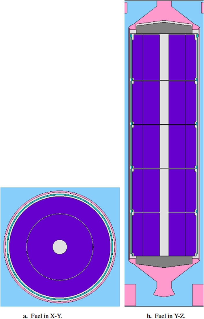
Figure 2. ACRR Fuel. (a) Cross section of fuel in X-Y showing two annular fuel disks. (b) Cross section of fuel in Y-Z showing five niobium cups, upper and lower BeO reflectors, end flutes, and the bottom and top base plates. (Figure not to scale).

Figure 3

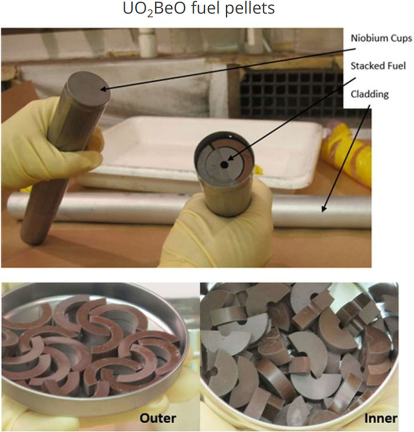
Figure 3. Photograph of fuel and niobium cups showing inner and outer fuel disks (Ames et al., 2022).

Table 1

Table 1. Material and geometric descriptions of the ACRR model core lattice elements. The 90% density fuel elements are identical except for the reduction of the density to 3.09290 ${\mathrm{g}/\mathrm{c}\mathrm{m}}^3$.

In the original model, all 100% density fuel is considered a single material and all 90% fuel is considered a single second material, both of which are enriched to 35 weight ²³⁵U. By using a hexagonal mesh identical to the core lattice, feedback is performed in each lattice position and considers all fuel in that position to be at the same temperature (e.g., no radial variation). In order to investigate the impact of any radial variation in fuel temperature (Section 3.2), the inner fuel disks are assigned one material and the outer a second material for a total of four types of fuel (100% density inner disk, 100% density outer disk, 90% density inner disk, and 90% density outer disk).

2.1.3 Control rod models

There are three types of control rods in the ACRR: fuel-followed control rods, fuel-followed safety rods, and void-followed transient rods. All safety rods move as a single bank, as do all control rods. The transient rods can be fired individually, as a pair followed by a single rod, or individually. Table 1 includes the radial sections of all three types, which have poison sections 52.2478 cm in length for the safety and control rods, and 76.2000 cm in length for the transient rod. The safety and control rods are followed by a stack of five niobium cups, similar to a regular fuel element. The transient rod is followed by an 0.8001 cm radius helium-filled void with an 0.2524 cm thick aluminum 6061-T6 tube assembly.

2.2 Python coupling

Minor modifications to the Python coupling script used in our previous work (Colvin and Palmer, 2025) were made to allow the larger pulse sizes and the refinements used in this work. A hexagonal mesh with the same pitch as the core lattice is used, with each lattice position divided into ten axial nodes. The fission energy generated within each node is calculated by a Serpent detector applying an ENDF reaction type −8 response function (“macroscopic total fission energy production cross section”), $\kappa {\mathrm{\Sigma }}_f$, where $\kappa$ is the average energy released per fission, including prompt and delayed gammas, and ${\mathrm{\Sigma }}_f$ is the macroscopic fission cross section. This is applied to the flux in the fuel as shown in Equation 1,

$E_i^n={\int }_{t_{i-1}}^{t_i}{\int }_{{\mathbf{r}}_{n-1/2}}^{{\mathbf{r}}_{n+1/2}}\kappa {\mathrm{\Sigma }}_f\left(\mathbf{r}\right)\varphi \left(\mathbf{r},t\right)d\mathbf{r}dt,(1)$

to provide the energy produced in the $n$th fuel node in the $i$th time step, where $\varphi$ is the flux, $t$ is time, and $\mathbf{r}$ is position.

As with other pulsed operation analyses (Marcum et al., 2012), this simulation assumes adiabatic conditions due to the extremely short time scale involved. Thus, the temperature in each node at the end of a time step is calculated by

$T_i=T_{i-1}+\frac{\mathrm{\Delta }{E}_i}{m{c}_{\text{eff}}\left(T_{i-1}\right)},(2)$

where $i$ the time step index, $T$ is the temperature of the node at the end of the time step, $\mathrm{\Delta }E$ represents the fission energy generated in the node, and $m$ is the mass of the node. In order to avoid exceeding the limits of the BeO thermal scattering cross section libraries, an additional conditional statement passes “1200.0” to Serpent for any temperature above 1200 K. A Python function was created for the specific heat capacity, allowing easy switching between values and functions of specific heat capacity by defining a variable at the beginning of the Python coupling file. The impact of fuel density on specific heat capacity is assumed to be negligible; the 90% density fuel uses the same function for $C_p(T)$ in Equation 2 as the 100% density fuel. The difference between the two fuel densities in Equation 2 occurs in the calculation of nodal fuel mass. These fuel elements contribute little to the overall reactor power, as they are exclusively located on the periphery of the core.

2.2.1 Multiphysics coupling iteration and convergence

Previous simulations had defaulted to performing two iterations for each time step without checking for convergence of either power or temperature fields. To determine if convergence was, in fact, being reached or if additional iterations would improve the results, a convergence test was added into the Python script. Wu and Kozlowski (2015) used an approach that was slightly modified into a convergence test for this model. Rather than use a set of axial nodes, the ACRR model uses the set of nodes already in place for the multiphysics feedback. After the second iteration, the relative difference in nodal energy generation between the two iterations is compared to $\epsilon$, the relative statistical error in $k_{\mathit{eff}}$ as shown in Equation 3:

$\frac{|E^{\left(2\right)}-E^{\left(1\right)}|}{E^{\left(1\right)}}<\epsilon ,(3)$

where $E$ is the energy generated in a given node over a time step. In the case that $E^{(1)}=0$, $E^{(2)}$ is used as the denominator. This primarily occurs in very low power nodes at the ends of the fuel elements. Because Serpent uses delta-tracking for neutron transport, detectors use the collision estimate of neutron flux, small, low power volumes see poor detector efficiency (Leppänen, 2015). If better data is desired for these nodes, the number of particle histories per time step can be increased. This convergence criterion is used only for this single, first check.

Subsequent iterations test for convergence using the relative statistical error in energy generation for each node as calculated by Serpent. The statistical error is calculated and convergence is checked using the criterion

$E_1^n-2{\sigma }_1^n\le E_2^n\le E_1^n+2{\sigma }_1^n.(4)$

For a time step to be considered converged, 95% of the nodes must fulfill this criterion ($6250\times 95\%=5937.5$, requiring 5938 nodes to meet the conditions of Equation 4).

2.3 Development of alternate specific heat capacity values

Pelfrey (2019) calculated an effective specific heat capacity² of the ACRR fuel using the rule of mixtures as shown in Equation 5:

$c_{\text{eff}}=V_m{c}_m+V_u{c}_u\left(\frac{J}{kg-K}\right),(5)$

where $V_m$ and $c_m$ are the volume fraction and specific heat capacity of the matrix (BeO) and $V_u$ and $c_u$ are the same for the particulate (${\text{UO}}_2$). This work found the effective specific heat capacity to be Equation 6,

$\begin{array}{l}\hfill c_{\text{eff}}=1.11\times 10^{-15}{T}^6+8.84\times 10^{-12}{T}^5-2.75\times 10^{-8}{T}^4\\ \hfill +4.31\times 10^{-5}{T}^3-0.036T^2+16.78T-1706\left(\frac{J}{kg-K}\right),\end{array}(6)$

where $T$ is the temperature in Kelvin. In Colvin and Palmer (2025), this was used along with a constant specific heat capacity derived from a heat capacity determined by the ACRR operations team and the total mass of fuel in the ACRR as shown in Equation 7:

$c_{\text{eff}}=\frac{C}{M}=\frac{0.325\times 10^{6}J/K}{352.6008kg}=921.7222\left(\frac{J}{kg-K}\right).(7)$

Although there is insufficient information to replicate the derivation of Equation 6, this function for specific heat capacity was considered based on interest from Sandia National Laboratories, the sponsoring organization.

A new function for specific heat capacity was developed beginning from the same rule of mixtures (Equation 5) as Pelfrey (2019): Returning to the sources used by Pelfrey (2019), the specific heat capacity of BeO (International Atomic Energy Agency, 2008) from $298\le T\le 1200$ K is shown in Equation 8:

$c_p=1.455+0.606\times 10^{-3}T-0.544\times 10^5{T}^{-2}\left(\frac{kJ}{kg-K}\right)(8)$

and then from $1200\le T\le 2820$ K, the specific heat capacity is shown in Equation 9:

$c_p=1.791+0.201\times 10^{-3}T\left(\frac{kJ}{kg-K}\right).(9)$

The specific heat capacity of ${\text{UO}}_2$ (Fink, 2000) from $298.15\le T\le 3120$ K is shown in Equation 10:

$\begin{array}{ll}\hfill c_p& =0.1940+3.270\times 10^{-4}T-3.132\times 10^{-7}{T}^2+1.173\times 10^{-10}{T}^3\hfill \\ \hfill & -9.791\times 10^{-15}{T}^4-2.654\times 10^3{T}^{-2}\left(\frac{J}{kg-K}\right).\hfill \end{array}(10)$

Using a particulate volume fraction $V_u=0.069$ and matrix volume fraction $V_m=0.931$ (Pelfrey, 2019), the ${\text{UO}}_2$-BeO fuel has an effective specific heat capacity given by Equation 11:

$\begin{array}{ll}\hfill c_{\text{eff}}& =1.35\times 10^3+5.64\times 10^{-1}T-2.16\times 10^{-8}{T}^2+8.09\times 10^{-12}{T}^3\hfill \\ \hfill & -6.76\times 10^{-16}{T}^4-5.06\times 10^7{T}^{-2}\left(\frac{J}{kg-K}\right)\hfill \end{array}(11)$

from $298.15\le T\le 1200$ K and Equation 12,

$\begin{array}{ll}\hfill c_{\text{eff}}& =1.60\times 10^3+2.26\times 10^{-5}T-2.16\times 10^{-8}{T}^2+8.09\times 10^{-12}{T}^3\hfill \\ \hfill & -6.76\times 10^{-16}{T}^4-1.83\times 10^2{T}^{-2}+1.87\times 10^{-1}{T}^{-3}\left(\frac{J}{kg-K}\right).\hfill \end{array}(12)$

from $1200\le T\le 2820$ K. Considering the coefficients of each term in Equations 11, 12 and the temperature range in the order of $10^2$ to $10^3$ expected in these pulses, these can be further simplified by dropping terms that ultimately contribute a quantity more than four orders of magnitude less than the first term of $1.35\times 10^3$, resulting in Equation 13,

$c_{\text{eff}}=1.35\times 10^3+5.64\times 10^{-1}T-5.06\times 10^7{T}^{-2}\left(\frac{J}{kg-K}\right)(13)$

from $298.15\le T\le 1200$ K and Equation 14,

$c_{\text{eff}}=1.60\times 10^3\left(\frac{J}{kg-K}\right)(14)$

from $1200\le T\le 2820$ K.

The pulse simulations in this work are compared to a set of four pulses performed in early 2023 (see Table 2). Power traces, total energy released during the pulse, and maximum fuel temperature were made available by the operations team for the ACRR. The reactor power used in this work was the average of four individual power channels and it was integrated over the length of the pulse for the total energy released. Maximum fuel temperature was taken from the instrumented fuel elements. Unlike power, there is no measurement of fuel temperature over time as the thermocouples cannot react within the relevant time during a pulse. Given the constraints of this available information, the consideration of alternate specific heat capacity functions presented here is intended to provide a rough investigation of the potential for improvement with different functions. In the future, closely working with the operations team for additional pulse data and/or performing a targeted set of pulses to establish a larger number of data points can provide the necessary data to perform a more sophisticated analysis of the specific heat capacity of BeO-${\text{UO}}_2$ fuel.

Table 2

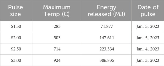
Table 2. Experimental pulse data used for calculation of fuel specific heat capacity.

These sets of energy released and maximum fuel temperature were used to create systems of linear equations which could be solved for expressions for specific heat capacity. Considering Equations 8–10 for temperatures of order $10^2$ to $10^3$, the terms within three orders of magnitude of the maximum are $T^0$, $T^1$, $T^2$, $T^3$, and $T^{-2}$. Having only four datasets, two expressions were considered: a third order polynomial and a rational expression of the form $C(T)=a_0+a_{1}T+a_2{T}^2+a_3{T}^{-2}$.

This evaluation began from the energy balance in Equation 15:

$C\left(T\right)\frac{\partial T}{\partial t}=P\left(t\right),(15)$

where $C(T)$ is the heat capacity of the fuel as a function of temperature $T$ and $P(t)$ is total reactor power as a function of time $t$. While $P(t)$ is directly recorded during a pulse, the only recorded temperature is the maximum fuel temperature as measured by the instrumented fuel elements. An integration over the pulse, shown in Equation 16, eliminated the time dependence:

${\int }_{t=0}^{t=t_f}C\left(T\right)\frac{\partial T}{\partial t}dt={\int }_{t=0}^{t=t_f}P\left(t\right)dt.(16)$

Assuming $C(T)$ to take the form of Equation 17,

$C\left(T\right)={\displaystyle \sum _{n=0}^N}{a}_n{T}^n,(17)$

Equation 16 becomes Equation 18,

${\int }_{t=0}^{t=t_f}{\displaystyle \sum _{n=0}^N}{a}_n{T}^n\frac{\partial T}{\partial t}dt=E_{\mathit{tot}}={\int }_{t=0}^{t=t_f}P\left(t\right)dt.(18)$

Further simplifying Equation 18 for the case of the polynomial expression is shown in Equation 19,

${\int }_{t=0}^{t=t_f}{\displaystyle \sum _{n=0}^N}{a}_n{T}^n\frac{\partial T}{\partial t}dt={\int }_{t=0}^{t=t_f}\frac{\partial }{\partial t}\left[{\displaystyle \sum _{n=0}^N}{a}_n\frac{T^{n+1}}{n+1}\right]dt={\displaystyle \sum _{n=0}^N}\frac{a_n{T}_f^{n+1}}{n+1}-{\displaystyle \sum _{n=0}^N}\frac{a_n{T}_0^{n+1}}{n+1}.(19)$

Finally evaluating this at the bounding times results in Equation 20,

${\displaystyle \sum _{n=0}^N}{a}_n\left[\frac{T_f^{n+1}-T_0^{n+1}}{n+1}\right]=E_{\mathit{tot}}(20)$

With results from four pulses, a third-order polynomial expression for $C(T)$ can be calculated using the system of equations in Equation 21:

$\left[\begin{array}{cccc}\hfill \frac{T_{f,1}-T_i}{1}\hfill & \hfill \frac{T_{f,1}^2-T_i^2}{2}\hfill & \hfill \frac{T_{f,1}^3-T_i^3}{3}\hfill & \hfill \frac{T_{f,1}^4-T_i^4}{4}\hfill \\ \hfill \frac{T_{f,2}-T_i}{1}\hfill & \hfill \frac{T_{f,2}^2-T_i^2}{2}\hfill & \hfill \frac{T_{f,2}^3-T_i^3}{3}\hfill & \hfill \frac{T_{f,2}^4-T_i^4}{4}\hfill \\ \hfill \frac{T_{f,3}-T_i}{1}\hfill & \hfill \frac{T_{f,3}^2-T_i^2}{2}\hfill & \hfill \frac{T_{f,3}^3-T_i^3}{3}\hfill & \hfill \frac{T_{f,3}^4-T_i^4}{4}\hfill \\ \hfill \frac{T_{f,4}-T_i}{1}\hfill & \hfill \frac{T_{f,4}^2-T_i^2}{2}\hfill & \hfill \frac{T_{f,4}^3-T_i^3}{3}\hfill & \hfill \frac{T_{f,4}^4-T_i^4}{4}\hfill \end{array}\right]\left[\begin{array}{c}\hfill a_0\hfill \\ \hfill a_1\hfill \\ \hfill a_2\hfill \\ \hfill a_3\hfill \end{array}\right]=\left[\begin{array}{c}\hfill E_1\hfill \\ \hfill E_2\hfill \\ \hfill E_3\hfill \\ \hfill E_4\hfill \end{array}\right].(21)$

Assuming a starting temperature of 298.15 K and using the experimental data provided in Table 2 then solving and dividing by the total mass of fuel results in the polynomial expression of Equation 22,

$c_{\text{eff}}\left(T\right)=3.04\times 10^{-6}{T}^3-7.24\times 10^{-3}{T}^2+5.87T-614\frac{J}{kg-K}.(22)$

For the rational case, Equation 19 cannot be further generalized and must be evaluated for each $n$ independently. For $0\le n<3$, this does not change from the polynomial case. For $n=3$, the final term is determined with Equation 23:

${\int }_{t=0}^{t=t_f}{a}_3{T}^{-2}\frac{\partial T}{\partial t}dt=a_n\left[-\frac{1}{T_f}+\frac{1}{T_i}\right],(23)$

which then replaces the $a_3$ terms in the coefficient matrix of Equation 21. This results in a final expression for specific heat capacity as shown in Equation 24:

$c_{\mathit{eff}}\left(T\right)=1.45\times 10^{-3}{T}^2-2.59T+2.32\times 10^3-1.15\times 10^8{T}^{-2}.(24)$

All of the values and functions for the specific heat capacity of ${\text{UO}}_2$-BeO fuel are plotted in Figure 4, along with the specific heat capacities of ${\text{UO}}_2$ and BeO individually.

Figure 4

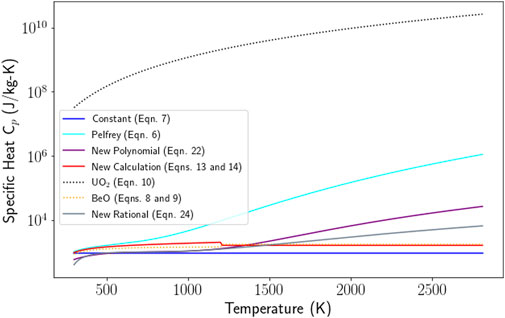
Figure 4. Plot of ${\text{UO}}_2$-BeO fuel specific heat capacities used for modeling and the specific heat capacities of the individual materials ${\text{UO}}_2$ and BeO.

3 Results and discussion

3.1 Single radial region fuel model

Full experimental results for four pulse sizes were available, all performed in 2023. Serpent simulations of the $1.50 and $2.00 pulses were presented previously (Colvin and Palmer, 2025); Table 3 shows the results of all four pulse sizes compared to the experimental results. Figures 5, 8 graphically show the results of a $3.00 pulse, which are broadly representative of all pulse sizes. Comparing the Serpent simulation to the experimental results using the percent absolute relative difference in Equation 25,

$\text{\%\hspace{0.17em}Abs\hspace{0.17em}Rel\hspace{0.17em}Diff}=\frac{|P_{\mathit{exp}}-P_{\mathit{data}}|\left(100\right)}{P_{\mathit{exp}}},(25)$

the “1 Region” columns in Table 3 and the “original fuel” cases in Figure 6 show a closer fit for the constant value for specific heat capacity from Equation 7 over the results from Pelfrey (2019) from Equation 6. All cases have a large difference at the beginning of the pulse, where low power results in noisy experimental data and the instant reactivity insertion assumption results in a small deviation from what would be expected with a realistic rod withdrawal time. To minimize the impact of this early extreme behavior, the first 0.02 s of the simulation (0.01 s of steady state operation and the first 0.01 s of the pulse) have been omitted from the statistics and the median percent absolute relative difference is provided in Table 3 in addition to the mean values.

Table 3

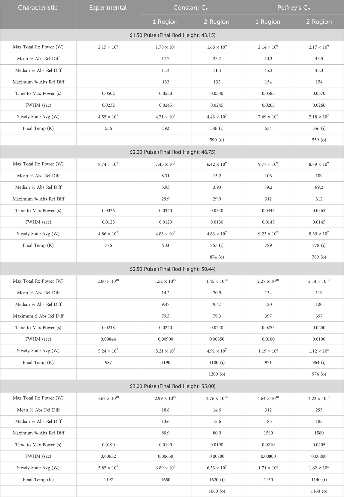
Table 3. Serpent result characteristics for a range of pulse sizes ($1.50, $2.00, $2.50, and $3.00) compared to experimental results. Includes simulations using the constant value for specific heat capacity and Pelfrey’s function for specific heat capacity as a function of temperature, and one and two radial fuel regions. All simulations used a 5 × 10⁻⁴ sec time step. Percent absolute relative difference between experimental and simulated total reactor power considered from the time interval between 0.02 and 0.11 s to reduce the impact of noise in the experimental data.

Figure 5

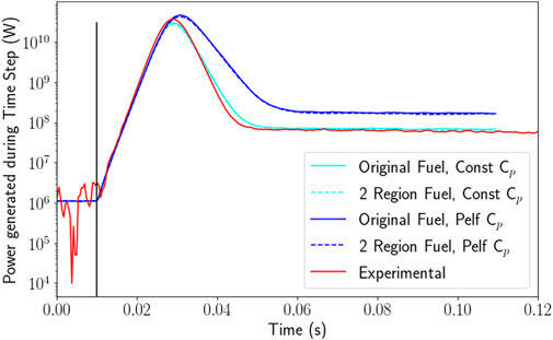
Figure 5. Pulse power as calculated by Serpent compared to experimental results for a $3.00 pulse. Includes simulations using the constant value for specific heat capacity and Pelfrey’s function (Pelfrey, 2019) for specific heat capacity as a function of temperature. Vertical solid black line denotes instantaneous rod withdrawal time. Simulations used one (“original”) or two radial fuel regions and a 5 × 10⁻⁴ s time step.

Figure 6

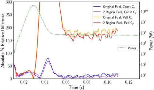
Figure 6. Absolute percent relative difference between experimental data and Serpent simulation results for a $3.00 pulse using both one and two fuel regions and both the constant value for specific heat capacity and Pelfrey’s function (Pelfrey, 2019) for specific heat capacity as a function of temperature. Y-axis scale has been limited to allow constant specific heat capacity results to be meaningfully visible. Peaks for the Pelfrey specific heat capacity results are listed in Table 3.

The power decrease following the peak and the eventual steady state power show the most significant differences between the two specific heat capacity models. During the time increment where power is falling after the peak and the stable power after the pulse, the constant value of specific heat capacity (Equation 7) results in a much closer match to experimental reactor power, at most 30% relative difference ($1.50) and at least 0.57% ($2.50). The simulation using Pelfrey’s function for specific heat capacity (Equation 6) has a more gradual power decrease and stabilizes at a power level significantly above the experimental results, with the closest match ($2.00) having a 90% relative difference and the worst match at a 190% relative difference ($3.00). However, the maximum fuel temperatures reached by each simulation show the opposite relation to the experimental values (as measured by the instrumented fuel elements), with the values from the simulation using Pelfrey’s function for specific heat capacity being much closer to the experimental results. The best match using the constant value for specific heat capacity (Eqn. was the $1.50 pulse, with a relative difference of 5.9%, and the worst was the $3.00 pulse, with a relative difference of 38%. Using Pelfrey’s function for specific heat capacity, the closest match to the experimental fuel temperature is a relative difference of 1.6% ($2.50), while the worst was only 3.5% ($3.00). The higher fuel temperature of the simulation using the constant value for specific heat capacity (Equation 7) explains the steeper drop in temperature after the pulse, as the beryllium oxide in the fuel provides larger amounts of feedback. Although a simulated fuel temperature somewhat above the experimental maximum would be reasonable given that the instrumented fuel elements are limited to a single core position and may not be reading the highest temperature, the constant specific heat capacity simulations showed a temperature significantly above expectations.

The simulations using the constant value for specific heat capacity see small increases in the absolute percent relative difference of total reactor power close to the peak of the pulse but generally even out to be very small as the steady state power is approached after the pulse. The cases using Pelfrey’s function for specific heat capacity, however, show different behavior. All show behavior similar to the constant specific heat capacity at the beginning of the pulse, after which the power begins to diverge. As the power decreases, the absolute percent relative difference increases as the simulation power drops more slowly than the experimental before reaching the steady state power after the pulse. The constant specific heat capacity results in a maximum of 140% absolute relative difference ($1.50), but the median values are all less than 15%. The simulation with Pelfrey’s function for specific heat capacity results in a maximum relative difference of 1580% ($3.00) with the medians falling between 45.0% and 184%.

3.2 Two radial regions fuel model

In an effort to improve the accuracy of the Serpent model, the fuel was divided into two different fuel materials: one for the inner disk and one for the outer, as seen in Figure 2. This allows feedback to occur in 20 nodes per fuel rod: 10 axial nodes in the inner fuel disk region and 10 in the outer. Figure 5 provides a visual representation of the power calculated by simulation with a single radial region (“Original fuel”) and with two radial regions (”2 Region Fuel”) for a $3.00 pulse. The results and statistics of the full range of pulse sizes is also provided in Table 3. Very little change is seen in the statistics of the percent absolute relative difference between simulated total reactor power and experimental data due to the division of the fuel disks into separate feedback nodes. Table 3 displays the absolute percent relative difference between the various simulation results and experimental values as calculated by Equation 25, with six graphically displaying the results for a $3.00 pulse. The only measure that significantly changes is the mean of the relative difference; the median and maximum for one or two region fuel remains the same. In the case of the constant specific heat capacity, the single region fuel is better in all cases except the $3.00. Using Pelfrey’s function for specific heat capacity as a function of temperature, the two region model is better in all cases except the $2.00 pulse. In every case, the difference between the mean values is relatively small: less than 10% for the constant specific heat capacity cases and less than 20% in the Pelfrey cases. To better compare the difference between the one and two region fuel cases for a $3.00 pulse, the difference between the absolute percent relative difference of the two and one region fuel is plotted in Figure 7. While the Pelfrey specific heat capacity simulations generally showed improvement with the two region fuel, especially in the steady state period after the pulse, the constant specific heat capacity results showed very little promise except in the $3.00 case, with the $2.00 and $2.50 simulations only showing a few peaks where the two region fuel model improved the results.

Figure 7

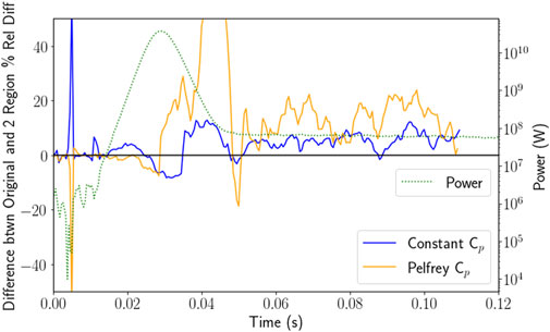
Figure 7. Difference between two and one radial fuel region absolute percent relative differences between experimental data and Serpent simulation results for a $3.00 pulse, using both the constant value for specific heat capacity (Equation 7) and Pelfrey’s function for specific heat capacity as a function of temperature (Equation 6). Positive values indicate the two region fuel model is a closer match to experimental data.

Table 3 includes the maximum fuel temperature which displays a more significant change as well as provides additional information on where the maxima are occurring. Figure 8 provides a graphical representation of the $3.00 pulse fuel temperature results. Using Pelfrey’s function for specific heat capacity, there is less temperature difference between the inner and outer fuel disks than with the constant specific heat capacity. With two fuel regions, both the inner and outer disk temperature were lower than in the single fuel region case. For the two pulse sizes where the experimental maximum temperature was already above the simulated temperature, the change resulting from the additional fuel region is minimal, whereas in the cases where the experimental temperature is below the simulated temperature, the drop is more significant. In the cases with constant specific heat capacity, the impact of the two fuel region model is less consistent. In all cases, the outer fuel disk is at a higher temperature than the inner fuel disk and in some cases may be higher than the single region. The $2.00 pulse is an outlier as the only pulse size where there is a significant shift of both the inner and outer fuel temperature.

Figure 8

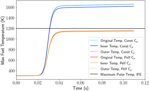
Figure 8. Maximum local fuel temperature as calculated by the Serpent coupling script compared to the maximum experimental pulse temperature for a $3.00 pulse. Includes simulations using the constant value for specific heat capacity and Pelfrey’s function (Pelfrey, 2019) for specific heat capacity as a function of temperature. Vertical solid black line denotes instantaneous rod withdrawal time. Simulations used one (“original”) or two radial fuel regions and a 5 × 10⁻⁴ s time step.

3.3 Increased iterations for convergence

Except for the initial time step, all time steps converged on the third iteration (the first to use the convergence criterion based on the relative error). As shown in Figure 9 and confirmed in Figure 10, there is very little difference in the total reactor power between the original simulation and the one with the added convergence criterion. The primary difference lay in the maximum fuel temperature, with the converged case reaching a slightly lower maximum fuel temperature. Both of these cases used the constant specific heat capacity and $10^6$ histories divided into 20 batches for each iteration (because the neutron and neutron precursor distributions at the end of one time step are saved for use at the beginning of the next, these are external source simulations rather than criticality simulations).

Figure 9

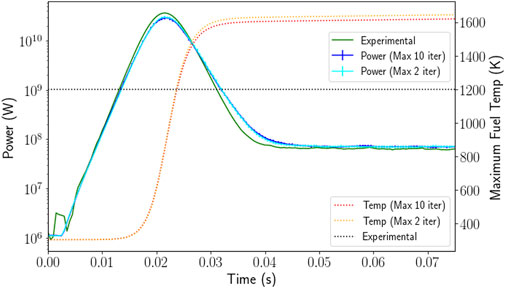
Figure 9. Plots of power and temperature for a $3.00 pulse simulation using the original two iterations per time step compared to a simulation checking for convergence and allowing up to ten iterations. Simulation performed using the constant value for specific heat capacity (Equation 7).

Figure 10

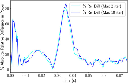
Figure 10. Plot of the percent absolute relative difference between Serpent results and experimental results for a $3.00 pulse. Serpent results are shown for the original two iterations per time step and the case checking for convergence and allowing up to ten iterations. Simulation performed using the constant value for specific heat capacity (Equation 7).

3.4 Alternate functions for fuel specific heat capacity

The range of specific heat capacity functions shown in Figure 4 were used in a series of $3.00 pulse simulations, with the results presented in Figure 11 and Table 4. The original constant value for specific heat capacity remains the closest match for the full width-half maximum. The rational function provides a slight improvement to the final steady state average power over the original constant value for specific heat capacity, with a 16% percent absolute relative difference over 19%. The best match for the maximum power is actually the new function calculated from the individual properties of ${\text{UO}}_2$ and BeO (Equation 13 and 14), though the new third order polynomial calculated from experimental data (Equation 22) results in only slightly worse results, with percent absolute relative differences of 11% and 12%, respectively. The original function from Pelfrey (Equation 6) remains the closest final temperature to the maximum temperature of the pulse, though it is also the only specific heat capacity model to underpredict the maximum temperature (by 42 K). The third order polynomial result (Equation 22) is the closest match of the remaining models, overpredicting the maximum temperature by 131 K.

Figure 11

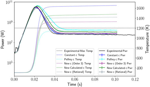
Figure 11. Plot of $3.00 pulse simulations performed using different specific heat capacities.

Table 4

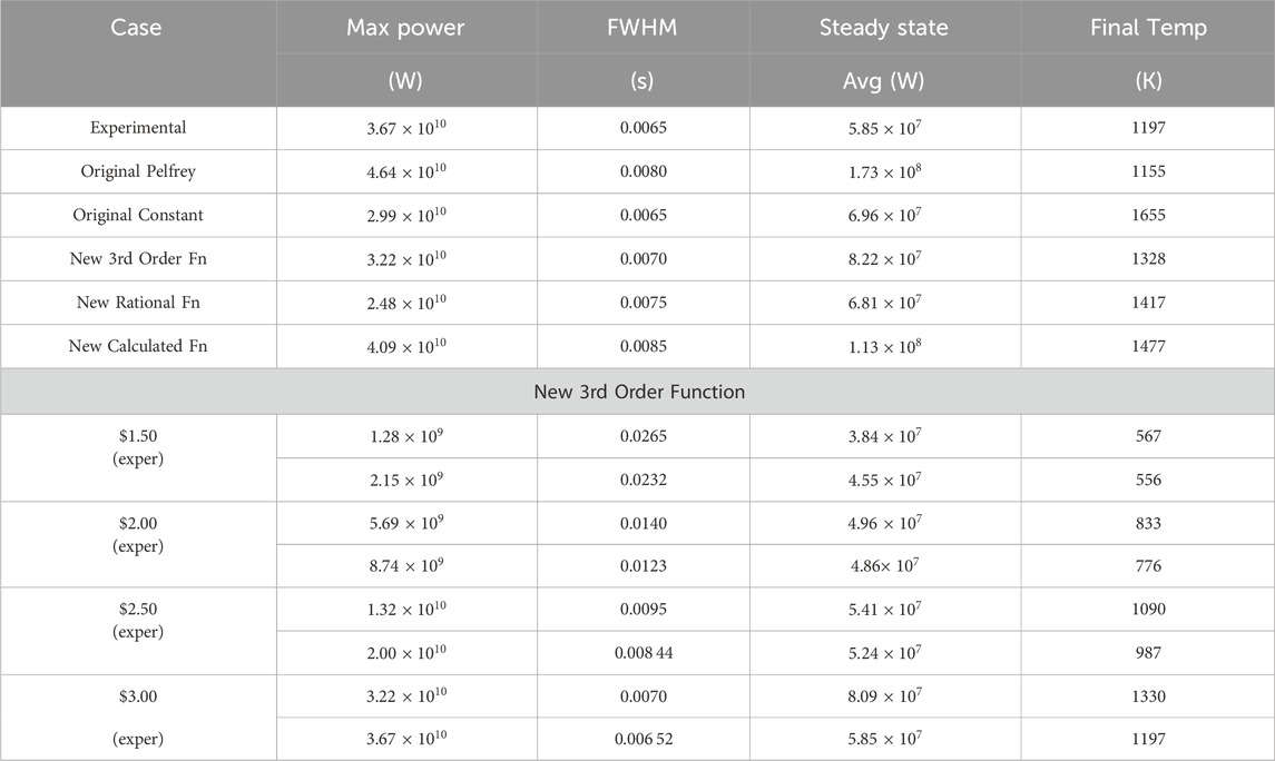
Table 4. Characteristics of $3.00 pulse using several functions for specific heat capacity compared to experimental results. Further exploration of the new third order function for all pulse sizes.

To further assess the third order polynomial, simulations were performed for the other three pulse sizes. The third order polynomial was chosen over the rational function for its better match in maximum power, pulse width, and final temperature, although the rational function more closely matched the steady state average power after the pulse. Results are shown in Table 4. A $1.50 pulse simulation using the third order polynomial function significantly underpredicts the power, though less pronounced than in larger pulses. Use of the third order polynomial function for specific heat capacity in simulations of all four pulse sizes results in the underprediction of maximum pulse power, though only in the case of the $1.50 pulse is the steady state final power also underpredicted. Additionally, using the third order polynomial specific heat capacity produces a narrower pulse, as measured by the full width-half maximum value in all pulse sizes. Finally, in all pulse sizes, the maximum fuel temperature remains above the maximum temperature measured experimentally, with smaller differences between predicted and measured temperature at smaller pulse sizes. This is in keeping with the expectation of a “true” maximum fuel temperature above the experimentally measured value.

4 Conclusion

Simulations using our model have now been compared to experimental results for four pulse sizes across the range of pulse sizes performed at the ACRR. As with the $1.50 and $2.00 pulse results presented previously (Colvin and Palmer, 2025), the constant value for specific heat capacity (Equation 7) is a closer match to the experimental power results than Pelfrey’s specific heat capacity as a function of temperature (Equation 6). However, Pelfrey’s function outperforms in terms of expected maximum fuel temperature. The division of the fuel into two radial regions did not yield consistent improvement except in the post-pulse steady state power in the simulations using Pelfrey’s function. Nor did the introduction of a convergence criterion improve the power results significantly, with only a slight improvement to the prediction of the maximum fuel temperature. The most significant modifications to the model are achieved through the specific heat capacity, with the third order polynomial (Equation 22) improving the maximum fuel temperature prediction over that of the constant value by over 200 K with a relatively small loss in the power prediction.

There is still the potential for improvement in modeling pulses in the ACRR. The addition of a temperature field convergence check may further improve the results, though an acceptable criterion would need to be developed. Additionally, an increase in the number of particle histories in each iteration would decrease the statistical error and tighten the convergence criterion for each node. The drawback of this would be that both the increased histories per iteration and potential increased number of iterations per time step would lengthen the overall time for the simulation. With the larger pulse sizes, there remains the need for actual thermal scattering cross section data for BeO above 1200 K. The specific heat capacity of the fuel remains an open question. A larger survey of pulse data may yield a better fit for the specific heat capacity as a function of temperature, or a second materials science analysis combined with pulse results may shed light on the best model for the specific heat capacity. It may also prove useful to transition to a piecewise continuous model for specific heat capacity, as BeO is known to be in this temperature range. The difference in the heat capacity of the 100% fuel density elements and the 90% fuel density elements is also a potential area for model refinement, particularly if more detailed information on the fuel condition in these elements is desired. Finally, there may also be additional improvement using some of these less hopeful techniques in conjunction, e.g., the use of a convergence criterion with the two radial region fuel.

Data availability statement

The datasets presented in this article are not readily available because we do not have permission to release our data. Requests to access the datasets should be directed to Y29sdmluZW1Ab3JlZ29uc3RhdGUuZWR1.

Author contributions

EC: Conceptualization, Methodology, Software, Visualization, Writing – original draft, Writing – review and editing. TP: Conceptualization, Funding acquisition, Project administration, Resources, Supervision, Writing – original draft, Writing – review and editing.

Funding

The author(s) declare that financial support was received for the research and/or publication of this article. This research was funded through a partnership with Sandia National Laboratories. Sandia National Laboratories is a multimission laboratory managed and operated by National Technology and Engineering Solutions of Sandia, LLC, a wholly owned subsidiary of Honeywell International Inc., for the U.S. Department of Energy’s National Nuclear Security Administration under contract DE-NA0003525. This paper describes objective technical results and analysis. Any subjective views or opinions that might be expressed in the paper do not necessarily represent the views of the U.S. Department of Energy or the United States Government.

Acknowledgments

The authors would like to thank Jaakko Leppänen, Ville Valtavirta, and the Serpent team at VTT Technical Research Centre of Finland for their help in troubleshooting. We would also like to thank Keenan Hoffman and Christopher Magone for their help in the MCNP-to-Serpent model conversion.

Conflict of interest

The authors declare that the research was conducted in the absence of any commercial or financial relationships that could be construed as a potential conflict of interest.

The handling editor MD shares an affiliation of the authors EC and TP. All parties confirm the absence of any collaboration during review.

Generative AI statement

The author(s) declare that no Generative AI was used in the creation of this manuscript.

Publisher’s note

All claims expressed in this article are solely those of the authors and do not necessarily represent those of their affiliated organizations, or those of the publisher, the editors and the reviewers. Any product that may be evaluated in this article, or claim that may be made by its manufacturer, is not guaranteed or endorsed by the publisher.

Footnotes

¹Fuel Element Assembly Drawing P59525.

²The authors have used “heat capacity” $(C)$ and “specific heat capacity” $(c)$ in this work for clarity, regardless of the language used in the sources.

References

Ames, D., Cole, J., Cook, M., Raster, A., Harms, G., and Miller, J. (2022). “IER-523: feasibility of experiments focused on measuring the effects of UO₂BeO material on critical configurations using 7uPCX,” in 2022 DOE nuclear criticality safety program technical program review. SAND2022-1412 PE.

Google Scholar

Colvin, E., and Palmer, T. S. (2025). High-fidelity multiphysics modeling of pulsed reactor heat generation in the Annular Core Research Reactor fuel using Serpent 2. Ann. Nucl. Energy 211, 110954. doi:10.1016/j.anucene.2024.110954

CrossRef Full Text | Google Scholar

DePriest, K. R., Cooper, P. J., and Parma, E. J. (2006). MCNP/MCNPX model of the annular core research reactor. Albuquerque, NM: Sandia National Laboratories.

Google Scholar

Fink, J. K. (2000). Thermophysical properties of uranium dioxide. J. Nucl. Mater. 279, 1–18. doi:10.1016/s0022-3115(99)00273-1

CrossRef Full Text | Google Scholar

International Atomic Energy Agency (2008). Thermophysical properties of materials for nuclear engineering: a tutorial and collection of data. Vienna, Austria: International Atomic Energy Agency.

Google Scholar

Leppänen, J. (2015). Serpent - a continuous-energy Monte Carlo reactor physics burnup calculation code user’s manual. Finland: VTT Technical Research Centre of Finland. Available online at: https://serpent.vtt.fi/serpent/download/Serpent_manual.pdf.

Google Scholar

Marcum, W. R., Palmer, T. S., Woods, B. G., Keller, S. T., Reese, S. R., and Hartman, M. R. (2012). A comparison of pulsing characteristics of the Oregon State University TRIGA reactor with FLIP and LEU fuel. Nucl. Sci. Eng. 171, 150–164. doi:10.13182/nse11-25

CrossRef Full Text | Google Scholar

Parma, E. J., and Gregson, M. W. (2019). The annular core research reactor (ACRR) description and capabilities. Albuquerque, NM: Sandia National Laboratories.

Google Scholar

Parma, E. J., Naranjo, G. E., Lippert, L. L., Clovis, R. D., Martin, L. E., Kaiser, K. I., et al. (2017). Radiation characterization summary: ACRR-FRECII cavity free-field environment at the core centerline (ACRR-FRECII-FF-cl). Albuquerque, NM: Sandia National Laboratories.

Google Scholar

Parma, E. J., Naranjo, G. E., Lippert, L. L., and Vehar, D. W. (2016). Neutron environment characterization of the central cavity in the annular core research reactor. In EPJ Web Conf., vol. 106, 01003, doi:10.1051/epjconf/201610601003

CrossRef Full Text | Google Scholar

Pelfrey, E. (2019). A transient thermal and structural analysis of fuel in the annular core research reactor. Master’s thesis, University of New Mexico.

Google Scholar

Talley, D. G., and Shen, Y.-L. (2020). RAZORBACK–a reactor transient analysis code for large rapid reactivity additions in a natural circulation research reactor. Ann. Nucl. Energy 138, 107153. doi:10.1016/j.anucene.2019.107153

CrossRef Full Text | Google Scholar

Viitanen, T., and Leppännen, J. (2012). Explicit treatment of thermal motion in continuous-energy Monte Carlo tracking routines. Nucl. Sci. Eng. 171, 165–173. doi:10.13182/nse11-36

CrossRef Full Text | Google Scholar

Viitanen, T., and Leppännen, J. (2014). Target motion sampling temperature treatment technique with elevated basis cross-section temperatures. Nucl. Sci. Eng. 177, 77–89. doi:10.13182/nse13-37

CrossRef Full Text | Google Scholar

Williamson, R. L., Hales, J. D., Novascone, S. R., Pastore, G., Gamble, K. A., Spencer, B. W., et al. (2021). BISON: a flexible code for advanced simulation of the performance of multiple nuclear fuel forms. Nucl. Technol. 207, 954–980. doi:10.1080/00295450.2020.1836940

CrossRef Full Text | Google Scholar

Wu, X., and Kozlowski, T. (2015). Coupling of system thermal-hydraulics and Monte-Carlo code: convergence criteria and quantification of correlation between statistical uncertainty and coupled error. Ann. Nucl. Energy 75, 377–387. doi:10.1016/j.anucene.2014.08.016

CrossRef Full Text | Google Scholar