Comparison of spatial dynamics and point kinetics approaches in multiphysics modeling of the molten salt reactor experiment

In this work, we present validation test results of fully coupled neutronics and thermal-hydraulics models of the Molten Salt Reactor Experiment (MSRE) against experimental data of the zero power pump transients and the natural circulation tests at low power. To capture the strong coupling between neutronics and thermal-hydraulics due to fuel circulation, and to account for the delayed neutron precursor (DNP) distribution, the porous media thermal-hydraulics solver Pronghorn was fully coupled to the spatial neutron dynamics code Griffin, which solves the neutron diffusion equation, and to the 0-D point kinetics solver Squirrel, using a 2-D homogenized representation of the MSRE. The validation test results show very good agreement with experimental data for both point kinetics and spatial dynamics simulations, capturing the strong feedback effect and DNP losses in the MSRE. The 0-D code Squirrel accurately predicted the time-dependent behavior in the MSRE given the steady-state spatial dynamics solution of Griffin.

1 Introduction

The Molten Salt Reactor Experiment (MSRE) was conducted in the 1960s at Oak Ridge National Laboratory. It provided important experimental experience and data on the operation of molten-salt reactors (MSRs) with liquid flowing fuel (Haubenreich and Engel, 1970). The MSRE fuel was dissolved in liquid salt, which flowed through the core, simultaneously generating and extracting heat. The flowing salt distinguishes MSRs from other reactor designs. In such reactors, the fluid dynamics and neutronics are strongly coupled through a large negative temperature feedback due to salt expansion and Doppler broadening (Serp et al., 2014).

The strong thermal feedback and the redistribution of the delayed neutron source in the core (Kerlin et al., 1971a) require a different treatment compared to other advanced reactor designs (Locatelli et al., 2013). The flowing fuel distinguishes MSRs from solid fuel reactors, and modeling the behavior of MSRs necessitates a tightly coupled multiphysics simulation that accounts for fuel flow, thermal feedback, and the shifting of the delayed neutron source due to advection of the delayed neutron precursors (DNPs). Even though the delayed neutron fraction is small, the change in the effective reactivity reserve needs to be accounted for.

With the renewed interest in MSRs, more appropriate modeling tools are being developed. Oak Ridge National Laboratory developed one of the pioneering programs to analyze DNP movement in the MSRE in the 1960s (Ball and Kerlin, 1965). Since the inception of that program, several projects have developed new analysis tools dedicated to MSRs (SAMOFAR, 2025; SAMOSAFER, 2025; EVOL, 2025; GeNFOAM, 2025). The Monte Carlo N-Particle (Kophaiza et al., 2004) and Serpent codes (Aufiero et al., 2014) are actively being developed to account for the changed delayed neutron source. To enable transients, deterministic methods are used, such as GeN-Foam (Fiorina et al., 2015), which combines coars mesh thermal hydraulics with a deterministic neutronics code capable of modeling the impact of DNP drift (Shi et al., 2020). Several low-fidelity codes, such as the MOlten SAlt Incompressible Calculation System known as MOSAICS (Mascaron et al., 2023), LiCore (Laureau et al., 2021), and the System Analysis Module (SAM) (Fang et al., 2020), have shown the ability to evaluate transients in MSRs on a system code level.

Idaho National Laboratory is actively working on modeling the MSRE by coupling the thermal-hydraulics codes Pronghorn (Novak et al., 2021) and SAM (Hu et al., 2021) to the neutronics solver Griffin (Wang et al., 2025). These efforts have shown that Pronghorn and Griffin (Schunert et al., 2023; Jaradat et al., 2024) and SAM and Griffin (Jaradat et al., 2023) can be successfully coupled to model MSRs. Also, the Griffin-SAM coupling has been validated against MSRE zero power pump transients (Jaradat and Ortensi, 2023). Griffin solves the neutron diffusion equation with discrete energy groups. The DNP drift is evaluated by reconstructing the delayed flux from the DNP field provided by Pronghorn.

Since 2023 researchers at the Technical University of Denmark have been developing the modified Point Kinetics (PK) solver Squirrel into the MOOSE framework. It is able to account for spatial deviations in the DNP field (Pfahl et al., 2025) by weighting the spatial DNP field with the adjoint flux. Additionally, Squirrel can estimate the temperature feedback by weighting the change in temperature with the adjoint flux. The importance of spatially weighting the DNPs during transients is discussed in (Habtemariam et al., 2024).

In this work, we compare the solutions of the neutron spatial dynamics Griffin and the 0-D neutronics solver Squirrel coupled to Pronghorn for modeling the MSRE under the MOOSE framework. The model and the coupling scheme between Pronghorn and Griffin or Squirrel are validated against the experimental data obtained from the MSRE reports. The validation is done for three different transients: pump start-up, pump coast-down, and natural circulation. Furthermore, the neutronics codes are verified against each other. The verification and validation are done within the same reactor model and on the same mesh. This approach allows for a detailed comparison of the PK solver and the spatial neutron dynamics solver codes with a consistent thermal-hydraulics simulation. Isolating the results of the neutronics codes from the thermal-hydraulics simulation enables a detailed comparison of the differences in the simulation results of both neutronics codes.

This paper is structured as follows: Section 2 provides a description of the solvers used in the analyses and discusses the coupling scheme between the neutronics and thermal-hydraulics codes. Section 3 presents the developed computational model of the MSRE and the modeling assumptions. Section 4 presents the simulation results for a static reactor at 8 MW obtained by Griffin coupled with Pronghorn, including the temperature field, the flow field, and the evaluated temperature coefficients. The static reactivity loss due to the DNP advection is calculated with Griffin and Squirrel for ²³⁵U and ²³³U fuels. Furthermore, the simulation results calculated with both neutronics codes are validated against the experimental data from the pump start-up, pump coast-down, and natural circulation transients. Additionally, the simulated DNP density during the pump start-up and the simulated power density and salt temperature during the natural circulation transient are discussed. Finally, Section 5 provides a summary and the conclusions of the study.

2 Analysis methodology

The methodology used in the neutronics codes Griffin and Squirrel and the coarse-mesh thermal-hydraulics code Pronghorn to obtain the flowing-fuel solutions are introduced in this section. Also, the multiphysics coupling scheme between the neutronics and thermal hydraulics, including the advection of the DNPs, is presented.

2.1 Neutronics methods

In the neutronics calculations we employ the spatial neutron diffusion code (Griffin) and the 0-D PK solver (Squirrel) to model the effect of the flowing fuel and the redistribution of DNPs during steady-state and transient calculations. The solutions of Squirrel, which is a modified PK solver for flowing-fuel MSRs, are verified against the solutions of Griffin’s diffusion solver. Squirrel can account for the time-dependent spatial distribution of the DNPs in the reactor by considering a proper weighting function.

2.1.1 Griffin: spatial dynamics solver

Griffin is a deterministic neutronics solver for analyzing advanced reactors. It can analyze the flowing-fuel behavior in MSRs (Jaradat et al., 2024) by calculating the prompt and delayed fission source separately. The delayed fission source is calculated using the advected DNP field provided by Pronghorn. The delayed fission source is then added to the prompt fission source to obtain the total flux. Griffin solves the linearized Boltzmann equation

$\begin{array}{l}\hfill \frac{1}{v_g}\frac{\partial {\varphi }_g\left(t,\mathbf{r}\right)}{\partial t}=\nabla \cdot D_g\left(t,\mathbf{r}\right)\nabla {\varphi }_g\left(t,\mathbf{r}\right)-{\mathrm{\Sigma }}_{t,g}\left(t,\mathbf{r}\right){\varphi }_g\left(t,\mathbf{r}\right)+{\displaystyle \sum _{g^{\prime }=1}^G}{\mathrm{\Sigma }}_{s,g^{\prime }\to g}\left(t,\mathbf{r}\right){\varphi }_{g^{\prime }}\left(t,\mathbf{r}\right)\\ \hfill +\frac{\left(1-\beta \right){\chi }_{p,g}}{k_{\mathit{eff}}}{\displaystyle \sum _{g^{\prime }=1}^G}\bar{\nu }{\mathrm{\Sigma }}_{f,g^{\prime }}\left(t,\mathbf{r}\right){\varphi }_{g^{\prime }}\left(t,\mathbf{r}\right)+\frac{1}{k_{\mathit{eff}}}{\displaystyle \sum _{i=1}^I}{\chi }_{d,g,i}{\lambda }_i{c}_i\left(t,\mathbf{r}\right),\end{array}(1)$

where ${\varphi }_g(t,\mathbf{r})$ is the neutron flux at time $t$, at position $\mathbf{r}$, and of energy group $g$. ${\mathrm{\Sigma }}_t$, ${\mathrm{\Sigma }}_s$, and ${\mathrm{\Sigma }}_f$ are the total, scattering, and fission macroscopic cross sections, respectively. $k_{\mathit{eff}}$ is the eigenvalue of the system, $\bar{\nu }$ is the neutron yield per fission, $\beta$ is the total delayed neutron fraction, $D$ is the diffusion coefficient, $v$ is the neutron velocity, ${\chi }_p$ and ${\chi }_d$ are the prompt and delayed neutron spectra, $c_i$ and ${\lambda }_i$ are the DNPs of group $i$ and it’s corresponding decay constant. The term ${\sum }_{i=1}^I{\chi }_{d,g,i}{\lambda }_i{c}_i(t,\mathbf{r})$ represents the delayed neutron source, which can be determined by solving the DNP concentration equations for MSRs with flowing fuel. Modeling flowing fuel introduces an extra term to the DNP equations to account for the drift of DNPs in the core, and their decay outside the core as given in Equation 2 for the $i^{\text{th}}$ group:

$\frac{\partial c_i\left(t,\mathbf{r}\right)}{\partial t}={\beta }_i{\displaystyle \sum _{g^{\prime }=1}^G}\bar{\nu }{\mathrm{\Sigma }}_{f,g^{\prime }}\left(t,\mathbf{r}\right){\varphi }_{g^{\prime }}\left(t,\mathbf{r}\right)-{\lambda }_i{c}_i\left(t,\mathbf{r}\right)-\nabla \cdot \mathbf{U}\left(t,\mathbf{r}\right)c_i\left(t,\mathbf{r}\right),i=1,\dots ,I,(2)$

where $\mathbf{U}$ is the fuel salt velocity, and ${\beta }_i$ the delayed neutron fraction of group $i$. The advection term $\nabla \cdot (\mathbf{U}(t,\mathbf{r})c_i(t,\mathbf{r}))$ is added to the DNP equations to account for the DNP movement due to fuel flow, while the diffusion of DNPs is not considered in this work. Equation 2 is solved along with the homogeneous boundary condition to determine the concentrations of the DNPs at the core inlet, taking into account their decay while residing in the outer loop. Equations 1, 2 are strongly coupled through the delayed neutron source and the fission source. By including the advection term in the DNP tracking, the tight multiphysics coupling is expanded with the thermal-fluids code.

In the current work, the fission source is provided to the thermal-fluids code Pronghorn. The resulting distribution of DNPs obtained from the thermal-fluids code, is then transferred to Griffin. With the delayed neutron source Griffin can calculate the total neutron flux.

Griffin does not have the capability to calculate the kinetics parameters for flowing-fuel reactors, which require a more sophisticated approach to obtain the adjoint solution of the system. However, Griffin does calculate the kinetics parameters of stationary fuel reactors, which can be used to obtain the effective delayed neutron fraction for flowing fuel $({\beta }_{\mathit{flow}})$ as

${\tilde{\beta }}_{\mathit{flow}}={\tilde{\beta }}_{\mathit{static}}+{\rho }_{\mathit{flow}},(3)$

where ${\rho }_{\mathit{flow}}$ is the reactivity loss due to the DNPs advection with the fuel flow and the decay of the DNPs. This reactivity change can be calculated by taking the reciprocal difference of the stationary fuel eigenvalue $k_{\mathit{eff}}^{\mathit{static}}$ and the flowing-fuel eigenvalue $k_{\mathit{eff}}^{\mathit{flow}}$:

${\rho }_{\mathit{flow}}={\left(k_{\mathit{eff}}^{\mathit{static}}\right)}^{-1}-{\left(k_{\mathit{eff}}^{\mathit{flow}}\right)}^{-1}.(4)$

In Griffin three feedback mechanisms are considered in modeling MSRs:

• Temperature: affects the fuel salt (Doppler) and solid moderator microscopic cross sections.

• Density: affects concentration of the salt nuclides within the core due to fuel salt expansion.

• Velocity: affects DNP distributions in the core and outer loop.

In Griffin, the thermal feedback coefficient of the fuel salt accounts for changes in microscopic cross section and fuel salt expansion due to temperature and corresponding density changes. The thermal feedback coefficient of the reactor is then calculated by changing the temperature by $\mathrm{\Delta }T$ globally, and as a result the density, relative to the temperature in a reference simulation. The temperature feedback coefficient $(\mathrm{\Gamma })$ is then calculated from the ratio of the reactivity change to the temperature change as

$\mathrm{\Gamma }=\frac{{\left(k_{\mathit{eff}}^{T_1}\right)}^{-1}-{\left(k_{\mathit{eff}}^{T_2}\right)}^{-1}}{T_2-T_1}.(5)$

2.1.2 Squirrel: point kinetics solver

Squirrel is a PK solver developed for the transient analysis of MSRs (Pfahl et al., 2025) under the MOOSE framework. Squirrel solves a modified version of the PK equation to account for the advection of DNPs in the core and their decay outside the core by weighting the time-dependent DNPs with an importance function spatially, and it accounts for temperature distribution changes in the reactor. The details of the derivation of the PK equation for MSR applications is described in Mattioli et al. (2021) and will be discussed briefly in this section.

The PK formulation used in Squirrel is derived from the multigroup neutron flux equations by integrating Equations 1, 2 over energy and assuming a critical reactor so that $k_{\mathit{eff}}=1$ yields the one group flux equation as

$\begin{array}{l}\hfill \frac{1}{v}\frac{\partial \varphi \left(t,\mathbf{r}\right)}{\partial t}=\nabla \cdot D\left(t,\mathbf{r}\right)\nabla \varphi \left(t,\mathbf{r}\right)-{\mathrm{\Sigma }}_a\left(t,\mathbf{r}\right)\varphi \left(t,\mathbf{r}\right)\\ \hfill +\left(1-\beta \right)\bar{\nu }{\mathrm{\Sigma }}_f\left(t,\mathbf{r}\right)\varphi \left(t,\mathbf{r}\right)+{\displaystyle \sum _{i=1}^I}{\lambda }_i{c}_i\left(t,\mathbf{r}\right),\end{array}(6)$

and the corresponding DNP concentration equation as

$\frac{\partial c_i\left(t,\mathbf{r}\right)}{\partial t}={\beta }_i\bar{\nu }{\mathrm{\Sigma }}_f\left(t,\mathbf{r}\right)\varphi \left(t,\mathbf{r}\right)-{\lambda }_i{c}_i\left(t,\mathbf{r}\right)-\nabla \cdot \mathbf{U}\left(t,\mathbf{r}\right)c_i\left(t,\mathbf{r}\right),i=1,\dots ,I.(7)$

First the one group neutron flux $\varphi (\mathbf{r},t)$ is factored into a purely time-dependent amplitude function $N(t)$ and a time- and space-dependent shape function $\psi (\mathbf{r},t)$ as

$\varphi \left(\mathbf{r},t\right)=N\left(t\right)\psi \left(t,\mathbf{r}\right).(8)$

This factorization is a simple separation of the flux and is not an approximation. This separation is, in general, not unique and requires a second equation to ensure its uniqueness. We use a space integral over the shape function to keep the time dependence in the amplitude function. The chosen constraint condition is given by

$⟨{\varphi }_0^{*}\left(\mathbf{r}\right);\frac{1}{v}\psi \left(t,\mathbf{r}\right)⟩=K_0,(9)$

with the steady-state one group adjoint flux function ${\varphi }_0^{*}(\mathbf{r})$ and a constant $K_0$. ${\varphi }_0^{*}(\mathbf{r})$ is used as the importance weighting function of the reactor.

By multiplying Equation 6 with ${\varphi }_0^{*}(\mathbf{r})$, integrating it over space, and dividing the equation by the static importance-weighted neutron source yields

$\mathrm{\Lambda }\left(t\right)\frac{\text{d}N\left(t\right)}{\text{d}t}=\left(\rho \left(t\right)-\tilde{\beta }\left(t\right)\right)N\left(t\right)+{\displaystyle \sum _{i=1}^I}{\lambda }_i\frac{⟨{\varphi }_0^{*}\left(\mathbf{r}\right)c_i\left(t,\mathbf{r}\right)⟩}{\langle {\varphi }_0^{*}\left(\mathbf{r}\right),\bar{\nu }{\mathrm{\Sigma }}_f\left(t,\mathbf{r}\right)\psi \left(r,\mathbf{r}\right)\rangle }.(10)$

with the following parameters:

• The neutron lifetime

$\mathrm{\Lambda }\left(t\right)=\frac{⟨{\varphi }_0^{*}\left(\mathbf{r}\right);v^{-1}\psi \left(t,\mathbf{r}\right)⟩}{F\left(t\right)}=\frac{K_0}{F\left(t\right)}.(11)$

• The delayed neutron fraction

$\tilde{\beta }\left(t\right)=\frac{⟨{\varphi }_0^{*}\left(\mathbf{r}\right);\beta \bar{\nu }{\mathrm{\Sigma }}_f\left(t,\mathbf{r}\right)\psi \left(t,\mathbf{r}\right)⟩}{F\left(t\right)}.(12)$

• The reactivity

$\begin{array}{c}\rho \left(t\right)=\frac{⟨{\varphi }_0^{*}\left(\mathbf{r}\right);\left[\nabla \cdot D\left(t,\mathbf{r}\right)\nabla \psi \left(\mathbf{r},t\right)-{\mathrm{\Sigma }}_a\left(t,\mathbf{r}\right)\psi \left(\mathbf{r},t\right)+\bar{\nu }{\mathrm{\Sigma }}_f\left(t,\mathbf{r}\right)\right]\psi \left(\mathbf{r},t\right)⟩}{F\left(t\right)}.\end{array}(13)$

• The static importance-weighted neutron source

$F\left(t\right)=⟨{\varphi }_0^{*}\left(\mathbf{r}\right),\bar{\nu }{\mathrm{\Sigma }}_f\left(\mathbf{r},t\right)\psi \left(\mathbf{r},t\right)⟩.(14)$

$\mathrm{\Lambda }(t)$ and $\tilde{\beta }(t)$ can be evaluated initially in a steady-state reactor so that the neutron lifetime and the delayed neutron fraction are time independent. The reactivity is split into three parts:

$\rho \left(t\right)={\rho }_{\mathit{temp}}+{\rho }_{\mathit{insertion}}+{\rho }_{\mathit{flow}},(15)$

with ${\rho }_{\mathit{temp}}$ representing the reactivity response due to temperature changes in the reactor, ${\rho }_{\mathit{insertion}}$ the external reactivity insertions, and ${\rho }_{\mathit{flow}}$ the reactivity necessary to keep the reactor critical when fuel is flowing. A common choice in the literature is to substitute the reduced DNP concentration, such as $c_i(\mathbf{r},t)=C_i(\mathbf{r},t)\mathrm{\Lambda }$, into Equation 16. The final PK equations evaluated in Squirrel are

$\left\{\begin{array}{cc}\hfill & \frac{\text{d}N\left(t\right)}{\text{d}t}=\frac{\left({\rho }_{\mathit{temp}}+{\rho }_{\mathit{insertion}}+{\rho }_{\mathit{flow}}-\tilde{\beta }\right)}{\mathrm{\Lambda }}N\left(t\right)+{\displaystyle \sum _{i=1}^I}{\lambda }_i\frac{⟨{\varphi }_0^{*}\left(\mathbf{r}\right)C_i\left(t,\mathbf{r}\right)⟩}{\langle {\varphi }_0^{*}\left(\mathbf{r}\right),\bar{\nu }{\mathrm{\Sigma }}_f\left(\mathbf{r}\right)\psi \left(\mathbf{r}\right)\rangle }.\hfill \\ \hfill & \frac{\partial C_i\left(t,\mathbf{r}\right)}{\partial t}=\frac{{\beta }_i}{\mathrm{\Lambda }}\bar{\nu }{\mathrm{\Sigma }}_f\left(\mathbf{r}\right)N\left(t\right)\psi \left(\mathbf{r}\right)-{\lambda }_i{C}_i\left(t,\mathbf{r}\right)-\nabla \cdot \mathbf{U}\left(t,\mathbf{r}\right)C_i\left(t,\mathbf{r}\right),i=1,\dots ,I.\hfill \end{array}\right.(16)$

Squirrel relies on a thermal-hydraulics solver to obtain the spatial distribution of the DNP concentration given by Equation 2. In a critical steady-state reactor the left-hand side of Equation 10 is zero and ${\rho }_{\mathit{flow}}$ can be defined through rearranging so that

${\rho }_{\mathit{flow}}=\tilde{\beta }-\frac{\mathrm{\Lambda }}{N_0}{\displaystyle \sum _{i=1}^I}{\lambda }_i\frac{⟨{\varphi }_0^{*}\left(\mathbf{r}\right)c_i\left(\mathbf{r}\right)⟩}{\langle {\varphi }_0^{*}\left(\mathbf{r}\right),\bar{\nu }{\mathrm{\Sigma }}_f\left(\mathbf{r}\right)\psi \left(\mathbf{r}\right)\rangle }.(17)$

This quantity is particularly interesting since it describes the static reactivity loss due to fuel motion.

The temperature’s effect on the reactivity is estimated by evaluating the deviation between the current and reference state (steady state):

${\rho }_{\mathit{temp}}\left(t\right)=\mathrm{\Gamma }\frac{\langle {\varphi }_0^{*}\left(\mathbf{r}\right)\left[T\left(t,\mathbf{r}\right)-T_{\mathit{ref}}\left(\mathbf{r}\right)\right]\rangle }{\langle {\varphi }_0^{*}\left(\mathbf{r}\right)\rangle },(18)$

where $T_{\mathit{ref}}$ is the reactor reference temperature and $\mathrm{\Gamma }$ is the temperature feedback coefficient that is obtained from Equation 5. In the following analysis, the neutron flux and neutron fission source density are obtained from a steady-state eigenvalue calculation with Griffin. Also, the forward neutron flux was used to evaluate the reactivity components in Equations 16, 18 for simplicity.

2.2 Thermal-hydraulics methods: Pronghorn

Pronghorn is a coarse-mesh finite-volume thermal-hydraulics solver implemented in the MOOSE framework. It supports the development of nuclear reactors at the engineering scale (Lindsay et al., 2021).

In this work, Pronghorn solves for the fluid flow distribution in the reactor, the DNP scalar field, and the fluid and solid enthalpy fields. The equations solved for thermal-hydraulics modeling in Pronghorn are the single-phase weakly compressible Navier-Stokes and energy conservation in porous media. The porous medium formulation assumes that the liquid fuel and the internal reactor structures occupy the same homogenized volume. It is primarily used to model the reactor core as a homogeneous system. The porosity $\gamma$ is defined as the ratio between fluid volume and total volume.

In this context, the conservation of mass is given by

$\frac{\gamma \left(\mathbf{r}\right)\partial \rho \left(t,\mathbf{r}\right)}{\partial t}+\nabla \cdot \left(\rho \left(t,\mathbf{r}\right)\mathbf{U}\left(t,\mathbf{r}\right)\right)=0,(19)$

with the porosity $\gamma (\mathbf{r})$, the fluid density $\rho (t,\mathbf{r})$, and the superficial velocity $\mathbf{U}(t,\mathbf{r})$.

The conservation of momentum is given by

$\begin{array}{l}\hfill \frac{\partial \left(\rho \left(t,\mathbf{r}\right)\mathbf{U}\left(t,\mathbf{r}\right)\right)}{\partial t}+\nabla \cdot \left(\rho \left(t,\mathbf{r}\right)\frac{1}{\gamma \left(\mathbf{r}\right)}\mathbf{U}\left(t,\mathbf{r}\right)\otimes \mathbf{U}\left(t,\mathbf{r}\right)\right)=-\gamma \left(\mathbf{r}\right)\nabla p\left(t,\mathbf{r}\right)+\\ \hfill \nabla \cdot \left[\left(\mu +\rho {\nu }_t\right)\left(\nabla \mathbf{U}\left(t,\mathbf{r}\right)+\nabla \mathbf{U}{\left(t,\mathbf{r}\right)}^T\right)\right]+\gamma \left(\mathbf{r}\right)\rho \left(t,\mathbf{r}\right)\mathbf{g}\\ \hfill -\mathbf{W}\left(\mathbf{r}\right)\rho \left(t,\mathbf{r}\right)\mathbf{U}\left(t,\mathbf{r}\right)+\gamma \left(\mathbf{r}\right)\mathbf{F}\left(t,\mathbf{r}\right),\end{array}(20)$

where $\mu$ is the dynamic viscosity, ${\nu }_t$ is the turbulent viscosity using the 0-D turbulent mixing length model (Lindsay et al., 2023), a time-dependent forcing term $\mathbf{F}(t,\mathbf{r})$ that represents the pumping force, the gravitational vector $\mathbf{g}$, the pressure $p(t,\mathbf{r})$, and the pressure drop coefficient $\mathbf{W}(\mathbf{r})$ using the Darcy and Forchheimer friction models.

The conservation of energy for the fluid phase is given by

$\begin{array}{l}\hfill \frac{\partial \left(\gamma \left(\mathbf{r}\right)\rho \left(t,\mathbf{r}\right)H_f\left(t,\mathbf{r}\right)\right)}{\partial t}+\nabla \cdot \left(\rho \left(t,\mathbf{r}\right)H_f\left(t,\mathbf{r}\right)\mathbf{U}\left(t,\mathbf{r}\right)\right)\\ \hfill =\nabla \cdot \left[\gamma \left(\mathbf{r}\right)\left({\kappa }_f+\rho {\alpha }_t\right)\nabla T\left(t,\mathbf{r}\right)\right]+h_V\left(T_f\left(t,\mathbf{r}\right)-T_s\left(t,\mathbf{r}\right)\right)+\gamma \left(\mathbf{r}\right)q{‴}_f\left(t,\mathbf{r}\right),\end{array}(21)$

and the conservation of energy for the solid phase is given by

$\begin{array}{l}\hfill \frac{\partial \left(1-\gamma \left(\mathbf{r}\right)\right)\left({\rho }_s\left(t,\mathbf{r}\right)H_s\left(t,\mathbf{r}\right)\right)}{\partial t}=\\ \hfill \nabla \cdot \left[\left(1-\gamma \left(\mathbf{r}\right)\right){\kappa }_s\nabla T_s\left(t,\mathbf{r}\right)\right]+h_V\left(T_s\left(t,\mathbf{r}\right)-T_f\left(t,\mathbf{r}\right)\right)+\left(1-\gamma \left(\mathbf{r}\right)\right)q{‴}_s\left(t,\mathbf{r}\right),\end{array}(22)$

where $H_f$ is the specific enthalpy of the fluid, $H_s$ is the specific enthalpy of the solid, $T_f$ is the fluid temperature, $T_s$ is the solid temperature, ${\rho }_s$ is the solid density, ${\kappa }_f$ is the thermal conductivity of the fluid, ${\alpha }_t$ is the turbulent heat diffusivity, ${\kappa }_s$ is the solid thermal conductivity tensor, $h_V$ is the fluid-porosity-averaged volumetric heat exchange coefficient between the liquid and solid phases, ${\dot{q}}_l^{‴}$ is the heat source being deposited directly in liquid fuel (e.g., fission heat source), and ${\dot{q}}_s^{‴}$ is the heat source in the solid (e.g., residual power production in structures). For an assembly modeled as a porous medium, the fission source is defined as the total power of the assembly divided by its total volume.

The convective heat transfer between the porous core region and the solid core barrel is also included in the model through a computed heat transfer coefficient. The value of the porosity in the core region is 0.222. The pressure in the closed loop is fixed by fixing one pressure point at the reactor outlet. To avoid the appearance of a checkerboard pattern in the pressure field caused by the separation of velocity and pressure, Pronghorn employs the collocated formulation of the Rhie-Chow interpolation method. In this method the velocity flux at the faces is computed using the difference between the direct and cell-interpolated pressure gradients, suppressing the formation of strong pressure gradients at the cell centers, which enables the discontinuities in the porosity and body forces like drag or a pump force to be simulated without resulting in velocity oscillations. A more detailed description of the implementation can be found in Lindsay et al. (2021), and a more general discussion of the topic can be found in Moukalled et al. (2016). Pronghorn also calculates the DNP production, decay, and transport for Griffin Equation 2 and for Squirrel Equation 16.

3 MSRE specifications and developed models

3.1 MSRE description

The MSRE was a thermal spectrum reactor in which liquid fuel salt flowed through graphite moderator channels. The main reactor parameters considered in this work are listed in Table 1. A diagram of the reactor layout, including the core, the primary circuit, the primary heat exchanger, and the secondary system, is shown in Figure 1 (Kerlin et al., 1971a). The MSRE lattice was made of vertical graphite stringers with a 5.08 by 5.08 cm cross section, while the fuel salt flowed through a rectangular channel of 3.05 by 1.016 cm with round corners of radius 0.508 cm on the sides of the stringers (Kedl, 1970). The MSRE core configuration is shown in Figure 2. The left and top-right plots show the MSRE reactor assembly, while the bottom-right plot shows the MSRE 4-halves fuel salt channels with graphite stringers (Jaradat and Ortensi, 2023).

Table 1

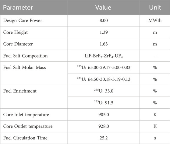
Table 1. The main reactor specifications of the MSRE.

Figure 1

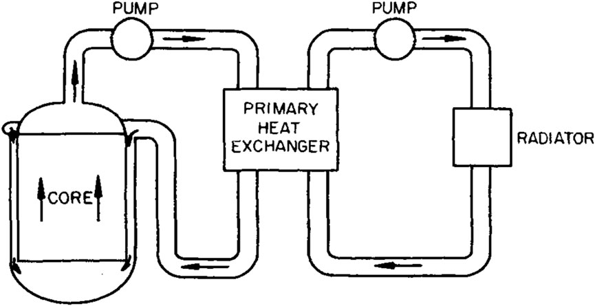
Figure 1. Layout of the primary and secondary loop of the MSRE (Kerlin et al., 1971a). The black arrows indicate the salt flow.

Figure 2

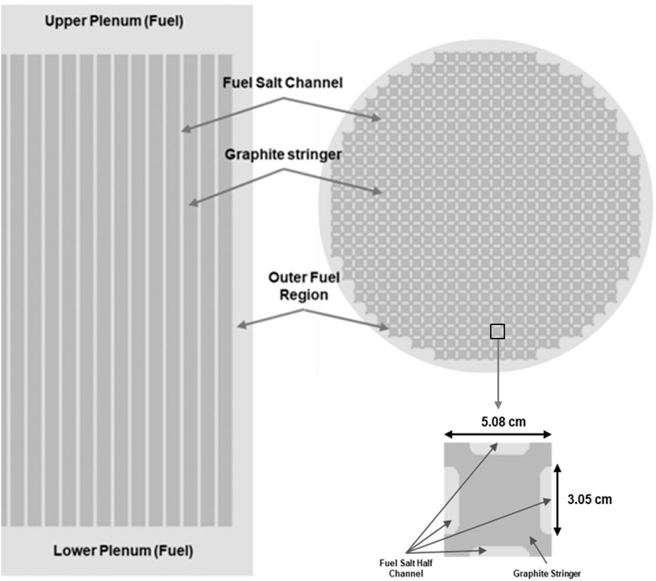
Figure 2. Axial (left) and radial (top right) views of the cross-section-generation model for the MSRE core assembly. The view of the graphite lattice (bottom right) shows the 4-halves fuel salt channels.

The MSRE’s liquid fuel salt was a FLiBe base salt bearing U and Zr, composed of LiF-BeF₂-ZrF₄-UF₄. The main fissile isotope was ²³⁵U, which was later replaced with ²³³U. The atomic fractions of the fuel salt isotopes are provided in Table 2 (Jaradat, 2021). The thermophysical properties of the fuel salt and solid moderator are provided in Table 3. This data was collected from several design and analysis reports of the MSRE (Gabbard, 1970; Compere et al., 1975). All the material properties considered in this model are temperature independent except for the fuel salt density $\rho$, which can be represented as a function of the fuel salt temperature $T$ as follows:

$\rho \left(T\right)=2263.0-0.4798\times \left(T-923.0\right).(23)$

Table 2

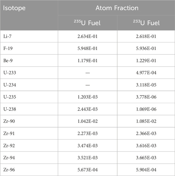
Table 2. MSRE fuel salt atomic concentration.

Table 3

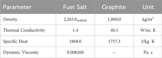
Table 3. Fuel salt and graphite thermophysical properties.

3.2 Developed models

The MSRE model was developed using a 2-D axisymmetric domain in R-Z coordinates for both the spatial-dynamics neutronics and thermal-hydraulics calculations based on a model of the MSRE previously developed by Idaho National Laboratory (Schunert et al., 2023; Jaradat and Ortensi, 2023). The spatial-dynamics neutronics model in Griffin uses the multigroup diffusion approximation of the linearized Boltzmann transport equation in a homogeneous medium. It accounts for the effect of the advection- and diffusion-driven drift of the DNPs and their decay in the outer loop by obtaining the DNP distributions from thermal-hydraulic calculations performed in Pronghorn using the porous media approximation.

A cut-through view of the reactor core vessel is provided on the left panel of Figure 3 (Robertson, 1965); it shows the graphite stringers with the fuel channels, the lower and upper plenum, the downcomer, and the reactor core vessel. On the right-hand side of Figure 3, the developed 2-D R-Z model for neutronics and thermal-hydraulics calculations is presented. This model includes the graphite-moderated core, lower and upper plenum, riser, fuel salt pump, primary heat exchanger, outer loop pipe, and the downcomer.

Figure 3

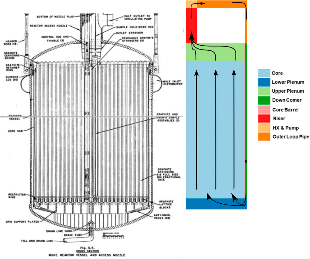
Figure 3. MSRE core on the left (Robertson, 1965) and 2-D R-Z model on the right.

The MSRE reactor geometry was simplified so the simulation and analysis could be efficient. The control rods and the outside regions of the active core, including the reactor vessel, the insulator, the gap between the reactor vessel and insulator, and the thermal shield, were not developed as part of the core configuration. The secondary loop was also not considered in the model. The temperature of the secondary side of the heat exchanger was set to a constant. The azimuthal symmetry of the MSRE model ignores some of the details of the real reactor system, but it preserves the important quantities of the core. The modeled core barrel has a radius of 0.70485 m, while the graphite-moderated core has a radius of 0.6914 m and a height of 1.6637 m. The lower plenum is 0.12954 m high, and the upper plenum is 0.21336 m high. The total salt volume in the reactor is 1.64 ${\text{m}}^3$.

The fuel’s total circulation time in the whole system is 25.2 s; the fuel transitions through the core, lower plenum, and upper plenum in 17 s. In the pump block, the fuel is accelerated by a uniformly distributed momentum source in the momentum equation with a total value equal to $1.15\times 10^8$ m/s². The volumes of the in-core and out-of-core regions reflect the volumes and circulation times reported in Refs. Ball and Kerlin (1965), Robertson (1965), Kerlin et al. (1971b). The fuel circulates upward through the core and is heated by the released fission power. At full power, the fuel temperature rises 23 K from the inlet to the outlet of the core. The fuel leaves the upper plenum through the riser, and heat $(q‴)$ is removed in the heat exchanger region according to the following relation:

$q‴=\alpha \left(T-T_{HX}\right),(24)$

where $\alpha$ is the volumetric heat transfer coefficient with a value of $2.22\times 10^7$ W/m³K, and $T_{HX}$ is the secondary side heat exchanger temperature, which is equal to 819.15 K. These values were selected to ensure the models matched the reported steady-state full-power fuel salt inlet temperature of 905 K.

A full 3D core model was developed for the MSRE using the Monte Carlo code OpenMC (Romano et al., 2015) to generate multigroup microscopic cross sections by accounting for the neutron spectral changes in the reactor core. This cross-section-generation model was adopted from Refs. Jaradat (2021), Jaradat and Sik Yang (2023). Additionally, the multigroup energy structure and the number of groups used to generate cross sections were selected based on a previous study (Jaradat, 2021; Jaradat and Sik Yang, 2023) that was performed to optimize the energy group structure and the number of groups. In this work, a 16-energy-group-structure was used to generate multigroup cross sections at several fuel salt and moderator temperatures using ENDF/B-VII.1 neutron data (Chadwick et al., 2011).

The fuel salt and graphite volume fractions in the reactor core region are 22.29% and 77.71%, respectively. This ratio is considered in obtaining cross-section homogenization and in the porous flow model implemented in Pronghorn. Additionally, the model considers the heat deposited in the solid graphite due to neutron thermalization and gamma heating. The considered value is $5.467\%$ of the total power produced in the reactor, which was calculated from previous OpenMC simulations presented in Jaradat (2021). The delayed neutron fraction and the decay constant for six delayed neutron groups of the ²³⁵U fuel and ²³³U fuel were also obtained from the same simulation, as reported in Table 4.

Table 4

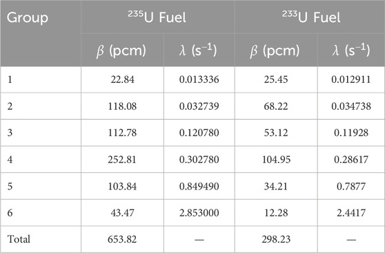
Table 4. MSRE delayed neutron precursor data.

3.3 Multiphysics coupling scheme

The multiphysics model of the MSRE was developed using the MOOSE MultiApps system, in which the coupling between the thermal-hydraulics solver and neutronics solvers is designed to allow for flexibility in exchanging problem variables using different neutronics models coupled to the same thermal model. Figure 4 shows the coupling scheme and the transferred parameters between the main application (Pronghorn) and the sub-applications (Griffin and Squirrel).

Figure 4

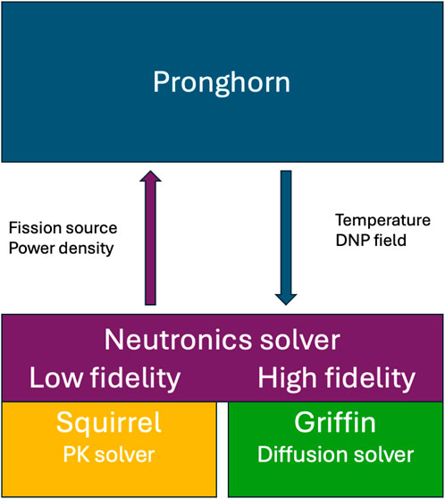
Figure 4. Coupling scheme between Pronghorn and the respective neutronics solver (Squirrel or Griffin).

Pronghorn is the main application, and it solves the Navier-Stokes equations, the DNP field for Griffin, and the reduced DNP field for Squirrel. Griffin provides the power density and fission source distributions to Pronghorn. The power density distribution is used to obtain fuel and moderator temperatures, density, pressure, and velocity fields. The fuel and moderator temperatures and the fuel density are used to update the cross sections for Griffin calculations. The fission source distribution is used in the calculation of the DNPs distribution to determine the delayed neutron source and reconstruct the total fission neutron source in the core region, considering their decay in the outer loop.

Squirrel relies on the initial neutron flux, power density, fission source density, and the kinetics parameters calculated by the steady-state Griffin simulation. Squirrel scales the power density and neutron flux during the transient calculations with a power amplitude function, where the steady-state power distribution or shape function is used throughout the entire transient simulation.

Since the neutronics solvers follow two different approaches, the key aspect of the coupling is to maintain the flexibility to swap each solver in each transient while maintaining the same Pronghorn simulation. This approach eliminates differences in the performance of the diffusion based neutronics solvers and the PK solver originating from thermal-hydraulics solutions.

In this work, we performed validation tests encompassing steady-state, pump start-up, pump coast-down, and natural circulation tests. The details of the coupling need to be different for each simulation. In this paper, the following three cases are evaluated:

1. Steady state: The eigenvalue problem is solved by Griffin, considering the steady-state diffusion equation with DNP concentration distributions based on the thermal field and DNP concentration distributions provided by Pronghorn, assuming a constant power level. Pronghorn solves a time-dependent problem until a steady-state solution is achieved at each Picard iteration.

2. Pump start-up and coast-down: The reference state is obtained at a very low power level and without fuel flow. Then, at each time step, new DNP concentration distributions are calculated by Pronghorn based on the pump head changes, and these distributions are used to reconstruct a new fission source and perform an eigenvalue calculation in Griffin to determine the reactivity losses due to fuel movement using Equation 4, while Squirrel solves Equation 16 to obtain the change in reactivity. During this simulation, Pronghorn solves a time-dependent problem, while the neutronics solve a steady-state problem. Since a constant low power level was maintained, thermal feedback is ignored, and the change in the eigenvalue can be attributed to the change in the DNP field.

3. Natural circulation test: Both neutronics codes and Pronghorn solve a time-dependent or transient problem starting from the initial steady-state solution to adapt to the power change. At each time step, Pronghorn exchanges the required variables with the neutronics solver to calculate the new power and temperature distributions.

4 Verification and validation tests

In this section, we provide a code-to-code verification between Griffin and Squirrel for transient analysis and validate these codes’ results against the experimental data of the MSRE. First, the steady-state solutions obtained from coupled Griffin-Pronghorn calculations are presented. Then, the results obtained with the multiphysics model employing Griffin and Squirrel are validated against the experimental measurements for the pump start-up and coast-down at zero power, along with natural circulation test results.

4.1 Steady-state results

In this sub-section, we provide the steady-state solutions of the MSRE model obtained from coupled Griffin and Pronghorn calculations for isothermal temperature coefficients and effective delayed neutron fractions of stationary and circulating fuels, along with steady-state distributions of the power, temperature, and DNP concentrations, which Squirrel needs to initiate coupled transient calculations.

Table 5 provides the calculated values of the isothermal temperature coefficients of the ²³⁵235U and ²³³U fuel salts. Due to the temperature dependency assumed for density in Equation 23, the temperature coefficients involve both the density and Doppler feedback. The isothermal temperature coefficient is calculated by globally varying the temperature in the reactor between 850 and 1000 K using Equation 5 and considering stationary fuel. The calculated values are also compared to values measured during operations of the MSRE, as reported in Prince et al. (1968).

Table 5

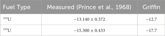
Table 5. Isothermal temperature coefficient (pcm/K) at 923 K for ²³⁵U and ²³³U fuels calculated by Griffin.

Figure 5 shows the reactor field variables obtained from coupled steady-state Griffin-Pronghorn calculations for power density, fuel salt temperature, and fuel salt velocity. The majority of the power is generated at the center of the active core region, while the outer core does not get heated. There are two apparent peaks in power density in the upper and lower plenum regions due to the massive increase in fuel salt volume and the absence of the graphite moderator in these regions.

Figure 5

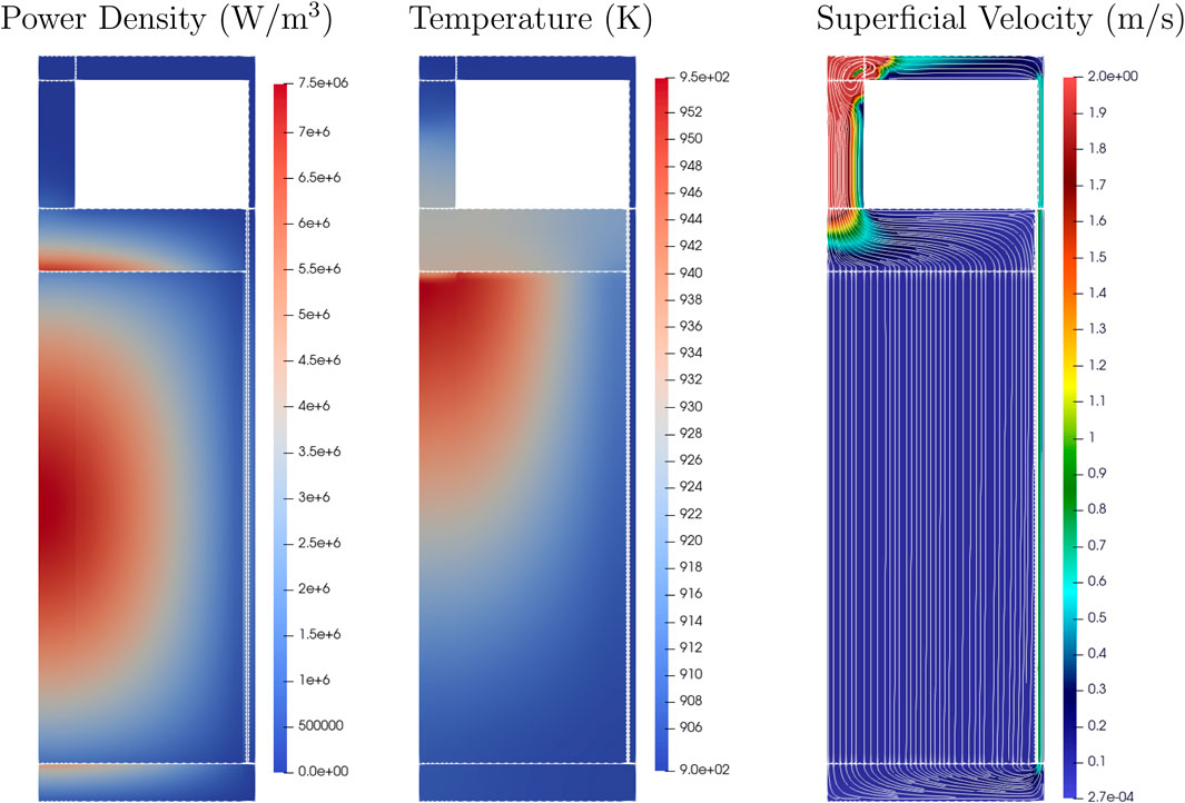
Figure 5. Steady-state field variables: power density, fuel salt temperature, and salt superficial velocity.

The middle plot of Figure 5 shows the fuel salt temperature distribution. The temperature distribution is skewed toward the top of the core, as expected, with an approximate maximum fuel temperature of 950 K at the top of the graphite block, close to the core’s center. In the upper plenum, colder salt from the outer regions of the core is drawn toward the riser located above the core’s center. There, the cooler salt mixes with the hotter salt from the core’s center, significantly reducing the fuel salt temperature.

The right plot of Figure 5 shows the fuel salt superficial velocity with streamlines indicating the fuel salt path. The salt enters the lower plenum from the downcomer and flows radially inward into the graphite block region, then flows upward without any lateral movement. In the upper plenum, the salt flows again radially inward toward the riser. In the riser, the flow rate is the highest since the cross-sectional area is the smallest. In the pump, the salt is forced to move through the elbow into the downcomer and back to the lower plenum again, with a total circulation time of 25.2 s.

For the flowing-fuel case, the DNPs are advected in the reactor core and the primary loop, resulting in the redistribution of the DNPs based on their half-lives, which leads to reactivity losses as DNPs decay in regions of lower importance. Outside of the active core, the importance of the DNPs is almost zero. Figure 6 depicts the distribution of the six groups of DNPs within the fuel salt for the reactor operating with ²³³U fuel salt. The longest-lived DNP group (Group 1) decays outside the active core region and peaks toward the top region of the core. The undecayed DNPs flow back into the core through the lower plenum, resulting in almost homogeneous mixing in the core. Groups 2 and 3 of the DNPs decay mostly in the outer region of the core, resulting in larger delayed neutron losses. For the shortest-lived group (Group 6), the DNPs decay at almost the same location as their initial position and peak toward the core center, resulting in smaller delayed neutron losses.

Figure 6

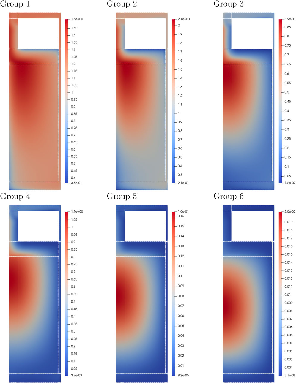
Figure 6. Steady-state DNP concentration (${\text{m}}^{-3}$) distributions in the MSRE ²³³U fuel salt. Group 1 at the top left is the longest lived, and Group 6 at the bottom right is the shortest lived.

Table 6 provides the effective delayed neutron fraction $\beta$ of stationary and flowing fuels, and the loss in effective delayed neutron fraction ${\beta }_{\mathit{loss}}$ for both ²³⁵U and ²³³U fuel salts. The reported MSRE values of the ²³⁵U fuel salt are from Prince et al. (1968); reactivity loss measurements were not reported for the ²³³U fuel salt. The effective delayed neutron fraction of the ²³⁵U fuel salt is 654 pcm, which is more than twice that of the ²³³U fuel salt, which is 298 pcm. The reactivity losses are almost 220 pcm for ²³⁵U fuel salt and 110 pcm for ²³³U fuel salt, with the relative loss in reactivity being similar for both fuels at around 35%. Squirrel-calculated reactivity losses due to fuel flow agree very well with Griffin values, with a difference of 3 pcm in both fuel cases. Also, both codes’ values agree well with the measured reactivity losses of 212 pcm for ²³⁵U fuel salt. For the stationary fuel case, Squirrel relies on the effective delayed neutron fraction calculated by Griffin.

Table 6

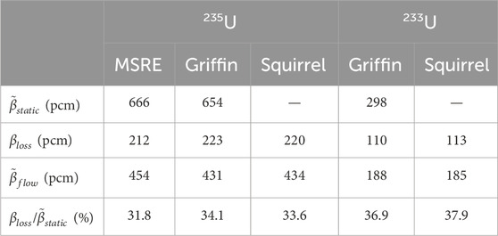
Table 6. Steady-state effective delayed neutron fraction of ²³⁵U and ²³³U fuels for stationary and flowing fuels.

4.2 Pump start-up and coast-down

In this section we discuss the results of the validation test against the experimental data of the pump start-up and coast-down tests. These tests were performed with ²³⁵U fuel salt at a low power level (zero power or cold conditions). A detailed description of the experimental setup of this transient can be found in Prince et al. (1968). The mass flow rate of the fuel salt was adjusted through the primary salt pump, which resulted in reactivity perturbations. These reactivity changes were compensated for by adjusting the control rod position to match positive or negative reactivity insertion and by maintaining the reactor at a constant low power level (around 10 W) throughout the test. Therefore, the temperature reactivity feedback could be neglected in the simulations. The reported position of the control rods represents the reactivity change due to DNP redistribution and decay with changes in the fuel salt flow rate.

During the pump start-up test, as the fuel salt mass flow rate started increasing, the DNPs flowed outside the active core region and decayed in regions of lower importance and in the outer loop, resulting in increased reactivity losses. In the pump start-up simulation, the pump force in the thermal hydraulics model was adjusted to achieve a fuel mass flow rate change from 0% to 100% in approximately 8 s, while in the pump coast-down simulation the pump force was adjusted to achieve a fuel mass flow rate change from 100% to 0% in approximately 20 s. The slower coast-down of the fuel flow can be explained by the hydraulic inertia that the system had at maximum flow rate. The measured and calculated mass flow rates for both test cases are displayed in Figure 7, along with the normalized pump force values used in Pronghorn.

Figure 7

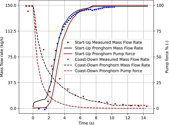
Figure 7. Relative pump force and mass flow rate evolution during the pump start-up and coast-down tests. The experimental data is from (Prince et al., 1968).

The estimated uncertainty for the measured reactivity considered in this work originates from the following parameters:

• Control rod position indicator: The uncertainty in the control rod position measurement during the zero power tests was estimated to be $\pm$ 0.01 inches.

• Integral worth curve: The stable period was determined by averaging the slopes of the two curves, which usually agreed within 2%.

• Fuel salt advection: Both the sensitivity of the rod-drop experiment and the fuel circulation indicate that the reactivity calculated from the integral worth curve may underestimate the value. For this reason, it is assumed that the uncertainty in the integral worth curve for the final loading is 2%.

Figures 8, 9 display, on the left-hand side, the experimental values of the reactivity along with simulation results for pump start-up and coast-down, respectively. During the pump start-up test, the redistribution and decay of the DNPs led to a maximum reactivity loss of 284 pcm after 13 s. As the undecayed DNPs reentered the active core region, the measured reactivity loss was reduced again and started oscillating at approximately 212 pcm until it reached steady-state conditions. During the pump coast-down test, the reactivity loss decreased as the fuel salt flow rate decreased due to the fact that the DNPs decay rate in the active core region increases. Finally, the reactivity loss reaches a zero value at zero-flow conditions, as the system returns to its initial state.

Figure 8

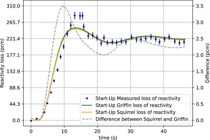
Figure 8. Reactivity loss during the pump start-up transient. The experimental data is from Prince et al. (1968).

Figure 9

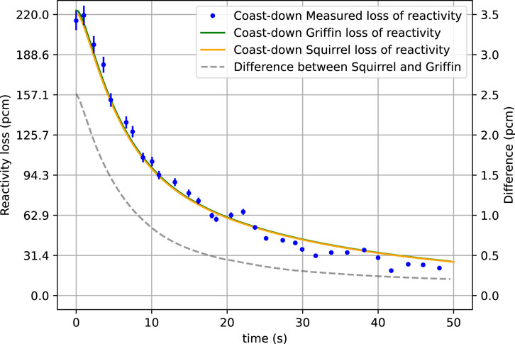
Figure 9. Reactivity loss during the pump coast-down transient. The experimental data is from Prince et al. (1968).

The simulation results of both codes show very good agreement for both pump tests. For the pump start-up test, both codes are in good agreement with the measured experimental values and captured the initial increase in reactivity loss and the final oscillation in reactivity loss, although they failed to capture the measured peak reactivity loss of 284 pcm by 34 pcm. The reason for this discrepancy is not fully understood, but it could be related to one or more of the following:

• Channel effect: The fuel channels are not resolved in the homogenized core model investigated here. The flow pattern in the fuel channels of the MSRE might cause a larger reactivity effect that the porous media approximation can not capture.

• Bubbles: Bubbles in the fuel salt have a negative reactivity effect, which is not considered in the current model. When the fuel starts to flow, bubbles are entrained from the cover gas in the reactor pump and advected through the primary circuit.

• Control rod servo: The flux servo controller kept the reactor critical during the experiment. Its precision during transients is not fully understood and it could have led to an overshooting after a fast change in reactivity.

For the pump coast-down test, both codes are in good agreement with the measured values for the entire period of the test. Additionally the difference in the simulation results obtained with Squirrel and Griffin is shown on the right axis of Figures 8, 9. The maximum difference between the two codes is 3.5 pcm for the pump start-up and 2.5 pcm for the coast-down. Since DNP advection has a minimal effect on the fundamental mode, good agreement between the codes is expected, as the assumption posed in Equation 9 is mostly fulfilled.

These transients increase our confidence that the circulation time and fuel volume are used properly, and they demonstrate that the neutronics solvers correctly evaluated the effect the shifted spatial distribution of the DNPs had on the reactivity.

In Figure 10, the density of the longest-lived DNP group (Group 1) is shown during the pump start-up test at different times up to 50 s. Initially, the DNP shape matches the fission source density in the core since there is no fuel flow. As the pump starts, the DNPs move upward into the riser (at approximately 10 s) and then down through the downcomer. At 20 s, the DNPs reenter the core from the bottom. This return of the DNPs into the core is responsible for the reduction in reactivity loss observed in Figure 8. The DNPs that are present at 30 s are advected out of the core, and at this time the returning DNPs have not yet reached the upper region of the core, leaving a region of lower DNP density in the middle of the reactor. At 50 s, the maximum DNP density is inside the core. Throughout the process, the DNPs are being mixed in the core.

Figure 10

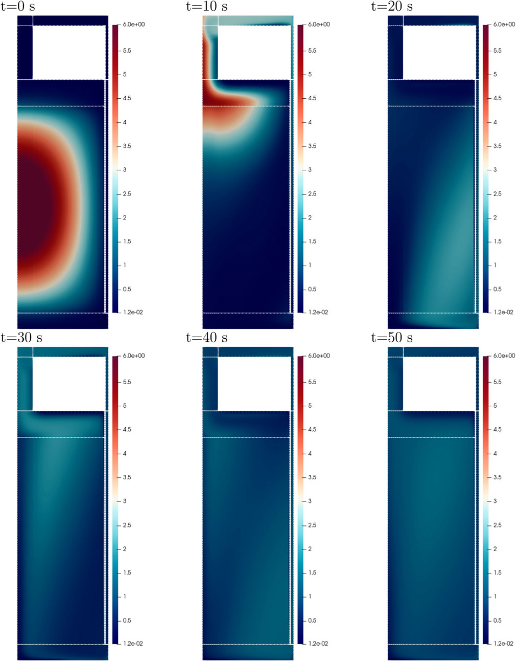
Figure 10. DNP concentration (${\text{m}}^{-3}$) distribution of Group 1 shown at different times during the pump start-up transient.

In Figure 11, the density of the longest-lived DNP group (Group 1) is shown during the pump coast-down test at different times up to 50 s. Initially, the DNPs are well mixed throughout the core. As the fuel flow is reduced (pump force reduced), more DNPs decay in the active core region, resulting in a decrease in reactivity losses. At 20 s, significantly fewer DNPs reenter the core from the bottom, clearly showing that fewer DNPs are advected through the outer core. At 50 s, the DNP shape matches the fission source density in the core. During the coast-down transient, the DNP density in the core increases steadily with minor oscillations.

Figure 11

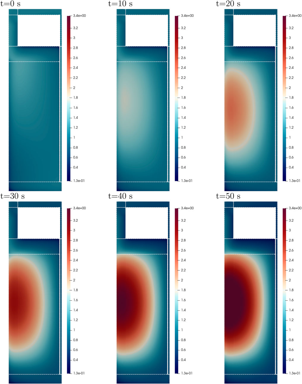
Figure 11. DNP concentration (${\text{m}}^{-3}$) distribution of Group 1 shown at different times during the pump coast-down transient.

4.3 Natural circulation test

In this test, the MSRE’s natural circulation was examined. The fuel pump was turned off and the fuel salt circulated through the system due to natural circulation. The main test characteristics can be summarized as follows:

• The reactor was operated with ²³³U fuel salt with the primary pump turned off.

• The regulating control rod remained in its initial position for the entire test.

• The reactor’s initial power was 4.1 kW, assuming the reactor was at equilibrium steady-state conditions.

• The fuel salt inlet temperature was slowly decreased by adjusting the flow rate on the secondary side.

• The uncertainty in the measured power signal was assumed to be 2%.

The reduction in the fuel salt temperature led to a positive reactivity insertion (due to the negative temperature coefficient); therefore, the power of the reactor increased as the temperature decreased. This increase in power and the resulting heating of the fuel increased the fuel temperature. The hotter fuel caused the power to stabilize at a new level. This process of reducing the fuel temperature was repeated several times, and multiple power plateaus were reached. The maximum power was 351 kW, and the final power was 324 kW. During the transient, the reactor power developed fully unprotected, with the control rod remaining in its initial position, and the reactor was fully driven by temperature feedback during the test. The effect of the DNP movement in the circulating fuel was minimal due to the very low fuel-flow rate (Rosenthal et al., 1969).

During the simulation, the inlet temperature was prescribed by adjusting the secondary temperature of the heat exchanger. The model used is not able to reproduce the reported fuel flow with natural circulation, most likely because it lacks the correct height difference between the core and the heat exchanger. Therefore, the mass flow rate was adjusted by changing the pump force in Pronghorn. The transient was induced by the prescribed change in inlet temperature and the adjustment of the pump force. With colder fuel entering the core, the power increases due to the positive temperature feedback. The increasing power heats up the core. The reactor reaches a steady power when the inlet temperature is kept constant, which happened multiple times during the transient.

Figure 12 shows the inlet mass flow rate and the inlet and outlet fuel temperatures alongside the measured inlet and outlet fuel temperatures reported in Rosenthal et al. (1969). Additionally, Figure 13 shows the reactor power evolution as measured and calculated by Griffin and Squirrel. The simulation results and the experimental data match reasonably well for the entire transient. Both the Griffin and Squirrel solutions match very well throughout the transient, with the maximum observed difference in total reactor power being 7.5 kW. The good agreement between the codes can be explained by the transient’s slow evolution and the minimal deformation of the fundamental mode. The largest difference in power measurements for the simulation and experimental data is seen at the beginning of the transient. After that, the power is well matched, resulting in good agreement between the simulated and experimental outlet temperatures. The assumption of thermal equilibrium conditions (steady state) at the beginning of the simulation may explain the temperature differences in the data for the beginning of the transient.

Figure 12

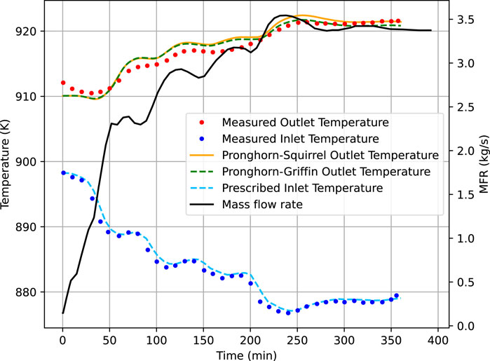
Figure 12. Mass flow rate and temperature evolution during the natural circulation test. The left axis shows inlet and outlet temperatures, and the right axis shows the mass flow rate. The experimental data is reported in Rosenthal et al. (1969).

Figure 13

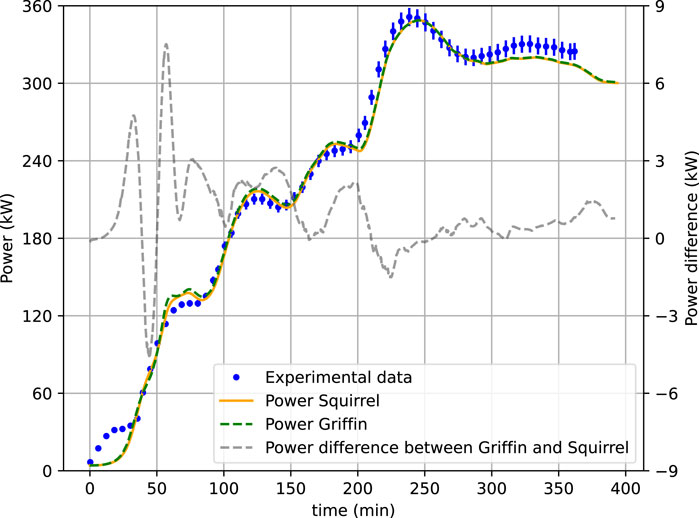
Figure 13. n values (left axis) of Griffin and Squirrel and the MSRE (Rosenthal et al., 1969) during the natural circulation test. The right axis shows the power difference between the codes.

Figure 14 shows the spatial power density in the reactor core at different times during the natural circulation test, as calculated by Griffin. Initially, the power density is low at 19.0 kW/m³; during the transient the power density increases up to 1.5 MW/m³ at 240 min. After that, it decreases slightly. At all times, the power density is highest in the center region of the core, and there is no measurable shift in the shape of the power density. Figure 15 shows the fuel salt temperature at different times during the natural circulation test. At the beginning of the transient, the inlet temperature increased up to 910 K, and it reached 960 K at the end of the transient. The difference in the simulated power obtained with Squirrel and Griffin is shown on the right axis of Figure 15. The maximum difference between the codes is 7.5 kW.

Figure 14

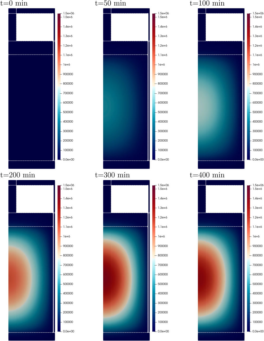
Figure 14. Power density (W ${\text{m}}^{-3}$) distribution shown at different times during the natural circulation test, as calculated by Griffin.

Figure 15

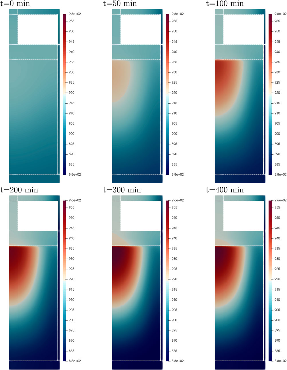
Figure 15. Fuel salt temperature (K) distribution shown at different times during the natural circulation test.

5 Summary

In this work, verification and validation test results were presented for the multiphysics modeling of the MSRE using coupled neutronics and thermal-hydraulics solvers developed under the MOOSE framework. The thermal-hydraulics calculations were performed with the Pronghorn code, which used an axisymmetric domain in R-Z coordinates with a porous media approximation. The neutronics calculations were performed with either the spatial neutron dynamics solver Griffin, which used an axisymmetric domain in R-Z coordinates with diffusion approximation in a homogenized domain, or the 0-D solver Squirrel with PK approximation. The developed model’s dimensions and its material’s thermophysical properties were obtained from the open literature, as were the experimental test data of the MSRE.

The models that were developed demonstrate the codes’ capability of modeling liquid flowing fuel and the resulting reactivity changes caused by the redistribution and decay of the DNPs. Both solution approaches were verified against each other and validated against the experimental data of the pump start-up, pump coast-down, and natural circulation tests. During the pump start-up and coast-down tests, both approaches predicted the reactivity loss resulting from fuel salt flow changes without thermal feedback effects. The test results of both approaches and their measured values show very good agreement. The maximum difference in reactivity loss between the two approaches is 3.5 pcm, indicating that the advection effects of the DNPs were captured accurately. For the natural circulation test, the fully coupled time evolution of the codes was tested. In this test, the inlet mass flow rate and inlet temperature were prescribed by adjusting the pump force and the secondary side inlet temperature to match the experimental data of the MSRE. Both approaches accurately predicted the power evolution during the test and captured the thermal feedback of the system.

A comparison of the results of the 0-D neutronics solver Squirrel and the spatial dynamics code Griffin, both coupled to the same thermal-hydraulics solver, showed that both codes yield similar results for the three tests, confirming that the codes capture the same physics qualitatively and quantitatively. This agreement in results suggests that the spatial weighting of DNPs used in the PK equation captures the physics to a degree similar to that of the spatial diffusion solver. While both neutronics solvers agreed on the presented transients, spatial dynamics offers a higher fidelity that the PK equation might not be able to capture. The PK equation is known to not being able to properly account for fast and local transients (Dulla et al., 2008). In a MSR these transients conditions might occur when:

• A fuel channel is blocked.

• The fuel salt is drained.

• Bubbles are formed locally and enter the core region.

• Over-cooled fuel enters the core.

• The reactor is over-fueled.

Future work will focus on testing spatial dynamics and PK codes on transients that are challenging to capture with the 0-D solver Squirrel, particularly fast and local transients. The separability assumption of flux shape and amplitude may not always hold for these scenarios. Additionally, strategies to mitigate the shortcomings of PK such as the improved quasi-static method in Griffin to update the shape function may help in the future.

Data availability statement

The raw data supporting the conclusions of this article will be made available by the authors, without undue reservation.

Author contributions

PP: Writing – review and editing, Writing – original draft. MJ: Writing – review and editing, Writing – original draft. MT: Writing – original draft, Writing – review and editing. RF: Writing – review and editing, Writing – original draft. SW: Writing – original draft, Writing – review and editing. JO: Writing – original draft, Writing – review and editing.

Funding

The author(s) declare that financial support was received for the research and/or publication of this article. The software development activities in this article were funded by the DOE Nuclear Energy Advanced Modeling and Simulation program. This research made use of the resources of the High Performance Computing Center at Idaho National Laboratory, which is supported by the Office of Nuclear Energy of the U.S. Department of Energy and the Nuclear Science User Facilities.

Conflict of interest

The authors declare that the research was conducted in the absence of any commercial or financial relationships that could be construed as a potential conflict of interest.

Generative AI statement

The author(s) declare that no Generative AI was used in the creation of this manuscript.

Publisher’s note

All claims expressed in this article are solely those of the authors and do not necessarily represent those of their affiliated organizations, or those of the publisher, the editors and the reviewers. Any product that may be evaluated in this article, or claim that may be made by its manufacturer, is not guaranteed or endorsed by the publisher.

Licenses and permissions

This manuscript has been authored by Battelle Energy Alliance, LLC/Idaho National Laboratory. The work was performed under Contract No. DE-AC07-05ID14517 with the U.S. Department of Energy. The United States Government retains and the publisher, by accepting the article for publication, acknowledges that the United States Government retains a non-exclusive, paid-up, irrevocable, world-wide license to publish or reproduce the published form of this manuscript, or allow others to do so, for United States Government purposes.

References

Aufiero, M., Brovchenko, M., Cammi, A., Clifford, I., Geoffroy, O., Heuer, D., et al. (2014). Calculating the effective delayed neutron fraction in the molten salt fast reactor: analytical, deterministic and Monte Carlo approaches. Ann. Nucl. Energy 65, 78–90. doi:10.1016/j.anucene.2013.10.015

CrossRef Full Text | Google Scholar

Ball, S., and Kerlin, T. (1965). Stability analysis of the molten-salt reactor experiment, Tech. rep. Oak Ridge, TN (United States): Oak Ridge National Lab.ORNL.

Google Scholar

Chadwick, M., Herman, M., Obložinský, P., Dunn, M., Danon, Y., Kahler, A., et al. (2011). ENDF/B-VII.1 nuclear data for science and technology: cross sections, covariances, fission product yields and decay data. Nucl. Data Sheets 112 (12), 2887–2996. doi:10.1016/j.nds.2011.11.002

CrossRef Full Text | Google Scholar

Compere, E., Kirslis, S., Bohlmann, E., Blankenship, F., and Grimes, W. (1975). Fission product behavior in the molten salt reactor experiment, Tech. rep. Oak Ridge, TN (United States): Oak Ridge National Lab.ORNL.

Google Scholar

Dulla, S., Mund, E. H., and Ravetto, P. (2008). The quasi-static method revisited. Prog. Nucl. Energy 50 (8), 908–920. doi:10.1016/j.pnucene.2008.04.009

CrossRef Full Text | Google Scholar

EVOL (2025). Available online at: https://cordis.europa.eu/project/id/249696/reporting.

Google Scholar

Fang, J., Hu, R., Gorman, M., Zou, L., Hu, G., and Hua, T. (2020). Sam enhancements and model developments for molten-salt-fueled reactors, Tech. rep. Argonne, IL (United States): Argonne National Lab.ANL.

Google Scholar

Fiorina, C., Clifford, I., Aufiero, M., and Mikityuk, K. (2015). Gen-foam: a novel openfoam® based multi-physics solver for 2d/3d transient analysis of nuclear reactors. Nucl. Eng. Des. 294, 24–37. doi:10.1016/j.nucengdes.2015.05.035

CrossRef Full Text | Google Scholar

Gabbard, C. (1970). “Reactor power measurement and heat transfer performance in the molten salt reactor experiment,”. Oak Ridge, TN (United States): Oak Ridge National Lab.ORNL.

Google Scholar

GeNFOAM (2025). Available online at: https://gitlab.com/foam-for-nuclear/GeN-Foam.

Google Scholar

Habtemariam, N., Fiorina, C., Lorenzi, S., and Cammi, A. (2024). On the need for multi-dimensional models for the safety analysis of (fast-spectrum) molten salt reactors. Ann. Nucl. Energy 197, 110237. doi:10.1016/j.anucene.2023.110237

CrossRef Full Text | Google Scholar

Haubenreich, P. N., and Engel, J. (1970). Experience with the molten-salt reactor experiment. Nucl. Appl. Technol. 8 (2), 118–136. doi:10.13182/nt8-2-118

CrossRef Full Text | Google Scholar

Hu, R., Zou, L., Hu, G., Nunez, D., Mui, T., and Fei, T. (2021). Sam theory manual, Tech. rep. Argonne, IL (United States): Argonne National Lab.ANL.

Google Scholar

Jaradat, M., Ortensi, J., and Yang, G. (2023). “Multiphysics analysis of the MSRE experiment using Griffin-Sam coupled code system,” in 2023 ANS winter conference and expo. Idaho Falls, ID: Idaho National Laboratory, INL/RPT-23-72875.

Google Scholar

Jaradat, M. K. (2021). Development of neutronics analysis capabilities for application of flowing fuel molten salt reactors. (PhD thesis). University of Michigan, Ann Arbor, MI, United States.

Google Scholar

Jaradat, M. K., Choi, N., and Abou-Jaoude, A. (2024). Verification of griffin-pronghorn-coupled multiphysics code system against cnrs molten salt reactor benchmark. Nucl. Sci. Eng. 198, 2403–2436. doi:10.1080/00295639.2024.2306702

CrossRef Full Text | Google Scholar

Jaradat, M. K., and Ortensi, J. (2023). Thermal spectrum molten salt-fueled reactor reference plant model. Idaho National Laboratory. INL/RPT-23-72875.

Google Scholar

Jaradat, M. K., and Sik Yang, W. (2023). An adaptive time-stepping control algorithm for molten salt reactor transient analyses. Ann. Nucl. Energy 190, 109880. doi:10.1016/j.anucene.2023.109880

CrossRef Full Text | Google Scholar

Kedl, R. (1970). “Fluid dynamic studies of the molten-salt reactor experiment (msre) core,”. Oak Ridge, TN (United States): Oak Ridge National Lab.ORNL.

Google Scholar

Kerlin, T., Ball, S., and Steffy, R. (1971a). Theoretical dynamics analysis of the molten-salt reactor experiment. Nucl. Technol. 10 (2), 118–132. doi:10.13182/nt71-a30920

CrossRef Full Text | Google Scholar

Kerlin, T., Ball, S., Steffy, R., and Buckner, M. (1971b). Experiences with dynamic testing methods at the molten-salt reactor experiment. Nucl. Technol. 10 (2), 103–117. doi:10.13182/nt71-a30919

CrossRef Full Text | Google Scholar

Kophaiza, J., Szieberth, M., Feher, S., Czifrus, S., and De Leege, P. F. (2004). Monte Carlo calculation of the effects of delayed neutron precursor transport in molten salt reactors. IL (United States): American Nuclear Society.

Google Scholar

Laureau, A., Rosier, E., Merle, E., Beils, S., Bruneau, O., Blanchon, J. C., et al. (2021). The LiCore power plant simulator of the molten salt fast reactor. EPJ Web Conf. 247, 06030. doi:10.1051/epjconf/202124706030

CrossRef Full Text | Google Scholar

Lindsay, A., Giudicelli, G., German, P., Peterson, J., Wang, Y., Freile, R., et al. (2023). Moose Navier–Stokes module. SoftwareX 23, 101503. doi:10.1016/j.softx.2023.101503

CrossRef Full Text | Google Scholar

Lindsay, A. D., Tano Retamales, M. E., Giudicelli, G. L., German, P., and Schunert, S. (2021). “Improvement of numerical methods in pronghorn,”. Idaho Falls, ID (United States): Idaho National Laboratory NL.

Google Scholar

Locatelli, G., Mancini, M., and Todeschini, N. (2013). Generation iv nuclear reactors: current status and future prospects. Energy Policy 61, 1503–1520. doi:10.1016/j.enpol.2013.06.101

CrossRef Full Text | Google Scholar

Mascaron, M., Le Meute, T., Martinet, J., Pascal, V., Bertrand, F., and Merle, E. (2023). “Study of the aramis molten salt reactor behavior during unprotected transients,” in ICAPP 2023-2023 international congress on advances in nuclear power plants, in conjunction with 38th korea atomic power annual conference (ICAPP 2023/KAP conference).

Google Scholar

Mattioli, A. S., Fiorina, C., Lorenzi, S., and Cammi, A. (2021). Derivation and implementation in openfoam of a point-kinetics model for molten salt reactors. Trans. Am. Nucl. Soc. 125 (1), 448–451. Available online at: https://hdl.handle.net/11311/1225555.

Google Scholar

Moukalled, F., Mangani, L., and Darwish, M. (2016). The finite volume method. Cham: Springer International Publishing, 103–135.

Google Scholar

Novak, A., Carlsen, R. W., Schunert, S., Balestra, P., Reger, D., Slaybaugh, R., et al. (2021). Pronghorn: a multidimensional coarse-mesh application for advanced reactor thermal hydraulics. Nucl. Technol. 207 (7), 1015–1046. doi:10.1080/00295450.2020.1825307

CrossRef Full Text | Google Scholar

Pfahl, P., Chambon, A., Groth-Jensen, J., and Lauritzen, B. (2025). Squirrel: a moose-based app for solving point kinetics in molten salt reactors. Nucl. Sci. Eng., 1–13. doi:10.1080/00295639.2025.2494182

CrossRef Full Text | Google Scholar

Prince, B., Ball, S., Engel, J., Haubenreich, P., and Kerlin, T. (1968). “Zero-power physics experiments on the molten-salt reactor experiment,”. Oak Ridge, TN (United States): Oak Ridge National Lab.ORNL.

Google Scholar

Robertson, R. C. (1965). “Msre design and operations report part 1 description of reactor design,”. Oak Ridge, TN (United States): Oak Ridge National Lab.ORNL.

Google Scholar

Romano, P. K., Horelik, N. E., Herman, B. R., Nelson, A. G., Forget, B., and Smith, K. (2015). Openmc: a state-of-the-art Monte Carlo code for research and development. Ann. Nucl. Energy 82, 90–97. doi:10.1016/j.anucene.2014.07.048

CrossRef Full Text | Google Scholar

Rosenthal, M., Briggs, R., and Kasten, P. (1969). “Molten-salt reactor program semiannual progress report for period ending february 28, 1969,”. Oak Ridge, TN (United States): Oak Ridge National Lab.ORNL.

Google Scholar

SAMOFAR (2025). Available online at: http://samofar.eu/.

Google Scholar

SAMOSAFER (2025). Available online at: https://samosafer.eu/.

Google Scholar

Schunert, S., Tano, M., and Jaradat, M. K. (2023). “Overlapping domain coupling of multidimensional and system codes in neams - pronghorn and sam,”. Idaho Falls, ID (United States): Idaho National Laboratory INL. doi:10.2172/1998551

CrossRef Full Text | Google Scholar

Serp, J., Allibert, M., Beneš, O., Delpech, S., Feynberg, O., Ghetta, V., et al. (2014). The molten salt reactor (msr) in generation iv: overview and perspectives. Prog. Nucl. Energy 77, 308–319. doi:10.1016/j.pnucene.2014.02.014

CrossRef Full Text | Google Scholar

Shi, J., and Fratoni, M. (2020). “Gen-foam model and benchmark of delayed neutron precursor drift in the molten salt reactor experiment,” in EPJ web of conferences (EDP Sciences).

Google Scholar

Wang, Y., Prince, Z. M., Park, H., Calvin, O. W., Choi, N., Jung, Y. S., et al. (2025). Griffin: a moose-based reactor physics application for multiphysics simulation of advanced nuclear reactors. Ann. Nucl. Energy 211, 110917. doi:10.1016/j.anucene.2024.110917

CrossRef Full Text | Google Scholar