 Jackson R. Harter
 Mark D. DeHart
- 1Reactor Physics and Shielding, Idaho National Laboratory, Idaho Falls, ID, United States
- 2Department of Nuclear Science and Engineering, Abilene Christian University, Abilene, TX, United States
The research presented in this article describes progress in applying stochastic methods, uncertainty quantification, parametric studies, and variance-based sensitivity analysis (also known as Sobol sensitivity analysis) to a full-core model of a nuclear thermal propulsion (NTP) system simulated via the radiation transport code Griffin to simulate neutronics. Our goal is to develop a reduced-order (surrogate) model that can be rapidly sampled with perturbations to multiple input parameters. In this NTP system, reactivity and power feedback affect the rotation of control drums (CDs), which is itself controlled by a hybrid proportional-integral-derivative (PID) controller actuated by the power demand and reactivity feedback from the numerical model. This model uses reactor kinetic feedback (mean generation time
1 Introduction
Supporting the development of space nuclear power for (1) nuclear fission power sources for spacecraft or lunar bases and for (2) spacecraft thrust is vital if humanity desires to regularly travel beyond the earth or moon (Buden, 2011). In terms of thrust, current chemical propulsion methods are limited by the amount of fuel they must carry, which restricts their operational ranges and efficiency. Nuclear power—particularly nuclear thermal propulsion (NTP)—offers a promising alternative by significantly enhancing the efficiency and capabilities of space missions. NTP affords a specific impulse
Idaho National Laboratory (INL) has been at the forefront of the development of advanced reactor simulation tools to model and analyze the behavior of NTP systems (DeHart et al., 2022). One decisive challenge in this area is the precise control of reactivity and power levels within the reactor core. In existing concepts (Venneri et al., 2016), this is accomplished via the rotation of control drums (CDs) to adjust the neutron flux and, hence, the reactor power. The control system for these CDs must respond dynamically to varying power demands and reactivity conditions that are influenced by the thermal and neutronic characteristics of the reactor. To address this, advanced control systems such as ones that utilize proportional-integral-derivative (PID) controllers are employed. These controllers require robust tuning and validation to handle the nonlinearities and uncertainties inherent in NTP operations (Labouré et al., 2023).
To advance the reliability and performance of NTP systems, uncertainty quantification (UQ) and sensitivity analysis (SA) must be performed. By enabling assessment of how uncertainties in input parameters propagate through the model to affect the outputs, UQ identifies the key parameters that influence system performance. Alternatively, SA aids in understanding the output’s dependency on input variations, as it is pivotal in optimizing control strategies and ensuring robust operation under varying conditions.
This work examines application of the Multiphysics Object-Oriented Simulation Environment (MOOSE) Stochastic Tools Module (STM) to the Griffin code (Wang et al., 2025; Slaughter et al., 2023) which was used to simulate a startup transient that was autonomously controlled with CDs through reactivity and power feedback via a PID controller. We investigated the effect of placing distributions on the PID control coefficients that affect power and reactivity. We explored the role that temperature changes play in NTP control as well as how CD movement is affected. We then developed a polynomial regression based surrogate model, using Latin Hypercube Sampling (McKay and Conover, 1979), of the NTP startup transient. This model can be rapidly sampled to yield statistical quantities at speeds orders of magnitude faster than running the training model, yet still generate very similar outcomes. Finally, we performed a variance-based sensitivity analysis (e.g., Sobol analysis), a global method, of the model in order to examine the variance of a quantity of interest (CD angle, or control signal) (a PID coefficient) based on the influences of the other uncertain parameters. It is imperative to note that this work is a proof-of-principle effort to exercise the stochastic tools module in MOOSE on a complex, 3D simulation, the startup sequence of a nuclear thermal propulsion module. The number of perturbed parameters are low compared to other conventional studies. It is our intent to apply the knowledge gained from this study to even more complex, coupled multiphysics problems.
In Section 2, we describe the neutronics NTP model. Section 3 describes the stochastic methods and shows the results for each case. Finally, we present our concluding remarks in Section 4.
2 Nuclear thermal propulsion model
2.1 Nuclear thermal propulsion model
The development and optimization of NTP systems requires a comprehensive understanding of the reactor’s dynamic behavior under various operating conditions. In the present work, UQ and SA were performed on an existing reactor model for NTP in a transient setting. This model was taken from a previous study by Labouré et al. (2023). The initial conditions were generated using point reactor kinetics and an eigenvalue calculation for a power increase transient; the transient simulates an initial burn and constant power throttle. The original model consisted of neutronics, heat conduction, and thermal hydraulic physics, but the present work examines only neutronic behavior. This focus enables detailed investigation of the neutronic response and control mechanisms, without the added complexity of thermal and hydraulic feedback. Isolating the neutronics component allows us to more effectively apply stochastic methods and SA to identify the key factors influencing reactor performance during transient operations. Two different device simulations were used to determine the control of the reactor. The first uses power feedback expressly to provide control drum (CD) rotation. As power demand increases, CDs turn to insert reactivity and raise the power. This model meets the demand, but undershoots the initial power demand. The hybrid controller uses both reactivity and power feedback to set the rotation angle of the CDs. It is much better suited to the task, meeting the initial power demand for the transient and matching it throughout.
2.1.1 Neutronics model
The full NTP simulation is a multiphysics model that incorporates neutronics, heat conduction, and thermal hydraulic physics modeled via Griffin/BISON/THM (Wang et al., 2025; Williamson et al., 2012; Hansel et al., 2024). The model considered in this study is a standalone neutronics model with no temperature or thermal fluids feedback; Figure 1 shows the full core and assembly model, respectively, developed with the Monte Carlo code Serpent2 (Leppänen, 2007). The cross sections for this model were generated using Serpent2, as was the full-core heterogeneous model described in (Labouré et al., 2023). The temperature range for the fuel was extended from a maximum of 2275 K–3175 K, and a reflector temperature of 300 K (conservatively simulating the boundaries of outer space) was added. Thus, the full range of temperatures is (1) fuel: 475–3175 K, (2) moderator: 150–705 K, and (3) reflector: 300 K. The moderator temperature range and CD angle
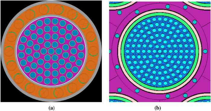
Figure 1. Overview of the core and assembly geometry in Serpent. Source: Labouré et al. (2023). (a) Radial view. (b) Zoom-in on assembly.
The neutronics model contains a total of 112 state points, each obtained by a Serpent2 calculation, performed with 2,000 cycles of
This model used constant temperatures during steady state and transient simulations. The energy group structure for the model was also kept the same. Instead of transport, diffusion was used in order to reduce the computational time and memory requirements. We used the continuous finite element method (CFEM) in concurrence with diffusion.
Also, combining the continuous finite element method with diffusion enables us to take advantage of the improved quasi-static (IQS) method to provide point kinetics parameters. IQS is a transient spatial kinetics method where space and time components of the neutron flux are represented by a time-dependent amplitude and a time-, space-, and energy-dependent shape (Prince and Ragusa, 2019). With this method, one can solve for kinetics parameters—reactivity
Existing models for the NTP steady state were used, consisting of two input files: (1) to solve for the adjoint solution, obtaining reactor physics kinetic parameters and (2) a forward solve to obtain a temperature distribution. A steady-state power of 500 kWth served as an arbitrary set point for simulating reactor startup. The converged steady-state solutions are used as initial conditions for the Griffin transient simulation; MOOSE has a restart system which enables this capability, the output solution is read in as an initial condition. Figure 2 is a transparency of the full core mesh used in the neutronics simulation. An important aspect to consider, and which was first addressed in Labouré et al. (2023), is that the adjoint calculation (required for the hybrid PID control) relies on an initial condition of temperature for the fuel and moderator regions [Note that the adjoint solution is used to compute time-dependent kinetics parameters]. However, since computation of these parameters ignores changes in temperature, the PID controller might compute a signal based on potentially inaccurate kinetics parameters (Labouré et al., 2023). In future work, a method of addressing this issue should be developed to ensure accuracy.
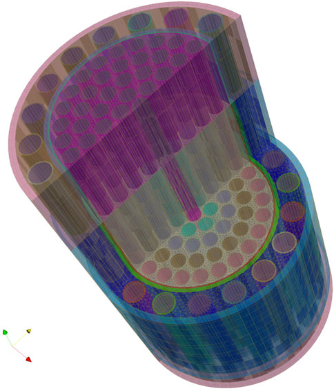
Figure 2. Full-core neutronics mesh.
2.1.2 Demanded and measured power
Labouré et al. used an exponential ramp-up power benchmark in their research (detailed in (Labouré et al., 2023)). We followed the same approach by using an initial power set point of
where
2.1.3 Power-driven PID control
Power-driven PID control is the simplest control strategy, relying on power demand
The measured power is computed by the 3D full-core neutronics model. The rotation angle of the drums is described by:
where
where
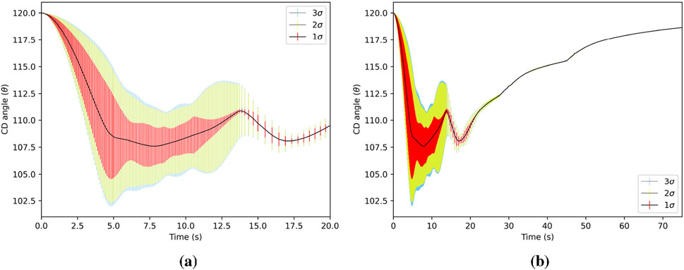
Figure 3. Mean value of total CD angle (standard deviation is shown as vertical bars) out to 3σ for as a function of time. The 3σ encompasses the other intervals. The CD angle has the largest σ during the initialization, when reactivity is changing fast to meet the power demand. The total CD angle is the actual angle of the drum. (a) CD angle for 0 < t ≤ 20s. (b) CD angle for 0 < t ≤ 75s.
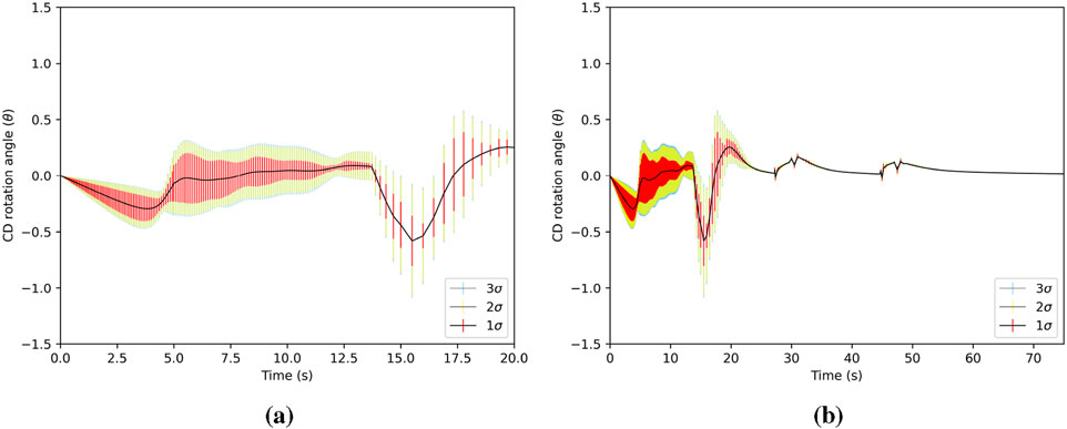
Figure 4. Mean value of CD angle of rotation (standard deviation is shown as vertical bars) out to 3σ as a function of time. The rotation angle is the increment of rotation at each time step, added to the total drum angle. (a) CD rotation angle for 0 < t ≤ 20s. (b) CD rotation angle for 0 < t ≤ 75s.
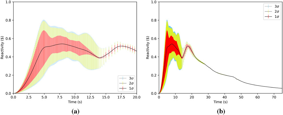
Figure 5. Mean value of reactivity (standard deviation is shown as vertical bars) out to 3σ as a function of time. Reactivity changes the most during the simulation initialization in order to meet the power demand. (a) Reactivity for 0 < t ≤ 20s. (b) Reactivity for 0 < t ≤ 75s.
2.1.4 Hybrid feedback controlled model
Labouré et al. combined power-driven PID control with reactivity-driven PID control. Whereas the power-driven PID performed well in the later stages of the transient but poorly in the initial stage, the reactivity-driven PID performed well in the early stages but not the later ones. This led to the development of hybrid PID control, which combines power and reactivity (and kinetics data) [see Figure 6 for an illustration].
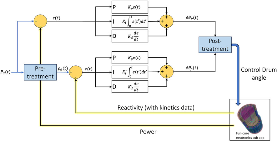
Figure 6. Diagram of the hybrid PID controller, showing feedback between the reactivity, power, and CD movement.
The reactivity error signal is defined as:
where
where
where
where
Results for the hybrid PID controller can be found in (Labouré et al., 2023). For the purpose of applying stochastic methods, we found that the hybrid PID controller performed well and is an ideal candidate for this work.
3 Stochastic methods and analysis approach
The objective of this work is to provide a reduced-order (surrogate) model of a neutronics system that can control an NTP module by automatically regulating CD movement based on coupled feedback effects.
The desire to rapidly sample a surrogate, analyze sensitive parameters, perturb various quantities of interest (QoIs), and predict NTP behavior motivated the coupling of MOOSE’s STM (Slaughter et al., 2023) to the Griffin code. UQ and SA methods have only recently become mature enough to handle large (
In a simulation without STM (referred to hereafter as the “nominal” simulation, which is the case where the modeling parameters are their base [non-perturbed] value), the power or hybrid PID controller input (the main application [master app]) instantiates the Griffin transient simulation as a sub-application (sub-app), and the MultiApp system transfers governs the quantities passed back and forth between the master and sub-app. The master app sends the CD angle to the Griffin sub-app and receives the measured power
When the Griffin neutronic simulation is coupled with the STM framework (in the sense of the MultiApp system in MOOSE), the STM input becomes the master app, the PID input becomes a sub-app, and the Griffin transient becomes a sub-sub-app (e.g., parent, child, grandchild). This is illustrated in Figure 7. The focus of our investigation is to understand the uncertainty and sensitivity of the PID controller, and how that uncertainty propagates through and affects the motion of the CDs, in turn affecting power and reactivity. We designed a suite of STM inputs to (1) learn how to apply these tools to large and complex simulations, (2) develop a surrogate model for use in a non-nuclear advanced controls testbed reactor, and (3) create a UQ/SA methodology for future applications.
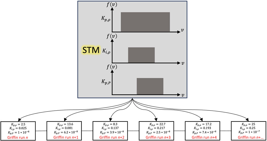
Figure 7. The STM input commands the flow of information to and from all the sub-apps used in the overall simulation process. In our application, uniform distributions were applied to parameters of interest and, depending on the number of samples desired, placed into subintervals. As the master application initiates, STM instantiates N instances of the Griffin base simulation. Each of these N instances has unique PID coefficient values. The base simulation transient is completed N times, and once these sets are finished their data are passed back to STM so statistical quantities such as the mean and standard deviation can be computed. This figure only shows how six distributions of PID coefficients can be used. STM is flexible, and those distributions can be changed out, or other parameter distributions can be included.
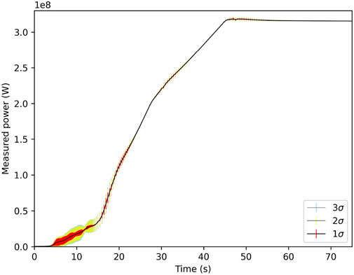
Figure 8. Measured power mean and standard deviation out to 3
In order to efficiently capture the dynamics of this system, the STM suite was chosen with regards to it being a MOOSE application, which allows for seamless integration with other MOOSE applications (just one of the benefits to using MOOSE-based simulation tools). Other stochastic packages such as RAVEN (Alfonsi et al., 2020) and Dakota (Adams et al., 2025) exist, but STM was selected exactly because it can integrate easily with other MOOSE-based codes. The stochastic approach is necessary to understand the influence of uncertainty in PID control parameters; physical components have an inherent uncertainty, whether it be through manufacturing defects, environmental effects, or user error. It is our task to understand just how important these uncertainties are.
We developed a protocol for applying stochastic methods to Griffin simulations, and ultimately we developed a surrogate model of an NTP module:
The total computational overhead of running
In an STM input, we specified the number of processes allocated to one sample. After brief trial and error, we deemed 192 processes per sample to be efficient. This is equal to four nodes (each node having 48 processes) on the Sawtooth High Performance Computing Cluster (HPCC) at INL, and it takes approximately 5.5 h to complete one transient hybrid PID-controlled neutronics simulation. We take advantage of parallel computing and require the STM simulation to run in batches. We selected 1,920 total processes and so ran them in groups of 10 (e.g., every 5.5 h, 10 samples were completed at a rate of approximately
3.1 Parameter sampling study
To understand how STM functions with Griffin as a sub-app, simple STM inputs were designed to observe how stochastic methods affect the QoI’s of CD angle, reactivity, and power. We used Latin Hypercube Sampling for both models. The PID controls employed multiple logic functions informed by desired power set points to control the neutronics simulation. The CD rotation is determined by a linear combination function with three coefficients that act on error functions for the proportional, integral, and derivative values. This phase of investigation is essentially a parameter study; the ranges of values chosen for the PID coefficients reflect this. In the following section, uniform distributions are placed on various constant of the PID controller:
3.1.1 Power PID statistical model
For the power feedback PID controller, our model applied a uniform distribution on the proportional constant
3.1.2 Hybrid PID statistical model
We switched from the power feedback model to the hybrid feedback model, which uses kinetic parameters (
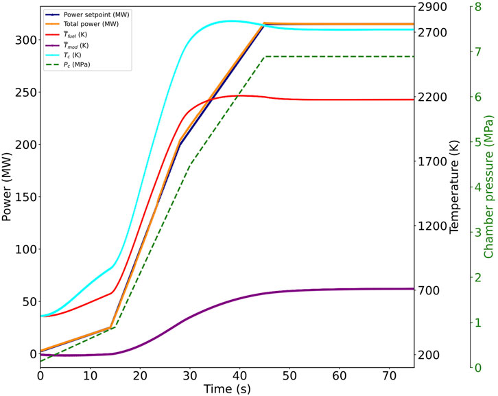
Figure 9. Evolution of power, temperature, and chamber pressure with a hybrid PID controller for the startup transient (Labouré et al., 2023).
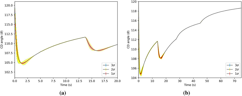
Figure 10. CD angle (standard deviation is shown as vertical bars). The CD angle has the largest standard deviation during the initialization, when reactivity is changing rapidly to meet the power demand. The total CD angle is the actual angle of the drum. (a) CD angle for 0 < t ≤ 20s. (b) CD angle for 0 < t ≤ 75s.
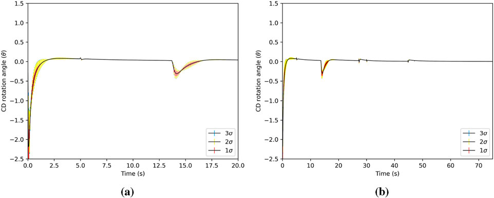
Figure 11. CD rotation angle (standard deviation is shown with vertical bars). The rotation angle is the increment of rotation at each time step, added to the total drum angle. (a) CD rotation angle for 0 < t ≤ 20s. (b) CD rotation angle for 0 < t ≤ 75s.
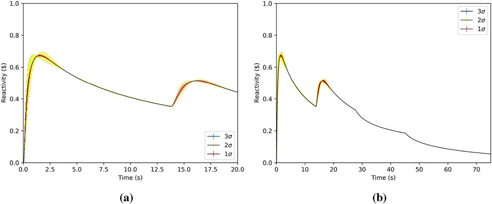
Figure 12. Reactivity (standard deviation is shown as vertical bars) as a function of time. Reactivity changes the most during the simulation initialization in order to meet the power demand. (a) Reactivity for 0 < t ≤ 20s. (b) Reactivity for 0 < t ≤ 75s.
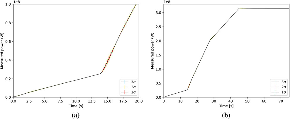
Figure 13. Power (standard deviation is shown as vertical bars) as a function of time. (a) Power for 0 < t ≤ 20s. (b) Power for 0 < t ≤ 75s.
It is clear in comparing the two controllers that the hybrid PID controller outperforms the power-driven PID controller. The fact that we generate better statistics with the hybrid PID is attributed to the superior control it affords by using both reactivity and power feedback. Even though the statistical error decreases as
3.2 Polynomial regression surrogate
In this study, we developed a polynomial regression surrogate as a reduced order representation of the time-dependent Griffin model. The polynomial regression surrogate is a full multidimensional polynomial expansion with all the cross terms, and with the number of dimensions being described by the number of distributions we use.
We used polynomials of order 4 in combination with an ordinary least-squares-type regression. Typically, a higher-order polynomial can fit the training data better, but it can also lead to overfitting, where the model captures noise instead of the underlying trend. Conversely, a lower-order polynomial may underfit the data, not capturing the complexity of the relationship. A polynomial order refinement study was not performed for this case; the selection of polynomial order 4 was an arbitrary choice for this model. However, future work could entail an order refinement study, in which regression surrogate models are tested for accuracy by varying polynomial order (Mukhtar et al., 2023; Zhao et al., 2022).
The problem setup is similar to that in the parameter sampling study, in that we use the same uniform distributions on the variables we know to be uncertain. The additional input directs the stochastic tools to train a surrogate model for the output we are interested in: CD angle, CD rotation angle, reactivity, and reactor power. This creates a library that can be sampled using a separate input file, can change the bounds of the uniform distribution (as long as they are within the original set [note that extrapolation is not recommended and accurate results not guaranteed]), and are sampled at rates orders of magnitude faster to give accurate results.
We compared the results of the training model against those of the surrogate. The training model took approximately 96 h to run on 60 Sawtooth nodes, using 150 samples to generate a training set. This amount of samples was sufficient to capture a range of one order of magnitude for each of the PID parameters; a larger range and number of parameters would merit an increase in the number of samples taken. The surrogate model sampling times are reported in Table 1. In general, the surrogate model can be sampled rapidly with little loss of accuracy in comparison to the training model.
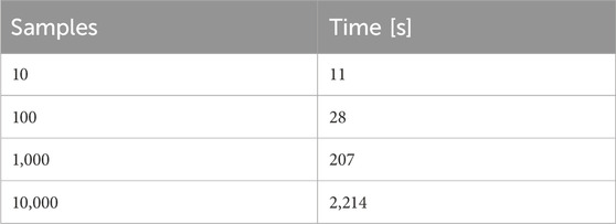
Table 1. Surrogate sample sizes and times.
We compared various surrogate sample sizes (10, 100, 1,000, and 10,000 samples) versus the training set (150 samples), and reported
where
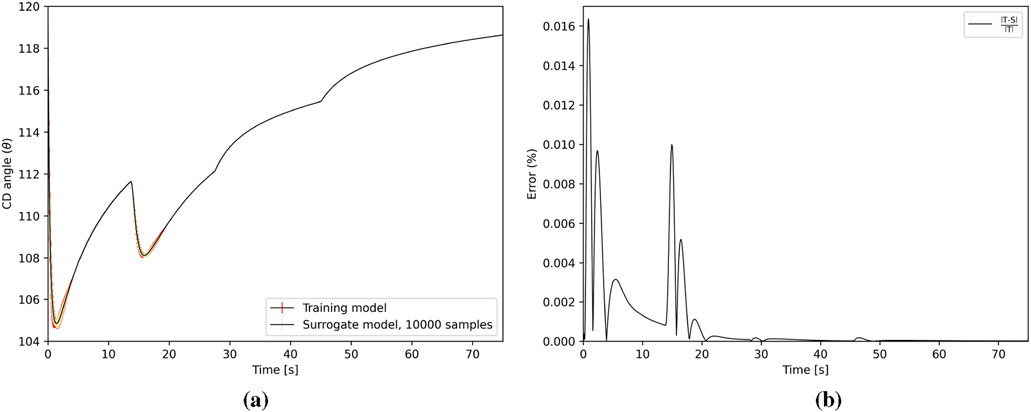
Figure 14. CD angle
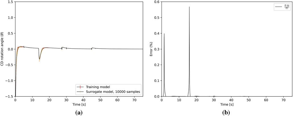
Figure 15. CD rotation angle
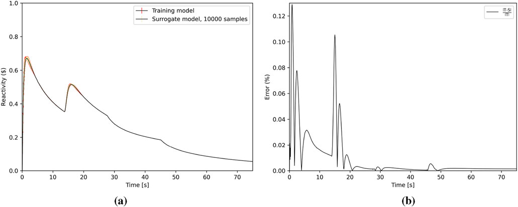
Figure 16. Reactivity
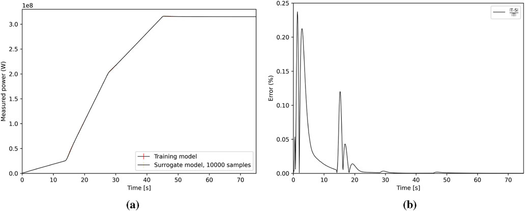
Figure 17. Power
The standard error (SE, the relative error in this study), in the standard deviation decreases monotonically as the number of samples increase, shown in Figure 18 and calculated with the relation in Equation 2 using the total number of samples
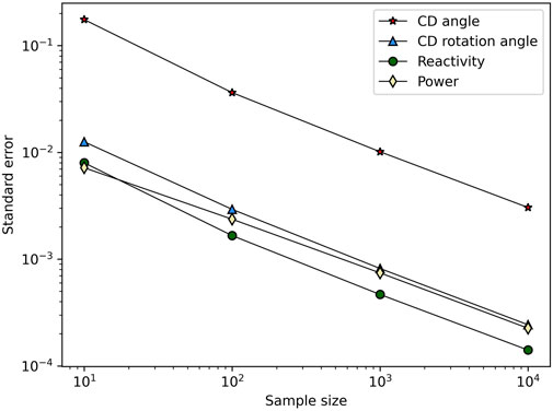
Figure 18. Standard error for QoIs in the surrogate model. The standard error in power was normalized to the mean of the power.
3.3 Variance-based (sobol) sensitivity analysis
The Sobol sampling scheme consists of using a sample and re-sample matrix to create a series of matrices that can be used to compute first-order, second-order, and total-effect sensitivity indices. We restrict our analysis to first-order effects in this study. The Sobol method was chosen as the primary approach to quantify how input uncertainties impact the variation in the key QoI’s; this method decomposes the variance of model outputs into contributions from each uncertain input and their interactions, offering a robust measure of how uncertainties propagate through complex systems (Saltelli, 2002).
We perform Sobol analysis by evaluating the surrogate model. The reason we choose to evaluate the surrogate model rather than the stochastic model in the previous section is because the hundreds of thousands of transient simulation runs would be computationally intractable; leveraging the efficiency of the surrogate, it is much easier to navigate the parameter space. The surrogate-based sensitivity analysis is implemented in the STM input file, very similar to the power and hybrid PID methodology.
The first order indices are the portion of the variance in the QoI (e.g.,
First-order Sobol indices were computed using 50,000 evaluations of polynomial regression surrogate models trained on the selected uncertain parameters. The resulting time-resolved indices illustrate how variations in PID coefficients influence system behavior throughout the startup transient. This study is one of few transient, three-dimensional simulations of a complex system model (Guo et al., 2023). Our goal in applying Sobol sensitivity analysis is to understand the sensitivity of the QoI during the transient; how the sensitivities change over the duration.
The results in Figure 19 are represented as the evolution of first-order Sobol indices over time for CD angle (Figure 19a) and integrated power (Figure 19a). The focus on first-order indices allows for the segregation of each parameter’s contribution to output variance without uniting interaction terms. In Figure 19a, the heatmap shows the normalized first-order Sobol index for the CD angle. The prominent vertical bars in Figure 19a correspond to the CD angle error in Figure 14b; these correspond to regions of rapid change in the transient where quick movement of CDs occurs–an inflection point, or rapid change in slope. A similar, more subtle effect is shown in Figure 19b. Though total Sobol indices capture both the main effects and interactions of QoIs, term these were excluded to streamline the analysis.
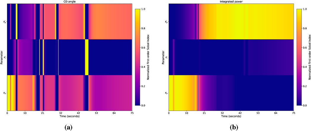
Figure 19. Time-resolved first-order Sobol indices for control drum angle and integrated power, showing the relative influence of PID uncertainties on the CD angle over time. The power coefficients (
4 Conclusion
Application of stochastic methods to Griffin simulations has proven successful in determining the specific parameters to which hybrid PID controllers are sensitive. Placing uniform distributions on the coefficient parameters and extracting statistical quantities of mean and standard deviation show how sensitive the PID controller is to subtle changes. We restricted our application of STM to a neutronics simulation as a first trial of stochastic methods on transient reactor physics simulation. In the future, we envision further multiphysics coupling, to heat conduction, thermal hydraulics, or heat pipes. This work was an initial study to test effectiveness.
Using a reduced-order model to simulate reactor startup affords many potential benefits, enabling rapid throughput analyses of different parameter variations so as to determine the “best fit” values for achieving precision startup control. Initially, we planned to use polynomial chaos expansions (PCEs) to develop the surrogate model, as the authors are experienced in using this method. However, at this stage of STM development, the PCE method cannot generate a time-dependent surrogate. The advantage of PCEs is that the quadrature-based sampling uses fewer samples than Monte Carlo or Latin Hypercube Sampling, for the same accuracy.
An area of concern in practical application of this method is the hybrid approach itself, which uses power and kinetic feedback to control the startup sequence. The terms we use for the feedback (
Data availability statement
The raw data supporting the conclusions of this article will be made available by the authors, without undue reservation.
Author contributions
JH: Visualization, Formal Analysis, Validation, Data curation, Conceptualization, Writing – review and editing, Software, Writing – original draft, Investigation, Methodology. MD: Supervision, Project administration, Funding acquisition, Writing – original draft, Resources.
Funding
The author(s) declare that financial support was received for the research and/or publication of this article. This manuscript has been authored by Battelle Energy Alliance, LLC under contract no.∼DE-AC07-05ID14517 with the U.S. Department of Energy, and this contract was funded by NASA’s Space Nuclear Propulsion (SNP) project within the NASA Space Technology Mission Directorate (STMD).
Acknowledgments
The authors thank Peter German for his guidance and invaluable discussions, and also thank Wafaa Osman for help with postprocessing scripting. This research made use of Idaho National Laboratory’s High Performance Computing systems located at the Collaborative Computing Center and supported by the Office of Nuclear Energy of the U.S. Department of Energy and the Nuclear Science User Facilities under contract no. DE-AC07-05ID14517.
Conflict of interest
The authors declare that the research was conducted in the absence of any commercial or financial relationships that could be construed as a potential conflict of interest.
The author(s) declared that they were an editorial board member of Frontiers, at the time of submission. This had no impact on the peer review process and the final decision.
Generative AI statement
The author(s) declare that no Generative AI was used in the creation of this manuscript.
Any alternative text (alt text) provided alongside figures in this article has been generated by Frontiers with the support of artificial intelligence and reasonable efforts have been made to ensure accuracy, including review by the authors wherever possible. If you identify any issues, please contact us.
Publisher’s note
All claims expressed in this article are solely those of the authors and do not necessarily represent those of their affiliated organizations, or those of the publisher, the editors and the reviewers. Any product that may be evaluated in this article, or claim that may be made by its manufacturer, is not guaranteed or endorsed by the publisher.
Licenses and permissions
This manuscript has been authored by Battelle Energy Alliance, LLC under contract no. DE-AC07-05ID14517 with the U.S. Department of Energy. The U.S. Government retains and the publisher, by accepting the article for publication, acknowledges that the U.S. Government retains a nonexclusive, paid-up, irrevocable, world-wide license to publish or reproduce the published form of this manuscript, or allow others to do so, for U.S. Government purposes.
References
Adams, B. M., Bohnhoff, W. J., Dalbey, K. R., Ebeida, M. S., Eddy, J. P., Eldred, M. S., et al. (2025). Dakota 6.21.0 documentation. Albuquerque, NM: Sandia National Laboratory.
Alfonsi, A., Rabiti, C., Mandelli, D., Cogliati, J., Wang, C., Talbot, P. W., et al. (2020). RAVEN theory manual. Idaho Falls, ID: Idaho National Laboratory. Technical report.
Cebollada, S., Payá, L., Flores, M., Peidró, A., and Reinoso, O. (2021). A state-of-the-art review on mobile robotics tasks using artificial intelligence and visual data. Expert Syst. Appl. 167, 114195. doi:10.1016/j.eswa.2020.114195
DeHart, M. D., Schunert, S., and Labouré, V. M. (2022). “Nuclear thermal propulsion,” in Nuclear reactors - spacecraft propulsion, research reactors, and reactor analysis topics. Editor C. L. Pope (United Kingdom: IntechOpen). Available online at: https://www.intechopen.com/chapters/103895.
Fan, T., Liu, L., Yue, Y., Chen, J., Wang, C., Yu, Q., et al. (2025). Truncated proximal policy optimization. Available online at: https://arxiv.org/abs/2506.15050.
Farcas, I., Merlo, G., and Jenko, F. (2022). A general framework for quantifying uncertainty at scale. Commun. Eng. 1, 43. doi:10.1038/s44172-022-00045-0
Guo, H., andXiaolong Fu, X. Z., Zhu, Y., and Rabczuk, T. (2023). Physics-informed deep learning for three-dimensional transient heat transfer analysis of functionally graded materials. Comput. Mech. 72, 513–524. doi:10.1007/s00466-023-02287-x
Hansel, J., Andrs, D., Charlot, L., and Giudicelli, G. (2024). The MOOSE thermal hydraulics module. J. Open Source Softw. 9, 6146. doi:10.21105/joss.06146
Labouré, V., Schunert, S., Terlizzi, S., Prince, Z., Ortensi, J., Lin, C.-S., et al. (2023). Automated power-following control for nuclear thermal propulsion startup and shutdown using MOOSE-based applications. Prog. Nucl. Energy 161, 104710. doi:10.1016/j.pnucene.2023.104710
Leppänen, J. (2007). Development of a new Monte Carlo reactor physics code. (Ph.D. thesis). Helsinki University of Technology.
McKay, R. J. B. M. D., and Conover, W. J. (1979). Comparison of three methods for selecting values of input variables in the analysis of output from a computer code. Technometrics 21 (2), 239–245. doi:10.1080/00401706.1979.10489755
Mukhtar, A., Yasir, A. S. H. M., and Nasir, M. F. M. (2023). A machine learning-based comparative analysis of surrogate models for design optimisation in computational fluid dynamics. Heliyon 9 (8), e18674. doi:10.1016/j.heliyon.2023.e18674
Myers, R., DeHart, M. D., and Kotlyar, D. (2024). Integrated steady-state system package for nuclear thermal propulsion analysis using multi-dimensional thermal hydraulics and dimensionless turbopump treatment. Energies, 17 (13), 3068. doi:10.3390/en17133068
Nikitaev, D., and Thomas, L. D. (2022). Preliminary results for in-situ alternative propellants forNuclear thermal propulsion. Nucl. Technol. 208, 96–106. doi:10.1080/00295450.2021.2021768
Osman, W. (2025). Uncertainty quantification and sensitivity analysis of thermal property changes under irradiation in heat-pipe microreactors using MOOSE. (Ph.D. thesis). North Carolina State University.
Prince, Z. M., and Ragusa, J. C. (2019). Multiphysics reactor-core simulations using the improved quasi-static method. Ann. Nucl. Energy 125, 186–200. doi:10.1016/j.anucene.2018.10.056
Saltelli, A. (2002). Making best use of model evaluations to compute sensitivity indices. Comput. Phys. Commun. 145, 280–297. doi:10.1016/s0010-4655(02)00280-1
Slaughter, A., Prince, Z., German, P., Halvic, I., Jiang, W., Spencer, B., et al. (2023). MOOSE Stochastic Tools: a module for performing parallel, memory-efficient in situ stochastic simulations. SoftwareX 22, 101345. doi:10.1016/j.softx.2023.101345
Thomas, D. (2024). Nuclear thermal propulsion – progress and potential. J. Space Saf. Eng. 11 (2), 362–373. doi:10.1016/j.jsse.2024.04.001
Venneri, P. F., Eades, M., and Kim, Y. (2016). “Accident-tolerant control drums applied to nuclear thermal propulsion,” in Transactions of the Korean nuclear society autumn meeting. Korean nuclear society, gyeongju, korea.
Wang, Y., Prince, Z. M., Park, H., Calvin, O. W., Choi, N., Jung, Y. S., et al. (2025). Griffin: a MOOSE-based reactor physics application for multiphysics simulation of advanced nuclear reactors. Ann. Nucl. Energy 211, 110917. doi:10.1016/j.anucene.2024.110917
Williamson, R., Hales, J., Novascone, S., Tonks, M., Gaston, D., Permann, C., et al. (2012). Multidimensional multiphysics simulation of nuclear fuel behavior. J. Nucl. Mater. 423 (1), 149–163. doi:10.1016/j.jnucmat.2012.01.012
Keywords: nuclear thermal propulsion, sensitivity analysis, uncertainty quantification, instrumentation and control, autonomous control, nuclear systems, microreactors
Citation: Harter JR and DeHart MD (2025) Uncertainty quantification and sensitivity analysis of a nuclear thermal propulsion reactor startup sequence. Front. Nucl. Eng. 4:1628866. doi: 10.3389/fnuen.2025.1628866
Received: 14 May 2025; Accepted: 18 September 2025;
Published: 08 October 2025.
Edited by:
Gert Van den Eynde, Belgian Nuclear Research Centre (SCK CEN), BelgiumReviewed by:
Ugur Mertyurek, Oak Ridge National Laboratory (DOE), United StatesEmil Løvbak, Karlsruhe Institute of Technology (KIT), Germany
Copyright This work is authored by Jackson R. Harter and Mark D. DeHart, © 2025 Battelle Energy Alliance, LLC. This is an open-access article distributed under the terms of the Creative Commons Attribution License (CC BY). The use, distribution or reproduction in other forums is permitted, provided the original author(s) and the copyright owner(s) are credited and that the original publication in this journal is cited, in accordance with accepted academic practice. No use, distribution or reproduction is permitted which does not comply with these terms.
*Correspondence: Jackson R. Harter, amFja3Nvbi5oYXJ0ZXJAaW5sLmdvdg==