An empirical model linking solution volume-to-surface area ratio to the dissolution kinetics of oxides in aqueous systems

Understanding how environmental variables influence the dissolution rate of nuclear waste materials in aqueous systems is crucial for developing durable nuclear waste forms. In experiments to estimate dissolution rates, the amount of aqueous solution reacting with the material surface is often used as a convenient variable to control the solution saturation state, which then controls the dissolution rate. An exponential function between the dissolution rate and the solution volume-to-surface area ratio was derived, based on an empirical relation of a power function between the Gibbs free energy of dissolution and the volume-to-surface ratio. The relationship was employed to model the dissolution rates of several oxide minerals. The results suggest that the relationship is robust in numerically describing the dissolution rates as a function of the volume-to-surface ratio. Applying the relationship to the dissolution datasets of a nuclear glass and a ceramic nuclear waste form demonstrates its applicability to nuclear materials, providing important insights into the saturation state of the experimental conditions and the chemical durability of these materials. The proposed empirical relationship provides a convenient tool to help design dissolution experiments and offers important insights into the dissolution behavior of materials.

1 Introduction

Dissolution rate of materials in aqueous solutions is fundamentally important in many applications. For permanent disposal of nuclear waste in geological formation, the dissolution is one of the principal processes to be considered in assessing radionuclide release to the environment, which is directly linked to long-term repository safety (U.S. Department of Energy, 2008). In the context of chemical weathering at the Earth’s surface, dissolution is related to the geochemical cycling of elements, climate change, and the evolution of ocean chemistry (Stumm and Wollast, 1990; Lasaga et al., 1994). Dissolution reactions involve parallel and sequential elementary reactions between the solid and the solution at the interface. For nuclear waste materials, alterations to the materials and the release of elements into the environment may cause long-term performance issues that are not well understood and could impact areas near nuclear waste disposal sites. Thus, understanding dissolution processes and being able to predict their temporal evolution are critical. For instance, the current strategy for nuclear waste disposal involves the use of an underground multi-barrier system, where nuclear waste forms are placed in metal canisters, surrounded by engineered backfill materials and a geological formation (National Research Council, 1999). Each barrier provides a safety margin, but none are assumed to completely prevent the release of radionuclides into the environment. If the dissolution rate of any of these barriers in environmental conditions can be reliably predicted, repository designs can be optimized, and the safety margin can be increased—potentially improving public acceptance of nuclear energy.

A reliable prediction of dissolution rates in aqueous solutions requires accurate descriptions of how dissolution depends on environmental variables. The dissolution rate is defined as the loss of dissolving material per unit time, normalized by surface area. The rate is not an intrinsic property of the material but rather a response of intrinsic properties of the material to environmental conditions (Frankel et al., 2018; Wang, 2020; Frankel et al., 2021; Frankel et al., 2023). Under a given set of fixed environmental parameters, a material’s dissolution rate is determined by its structure and composition through interfacial interactions with the solution. Based on transition state theory (Lasaga, 1984; Truhlar et al., 1996) and surface complexation model formulations (Sposito, 1983; Sherman, 2009), the rate-limiting step is the surface reaction involving an activated complex. Therefore, determining how the dissolution rate responds to environmental variables is key to accurate rate prediction.

Indeed, the effects of environmental variables such as temperature, pressure, and solution composition on dissolution are well documented. The Arrhenius equation describes the temperature effect, and the activation energy is an intrinsic property of the material that determines how the dissolution rate responds to temperature changes (Lasaga, 1984). Similarly, the activation volume is an intrinsic property that accounts for the pressure effect (Kotowski and van Eldik, 1989). The impact of solution composition is often described by reaction orders, which are determined by the stoichiometry of the surface reaction involving the surface-activated complex (Schott et al., 2009). In addition, as the solution becomes saturated and approaches equilibrium, the reverse reaction (i.e., growth) rate increases. The effect of solution saturation on the overall rate is formally described by transition state theory based on the solution saturation index (Aagaard and Helgeson, 1982; Lasaga, 1984), which is defined as the ratio of the activity product of the dissolved species to the solubility product (i.e., the equilibrium constant of the dissolution reaction) of the material. Here, the activity product serves as the environmental variable, and the solubility product as the corresponding intrinsic property of the material. However, determining the saturation index requires reliable solubility product constants, which are not always available—particularly for nuclear waste materials such as nuclear glasses, which exhibit wide compositional variability. Even a poor estimate of the solubility product constant can lead to significant errors when modeling the dissolution kinetics of some minerals (Nagy and Lasaga, 1992; Schott et al., 2009). Without a solubility product constant, the saturation index cannot be determined, the saturation state remains unknown, and the effect of solution composition on dissolution kinetics cannot be accurately modeled.

In developing nuclear waste forms, such as nuclear glass, understanding the dissolution rate in aqueous solutions is essential for designing advanced and durable materials. A range of test protocols has been developed to evaluate the durability of nuclear waste forms, including MCC-1 (Materials Characterization Center) (Strachan et al., 1982; C1220-21A, 2010), PCT (Product Consistency Test) (ASTM-C1285-14, 2014), and SPFT (Single-Pass Flow-Through) (ASTM-C1662-18, 2018; Nabyl et al., 2024). These test protocols are instrumental in determining dissolution rates and are used to estimate both short-term and long-term chemical durability under controlled conditions. Measuring rates at different saturation states, including far-from-equilibrium and close-to-equilibrium conditions, is essential for understanding chemical durability. The ratio of the surface area of the dissolving material to the volume of reacting solution per unit time (surface-to-volume ratio, S/V, or its inverse, volume-to-surface ratio, V/S) is used as a controlling variable to assess these conditions (ASTM-C1308-08, 2009; C1220-21A, 2010; ASTM-C1285-14, 2014; ASTM-C1662-18, 2018). Since the solubility product for nuclear glass is generally unavailable, the V/S ratio can be used as an environmental variable to control the saturation state.

This study proposes an empirical relationship between the dissolution rate and the V/S ratio. Since the V/S ratio is a well-defined environmental variable, its effect on the dissolution rate is expected to be systematic. Experimental rate datasets from the literature on several oxide minerals were examined to evaluate the applicability of the proposed relationship. In addition, three datasets from a nuclear waste glass and a ceramic nuclear waste form were used to demonstrate its application. The proposed relationship between dissolution rate and V/S ratio is anticipated to be instrumental in determining the saturation state of dissolution, monitoring dissolution experiments, and modeling dissolution rates.

2 Methods

2.1 Thermodynamic models

Current thermodynamic theories of dissolution kinetics (Aagaard and Helgeson, 1982; Lasaga, 1984; Brantley, 2008; Schott et al., 2009) are described by:

$k_f=k_0·{\left[H^{+}\right]}^{\eta }·{\prod }_i{a_i}^{v_i}{·e}^{-E_a/RT}(1)$

$r=k_f·\left(1-e^{\left({\Delta G}_r/RT\right)}\right)=k_f·\left(1-\left(Q/K\right)\right)(2)$

Where $k_0,\left[H^{+}\right],\eta ,a_i,v_i,{andE}_a$ are rate constant, H⁺ activity, reaction order with respect to H⁺, activity of aqueous species $i$, reaction order involving species $i$, and activation energy, and $k_f,{\Delta G}_r,R,T,Q,andK$ are forward rate, Gibbs free energy of dissolution reaction, gas constant, temperature, activity product, and solubility product constant. Equation 1 describes the forward rate (far from equilibrium) and Equation 2 includes the close-to-equilibrium dissolution rate as the solution becomes enriched in dissolved species. These equations are well-documented for understanding experimental observations and have been used for geochemical modeling (Brantley, 2008; Schott et al., 2009). However, V/S is not incorporated as a variable in these equations. For materials whose solubility products are not available, such as nuclear glass, relating the V/S to dissolution rate provides a convenient and practical approach to model dissolution kinetics. In a recent study on iodoapatite dissolution (Zhang et al., 2019), dissolution rate was described by:

$r=k_f\left(1-e^{-\mathrm{\varphi }·\left(V/S\right)}\right)(3)$

Where r is the rate, V/S the volume-to-surface ratio, k_f the forward rate constant, and ϕ a constant. Although Equation 3 was helpful in understanding the experimental measurements and provided a model for the prediction of dissolution kinetics in that study, it is not clear whether such a relationship is generally applicable to a range of dissolution data.

2.2 Relationship between dissolution rate and V/S

Similar to the relationship between the Gibbs free energy of reaction (ΔG_r) and the saturation index, ${\Delta G}_r=RTln\left(Q/K\right)$, it is expected that there is a relationship between ΔG_r and V/S ratio. Using experimental datasets, ΔG_r as a function of V/S is plotted for the dissolution rates of five oxide minerals in Figure 1. The figure shows that ΔG_r decreases with increasing V/S and is not a linear function of V/S. An analytical relationship between ${\Delta G}_r$ and V/S is not available. However, their relation can be approximated numerically by a two-parameter power function.

${\Delta G}_r=-a·{\left(V/S\right)}^q(4)$

Figure 1

Figure 1. Gibbs free energy of dissolution as a function of V/S ratio in meter per day (m d^-1). (a) Feldspar at pH = 9.2 °C and 150 °C, (b) Fluorapatite at pH = 3.0 °C and 25 °C (blue) and 55 °C (red), (c) Kaolinite: at 150 °C and pH = 7.8 buffered (blue), pH = 7.8 non-buffered (light blue), and pH = 2 (red), (d) Muscovite at 150 °C and pH = 9 (blue) and pH = 2 (red), and (e) Smectite: pH = 8.8 °C and 80 °C. Symbols are experimental data. Dashed-lines are fitting results.

Where a and q are positive constant. As q approaches unity, ${\Delta G}_r$ becomes linear with $V/S$ in meter per day (m d^-1). Both a and q are a property of the material. Fitting the data with Equation 4 results in R² = 0.96 for feldspar (Hellmann and Tisserand, 2006) (Figure 1a), R² = 0.88 (25 °C) and 0.95 (55 °C) for fluorapatite (Figure 1b) (Guidry and Mackenzie, 2003), R² = 0.93–0.99 (pH = 2, 7.8 buddfered and non-buffered) for kaolinite (Devidal et al., 1997) (Figure 1c), R² = 0.82 (pH = 9) and 0.92 (pH = 2) for muscovite (Oelkers et al., 2008) (Figure 1dD), and R² = 0.89 for smectite (Cama et al., 2000) (Figure 1e). Given the uncertainties in the data of those experiments (10%–15%) arising from various sources, such as surface area measurement, elemental analysis, and pH and temperature measurements, the fitting results with Equation 4 are reasonably adequate.

This result suggests that Equation 4 can be used as an empirical relation. The dissolution rate can then be derived by plugging Equation 4 to Equation 2:

$r=k_f·\left(1-e^{-a·{\left(V/S\right)}^q/RT}\right)(5)$

As $V/S\to 0$, $e^{-a·{\left(V/S\right)}^q/RT}\to 1$ and $r\to 0$, which satisfies the boundary condition at equilibrium.

Replacing $-a/RT$ with $-{1/\mathrm{\chi }}_d$ leads to:

$r=k_{f·}\left(1-e^{-{\left(V/S\right)}^q/{\mathrm{\chi }}_d}\right)(6)$

Where ${\mathrm{\chi }}_d$ is dimensionless, it is a constant at a given T, and it is related to how the material responds to the saturation condition. Since ${\mathrm{\chi }}_d$ is related to a, the pre-factor of the power relation of dissolution free energy and V/S ratio (Equation 4), it is expected to be related to the structure and composition of the material. Larger ${\mathrm{\chi }}_d$ values mean that higher V/S conditions are required to approach the forward rate (more discussion of ${\mathrm{\chi }}_d$ values of different materials in Section 3.2).

In dissolution rate theory of minerals, an exponent $m$ is often introduced in rate equations to account for the defect effect in the material on the dissolution rate (Brantley, 2008; Schott et al., 2009). Since many minerals show dissolution behavior that cannot be fit adequately by equations such as Equation 2, a rate equation with an exponent was introduced, which is useful to describe dissolution rate controlled by crystal defects. The value of the exponent has been attributed to specific types of crystal defect. To follow this practice, m is introduced in a similar way in this study:

$r=k_f{·\left(1-e^{-{\left(V/S\right)}^q/{\mathrm{\chi }}_d}\right)}^m(7)$

Note that Equation 7 is reduced to an equation similar to Equation 3 when m = 1 and q = 1 (Zhang et al., 2019). The $k_f$ in Equation 7 is a constant when temperature, pH, and solution concentration are fixed. It needs to be clarify that Equations 4–7 are only based on numerical fitting of the experimental data without including thermodynamic kinetics relationships such as those based on transition state theory and surface complexation model. As a result, these relationships (Equations 4–7) do not inform dissolution mechanisms.

3 Results and discussion

3.1 Dissolution rate as a function of V/S

First, the dissolution rate of the selected systems was modeled using Equation 7. The results are shown in Figure 2. Four sets of fittings were performed: (I) constrained with m = 1.0; (II) constrained with m = 1.0 and q = 1.0; (III) constrained with q = 1.0; and (IV) unconstrained.

Figure 2

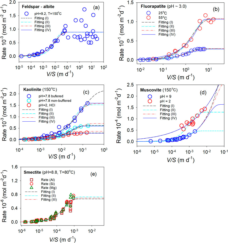
Figure 2. Dissolution rate as a function of V/S ratio. (a) Feldspar, (b) Fluorapatite, (c) Kaolinite, (d) Muscovite, and (e) Smectite. Symbols are experimental data. Lines are fitting results: dashed-lines (black, fitting (I) with m = 1), dashed-dot-lines (light blue, fitting (II) with m = 1 and q = 1, dashed-dot-dot-lines (red, fitting (III) with q = 1, solid-lines (blue, fitting (IV) without constraints.

For the datasets with sufficient data points at both low dissolution rates (near-equilibrium conditions) and near-plateau rates (i.e., maximum rates far from equilibrium) (Figures 2a–c), the fitted curves without constraints are, in most cases, indistinguishable from those fitted with various constraints. For feldspar (Figure 2a), the R² is approximately 0.68 for all constraints (I–IV). For fluorapatite (Figure 2b), the R² ranges from 0.97 to 0.99 at 25 °C and from 0.95 to 0.98 at 55 °C for all constraints. For kaolinite (Figure 2c), the R² ranges from 0.95 to 0.98 at buffered pH 7.8, is 0.99 at non-buffered pH 7.8, and ranges from 0.97 to 0.98 at pH 2.0, again for all constraint sets. In the case of buffered pH 7.8, due to the lack of data points at high V/S values, the projected rates at high V/S values vary, depending on the applied constraint (Figure 2c). These results suggest that fitting Equation 7 without constraints yields only marginal improvements in R² compared to fits using constrained models.

However, constraints are necessary for datasets lacking sufficient data points at low and/or high V/S values (Figures 2d,e) in order to achieve adequate fitting. For muscovite at pH = 2 (Figure 2d), the projected rates at high V/S values diverge under constraints I (m = 1.0), III (q = 1.0), and IV (no constraints), despite the fittings yielding R² values of 0.87–0.89. Under constraint II (q = 1.0 and m = 1.0), the projected rates converge around 1.3 × 10⁻⁴ mol m^-2 d^-1, although the R² drops to 0.61. Similar results were observed at pH = 9, except that without constraints (IV), the projected rates converge around 1.7 × 10⁻⁴ mol m^-2 d^-1, more than three times higher than the converged rate of 0.5 × 10⁻⁴ mol m^-2 d^-1 obtained under constraint II. For smectite (Figure 2e), the fittings under constraints I (m = 1.0), II (q = 1.0 and m = 1.0), and III (q = 1.0) are only slightly different, with R² values ranging from 0.94 to 0.95. However, without constraints (IV), the rate data could not be fitted due to large errors at high V/S values.

These fitting exercises suggest that, overall, Equation 7 can reasonably model the experimental dissolution data. The primary challenges in modeling arise from a lack of data points at far-from-equilibrium and/or near-equilibrium conditions, corresponding to high and low V/S values, respectively. For instance, any constraints applied to the fitting for feldspar (Figure 2a and fluorapatite (Figure 2b) would not make a significant difference from the fitting without constraints. Although constraining the exponent m or q to unity assumes, respectively, a defect-free material or a linear relationship between ${\Delta G}_r$ and V/S—both of which are incorrect—such constraints provide a baseline for interpreting the dissolution data and for guiding the design of future experiments.

3.2 Effect of $\mathit{m}$ and ${\chi }_{\mathit{d}}$ on dissolution rate

It would be interesting to see how m and ${\mathrm{\chi }}_d$ (q = 1) in Equation 7 affect the dissolution rate and results are shown in Figure 3a. For m = 1, an increase in ${\mathrm{\chi }}_d$ (dashed lines) shifts the curve to the right, resulting in larger V/S values at which the rate reaches its maximum (i.e., the plateau). Materials with higher V/S values at the dissolution rate maximum are those with higher ${\mathrm{\chi }}_d$ values and correspondingly higher dissolution rates (Figure 2). For instance, as shown in Figure 2b, a higher maximum dissolution rate (∼0.11 mol m^-2 d^-1 at 55 °C vs. ∼0.03 mol m^-2 d^-1 at 25 °C) corresponds to a higher V/S at the rate maximum (∼10 m d^-1 at 55 °C vs. 2 m d^-1 at 25 °C) and a higher ${\mathrm{\chi }}_d$ value (2.1 d m^-1 at 55 °C vs. 1.1 d m^-1 at 25 °C). Similar relationships are observed across different minerals (Figure 2). The maximum dissolution rates for fluorapatite (Figures 2b, 55 °C), feldspar and kaolinite (Figures 2a,c), muscovite (Figure 2d), and smectite (Figure 2e) are approximately in the order of 10^–1, 10^–3, 10^–4, and 10^–6 mol m^-2 d^-1, respectively. The corresponding V/S values are approximately in the order of 10¹, 10^–1, 10^–2, and 10^–3 m d^-1, and the ${\mathrm{\chi }}_d$ values follow a similar trend in the order of 10¹, 10^–1, 10^–2, and 10^–3 d m^-1, respectively. Therefore, ${\mathrm{\chi }}_d$ can serve as a descriptor of a material’s susceptibility to dissolution. Under a given set of conditions, the higher the ${\mathrm{\chi }}_d$ value of a material, the higher the dissolution rate it can attain.

Figure 3

Figure 3. Relative dissolution rate as a function of V/S ratio at a given condition. (a) The dashed lines are dissolution rates at $m=1.0$ and ${\chi }_d$ is in the range from 10, to 0.0001. The solid lines are the rates for ${\chi }_d=1.0$ and $m$ is in a range from 0.8 to 0.2. (b) Selected experiment release rates are plotted with the model at different ${\chi }_d$ values with m = 1 (dashed lines). The experimental data are from Figures 2b,c,e: fluorapatite (triangles, 2b (pH = 2 dark green; pH = 7.8 pink)), kaolinite (squares, 2c (55 °C red; 25 °C blue)) and smectite (cyan circles, 2e).

For a given ${\mathrm{\chi }}_d$ value (1.0), as shown in Figure 3a, a decrease in m from 0.8 to 0.2 (solid lines) does not affect the V/S value at which the dissolution rate reaches its maximum but increases the rate at a given V/S under low V/S conditions (i.e., near-equilibrium conditions). The higher rates at low V/S values can be attributed to surface defect–induced dissolution kinetics, such as those involving screw dislocations. This interpretation of m in Equation 7 is consistent with previous literature, which associates deviations from linear rate laws with the influence of crystal defects on dissolution reactions (Brantley, 2008; Schott et al., 2009; Lasaga, 1984).

To illustrate the relationship between the relative rate and V/S, the model is plotted along with selected dissolution data from the literature (Figure 3b). As shown, the trend of the experimental data follow the curves of the model with different ${\mathrm{\chi }}_d$ values, which indicate the magnitude of a material’s susceptibility to dissolution. As ${\mathrm{\chi }}_d$ becomes smaller (from the right to the left in Figure 3b), the dissolution rate decreases from fluorapatite, kaolinite, and to smectite at a given V/S, in the order of lower susceptibilities to dissolution.

3.3 Modeling of nuclear waste glass and ceramic forms

Equation 7 is derived from the dissolution data of well-studied minerals. Reasonable modeling results of applying the relationship are expected. It would be interesting to see how Equation 7 performs in modeling the dissolution rate data of less well-studied materials, for which complete thermodynamic data are often not available. Figure 4 shows dissolution rate data for a nuclear waste glass and a ceramic waste form (iodoapatite). For the apatite, the rates were reported in the elemental release in moles per day divided by the material’s surface area (moles/m²/d). For the nuclear glass, the rates are the elemental release in grams per day and divided by the surface area of the material (g/m²/d). Gibbs free energy of dissolution and solubility data are unavailable for these two datasets. For the nuclear glass (Figures 4a,b), the best fits were achieved with R² > 0.98, using Equation 7 with q = 1 and m = 1 constraints. For iodoapatite, the best fit was achieved using q = 1 and m = 1, with R² = ∼0.99. Fitting could not be completed without constraints, and the rate diverged at high V/S values. The requirement of constraints were resulted from a lack of experimental data points at low and high V/S values, especially the latter, which is a flaw in both of the experimental designs. The projected dissolution rate at far-from-equilibrium conditions is noticeably higher than the maximum observed rate in all three experiments. Additional experiments at higher V/S values are needed to fully understand their dissolution behavior. Due to the limited and suitable dissolution data available for nuclear waste materials, these two systems, however, provide a demonstration of the application of the relationship. In order to establish the general applicability of the relationship, more dissolution data for a wide range of materials are needed, especially those data at conditions in a full range of V/S ratio.

Figure 4

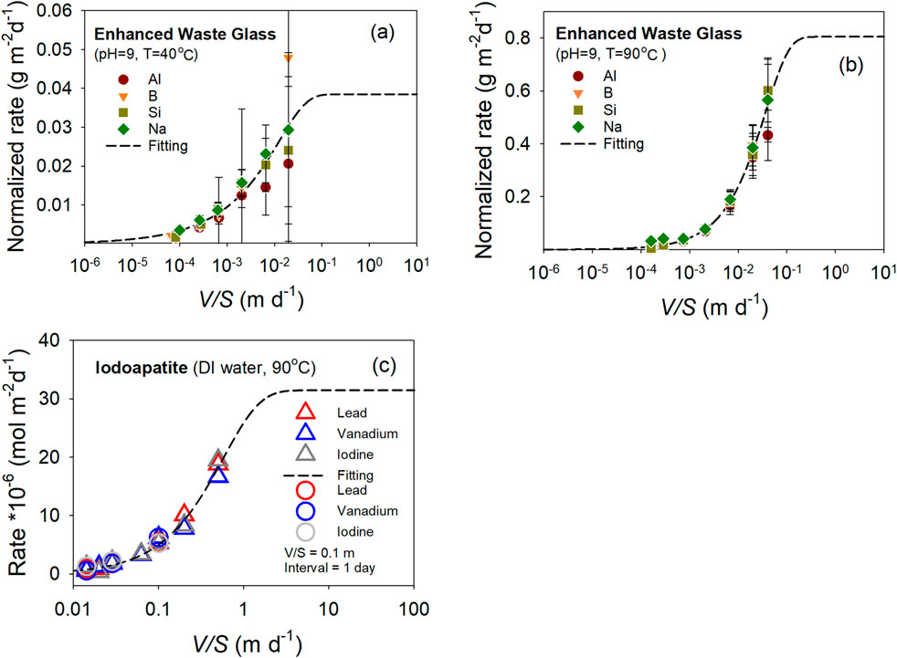
Figure 4. Dissolution rate as a function of V/S ratio for Enhanced Waste Glass at pH = 9 °C and 40 °C (a) and 90 °C (b), and iodoapatite with DI water at 90 °C (c). A Cauchy weighting function was used to account for an increase of errors as $V/S$ increases. The dashed lines are fitting results.

The results from both Figures 2, 4 suggest that dissolution rate data with sufficient points at far-from-equilibrium and close-to-equilibrium conditions are well described by Equation 7. Even with fewer data points, Equation 7 can be used to model the dissolution data and provide feedback for improving the experimental design in future investigations, suggesting the robustness of Equation 7 in describing dissolution kinetics. It needs to be clarified that the modeling is numerical in natural and can only provide guidance on the dissolution state by V/S ratio. They do not inform dissolution mechanisms in these materials. In case of glass, its dissolution is complex and multi-staged.

3.4 Effect of solution composition on dissolution rate

Sections 3.1 and 3.3 describe the dissolution kinetics at constant solution composition. If the solution composition in dissolution experiments varies, the rate changes. The effects of solution composition on dissolution rate are well documented in the literature (Devidal et al., 1997; Schott et al., 2009). By combining the composition effect on dissolution rate with Equation 7, the following equation can be used to model the rate data of these oxides measured under varying solution compositions.

$r=k_{+}\left[\frac{K_p^{*}{\left[\frac{a_{H^{+}}^z}{a_{M^{+}}}\right]}^n}{1+K_p^{*}{\left[\frac{a_{H^{+}}^z}{a_{M^{+}}}\right]}^n}\right]{\left(1-e^{-{\left(V/S\right)}^q/{\mathrm{\chi }}_d}\right)}^m(8)$

Where $k_{+}$ is the rate constant, $K_p^{*}$ the equilibrium constant for precursor formation, z the charge on the aqueous cation M, and n the number of cations that must be removed to create the surface precursor. $a_{H^{+}}$ is the activity of H⁺, and $a_{M^{+}}$ the activity of M⁺. The second term describes the effect of the composition on the forward rate at a given set of conditions.

The experimental data at a given pH and temperature, with varying solution compositions for kaolinite, are plotted in Figures 5a,b (Devidal et al., 1997), clearly showing the effect of solution composition on the dissolution rate. To model the rate using Equation 7, the original rates were normalized by applying the second term of Equation 8 and are plotted in Figure 5c for the data at pH = 2, and in Figure 5d for the data at pH = 7.8. For kaolinite, M = Al³⁺, z = 3, and n = 1 (Devidal et al., 1997). These normalized rates were then modeled using Equation 7, with the constraints m = 1 and q = 1 applied during fitting due to a lack of data at high V/S values. All the rate data from different solution compositions were included in the fitting. The dashed lines represent fitted curves (Figures 5c,d), with R² = 0.93 for the data at pH = 2 and R² = 0.96 for the data at pH = 7.8. Given the uncertainties in the data, the fits are reasonably acceptable. These results suggest that the proposed relationship in Equation 7 can be extended by incorporating terms representing other environmental variables, in this case, solution composition.

Figure 5

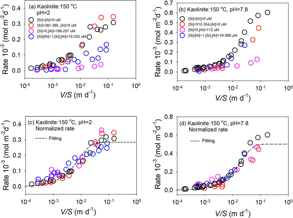
Figure 5. The dissolution rate of kaolinite at 150 °C as a function of solution V/S and solution composition at pH = 2 (a) and pH = 7.8 (b). The normalized rates are plotted as a function of V/S for pH = 2 (c) and pH = 7.8 (d). The dashed lines are fitting results.

4 Summary and concluding remarks

Dissolution kinetics is fundamentally important to materials science, as the chemical durability of materials is critical to the safety, cost, and efficiency of their applications. Modeling the dissolution rate under various environmental conditions is essential for understanding dissolution behavior and guiding experimental design. Due to the lack of thermodynamic data—such as the Gibbs free energy of dissolution—for complex nuclear waste materials like nuclear glass, rate equations based on activity products or saturation indices cannot be applied to model nuclear waste glass dissolution kinetics. Instead, the ratio of the reacting solution volume to the surface area of the dissolving material per unit time (V/S ratio) is employed as an environmental variable. An empirical relationship between the Gibbs free energy and the V/S ratio was proposed, allowing the dissolution rate to be related to V/S. This empirical relation was subsequently applied to model the dissolution of several minerals, a ceramic waste form, and a nuclear glass. Such modeling enables monitoring of dissolution experiments, provides feedback for experimental design, and offers insights into dissolution kinetics.

Dissolution is a complex phenomenon, and its kinetics cannot be accurately described using a single parameter. The dissolution rate is not an intrinsic property of a material but rather a response to environmental variables. This presents a challenge in characterizing the chemical durability of nuclear waste materials. Therefore, it is essential to evaluate properties that can distinguish materials with different intrinsic chemical durability. Although standard test protocols have been developed to assess the chemical durability of nuclear waste materials, the rate itself cannot serve this purpose, as it is not an intrinsic property. This study demonstrates that the dissolution susceptibility of a material, denoted as ${\mathrm{\chi }}_d$, can be used as a parameter to distinguish the chemical durability of different materials.

Data availability statement

The original contributions presented in the study are included in the article/supplementary material, further inquiries can be directed to the corresponding author.

Author contributions

JW: Conceptualization, Data curation, Formal Analysis, Funding acquisition, Investigation, Methodology, Project administration, Resources, Validation, Visualization, Writing – original draft, Writing – review and editing.

Funding

The author(s) declare that financial support was received for the research and/or publication of this article. This work was supported as part of the Center for Performance and Design of Nuclear Waste Forms and Containers, an Energy Frontier Research Center funded by the U.S. Department of Energy, Office of Science, Basic Energy Sciences, under Award DE-SC0016584.

Acknowledgements

JW is grateful for the support from the Charles L. Jones Endowed Professorship in Geology and Geophysics at Louisiana State University.

Conflict of interest

The author declares that the research was conducted in the absence of any commercial or financial relationships that could be construed as a potential conflict of interest.

The author(s) declared that they were an editorial board member of Frontiers, at the time of submission. This had no impact on the peer review process and the final decision.

Generative AI statement

The author(s) declare that no Generative AI was used in the creation of this manuscript.

Any alternative text (alt text) provided alongside figures in this article has been generated by Frontiers with the support of artificial intelligence and reasonable efforts have been made to ensure accuracy, including review by the authors wherever possible. If you identify any issues, please contact us.

Publisher’s note

All claims expressed in this article are solely those of the authors and do not necessarily represent those of their affiliated organizations, or those of the publisher, the editors and the reviewers. Any product that may be evaluated in this article, or claim that may be made by its manufacturer, is not guaranteed or endorsed by the publisher.

References

Aagaard, P., and Helgeson, H. C. (1982). Thermodynamic and kinetic constraints on reaction-rates among minerals and aqueous-solutions (I) theoretical considerations. Am. J. Sci. 282 (3), 237–285. doi:10.2475/ajs.282.3.237

CrossRef Full Text | Google Scholar

ASTM-C1285-14 (2014). Standard test methods for determining chemical durability of nuclear, hazardous, and mixed waste glasses and multiphase glass ceramics: the product consistency test. PCT. doi:10.1520/C1285-21

CrossRef Full Text | Google Scholar

ASTM-C1308-08 (2009). Accelerated leach test for diffusive releases from solidified waste and a computer program to model diffusive, fractional leaching from cylindrical waste forms. West Conshohocken, PA: ASTM International. doi:10.1520/C1308-08R17

CrossRef Full Text | Google Scholar

ASTM-C1662-18 (2018). Standard practice for measurement of the glass dissolution rate using the single-pass flow-through test method. West Conshohocken, PA: ASTM International.

Google Scholar

Brantley, S. L. (2008). “Kinetics of mineral dissolution,” in Kinetics of water-rock interaction (Springer), 151–210.

Google Scholar

C1220-21, A. (2010). Standard test method for static leaching of monolithic waste forms for disposal of radioactive waste.

Google Scholar

Cama, J., Ganor, J., Ayora, C., and Lasaga, C. A. (2000). Smectite dissolution kinetics at 80 C and pH 8.8. Geochimica Cosmochimica Acta 64 (15), 2701–2717. doi:10.1016/S0016-7037(00)00378-1

CrossRef Full Text | Google Scholar

Devidal, J.-L., Schott, J., and Dandurand, J.-L. (1997). An experimental study of kaolinite dissolution and precipitation kinetics as a function of chemical affinity and solution composition at 150 C, 40 bars, and pH 2, 6.8, and 7.8. Geochimica Cosmochimica Acta 61 (24), 5165–5186. doi:10.1016/S0016-7037(97)00352-9

CrossRef Full Text | Google Scholar

Frankel, G. S., Vienna, J. D., Lian, J., Scully, J. R., Gin, S., Ryan, J. V., et al. (2018). A comparative review of the aqueous corrosion of glasses, crystalline ceramics, and metals. npj Mater. Degrad. 2 (1), 15. doi:10.1038/s41529-018-0037-2

CrossRef Full Text | Google Scholar

Frankel, G. S., Vienna, J. D., Lian, J., Guo, X., Gin, S., Kim, S. H., et al. (2021). Recent advances in corrosion science applicable to disposal of high-level nuclear waste. Chem. Rev. 121 (20), 12327–12383. doi:10.1021/acs.chemrev.0c00990

PubMed Abstract | CrossRef Full Text | Google Scholar

Frankel, G. S., Du, J., Gin, S., Kim, S. H., Lian, J., Locke, J. W., et al. (2023). The center for performance and design of nuclear waste forms and containers (WastePD) energy frontier research center. doi:10.2172/1905097

CrossRef Full Text | Google Scholar

Guidry, M. W., and Mackenzie, F. T. (2003). Experimental study of igneous and sedimentary apatite dissolution: control of pH, distance from equilibrium, and temperature on dissolution rates. Geochimica Cosmochimica Acta 67 (16), 2949–2963. doi:10.1016/S0016-7037(03)00265-5

CrossRef Full Text | Google Scholar

Hellmann, R., and Tisserand, D. (2006). Dissolution kinetics as a function of the gibbs free energy of reaction: an experimental study based on albite feldspar. Geochimica Cosmochimica Acta 70 (2), 364–383. doi:10.1016/j.gca.2005.10.007

CrossRef Full Text | Google Scholar

Kotowski, M., and van Eldik, R. (1989). Application of high pressure kinetic techniques to mechanistic studies in coordination chemistry. Coord. Chem. Rev. 93 (1), 19–57. doi:10.1016/0010-8545(89)80011-6

CrossRef Full Text | Google Scholar

Lasaga, A. C. (1984). Chemical kinetics of water-rock interactions. J. Geophys. Res. solid earth 89 (B6), 4009–4025. doi:10.1029/JB089iB06p04009

CrossRef Full Text | Google Scholar

Lasaga, A. C., Soler, J. M., Ganor, J., Burch, T. E., and Nagy, K. L. (1994). Chemical weathering rate laws and global geochemical cycles. Geochimica Cosmochimica Acta 58 (10), 2361–2386. doi:10.1016/0016-7037(94)90016-7

CrossRef Full Text | Google Scholar

Nabyl, Z., Schuller, S., Podor, R., Lautru, J., Sauvage, E., Artico, A., et al. (2024). French nuclear glass synthesis: focus on liquid waste dissolution kinetics. J. Nucl. Mater. 601, 155329. doi:10.1016/j.jnucmat.2024.155329

CrossRef Full Text | Google Scholar

Nagy, K. L., and Lasaga, A. C. (1992). Dissolution and precipitation kinetics of gibbsite at 80 °C and pH 3: the dependence on solution saturation state. Geochimica Cosmochimica Acta 56 (8), 3093–3111. doi:10.1016/0016-7037(92)90291-P

CrossRef Full Text | Google Scholar

National Research Council (1999). Disposition of high-level radioactive waste through geological isolation: development, current status, and technical and policy challenges. Washington, DC: National Academies Press. doi:10.17226/9674

CrossRef Full Text | Google Scholar

Oelkers, E. H., Schott, J., Gauthier, J.-M., and Herrero-Roncal, T. (2008). An experimental study of the dissolution mechanism and rates of muscovite. Geochimica Cosmochimica Acta 72 (20), 4948–4961. doi:10.1016/j.gca.2008.01.040

CrossRef Full Text | Google Scholar

Schott, J., Pokrovsky, O. S., and Oelkers, E. H. (2009). The link between mineral dissolution/precipitation kinetics and solution chemistry. Rev. mineralogy Geochem. 70 (1), 207–258. doi:10.2138/rmg.2009.70.6

CrossRef Full Text | Google Scholar

Sherman, D. M. (2009). Surface complexation modeling: mineral fluid equilbria at the molecular scale. Rev. Mineralogy Geochem. 70 (1), 181–205. doi:10.2138/rmg.2009.70.5

CrossRef Full Text | Google Scholar

Sposito, G. (1983). On the surface complexation model of the oxide-aqueous solution interface. J. Colloid Interface Sci. 91 (2), 329–340. doi:10.1016/0021-9797(83)90345-4

CrossRef Full Text | Google Scholar

Strachan, D., Turcotte, R., and Barnes, B. (1982). MCC-1: a standard leach test for nuclear waste forms. Nucl. Technol. 56 (2), 306–312. doi:10.13182/NT82-A32859

CrossRef Full Text | Google Scholar

Stumm, W., and Wollast, R. (1990). Coordination chemistry of weathering: kinetics of the surface-controlled dissolution of oxide minerals. Rev. Geophys. 28 (1), 53–69. doi:10.1029/RG028i001p00053

CrossRef Full Text | Google Scholar

Truhlar, D. G., Garrett, B. C., and Klippenstein, S. J. (1996). Current status of transition-state theory. J. Phys. Chem. 100 (31), 12771–12800. doi:10.1021/jp953748q

CrossRef Full Text | Google Scholar

U.S. Department of Energy (2008). Yucca Mountain repository license application: safety analysis report. Washington, DC: U.S. Nuclear Regulatory Commission.

Google Scholar

Wang, J. (2020). Thermodynamic equilibrium and kinetic fundamentals of oxide dissolution in aqueous solution. J. Mater. Res. 35 (8), 898–921. doi:10.1557/jmr.2020.81

CrossRef Full Text | Google Scholar

Zhang, Z., Ebert, W. L., Yao, T., Lian, J., Valsaraj, K. T., and Wang, J. (2019). Chemical durability and dissolution kinetics of iodoapatite in aqueous solutions. ACS Earth Space Chem. 3 (3), 452–462. doi:10.1021/acsearthspacechem.8b00162

CrossRef Full Text | Google Scholar