Ensembles of physics-enhanced neural networks for the prediction of critical heat flux in nuclear reactors and the quantification of its uncertainty

The Critical Heat Flux (CHF) is a physical phenomenon that may cause the deterioration of the heat transfer in the core of nuclear reactors, potentially leading to core damage. Its accurate prediction is therefore a crucial issue in nuclear reactor safety. To this aim, various empirical and mechanistic models have been proposed to estimate the CHF across various flow regimes and conditions, which however present some drawbacks: i) data scarcity in some parts of the input domain; ii) no information about prediction uncertainties; iii) difficult explainability and interpretability of the results. To address these issues, ensembles of Physics-Enhanced Neural Networks (PENNs) are considered to predict the CHF as a function of relevant physical input variables (e.g., pipe heated length and diameter, pressure, mass flux, outlet quality). Two different frameworks to integrate physics and data-driven NN-based strategies are here compared for the first time, to the best of the author’s knowledge. In the first, fixed-structure (prior) baseline models (i.e., the Groeneveld Look-Up Table-LUT and the mechanistic Liu model) are constructed relying on the existing knowledge on the physical phenomenon of interest, which serves as a reference solution; then, NN ensembles are employed to capture unknown, unexplored information from the mismatch (i.e., the residuals) between the real CHF values and the estimates produced by the knowledge-based models. In the second, the LUT and the mechanistic Liu model are directly implemented in the NN loss function for effective (physics- and data-driven) ensemble training. A case study is carried out with an extensive CHF database (published by the U.S. Nuclear Regulatory Commission with measurements in vertical uniformly-heated water-cooled cylindrical tubes) to demonstrate: i) the improved performance of the PENN-based approaches as compared to traditional knowledge-based models; ii) the PENN superior generalization capabilities over standalone data-driven NNs in the presence of small-sized datasets (i.e., a few tens or hundreds points); iii) the possibility to build robustness in the CHF predictions by bootstrap and PENN weights random reinitialization for quantifying uncertainty and estimating prediction intervals.

1 Introduction

Critical Heat Flux (CHF) is a fundamental parameter in the thermal-hydraulic design and safe operation of heat-generating systems, particularly nuclear reactors. CHF denotes the thermal limit at which the heat transfer from a heated surface to the coolant deteriorates drastically as the surface heat flux increases. Beyond this threshold, the cooling mechanism becomes insufficient, resulting in a sharp rise in surface temperature. Exceeding CHF conditions necessitates immediate shutdown procedures to prevent damage to the system and mitigate production losses. In severe cases, surpassing CHF can lead to significant structural failures, including fuel cladding rupture and potential core degradation in nuclear applications (Todreas and Kazimi, 2021; Khalid et al., 2024a). Two distinct mechanisms are primarily responsible for the onset of CHF: Departure from Nucleate Boiling (DNB) and dryout (DO). DNB typically occurs under low-quality flow conditions, where the coolant is predominantly in the liquid phase. In such cases, localized vapor production can form an insulating vapor blanket over the heated surface, suppressing nucleate boiling and leading to a rapid increase in surface temperature. In contrast, DO is characteristic of high-quality flow regimes, where a vapor core containing entrained droplets is surrounded by a thin liquid film along the channel walls. CHF due to DO occurs when this annular liquid film is depleted, eliminating the primary cooling mechanism at the surface. While both mechanisms are of concern in various heat transfer systems, their implications in nuclear reactors are particularly critical. DNB and DO can result in heat transfer deterioration severe enough to cause fuel cladding failure, and in extreme scenarios, lead to fuel melting. In conventional systems such as boilers and heat exchangers, DO may result in reduced thermal efficiency or mechanical failure, such as tube rupture. Given these risks, CHF is recognized as a key safety-related quantity in nuclear engineering. Its accurate prediction is essential during the thermal-hydraulic analysis and design phases to ensure operating conditions remain within safe margins. Predictive models and experimental validation are thus vital for maintaining system integrity and operational reliability (Zhao et al., 2020; 2021; Furlong et al., 2025a).

Extensive research has been devoted to understanding and predicting Critical Heat Flux (CHF), with the primary objective of developing a unified model capable of reliably forecasting its occurrence across a broad range of operating conditions and geometries. However, this endeavor remains challenging due to the strong dependence of CHF on reactor configuration, operational parameters, fuel rod geometry, and coolant thermophysical properties. Compounding this complexity is the lack of consensus on the fundamental mechanisms responsible for CHF onset. The precise triggering phenomena are still the subject of ongoing debate, largely due to the inherently complex nature of boiling heat transfer and phase-change dynamics (Celata et al., 1994; Bucci, 2017). As a result, the thermal engineering community has proposed a wide array of predictive approaches - numbering over 500 - that attempt to address various aspects of CHF behavior. These models can be broadly categorized into three principal frameworks (Kandlikar, 2001; Bruder et al., 2017; Groeneveld et al., 2018; Yang B.-W. et al., 2021): (i) empirical correlations developed through experimental data fitting (e.g., Hall and Mudawar, 2000; Todreas and Kazimi, 2021); (ii) Look-Up Tables (LUTs) derived from extensive experimental databases (Groeneveld et al., 2007; Groeneveld, 2019); and (iii) physics-based mechanistic models that attempt to resolve the underlying physical processes driving CHF (Okawa et al., 2004; Liu, 2022). Empirical correlations constitute a statistical modeling approach used to predict CHF based on observed relationships among experimentally measured variables. These correlations typically take the form of polynomial or other analytical expressions, enabling CHF estimation under conditions similar to those for which the underlying data were obtained. While widely employed due to their simplicity and computational efficiency, empirical correlations are inherently limited in their generalizability. Since they are derived from specific datasets, their predictive accuracy often deteriorates when applied outside the original experimental conditions or under differing boundary parameters. For instance, a correlation developed for a particular coolant, geometry, or pressure range may yield unreliable predictions when extrapolated to other configurations. The reliability of these models is also contingent upon the quality, representativeness, and scope of the experimental data used in their formulation. Consequently, empirical correlations must be applied with caution and rigorously validated against relevant experimental datasets prior to deployment in safety-critical applications. Several widely used empirical CHF models have been developed over the decades, each typically associated with either DNB or DO mechanisms. Notable examples include the Biasi (DNB) (Biasi et al., 1967), the Bowring (DO) (Bowring, 1972), the Westinghouse W-3 (DNB) (Tong, 1967), the Katto (DNB) (Katto, 1978; 1992), and the Electric Power Research Institute (EPRI) correlations (Reddy and Fighetti, 1983). The second major approach for predicting CHF is the use of Look-Up Tables (LUTs), which offer a systematic and relatively precise method for estimation. Unlike empirical correlations, LUTs are constructed from extensive experimental datasets, enabling interpolation across a wide range of operational parameters. However, the development of accurate LUTs necessitates considerable preparatory work, including the acquisition and rigorous analysis of large volumes of high-quality experimental data. A prominent example is the Groeneveld LUT (Groeneveld et al., 2007; Groeneveld, 2019), which was developed by aggregating data from 59 separate experiments. This comprehensive dataset contains nearly 25,000 entries, representing CHF measurements for uniformly heated vertical tubes under both DNB and DO conditions, and is parameterized by seven key input variables. In contrast, physics-based mechanistic models aim to predict CHF by incorporating assumptions grounded in the physical understanding of underlying flow boiling phenomena. These models typically solve conservation equations that are closed using empirically derived constitutive relationships (Zhao et al., 2020). While mechanistic models have the potential to provide greater insight into the governing processes, their development and application are inherently complex and demand a high degree of expertise. This is due, in part, to the dependence of CHF mechanisms on flow regime, channel geometry, and boundary conditions (Yan et al., 2021; Khalid et al., 2024a). A wide range of mechanistic models for flow boiling has been proposed in the literature. These can be broadly classified into six categories based on the hypothesized dominant DNB mechanism (Zhao et al., 2020): (i) liquid layer superheat limit, (ii) boundary layer separation, (iii) liquid flow blockage, (iv) near-wall bubble crowding, (v) liquid sublayer DO, and (vi) interfacial lift-off (Bruder et al., 2017). Among these, the liquid sublayer DO mechanism has received significant attention, supported by experimental evidence in internally heated round tubes (Katto, 1990). Notable sublayer DO-based models include those developed by Lee and Mudawwar (1988), Katto (1990), Celata et al. (1994), (1999), Liu et al. (2000), and Liu (2022). Despite the capabilities of empirical correlations, LUTs, and mechanistic models in predicting CHF across a broad range of input conditions, significant deviations from experimental measurements persist in various regions of the operational space (Groeneveld et al., 2007). These limitations have continued to motivate ongoing research efforts aimed at developing more accurate and robust predictive methodologies.

Recent advancements in computational power and optimization algorithms have enabled the emergence of purely data-driven approaches based on Machine Learning (ML) and Artificial Intelligence (AI) as viable alternatives to conventional CHF prediction methods (Huang et al., 2023). These include, among the others: Deep Neural Networks (DNNs), deep AutoEncoders (AEs), Deep Belief Networks (DBNs), Convolutional Neural Networks (CNNs), Conditional Variational Autoencoders (CVAEs), Support Vector Machines (SVMs), Random Forests (RFs), and Gaussian Process Regression (GPR) (Alsafadi et al., 2025; Grosfilley et al., 2024; Khalid et al., 2024a; Kim et al., 2021; Kumar et al., 2024; Zhao et al., 2020; Zhou et al., 2024). Such techniques operate by learning patterns from training data without requiring explicit knowledge of the underlying physical processes. One of the principal advantages of ML- and AI-based models lies in their capacity to uncover complex, non-linear relationships within high-dimensional datasets - relationships that may be difficult or impossible to identify using traditional empirical or mechanistic methods. This capability often translates into improved predictive accuracy across diverse operating conditions. Additionally, once trained, these models are computationally efficient and inexpensive to deploy, further enhancing their practical appeal. The growing body of literature in this domain underscores the increasing interest and success of data-driven approaches in thermal-hydraulic applications (Qi et al., 2025).

Although standalone AI and ML methods offer the advantage of requiring minimal prior knowledge and no explicit mathematical modeling, their practical deployment is hindered by several notable limitations (Cicirello, 2024; Lye et al., 2025). Key challenges include: (1) poor data quality; (2) limited availability of reliable training data; (3) weak extrapolation and generalization capabilities under previously unseen conditions; (4) the presence of significant uncertainties; and (5) limited interpretability of the resulting models. A particularly critical concern is their susceptibility to generating unphysical or non-intuitive outputs, stemming from their purely data-driven and often “black-box” nature. As model complexity grows - often involving thousands to millions of tunable parameters depending on the algorithm and application - the potential for overfitting, instability, and loss of transparency increases. This poses a substantial barrier for high-stakes applications such as nuclear thermal-hydraulics, where model reliability, traceability, and interpretability are essential for ensuring safety and regulatory compliance. Data scarcity and poor data quality further exacerbate these challenges. For example, in some engineering problems and applications, traditional AI/ML architectures, such as DNNs, may require large volumes of high-quality data to attain satisfactory predictive performance (Hong et al., 2023; Shi and Zhang, 2022; Zhao et al., 2022; Zhu et al., 2022). Inadequate data, or datasets contaminated with noise, can significantly impair model training, leading to degraded performance or complete model failure. Although various data augmentation strategies have been proposed to alleviate the issue of limited data (Kim et al., 2021; Zhang et al., 2022; Alsafadi et al., 2025), such approaches still fall short in guaranteeing physically consistent outputs or providing interpretability, both of which are essential for deployment in critical engineering domains.

To address the limitations associated with purely data-driven models, recent research has focused on integrating domain-specific physical knowledge into the AI/ML framework, leading to the development of Physics-Enhanced Machine Learning (PEML) approaches¹ (Furlong et al., 2025a; Mao and Jin, 2024; Zhao et al., 2020). These hybrid methodologies aim to combine the predictive power of data-driven techniques with the rigor and consistency of established physical laws governing nuclear systems. By embedding physical constraints and principles directly into the ML training process, PEML frameworks ensure that the learned models produce outputs that are not only data-consistent but also physically plausible and aligned with underlying conservation laws and mechanistic correlations. The fusion of reliable physical laws and data is expected to allow the model to generalize more effectively, to improve predictive accuracy, and to possibly enhance interpretability - key requirements for deployment in safety-critical fields such as nuclear engineering. Rather than relying solely on statistical patterns in the data, the learning algorithm is guided by physically informed structures or loss functions, enabling it to learn complex relationships while adhering to known physical behavior (Cicirello, 2024; Lye et al., 2025).

Given the complexity and non-linearity of the relationships between the physical input parameters and the CHF, in this paper Neural Networks (NNs) are selected as AI/ML techniques for their capability to capture intricate patterns and dependencies within the data (Zhao et al., 2020; Grosfilley et al., 2024). Then, the main objective is to systematically compare two different approaches to integrate physics and data-driven NN strategies, within a Physics-Enhanced Neural Network (PENN) framework:

1. The empirical Groeneveld LUT (Groeneveld et al., 2007; Groeneveld, 2019) and the mechanistic Liu model (Liu et al., 2000; 2012; Liu, 2022) are taken as (prior) reference, fixed-structure baseline solutions, since they rely on the existing knowledge on the physical phenomena of interest. Then, NNs are employed to capture unknown, unexplored information from the mismatch (i.e., the residuals) between the real CHF values and the estimates produced by the knowledge-based models, as proposed in Zhao et al. (2020). Notice that different from Zhao et al. (2020), the improved mechanistic physics-based model presented in Liu et al. (2012) is here adopted instead of that included in Liu et al. (2000). Hereafter, this approach will be referred to as Residual-based Physics-Enhanced Neural Network (Res-PENN).

2. The two reference models mentioned above (i.e., LUT and Liu) are implemented directly in the NN loss function for effective (hybrid physics- and data-driven) training. In other words, the PENN training is guided by two terms: i) the discrepancy between the NN prediction and the experimental data; ii) the difference between the NN estimates and the prior, baseline physics-based model outputs. Hereafter, this approach will be referred to as Hybrid Loss Function-based Physics-Enhanced Neural Network (HLF-PENN).

While the HLF-PENN methodology has proven beneficial across a variety of physics domains (Cuomo et al., 2022; De La Mata et al., 2023; Cicirello, 2024), including but not limited to fluid dynamics (Jin et al., 2021), structural mechanics (Diao et al., 2023; Marino and Cicirello, 2023; Yang et al., 2025), and heat transfer (Karpatne et al., 2017; Cai et al., 2021; Jalili et al., 2024), to the best of the author’s knowledge, few or no applications to CHF prediction in nuclear reactors are available in the open literature (Ahmed et al., 2025). Also, it is the first time that the Res-PENN and HLF-PENN approaches are systematically compared, with particular reference to the task of estimating CHF in the presence of very scarce data (i.e., a few tens or hundreds training patterns). This aspect is of paramount importance in the nuclear industry, where collecting a large amount of high-quality data is often too costly (and sometimes even impossible).

Finally, the uncertainty in CHF predictions of the two configurations above is quantified by an ensemble-based approach, conceived as an original combination of two nested procedures. On the one hand, we resort to the bootstrap method, i.e., a non-parametric statistical approach, in which many different NN models are trained each time using a different set of data, obtained by random sampling with replacement of the original training set. The resulting ensemble of NN models is then exploited to construct an empirical probability distribution of output responses (CHF predictions). This distribution reflects the portion of NN uncertainty due to the presence of a finite-sized (thus limited and incomplete) training dataset (Efron and Tibshirani, 1994; Abrate et al., 2023a; b). On the other hand, we adopt an initialization-based strategy, where different randomized weight/bias starting values are used to train a set of NN models, each of which subsequently explores a different solution space to attempt to find a global minimum of the objective function (LeCun et al., 2015; Furlong et al., 2025a). This approach allows us to assess the portion of uncertainty resulting from other sources than finiteness of the training dataset, such as randomness in the training process, model architecture, etc. (Yaseen and Wu, 2023; Tan et al., 2023).

The proposed methods are compared using the United States Nuclear Regulatory Commission (USNRC) CHF dataset from (Groeneveld, 2019) made available by the Working Party on Scientific Issues and Uncertainty Analysis of Reactor Systems (WPRS) Expert Group on Reactor Systems Multi-Physics (EGMUP) task force on AI and ML for Scientific Computing in Nuclear Engineering projects, promoted by the OECD/NEA (Le Corre et al., 2024).

The remainder of the paper is organized as follows. In Section 2, a detailed literature review on AI and ML methods for CHF estimation is provided. In Section 3, the CHF prediction problem is rigorously stated, while the PENN-based ensembles selected to address it are presented in detail in Section 4. The case study is described in Section 5, while the corresponding results obtained by the PENNs are thoroughly discussed in Section 6. Finally, some conclusions are drawn in Section 7.

2 Artificial intelligence (AI) and machine learning (ML) for critical heat flux (CHF) prediction: a detailed literature review

With recent advances in computational capabilities and optimization techniques, methods based on purely data-driven Machine Learning (ML) and Artificial Intelligence (AI) provide an alternative approach to existing tools (Huang et al., 2023). These approaches rely on fitting parameters to training data and do not require any knowledge about the physical world or problem. The primary benefits of these approaches are their ability to find relationships that may not be readily apparent in the data (often leading to higher overall accuracy in comparison with traditional methods) as well as their inexpensive nature and quick performance post-training. This is demonstrated by the flourishing literature in the field (Qi et al., 2025). With reference only to the last 5–10 years (He and Lee, 2018), employ Support Vector Machines (SVMs) for data-driven CHF look-up table construction based on sparingly distributed training data points, showing appreciable performance also in extrapolation tasks. The same authors compare various machine learning methods, including ν-SVM, Back-Propagation Neural Network (BPNN), Radial Basis Function (RBF), General Regression Neural Network (GRNN), and Deep Belief Network (DBN) in the task of estimating CHF on microstructure surface by means of data from horizontal silicon specimens of cylindrical pillars with square arrangements (He and Lee, 2020). In (Park et al., 2020), Artificial Neural Networks (ANNs) are used to predict the wall temperature from a nucleate boiling heat transfer model at a given CHF within the thermal-hydraulic system code SPACE. ANNs are adopted also by Mudawar et al. (2024) for predicting flow boiling heat transfer and critical heat flux in both microgravity and Earth gravity for space applications. In (Jiang et al., 2020), a hybrid approach based on Gaussian Process Regression (GPR) and Ant Colony Optimization (ACO) is proposed for the prediction of CHF: in this model, the ACO algorithm is employed to optimize the hyper-parameters of GPR based on a training set derived from two published literature sources (Hedayat, 2021). develops cascade feed-forward Artificial Neural Networks (ANNs) with Deep Learning (DL) features to predict a full range CHF in different LWRs via parallel multi-processing to reduce the computational cost. In (Kim et al., 2021) a Deep Belief Network (DBN) and a Residual Network (ResNet) are combined to predict CHF in narrow rectangular channels in a steady state condition. DBN is used to perform feature extraction in an unsupervised pre-training phase, whereas ResNet is employed for (supervised) CHF prediction, as it improves accuracy through residual learning. The combined neural network is trained by means of an augmented “pseudo-dataset”, synthetically generated using four existing CHF correlations to cover a wide range of conditions involving thermal-hydraulic, geometric, and heater parameters. In (Rassoulinejad-Mousavi et al., 2021) Convolutional Neural Networks (CNNs) and Transfer Learning (TL) are compared in the task of detecting CHF in pool boiling, with the main objective of progressively adapting the trained models to new datasets collected under different conditions. In (Swartz et al., 2021) the effectiveness of three ML models (i.e., Least Absolute Shrinkage and Selection Operator-LASSO, Deep Feedforward Neural Networks-DFNN, and Random Forest-RF) is assessed in the predictions of critical heat fluxes for pillar-modified surfaces. In (Rohatgi et al., 2022), the authors use a data augmentation methodology based on Generative Adversarial Networks (GANs) to expand the training set for an ANN to predict the power at which DNB occurs in Pressurized Water Reactors (PWRs) as a function of the outlet pressure, inlet temperature and inlet mass flux as the input features, within the PWR subchannel and bundle tests (PSBT) benchmark. An approach based on data augmentation is presented also by Alsafadi et al. (2025), where a Conditional Variational AutoEncoder (CVAE) is employed to produce specific input data instances (e.g., data samples at conditions and domains desired by the user) starting from an important set of CHF experimental data. The CVAE performance is satisfactorily compared to that of Deep Neural Networks (DNNs) also in the uncertainty quantification task, obtained by (CVAE) repeated sampling and (DNN) ensembles. The use of DNNs is explored also by Khalid et al. (2024a), where an ensemble of deep sparse AutoEncoders (AEs) is used as a base-learner to extract robust features from the experimental data and a DNN is built on top of the ensemble of deep sparse AEs as a meta-learner to predict the CHF based on six input parameters (Zhang et al., 2022). compare three machine learning methods, the ε-Support Vector Machine (ε-SVM), Back Propagation Neural Network (BPNN) and Random Forest (RF), in the prediction of CHF on downward facing surfaces, also with the aid of synthetic pseudo-data generated by a simple fitting process. Several other papers are devoted to the comparison of purely data-driven AI/ML techniques on CHF predictions (Kim et al., 2022a; Khalid et al., 2023; Li et al., 2024; Kumar et al., 2024). Take into account ANNs, RFs, SVMs and LUT. In (Grosfilley et al., 2024) ν-SVMs, GPR, and ANNs are applied to the 2006 Groeneveld CHF database (nearly 25,000 data points). The same database is used by Zhou et al. (2024) to carry out an assessment of some state-of-the-art AI methods for critical heat flux prediction (i.e., ANNs, CNNs, Transformers with self-attention mechanism and Transfer Learning-TL) (Cabarcos et al., 2024). use a geometrical model of a rectangular channel at an inclined angle to evaluate the predictive performance of five ML models using collected CHF data: ANNs, AdaBoost, RF, XGBoost, and SVM. Most of these techniques (with the addition of K-Nearest Neighbors-KNN) are also embraced by Khalid et al. (2024b) to study the dependence of CHF in vertical flow systems on dimensional and dimensionless parameters. Finally (Quadros et al., 2024), analyze bubble departure and lift-off boiling model by computational intelligence techniques and hybrid algorithms, such as ANNs, the Fuzzy Mamdani model, Adaptive Neuro-Fuzzy Inference System (ANFIS) and ANN trained particle swarm optimization (ANN-PSO). The primary benefits of these approaches are their ability to find relationships that may not be readily apparent in the data - often leading to a higher overall accuracy in comparison with traditional methods - as well as their inexpensive nature and quick performance post-training. In 2022, under the guidance of the Organization for Economic Co-operation and Development (OECD) Nuclear Energy Agency (NEA), the Task Force on Artificial Intelligence and Machine Learning for Scientific Computing in Nuclear Engineering was formed with the objective of creating an ML benchmark for CHF prediction (Le Corre et al., 2024). Phase one of this project focused on feature analysis and the training and evaluation of ML regression models on the Groeneveld dataset (Groeneveld et al., 2007; Groeneveld, 2019) using the following parameters (or some of them) as inputs: tube diameter, heated length, pressure, mass flux, and equilibrium quality.

While standalone ML-based tools require minimal prior knowledge and almost no explicit mathematical modeling, they could fall short due to the following challenges (Cicirello, 2024; Lye et al., 2025): 1) poor data quality; 2) limited data availability; 3) poor extrapolation and generalization performance over unseen conditions; 4) the presence of uncertainties; and 5) the lack of model interpretability. In particular, they can be prone to undesired, unphysical solutions due to their purely data-driven nature and “black-box” feature. Because their complexity increases as the number of fitting parameters scales up, these fitting parameters are often on the order of thousands or even millions, depending on the problem and ML technique. Highly sensitive applications, such as nuclear analysis, require the development of a framework that emphasizes explainability and reliability in the models’ predictions. Data scarcity and poor quality are other substantial concerns in attempting to train data-driven models using the limited datasets available when working with experimental data. In some engineering problems and applications, traditional ML approaches, such as DNNs, may require a relatively large amount of high-quality data to achieve acceptable performance. Providing inadequate amounts of data or entries with a high degree of noise can significantly degrade model performance to the point of a complete breakdown of the training process. Although some data augmentation approaches (Kim et al., 2021; Zhang et al., 2022; Alsafadi et al., 2025) have been shown to be effective at mitigating the scarcity concern, they still lack explainability or a guarantee that completely nonphysical results will not be produced.

Recent studies have tackled the issues above by complementing data-driven learning with the consistency of the underlying physics of the nuclear system being studied, introducing the so-called Physics-Enhanced Machine Learning (PEML) approach, which yields predictions that are often more accurate, reliable, and interpretable. Known physics principles are introduced to guide the ML learning process, which ensures that the model’s predictions are consistent with the underlying physical laws describing the phenomena. By doing so, the ML model learns from the data and at the same time obeys the constraints imposed by physical correlations/models (Cicirello, 2024; Lye et al., 2025). Within the CHF prediction framework (Zhao et al., 2020), propose a hybrid, integrated “grey box” method, which leverages the prior Domain Knowledge (DK) in the field by using a “baseline reference model” in combination with data-driven ML. This hybrid approach first uses an established model, such as a reliable physical law, an empirical thermal-hydraulic correlation or mechanistic model, to compute an estimate for a target output (e.g., the CHF). The estimate value is then corrected by an ML model trained to predict the residual between those outputs and known experimental values. This correction will compensate for the bias and undiscovered mismatch between the DK-based model and actual observations. This arrangement may be easier to interpret because the bulk of prior physical knowledge is provided by the base model, reducing the amount of inferred knowledge required by the ML component. Structuring the model in this manner may offer higher interpretability, performance benefits in comparison with stand-alone ML methods, and built-in resistance to the deleterious effects of data limitations, as previously demonstrated in chemical, electrical and aerospace engineering applications (Acuña et al., 1999; Forssell and Lindskog, 1997; Wu et al., 2018). In (Zhao et al., 2020) two prior DK references are used: the Groeneveld 2006 LUT and the Liu model, one of the most recent and successful in the series of physics-driven tools based on the relatively well-accepted liquid sublayer DO mechanism; with respect to ML techniques, ANNs and RFs are chosen and compared. The same authors employ such an approach combining ANNs and RFs with a novel mechanistic model of DNB to achieve superior predictive capabilities for rod bundles (Zhao et al., 2021). The hybrid, residual-based method by Zhao et al. (2020), (2021) has apparently become very popular in the nuclear community and has given rise to an impressively large number of works in the same line of research. For example, in Kim et al. (2022b) ANNs and RFs are coupled with conventional empirical correlations (namely, Henry and Groeneveld-Stewart) for predicting the minimum film boiling temperature, a crucial parameter in post-CHF conditions by determining the collapse of stable vapor film on overheated surface. In (Mao and Jin, 2024) DNNs, CNNs, and RFs are chosen as the ML techniques and paired with the Biasi correlation, the Groeneveld LUT, or the Zuber correlation as the reference prior models. The authors carry out also uncertainty quantification via input perturbation to capture data uncertainty (but not uncertainty resulting from other sources, such as randomness in the training process, model architecture, or extrapolation, among others). The RF model using the LUT as the base model are shown to have the smallest relative error. The Biasi correlation is taken as the DK physics-based model also in (Qiu et al., 2024), where it is hybridized with ANNs, integrated into the self-developed analysis code ARSAC and then validated using the ORNL-THTF experiment. The paper by Khalid et al. (2023) provides a comparison between the stand-alone LUT and ANN, SVM, and RF residual-based hybrids, each of which using the LUT as the DK-based model. This study concludes that hybrid models exhibit better accuracy in every case in comparison with the stand-alone LUT and nonhybrid ML variants. In (Niu et al., 2024) DNNs are combined with Mirshak et al. (1959), Katto (1981) and Kaminaga et al. (1988) empirical correlations to predict the specific location of CHF occurrence, in addition to its magnitude, in rectangular channels. Finally, in (Furlong et al., 2025a) the hybrid approach implements the Biasi and Bowring CHF empirical correlations (Todreas and Kazimi, 2021) as prior models and considers three different ML methods for their abilities to quantify model uncertainties, i.e., DNN ensembles, Bayesian neural networks (BNNs), and deep Gaussian processes (DGPs). The proposed approaches are integrated within the CTF subchannel code via a custom Fortran framework and their performances are evaluated using two validation cases, i.e., a subset of the Nuclear Regulatory Commission CHF database and the Bennett dryout experiments, in Furlong et al. (2025b).

3 Problem statement: critical heat flux (CHF) prediction in nuclear reactors

The objective of the present study is to develop an accurate and robust predictive framework for Critical Heat Flux (CHF), a parameter of critical importance for ensuring the safe operation of water-cooled nuclear reactors. CHF prediction constitutes a complex heat transfer problem governed by a set of M key physical variables, each measured under specific boundary conditions at a generic observation point z_i = [z_i,1, z_i,2, … , z_i,j, … , z_i,M]. These input variables typically encompass both geometric and hydraulic parameters, such as hydraulic or equivalent diameter (D), heated length (L), pressure (P), mass flux (G), outlet quality (X), inlet subcooling (Δh_in) and inlet temperature (T_in). CHF prediction models may utilize the full set of these physical inputs (Ahmed et al., 2025), though in practice, a carefully selected subset is often employed to reduce model complexity and enhance generalizability. Existing analytical models for CHF prediction in convective boiling flows predominantly rely on a core set of input parameters, including pressure, P, local mass flux, G, channel diameter, D, and local equilibrium quality, X (Le Corre et al., 2024; Grosfilley et al., 2024). In some cases, additional parameters such as the heated length (L) are incorporated to improve model accuracy. Alternative modeling strategies also exist, employing input formulations based on saturated fluid properties in place of pressure (P), or utilizing non-dimensional representations. Such approaches, as illustrated in Hall and Mudawar (2000), have the potential advantage of improved generality and applicability across a range of working fluids. For the sake of CHF prediction, we consider the availability of a dataset D_build = $\left\{\left({\mathit{z}}_i,q_i^{CHF}=y_i\right),i=1,2,\dots ,N_{build}\right\}$, made of experimental results collected over a specific time period, which consists of:

⁃ The measurement matrix Z $\in$ ${\mathbb{R}}^{N_{build}xM}$, which contains experimentally collected data. In this matrix z_i,j represents the measured physical quantity j at the observation point i, with i = 1, 2, … , $N_{build}$ and j = 1, 2, … , M.

⁃ The corresponding CHF measurements q^CHF = $\left\{q_i^{CHF},i=1,2,\dots ,N_{build}\right\}$ $\in$ ${\mathbb{R}}^{N_{build}}$ (representing the model outputs $y_i$) at each observation point i = 1, 2, … , $N_{build}$, with the various input conditions defined in the measurement vectors ${\mathit{z}}_i$ $\in$ ${\mathbb{R}}^M$, i = 1, 2, … , $N_{build}$.

The dataset D_build contains all the $N_{build}$ instances used to build the data-driven model. In practice, these are often split into a training set D_train = $\left\{\left({\mathit{z}}_i,q_i^{CHF}=y_i\right),i=1,2,\dots ,N_{train}\right\}$, used to calibrate the adjustable parameters of the AI/ML model, and a validation set D_val = $\left\{\left({\mathit{z}}_i,q_i^{CHF}=y_i\right),i=1,2,\dots ,N_{val}\right\}$, used to monitor the predictive capability and avoid overfitting during the construction of the data-driven model; thus, $N_{train}$ + $N_{val}$ = $N_{build}$. In this context, considering a new test input ${\mathit{z}}_{test}$ measured at the current observation, the objective of this work is to develop a data-driven model f(∙) that receives in input ${\mathit{z}}_{test}$ and predicts the corresponding CHF value, ${\widehat{q}}_{test}^{CHF}={\widehat{y}}_{test}=f\left({\mathit{z}}_{test}\right)$. The set of all the data used to test the model is indicated as D_test = $\left\{\left({\mathit{z}}_i,q_i^{CHF}\right),i=1,2,\dots ,N_{test}\right\}$.

4 Methods adopted in this work

Given the complexity and non-linearity of the relationships between the physical input parameters and the CHF, Neural Networks (NNs) are particularly well-suited for this task due to their capability to model intricate patterns and dependencies within the data (Zhao et al., 2020; Grosfilley et al., 2024). In brief, a feed-forward NN is essentially a collection of multiple layers (at least three: input, hidden, output) of fully connected units (called nodes or neurons), capable of nonlinear mapping via activation functions between the layers. From a mathematical viewpoint, NNs consist of a set of nonlinear (e.g., sigmoidal) basis functions (one for each neuron), with internal adaptable parameters/coefficients (namely, weights and biases) that are at first randomly initiated from a uniform distribution and then adjusted by a process of training (on many different input/output data examples), i.e., an iterative process of regression error minimization (backpropagation). The “depth” of these models (i.e., the number of hidden layers) influences the complexity of information gained from the training set, with early layers extracting coarse features with the finer features extracted in deeper layers. NNs with (far) more than two hidden layers are often referred to as Deep Neural Networks (DNNs) (Nassif et al., 2019; Alsafadi et al., 2025). NNs have been demonstrated to be universal approximants of continuous nonlinear functions (under mild mathematical conditions) (Cybenko, 1989), i.e., in principle, a NN model with a properly selected architecture can be a consistent estimator of any continuous nonlinear function. When a model is finished training, it is completely deterministic and will produce an identical output when given an identical input. Further details about NN regression models are not reported here for brevity; the interested reader may refer to the cited references and the copious literature in the field. Notice that the use of NNs (and DNNs) regression models in this work is mainly based on: (i) theoretical considerations about the (mathematically) demonstrated capability of NN regression models of being universal approximants of continuous nonlinear functions (Cybenko, 1989); (ii) the proven ability to carry out satisfactory predictions of CHF in a wide variety of conditions (see the relevant body of literature cited in Sections 1 and 2); (iii) the experience of the author in the use of NN regression models for mapping complex nonlinear dependences embedded in model codes of safety-critical systems (Pedroni and Zio, 2015; 2017; Pedroni, 2022; 2023).

NNs (and DNNs) are here chosen as AI/ML tools. Then, domain knowledge in the field and/or physics principles about the CHF are introduced to guide the NN learning process within a Physics-Enhanced Neural Network (PENN) framework. This approach ensures that the model’s predictions are consistent with the prior knowledge available and with the underlying physical laws describing the phenomena: in other words, the network learns from the data and at the same time obeys the constraints imposed by physical correlations/models and by background knowledge (Cicirello, 2024; Lye et al., 2025).

In Section 4.1, the two reference (prior) domain knowledge-based models used to “inform” and “enhance” the NN algorithms are briefly summarized. In Section 4.2, the PENN-based approaches here employed for estimating CHF in nuclear reactors (i.e., the Res-PENN and the HLF-PENN) are described in detail. In Section 4.3, the process relying on bootstrapped ensembles for uncertainty quantification in the PENN predictions of CHF is presented. Finally, in Section 4.4, all the quantitative metrics introduced for assessing the performance of PENNs against standalone domain knowledge-based models and pure data-driven NN techniques are listed.

4.1 Reference (prior) domain knowledge-based models

The empirical (data-based) Groeneveld Look-Up Table (LUT) (Groeneveld et al., 2007; Groeneveld, 2019) and the mechanistic, physics-based Liu model (Liu et al., 2000; 2012; Zhao et al., 2020; Liu, 2022) are selected and briefly summarized in Sections 4.1.1 and 4.1.2, respectively.

4.1.1 The empirical (data-driven) Groeneveld look-up table (LUT)

The Groeneveld Look-Up Table (LUT) (Groeneveld et al., 2007; Groeneveld, 2019) remains one of the most widely adopted and reliable data-driven tools for CHF prediction within the contemporary nuclear thermal-hydraulics community. Specifically, the LUT is based on a standardized and extensively validated database developed for a water-cooled vertical round uniformly heated channel with 8 mm inner diameter. This database comprises over 30,000 CHF data points, spanning a broad range of operating conditions, including mass fluxes from 0 to 8,000 kg/m²∙s, pressures from 0.1 to 21 MPa, and local equilibrium qualities from −0.50 to 1.00, as summarized in Table 1. Designed to support safe and reliable engineering decisions, the CHF LUT provides a comprehensive and consistent reference for a wide array of thermal-hydraulic applications. Among its key advantages are its broad applicability, user-friendly implementation, and the absence of iterative procedures typically required in predictive modeling, which implies very low computational cost. Also, the LUT is applicable to both DNB and DO scenarios. These features make the LUT a practical and efficient tool for routine CHF estimation (Groeneveld et al., 2007). To extend the applicability of the LUT beyond the reference geometry (i.e., 8 mm), Groeneveld et al. (2007) proposed a general correction equation to account for variations in channel diameter (from 2 to 16 mm). This correction is expressed as: ${\widehat{q}}_{LUT,D}^{CHF}/{\widehat{q}}_{LUT,d=8mm}^{CHF}={\left(D/8mm\right)}^{-0.5}=K_1$, where D can range within values covered by the database (that is, 2–16 mm). It is worth mentioning that besides K₁, other correction factors have been introduced in the literature to adjust the base CHF values to account for differences between the LUT’s conditions and other specific experimental setups, allowing for more accurate CHF prediction in various scenarios. Particularly relevant are the following (Groeneveld et al., 2005; Noh et al., 2014; Song et al., 2020): K₂ (bundle geometry factor), accounting for the spacing between the rods in rod bundle geometries; K₃ (grid spacer factor), validated over a limited range of spacers (e.g., for a CANDU 37-element bundle); K₄ (heated length factor), valid for length-to-diameter (L/D) ratios >5.0, approaching 1.0 for large L/D ratios and including the void fraction to predict the diminishing length effect at subcooled conditions (Groeneveld et al., 2005; Noh et al., 2014); K₅ (axial flux distribution factor) and K₆ (radial or circumferential flux distribution factor), taking into account flux distributions different from the reference one (uniform axial power); K₇ (flow orientation factor or horizontal flow factor), for flow orientations different from the vertical one; and K₈ (vertical low flow factor), relevant for low downward vertical flows according to (Groeneveld et al., 2005). In this paper, only K₁ is considered for several reasons: (i) consistency with the reference LUT database provided and the requests formulated by the Challengers leading the “Task Force on Artificial Intelligence and Machine Learning for Scientific Computing in Nuclear Engineering (Le Corre et al., 2024); (ii) production of results that are in line with (and comparable to) those contained in the most recent literature papers, which actually employ the entire USNRC database and this corresponding version of the LUT for CHF prediction by AI and ML: see, e.g., (Grosfilley et al., 2024; Khalid et al., 2024a; Zhou et al., 2024; Alsafadi et al., 2025; Wu et al., 2025); (iii) negligible relevance of most of the correction factors (K₂, K₃, K₅, K₆, K₇, K₈) for the present application concerning upward flow in vertical, round, uniformly heated, single tubes in simple geometry (i.e., in the absence of fuel bundles and spacer grids). In the future, the effect of heated length L could be explored and included in the LUT estimates (using K₄), even if this parameter was explicitly left out of the original LUT approximation, since it was seen as a second-order parameter by the author himself, for sufficiently large L/D (Groeneveld et al., 2007).

Table 1

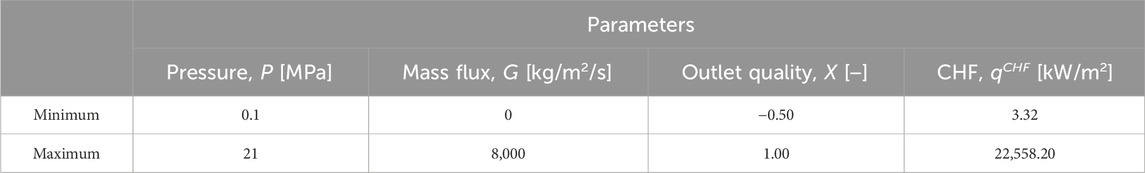
Table 1. Parameter ranges of the empirical (data-driven) Groeneveld Look-Up Table (LUT) (Groeneveld et al., 2007; Groeneveld, 2019).

4.1.2 The mechanistic physics-based Liu model

The mechanistic model developed by Liu et al. (2000), Liu et al. (2012), Liu (2022), Zhao et al. (2020) represents one of the most recent and prominent physics-based approaches for predicting CHF, grounded in the relatively well-established liquid sublayer dryout (DO) mechanism. This model postulates that the onset of Departure from Nucleate Boiling (DNB) occurs due to the complete evaporation of a thin, superheated liquid sublayer situated beneath a vapor blanket adjacent to the heated surface. The vapor blanket itself is assumed to form through the coalescence of vapor bubbles generated near the wall during nucleate boiling. Based on this physical interpretation, a heat balance can be applied to the liquid sublayer, from which a simplified governing equation is derived as ${\widehat{q}}_{Liu}^{CHF}=\left({\rho }_f·\delta {·h}_{fg}/L_B\right){·U}_B$, where: ${\rho }_f$ is the liquid density at saturation and $h_{fg}$ is the latent heat of vaporization; $\delta$, U_B and L_B are respectively the liquid sublayer thickness, vapor blanket velocity, and vapor blanket length. A critical aspect of the liquid sublayer DO mechanism lies in the accurate determination of the three closure terms ($\delta$, U_B and L_B), along with relevant intermediate variables. Multiple models based on the sublayer DO concept have been proposed in the open literature, including the pioneering work by Lee and Mudawwar (1988), the Katto model (Katto, 1990), and the models developed by Celata et al. (1994), (1999), Liu et al. (2000), Liu et al. (2012) and Liu (2022). These models have contributed valuable insights into CHF prediction; however, they also exhibit certain limitations. Among these, the Liu model is one of the most recent and comprehensive developments. It incorporates the effects of hydrodynamic instabilities at both the sublayer-vapor blanket and vapor blanket-bulk flow interfaces, representing a notable advancement in physical realism. Although the fundamental mechanism is theoretically independent of channel geometry, existing closure correlations - including those used in the Liu model - have been primarily derived and validated for round tubes, which restricts their generalizability to other geometries. In a comparative study involving over 2400 CHF test cases in round tubes, Liu et al. (2000) demonstrated that their model offered marginally improved predictive performance relative to the earlier Celata models, highlighting its potential as a more accurate mechanistic tool within its validated domain.

Notice that different from (Zhao et al., 2020), for the implementation of PENNs the improved mechanistic physics-based model presented in Liu et al. (2012) is here adopted instead of the one included in Liu et al. (2000). The model takes into account the microscopic bubble dynamics and integrates it within the liquid sublayer DO mechanism investigated in previous literature works (Liu et al., 2000). The forces exerted on the vapor blankets are duly considered to determine the liquid sublayer thicknesses and relative velocities of the vapor blankets through force balances in the radial and axial direction, respectively. It is worth noting that the referthan Liu model (Liu et al., 2000) was developed for DNB, which usually occurs in the subcooled and low-quality region: coherently, it was validated on 2,482 data characterized by outlet quality X ranging only between −0.6 and 0. Instead, the improved model is demonstrated to perform better that the original one in a wider range of thermodynamic conditions, as verified on 2,587 experimental data from both the subcooled and saturated flow boiling regions (the outlet quality X ranges between −0.4 and 1.0) (Table 2). In detail, the new model shows a lower bias and a higher precision (i.e., lower dispersion): the mean values of the ratio of the predicted to experimental CHF values (namely, ${\widehat{q}}^{CHF}/q^{CHF}$) are 0.966 and 0.746, while the corresponding standard deviations are 0.191 and 0.389 in Liu et al. (2012), Liu et al. (2000), respectively. Also, 85.9% of the data are predicted by Liu et al. (2012) within ±30% error band, while this number falls to 51.3% for the original model (Liu et al., 2000).

Table 2

Table 2. Parameter ranges of the mechanistic physics-based Liu model (Liu et al., 2000; Liu et al., 2012).

4.2 Physics-enhanced neural network (PENN) strategies employed

The empirical (data-based) Groeneveld Look-Up Table (LUT) (Groeneveld et al., 2007; Groeneveld, 2019) and the improved mechanistic physics-based Liu model (Liu et al., 2012) are used in two different ways to incorporate the available background knowledge and physical principles within data-driven NN-based strategies:

1. They are taken as fixed-structure (prior) baseline models, which serve as reference solutions. Then, NN models are employed to capture unknown, unexplored information from the mismatch (i.e., the residuals) between the real CHF values and the estimates produced by the knowledge-based and physical models. The approach has been proposed by Zhao et al. (2020), but it has been coupled with the original Liu model (Liu et al., 2000) and tested on a different, smaller dataset with respect to the one of the present article (actually, the tube geometry and inlet conditions for the present database are in a wider and more extreme parameter range, particularly with respect to the outlet quality X and flow boiling conditions, both subcooled and saturated). The approach is hereafter referred to as Res-PENN (Section 4.2.1).

2. The reference models (i.e., LUT and improved Liu) are directly integrated into the NN loss function definition for effective (physics- and data-driven) training. In this way, domain knowledge-based physics principles guide the learning process, so that the model’s predictions are consistent with the physical principles underlying the phenomena and the corresponding body of knowledge. In other words, the network learns from the data, while at the same time obeying the constraints imposed by the prior, fixed-structure reference models (Section 4.2.2).

4.2.1 Residual-based physics-enhanced neural network (Res-PENN)

In the Residual-based Physics-Enhanced Neural Network (Res-PENN) approach proposed by Zhao et al. (2020), machine learning (i.e., the NN) compensates for biases in classical domain knowledge- or physics-based models and discerns information from the discrepancy between target values and those predicted by reference models. As depicted in Figure 1, during both the training and testing stages of Res-PENN, a conventional knowledge-based, physical or mathematical model g(z), such as the Groeneveld LUT (Groeneveld et al., 2007; Groeneveld, 2019) or the mechanistic physics-based Liu model (Liu et al., 2000; Liu et al., 2012), is selected to represent the “prior” knowledge in the field, or Domain Knowledge (DK) (Zhao et al., 2020). Rather than computing the target value directly, the NN is employed to estimate the disparity (or discrepancy, residual) between the actual target (experimental) value and the prediction from the foundational model. For instance, in a typical CHF study, an input vector z often comprises key thermal fluid quantities like pressure (P), mass flux (G), equilibrium quality (X), channel hydraulic diameter (D), inlet subcooling (Δh_in), inlet temperature (T_in). This vector z is processed by the prior model $g\left(·\right)$ to yield a predicted output ${\widehat{q}}_{Phys}^{CHF}\left(\mathit{z}\right)=g\left(\mathit{z}\right)$. Notice that in this paper ${\widehat{q}}_{Phys}^{CHF}\left(\mathit{z}\right)$ may stand for ${\widehat{q}}_{LUT}^{CHF}\left(\mathit{z}\right)$ or ${\widehat{q}}_{Liu}^{CHF}\left(\mathit{z}\right)$, depending on the baseline model adopted (i.e., LUT or improved Liu, respectively). The error (residual) $\epsilon \left(\mathit{z}\right)=q^{CHF}-{\widehat{q}}_{Phys}^{CHF}\left(\mathit{z}\right)$ is the difference between the actual/measured CHF value $q^{CHF}$ and ${\widehat{q}}_{Phys}^{CHF}\left(\mathit{z}\right)$. At the training stage (Figure 1), an NN is trained with the residuals $\epsilon \left(\mathit{z}\right)$, i.e., it is trained to map the input z to the discrepancy $\epsilon \left(\mathit{z}\right)$ between the experimental and the model-based CHF values. The dataset used to build the model is thus D_build = $\left\{\left({\mathit{z}}_i,{\epsilon }_i=\epsilon \left({\mathit{z}}_i\right)=q_i^{CHF}-{\widehat{q}}_{Phys}^{CHF}\left({\mathit{z}}_i\right)\right),i=1,2,\dots ,N_{build}\right\}$ (which is possibly split into a training and validation set to monitor the NN performance during training and avoid overfitting through early stopping, D_train = $\left\{\left({\mathit{z}}_j,{\epsilon }_j=\epsilon \left({\mathit{z}}_j\right)=q_j^{CHF}-{\widehat{q}}_{Phys}^{CHF}\left({\mathit{z}}_j\right)\right),j=1,2,\dots ,N_{train}\right\}$ and D_val = $\left\{\left({\mathit{z}}_k,{\epsilon }_k=\epsilon \left({\mathit{z}}_k\right)=q_k^{CHF}-{\widehat{q}}_{Phys}^{CHF}\left({\mathit{z}}_k\right)\right),k=1,2,\dots ,N_{val}\right\}$, respectively). During training/validation, the NN-predicted residual (${\widehat{\epsilon }}_i^{NN}={\widehat{\epsilon }}^{NN}\left({\mathit{z}}_i\right)$) is compared with ${\epsilon }_i=\epsilon \left({\mathit{z}}_i\right)$ through a loss (or cost) function. The objective of the training process is to optimize (minimize) the loss function, usually presented as the mean squared error (MSE) or the mean absolute error (MAE). The performance of the final predicted output ${\widehat{q}}_{Res-PENN}^{CHF}\left(\mathit{z}\right)$, i.e., the sum of the reference model CHF prediction ${\widehat{q}}_{Phys}^{CHF}\left(\mathit{z}\right)$ (${\widehat{q}}_{i,Phys}^{CHF}={\widehat{q}}_{Phys}^{CHF}\left({\mathit{z}}_i\right),i=1,2,\dots ,N_{build}=N_{train}+N_{val}$) and the NN-based residual prediction ${\widehat{\epsilon }}^{NN}\left(\mathit{z}\right)$ (${\widehat{\epsilon }}_i^{NN}={\widehat{\epsilon }}^{NN}\left({\mathit{z}}_i\right),i=1,2,\dots ,N_{build}=N_{train}+N_{val}$), is evaluated against the experimental CHF $q^{CHF}$ ($q_i^{CHF},i=1,2,\dots ,N_{build}=N_{train}+N_{val}$). Similarly, at the test stage (Figure 1), the prior domain knowledge-based model and NNs are combined to determine the predicted output for a test set D_test = $\left\{\left({\mathit{z}}_l,q_l^{CHF}\right),l=1,2,\dots ,N_{test}\right\}$ previously left out during training/validation. It should be noted that Figure 1 only shows one of the potential ways how the background knowledge and/or physics could be encoded into the learning process. Other methods, for example, involve hard-coding boundary conditions for the training domain or integrating residuals of conservation laws into the loss function (see Section 4.2.2).

Figure 1

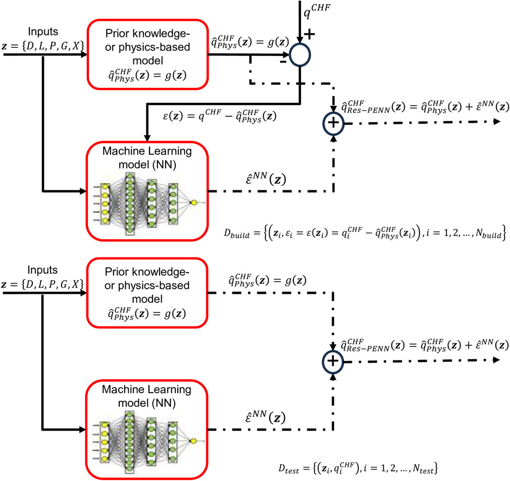
Figure 1. Conceptual structure for the Residual-based Physics-Enhanced Neural Network (Res-PENN) framework during (A) training/validation (top) and (B) testing phases (bottom).

4.2.2 Hybrid loss function-based physics-enhanced neural network (HLF-PENN)

Hybrid Loss Function-based Physics-Enhanced Neural Networks (HLF-PENNs) represent a novel class of modeling frameworks that combine the predictive capabilities of modern machine learning with the rigor of classical physical laws and/or background domain knowledge on the physical phenomena of interest. The primary objective of HLF-PENNs is to embed well-established physical principles directly into the Neural Network (NN) training process, using them as constraints or penalty functions to guide model learning and thereby ensure physically consistent predictions and improved extrapolation performance (Raissi et al., 2019). Unlike conventional data-driven approaches that rely solely on observational data, HLF-PENNs incorporate sound domain knowledge and/or reliable physical laws to inform the learning process, which may also contribute to enhanced interpretability and reduce the likelihood of generating unphysical outputs. By explicitly incorporating reliable knowledge- and/or rigorous physical law-based loss terms, HLF-PENNs tend to yield results that are often more transparent or, at least, aligned with theoretical expectations. It is worth mentioning that HLF-PENNs were originally introduced to address two primary categories of problems: (i) data-driven solutions of Partial Differential Equations (PDEs), and (ii) data-driven discovery of governing PDEs from data. In this framework, NNs are trained not only on data but also under constraints imposed by known physical laws. These laws - typically expressed in the form of PDEs - are embedded into the network’s loss function or imposed as constraints on the outputs, thereby enforcing physical consistency and possibly improving the interpretability of the model predictions (Farea et al., 2024). HLF-PENNs have demonstrated the capability to solve a broad class of differential equations, including classical PDEs, fractional differential equations, integro-differential equations, and stochastic PDEs. A growing body of literature illustrates their successful application across diverse physical domains (Cuomo et al., 2022; De La Mata et al., 2023; Cicirello, 2024). Notable examples include fluid dynamics solutions to the incompressible Navier-Stokes equations (Jin et al., 2021), heat transfer problems (Karpatne et al., 2017; Cai et al., 2021; Jalili et al., 2024), solid and structural mechanics simulations (Diao et al., 2023; Marino and Cicirello, 2023; Yang et al., 2025), and nuclear safety analysis (Antonello et al., 2023; Lai et al., 2024; Lye et al., 2025), highlighting the versatility and expanding relevance of PENNs in computational physics. Finally, it must be noted that while HLF-PENNs are more often associated with dynamic systems described by differential equations, in this work it is applied to a static model description, i.e., the empirical Groeneveld LUT and the improved Liu model.

HLF-PENNs often incorporates sound knowledge-based and rigorous physical constraints, equations and laws into the loss function using a Mean Squared Error (MSE)-like penalty, similar to conventional NNs (Yang L. et al., 2021; Stock et al., 2024; Pensoneault and Zhu, 2024; Ahmed et al., 2025). In other words, the HLF-PENN training is guided by two terms: i) the discrepancy between the NN prediction ${\widehat{q}}_{HLF-PENN}^{CHF}\left(\mathit{z}\right)$ and the experimental data $q^{CHF}$ (namely, the data loss); ii) the difference between the NN estimates ${\widehat{q}}_{HLF-PENN}^{CHF}\left(\mathit{z}\right)$ and the domain knowledge- and mechanistic physics-based model outputs ${\widehat{q}}_{Phys}^{CHF}\left(\mathit{z}\right)$ (namely, the physics-related loss) (Figure 2). Notice that in this paper ${\widehat{q}}_{Phys}^{CHF}\left(\mathit{z}\right)$ can be either ${\widehat{q}}_{LUT}^{CHF}\left(\mathit{z}\right)$ or ${\widehat{q}}_{Liu}^{CHF}\left(\mathit{z}\right)$, depending on the reference (prior) model adopted. The loss term associated with the experimental data available (${\mathcal{L}}_{data}$) is classically defined as in Equation 1:

${\mathcal{L}}_{data}=\frac{1}{N_{train}}{\displaystyle \sum _{i=1}^{N_{train}}}{\left({\widehat{q}}_{HLF-PENN}^{CHF}\left({\mathit{z}}_i\right)-q_i^{CHF}\right)}^2=\frac{1}{N_{train}}{\displaystyle \sum _{i=1}^{N_{train}}}{\left({\widehat{q}}_{i,HLF-PENN}^{CHF}-q_i^{CHF}\right)}^2(1)$

The loss term associated with the knowledge- and mechanistic physics-related residuals (${\mathcal{L}}_{phys}$) relies on the simple difference between the NN predicted CHF and the one calculated with the selected reference (prior) model (i.e., either the LUT or the improved Liu model in this paper), as indicated in Equation 2. This makes sure the learning process goes in the direction of approximating the given reference model as accurately as possible:

${\mathcal{L}}_{phys}=\frac{1}{N_{train}}{\displaystyle \sum _{i=1}^{N_{train}}}{\left({\widehat{q}}_{HLF-PENN}^{CHF}\left({\mathit{z}}_i\right)-{\widehat{q}}_{Phys}^{CHF}\left({\mathit{z}}_i\right)\right)}^2=\frac{1}{N_{train}}{\displaystyle \sum _{i=1}^{N_{train}}}{\left({\widehat{q}}_{i,HLF-PENN}^{CHF}-q_{i,Phys}^{CHF}\right)}^2(2)$

The global (hybrid) loss function is then defined by weighing contributions (1) and (2) above by means of another hyperparameter λ to be optimized through validation and it is defined as in the following Equation 3 (Figure 2):

${\mathcal{L}}_{total}={\left(1-\lambda \right)\mathcal{·}\mathcal{L}}_{data}+{\lambda \mathcal{·}\mathcal{L}}_{phys}(3)$

After training, which proceeds exactly as for classical NNs, the system has learnt how to approximate the CHF across the defined domain.

Figure 2

Figure 2. Conceptual structure of the Hybrid Loss Function-based Physics-Enhanced Neural Network (HLF-PENN).

A final word of caution is in order with respect to the (possibly increased) “interpretability” of our HLF-PENN model with respect to pure data-driven NN approaches. On the one hand, an argument for higher interpretability could be made by the inclusion of the improved mechanistic Liu model in the loss function (3) (i.e., when ${\widehat{q}}_{Phys}^{CHF}\left(\mathit{z}\right)$ = ${\widehat{q}}_{Liu}^{CHF}\left(\mathit{z}\right)$). Actually, although imperfect, this model relies on relatively well-known and transparent physics-based concepts, correlations and equations, which may be easy to understand by the user and may reduce the amount of inferred (purely data-based) knowledge required by the ML component. On the other hand, it must be acknowledged that in this paper the NN loss function (3) is not regularized with first-principle physical laws (e.g., PDEs representing the “ground truth” for the phenomena of interest). Rather, imperfect prior models are employed that have no absolute guarantee to carry out correct (i.e., “true” or “perfect”) predictions in all the regions of the input space: in this view, as mentioned above, the hybrid regularized training of the HLF-PENNs here developed only ensures additional “pressure” towards the (imperfect) model outputs available (which is still of paramount importance in the presence of very scarce, uncertain, noisy or unreliable data).

4.3 Uncertainty quantification on CHF predictions by bootstrapped PENN ensembles

When employing the approximation of system outputs generated by a PENN empirical regression model, additional sources of uncertainty are introduced, which must be carefully assessed - particularly in safety-critical domains such as nuclear power plant technology. These uncertainties primarily arise from three key factors:

a. The set D_build (= D_train $\cup$ D_val) adopted to build the network is inherently limited in scope due to the finite number of available input/output data samples. As a result, this dataset cannot comprehensively span the entire input domain of interest. Therefore, different datasets D_build may lead to different internal network parameters and regression functions, giving rise to an empirical distribution of possible regression models.

b. The selection of the network architecture itself may be suboptimal. For instance, choosing an inappropriate number of hidden neurons - either too few or too many - can impair the model’s generalization capability. A balance between model complexity and generalization can be achieved by managing the number of parameters and adopting appropriate training strategies, such as early stopping (Zio, 2006).

c. Once trained, neural networks behave as deterministic functions, yielding identical outputs for repeated evaluations of the same input. However, when multiple networks are independently trained - differing in aspects such as weight initialization, hyperparameters, or optimization procedures - they often produce slightly different outputs for the same input. These variations can be interpreted as samples from an underlying predictive distribution, facilitating uncertainty quantification. Additionally, convergence to a global minimum of the loss function is not guaranteed during training. Optimization algorithms may converge to suboptimal local minima or may be halted prematurely before reaching a satisfactory error threshold (Zio, 2006; Furlong et al., 2025a). These aspects introduce further uncertainty that must be accounted for when assessing the reliability and robustness of neural network-based predictions.

Thus, due to the uncertainties, for given model input parameters/variables, the model output (i.e., the CHF prediction) can vary within a range of possible values (e.g., within a Prediction Interval-PI) (Efron and Tibshirani, 1994). The uncertainty described in item a) above is related to the limited size of the (possibly noisy) dataset and is here quantified by bootstrapping (Efron and Thibshirani, 1994). This approach can quantify the uncertainty by considering an ensemble of PENNs built on B different data sets that are sampled with replacement (bootstrapped) from the original one (Zio, 2006). From each bootstrap data set $D_{build}^b$, b = 1, 2, … , B, a bootstrapped PENN regression model is built, and the model output of interest can be computed, ${\widehat{q}}^{CHF,b}\left(\mathit{z}\right)$, b = 1, 2, … , B. In this work, B = 100 is chosen. The use of multiple bootstrap datasets leads to an empirical distribution of regression functions, thereby enabling the construction of a probability density function (PDF) for the model output. This allows the uncertainty associated with the predictions generated by PENNs to be quantitatively assessed - for example, through the derivation of prediction intervals from the output PDF produced via the bootstrap procedure. A key advantage of this method is that it provides prediction intervals for a given model output without requiring strong assumptions about the underlying distribution (e.g., normality). Furthermore, both theoretical insights and empirical evidence from ensemble modeling suggest that the aggregated predictions obtained from bootstrapped regression models generally exhibit higher accuracy than those produced by any single model within the ensemble (Zio, 2006; Pedroni et al., 2010; Zio et al., 2010). Nonetheless, this approach can incur significant computational costs, particularly when dealing with large training datasets or models with a high number of parameters (Pedroni et al., 2010; Zio et al., 2010). Instead, the uncertainty described in items b) and c) is associated with the model architecture, (random) hyperparameters initialization and optimization. The simplest way of quantifying such (model) uncertainty is again that of a PENN ensemble created by an initialization-based strategy. In this paper, for each bootstrapped model b = 1, 2, … , B (= 100), a set of S (= 20) models is trained using different weight/bias (random) starting values (Yaseen and Wu, 2023; Tan et al., 2023; LeCun et al., 2015; Furlong et al., 2025a): each of these models, s = 1, 2, … , S, explores a different portion of the solution space to find a global minimum of the objective function. At the end of the overall ensemble training, for a given input vector z, a (probability) distribution of B·S (output) CHF predictions is obtained as ${\widehat{q}}^{CHF,b,s}\left(\mathit{z}\right)$, b = 1, 2, … , B, s = 1, 2, … , S, which encompasses all the forms of uncertainty a), b) and c) mentioned above. To avoid that the CHF distributions thereby obtained are biased by outliers (possibly resulting from errors and badly trained models), “extreme” PENN predictions are discarded: in particular, we eliminate CHF values falling outside the interval obtained by extending below and above the lower and upper quartiles, respectively, by 1.5 times the interquartile range. Finally, the mean value of such distribution $1/\left(B·S\right)·{\displaystyle \sum _{b=1}^B}{\displaystyle \sum _{s=1}^S}{\widehat{q}}^{CHF,b,s}\left(\mathit{z}\right)$ is used as the ensemble’s “single-value” prediction ${\widehat{q}}^{CHF}\left(\mathit{z}\right)$ in further analyses. With respect to the quantification of uncertainty, the use of bootstrapped ensembles produces an empirical (probability) distribution of (output) CHF predictions, from which Prediction Intervals (PIs) (with confidence level $\left(1-\gamma \right)$) can be identified as follows. In this paper, the two-sided 100(1 – γ)% prediction interval for the CHF prediction ${\widehat{q}}^{CHF}$ is computed by ordering the estimates ${\widehat{q}}^{CHF,b,s}$, b = 1, 2, … , B, s = 1, 2, … , S, in increasing values and identifying the (100γ/2)-th and 100(1 – γ/2)-th quantiles of the bootstrap-based empirical PDF as the closest values to the (B·S·γ/2)-th and B·S·(1 – γ/2)-th elements, respectively. In the following, the prediction interval of ${\widehat{q}}^{CHF}$ is referred to as $\left[{\underset{\_}{q}}^{CHF,100\left(1-\gamma \right)\%},{\overline{q}}^{CHF,100\left(1-\gamma \right)\%}\right]$. Finally, it is worth clarifying that PIs reflect the confidence in where a new prediction of a given input combination will fall, which is indicative of the underlying (empirical) distribution (of CHF predictions): as such, (the widths of) PIs do not change with increased samples (B and/or S). Instead, Confidence Intervals (CIs) reflect confidence in where the mean value of the ensemble lies, and they shrink as more samples (B and/or S) are taken (Efron and Tibshirani, 1994).

4.4 Performance metrics

A combination of more than one statistical measure is used to comprehensively assess the proposed PENN models’ performance. The following metrics, commonly used in the nuclear engineering sector and suggested by Le Corre et al. (2024), are employed to assess the performance of the proposed method on the training, validation and test datasets, D_train = $\left\{\left({\mathit{z}}_j,q_j^{CHF}\right),j=1,2,\dots ,N_{train}\right\}$, D_val = $\left\{\left({\mathit{z}}_k,q_k^{CHF}\right),k=1,2,\dots ,N_{val}\right\}$ and D_test = $\left\{\left({\mathit{z}}_l,q_l^{CHF}\right),l=1,2,\dots ,N_{test}\right\}$, respectively, and on their combination, i.e., D_data = D_train $\cup$ D_val $\cup$ D_test = D_build $\cup$ D_test = $\left\{\left({\mathit{z}}_i,q_i^{CHF}\right),i=1,2,\dots ,{N_{data}=N_{train}+N_{val}+N}_{test}\right\}$. For brevity, the quantitative performance metrics are written only with reference to D_data:

⁃ the relative Root Mean Squared Percentage Error (rRMSPE), calculated as in Equation 4:

$rRMSPE=100·\sqrt{\frac{1}{N_{data}}{\displaystyle \sum _{i=1}^{N_{data}}}{\left(\frac{q_i^{CHF}-{\widehat{q}}_i^{CHF}}{q_i^{CHF}}\right)}^2}(4)$

⁃ the relative Mean Absolute Percentage Error (rMAPE), computed as in Equation 5:

$rMAPE=100·\frac{1}{N_{data}}{\displaystyle \sum _{i=1}^{N_{data}}}\left|\frac{q_i^{CHF}-{\widehat{q}}_i^{CHF}}{q_i^{CHF}}\right|(5)$

⁃ the normalized Root Mean Squared Percentage Error (nRMSPE), defined in Equation 6 as the RMSE divided by the estimated mean value of the (output) dataset ${\overline{q}}^{CHF}$ (Grosfilley, 2022):

$nRMSPE=100·\frac{\sqrt{\frac{1}{N_{data}}{\displaystyle {\sum }_{i=1}^{N_{data}}}{\left(q_i^{CHF}-{\widehat{q}}_i^{CHF}\right)}^2}}{{\overline{q}}^{CHF}}=100·\frac{\sqrt{\frac{1}{N_{data}}{\displaystyle {\sum }_{i=1}^{N_{data}}}{\left(q_i^{CHF}-{\widehat{q}}_i^{CHF}\right)}^2}}{\frac{1}{N_{data}}{\displaystyle {\sum }_{i=1}^{N_{data}}}{q}_i^{CHF}}(6)$

⁃ the Q²-error, evaluated as in Equation 7:

$Q^2=100·\frac{{\displaystyle {\sum }_{i=1}^{N_{data}}}{\left({\widehat{q}}_i^{CHF}-q_i^{CHF}\right)}^2}{{\displaystyle {\sum }_{i=1}^{N_{data}}}{\left(q_i^{CHF}-{\overline{q}}^{CHF}\right)}^2}=100·\frac{{\displaystyle {\sum }_{i=1}^{N_{data}}}{\left({\widehat{q}}_i^{CHF}-q_i^{CHF}\right)}^2}{{\displaystyle {\sum }_{i=1}^{N_{data}}}{\left(q_i^{CHF}-\frac{1}{N_{data}}{\displaystyle {\sum }_{o=1}^{N_{data}}}{q}_i^{CHF}\right)}^2}(7)$

The relative percentage RMSE ($rRMSPE$) (4) quantifies the prediction error as a percentage of the actual (measured) values, thereby enabling a scale-independent assessment of model accuracy. This makes rRMSPE particularly valuable in applications involving large datasets with significant variability in the magnitude of measured values, as it facilitates meaningful comparisons of predictive performance across different data scales. However, $rRMSPE$ is sensitive to extreme data points, penalizing typically larger errors and predictions of small CHF values ($q_i^{CHF}$). To mitigate this effect, the $rRMSPE$ has been accompanied by the nRMSPE (6), where the RMSE is normalized by the mean value ${\overline{q}}^{CHF}$ of the entire dataset (Grosfilley, 2022). The rMAPE (5) also offers a clear and intuitive interpretation, as it directly reflects the average percentage error across all predictions. By expressing the error as a percentage of the actual values, rMAPE provides an easily interpretable measure of model accuracy, allowing for an immediate understanding of the error magnitude relative to the true data. Indicator Q² (7) evaluates the squared error discrepancies normalized by the variance of the observed data, effectively quantifying the proportion of data variability explained by the model. There may be situations where the RMSE is small (i.e., the numerator of Q² is small), and the variance of the dataset (i.e., the denominator) presents also a small value: in such a case, the Q² metric may turn out to present disproportionately high values. In other words, the indicator Q² evaluates how well a regression model’s prediction reflects actual data values and provides a relative assessment of the model predictive capability, considering the variability in the data. Values close to 0 indicate strong predictive capabilities, while values greater than 1 suggest worse predictive capabilities than simply using mean value as its prediction (Le Corre et al., 2024). Other indicators suggested by Le Corre et al. (2024) are the mean and the standard deviation of the distribution of the ratios of the predicted (P) over measured (M) CHF values, respectively, i.e.,:

$\widehat{PM}=\frac{1}{N_{data}}{\displaystyle \sum _{i=1}^{N_{data}}}\frac{{\widehat{q}}_i^{CHF}}{q_i^{CHF}}(8)$

$\widehat{\sigma }\left(PM\right)=\sqrt{\frac{1}{N_{data}-1}{\displaystyle \sum _{i=1}^{N_{data}}}{\left(\frac{{\widehat{q}}_i^{CHF}}{q_i^{CHF}}-\widehat{PM}\right)}^2}(9)$

The mean value $\widehat{PM}$ of Equation 8 measures whether the model is biased. If such mean value deviates from one significantly, the model has probably not found the right fit. The standard deviation $\widehat{\sigma }\left(PM\right)$ of Equation 9 measures by construction the proportional error/discrepancy and the dispersion of the ML model. A similar indication can be obtained by computing the amount of data points falling within a specific (relative) error threshold α% (in this paper, α = 10 and 20 are considered), as in Equation 10:

$E_{\alpha \%}=\frac{1}{N_{data}}·\#\left\{100·\left|\frac{q_i^{CHF}-{\widehat{q}}_i^{CHF}}{q_i^{CHF}}\right|\le \alpha \%\right\}(10)$

The quantitative indicators above are used for hyperparameters optimization and ensemble (NN and PENN) model construction and evaluation. All the comparisons are carried out employing the early stopping method to avoid overfitting and guarantee satisfactory generalization capabilities to new (test) data (i.e., not employed during model construction).

With respect to the quantification of uncertainty, the use of bootstrapped ensembles produces a $100\left(1-\gamma \right)\%$ prediction interval for each CHF prediction ${\widehat{q}}_i^{CHF}$, i = 1, 2, … , N_data, indicated as $\left[{\underset{\_}{q}}_i^{CHF,100\left(1-\gamma \right)\%},{\overline{q}}_i^{CHF,100\left(1-\gamma \right)\%}\right]$. To determine the quality of the prediction intervals, two quantitative measures can be taken into account (Ak et al., 2013; Ferrario et al., 2017): the Coverage Probability (CP) and the Normalized Mean Width (NMW). The former represents the probability that the true values of the CHF ($q_i^{CHF}$, i = 1, 2, … , N_data) are included in the corresponding prediction intervals, whereas the latter quantifies the extension of the prediction intervals and it is usually normalized with respect to the minimum and maximum of the patterns used to build the NN model, i.e., the union of the training and validation datasets ($D_{build}=D_{train}$ $\bigcup$ $D_{val}$ = {$q_i^{CHF}$: i = 1, 2, … , N_train + N_val}). They are typically conflicting measures, since the larger NMW the larger CP, while in practice it is important to have large coverage (i.e., a large fraction of the experimental data “explained” by the model) and small width (i.e., small uncertainty in the model predictions). The CP (Equation 11) is given by Ak et al. (2013), Ferrario et al. (2017):

$CP=\frac{1}{N_{data}}{\displaystyle {\sum }_{i=1}^{N_{data}}}{p}_i(11)$

where $p_i=1$, if $q_i^{CHF}$ ∈ $\left[{\underset{\_}{q}}_i^{CHF,100\left(1-\gamma \right)\%},{\overline{q}}_i^{CHF,100\left(1-\gamma \right)\%}\right]$; otherwise $p_i=0$, for i = 1, 2, … , N_data. In this paper, $\gamma$ = 0.05 is selected. A (regression) model can be considered statistically validated, if for a value of $\gamma$ selected by the analyst (i.e., for a desired level of confidence) the empirical CP results to be larger than or equal to (1 – $\gamma$), i.e., if at least the (1 – $\gamma$)·100% of the data points are actually covered by (i.e., included in) the PIs. The NMW (Equation 12) is computed as (Ak et al., 2013; Ferrario et al., 2017):

$NMW=\frac{1}{N_{data}}{\sum }_{i=1}^{N_{data}}\frac{\left[{\overline{q}}_i^{CHF,100\left(1-\gamma \right)\%}-{\underset{¯}{q}}_i^{CHF,100\left(1-\gamma \right)\%}\right]}{q_{\mathit{max}}^{CHF}-q_{\mathit{min}}^{CHF}}(12)$

where $q_{i,\mathit{max}}^{CHF}$ and $q_{i,\mathit{min}}^{CHF}$ are the maximum and minimum values of the CHF within the (validation and training) dataset used to build the ANN models, respectively. Since each PIs is indicative and descriptive of the (spread of the) empirical probability distribution of the corresponding CHF prediction (Section 4.3), then the NMW is a synthetic indicator of the average uncertainty associated with the model predictions, over the entire dataset available: the smaller the NMW, the smaller the (average) spread (i.e., the uncertainty) of the underlying CHF prediction distributions, the higher the precision of the model estimates. Normalization by ($q_{i,\mathit{max}}^{CHF}$ − $q_{i,\mathit{min}}^{CHF}$) is required when non commensurable quantities need to be compared (in the present case, it may not be mandatory).

5 Case study: the U.S. nuclear regulatory commission (NRC) CHF database

The present study employs the Critical Heat Flux (CHF) dataset compiled by the U.S. Nuclear Regulatory Commission (NRC), as documented in Groeneveld (2019), to train, validate, and test the proposed Physics-Enhanced Neural Network (PENN)-based predictive models. This dataset represents the largest publicly available compilation of CHF measurements, comprising 24,579 individual data points collected from 59 distinct experimental sources. Each entry corresponds to a CHF measurement obtained in a vertically oriented, water-cooled, uniformly heated tube subjected to varying experimental conditions. The majority of CHF values were identified using thermocouples positioned to detect rapid temperature excursions indicative of CHF onset. The dataset includes a comprehensive parameter space encompassing boundary conditions and geometric variables, as detailed in Table 3. Input features used for neural network modeling are categorized as follows: (i) geometric parameters (tube diameter D, heated length L); (ii) directly measured parameters (pressure P, mass flux G, inlet temperature T_in); and (iii) calculated parameters (outlet quality X, inlet subcooling Δh_in), both calculated from water saturation properties. Although the NRC CHF dataset covers a wide and diverse range of the parameter space, it should be noted that the distribution of data points is not uniform across all variables. In particular, no data points exist for tube diameters greater than 16 mm. While the NRC dataset closely aligns with the database used in the development of the 2006 CHF LUT, all proprietary or non-public data have been excluded from the version used here (Groeneveld, 2019). Additionally, rigorous data preprocessing was undertaken to identify and eliminate non-physical entries, outliers, and duplicate records, as recommended in previous literature (Groeneveld, 2019; Groeneveld et al., 2007).

Table 3

Table 3. Parameters range for the USNRC CHF dataset (Groeneveld, 2019).

Figure 3 shows a scatter plot matrix of the NRC CHF dataset points to get an overview of the ranges with large amount of data availability (and thus providing higher reliability when modelled) and those lacking experimental points. Also, Figure 3 shows scatter plots highlighting the relationships between CHF and each input parameter. This allows for the evaluation of potential relationships between variables and the assessment of data distribution, as well as the study of possible input-output relationships. The CHF prediction can be made using all these input parameters (Ahmed et al., 2025) or, more often, by resorting to a properly selected subset. In this work, three different input sets are first considered to assess the predictive capability of a standalone (basic) NN model (Grosfilley et al., 2024): i) $\left\{D,L,P,G,X\right\}$; ii) $\left\{D,L,P,G,T_{in}\right\}$; iii) $\left\{D,L,P,G,\Delta h_{in}\right\}$. Then, the extensive comparison between all the PENN strategies mentioned above is carried out with reference to input configuration $\left\{D,L,P,G,X\right\}$. This selection is based on several considerations: (i) currently, most CHF prediction models for convective boiling systems use analytical functions that mainly depend on these physical quantities (Le Corre et al., 2024; Grosfilley et al., 2024); (ii) the Challengers leading the “Task Force on Artificial Intelligence and Machine Learning for Scientific Computing in Nuclear Engineering” explicitly require training and evaluation (validation and test, including extrapolation) of ML regression models on the Groeneveld dataset using these five parameters as inputs; (iii) as pointed out in Grosfilley (2022), Grosfilley et al. (2024), using T_in (or $\Delta h_{in}$) often give better results. However, it is worth highlighting that these models (based on inlet conditions) must be used with caution, since their validity depends on a simple heat balance being upheld for isolated subchannels. This assumption can be false when dealing with more complex geometries, crossflow, non-uniform heating and fast transients (such as in fuel bundles): in these cases, the usage of an input set based on local conditions (e.g., local outlet quality) is recommended.

Figure 3

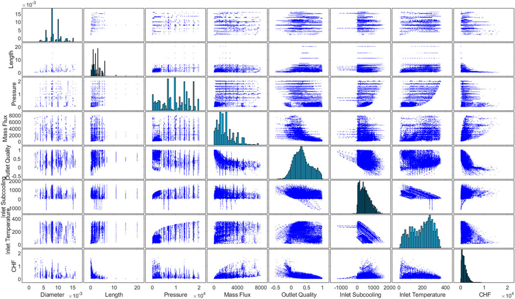
Figure 3. Scatter plot matrix of the NRC CHF database (Groeneveld, 2019) showing the relationship between pairs of variables.

6 Results

In this section, the performances of the different PENNs models are assessed. In Section 6.1, the Res-PENNs and HLF-PENNs (based on both the LUT and the improved Liu models) are trained using the entire large NRC CHF dataset (24,579 points) and compared to purely data-driven NNs. In Section 6.2, the capability of PENNs to perform accurate and precise CHF predictions in the presence of very scarce data (e.g., a few tens or hundreds of training patterns) is systematically tested. Finally, in Section 6.3, the uncertainty associated with the CHF estimates provided by the standalone NNs and PENNs is estimated by bootstrapped ensembles and random weights reinitialization.

6.1 Performance of PENNs trained on the entire USNRC CHF dataset

The PENN performances are compared to the following references: i) the standalone empirical LUT (Section 4.1.1) and the improved mechanistic physics-based Liu (Section 4.1.2) models; and ii) purely data-driven ensemble NN models. The synthetic indicators described in Section 4.4 are summarized in Table 4 for the LUT and Liu models. As highlighted also in Zhao et al. (2020), the LUT performs in general slightly better than the Liu model: this is particularly evident with respect to the rMAPE, nRMSPE, Q², $E_{10\%}$ and $E_{20\%}$ indicators. On the contrary, the Liu model presents smaller rRMSPE and $\widehat{\sigma }\left(PM\right)$, while both models show a non-negligible bias: in particular, the LUT (resp., Liu) model overestimates (resp., underestimates) the CHF by approximately 3.20% (resp., 4.29%). Notice that the results obtained for the improved Liu model are coherent with those reported in the original paper by Liu et al. (2012).

Table 4

Table 4. Performance metrics (Section 4.4) calculated for the standalone empirical LUT (Groeneveld et al., 2007; Groeneveld, 2019) and the improved mechanistic physics-based Liu model (Liu et al., 2000; Liu et al., 2012) on the entire USNRC CHF dataset.

With respect to the NN regression models, in the present case study the number of inputs is equal to M = 5, whereas the number of outputs is equal to 1 (i.e., the CHF). The network structure, i.e., the number of hidden layers and the number of nodes in each hidden layer (see Table 5), has been optimally identified by grid search (Zio, 2006; Chicco, 2017): the interested reader is referred to (Castrignanò, 2025) for details, since the NN structure optimization does not represent the main purpose of the paper. It is only worth mentioning that for the regression task to be fair, as a rough guideline, each NN architecture is such that the overall number of internal weights and adjustable parameters does not exceed the number of patterns used to build the model (i.e., N_build = N_train $+$ N_val). Sigmoidal activation functions are used for the hidden neurons; instead, given the nature of the problem, the rectified linear unit (ReLU) is selected for the output neuron, which avoids negative values of CHF predictions. The entire USNRC CHF dataset is split into two subsets, the first (D_build = D_train $\bigcup$ D_val, including 87.5% of the points, i.e., 21,506) to build the NNs, and the second (D_test, including 12.5% of the points, i.e., 3,073) to test the performance of the constructed models on unseen data (i.e., data not used during ANN model construction), D_test = $\left\{\left({\mathit{z}}_i,q_i^{CHF}=y_i\right),i=1,2,\dots ,N_{test}=3073\right\}$. In more detail, model training and validation are carried out by means of the k-fold cross validation method. This method separates D_build = D_train $\bigcup$ D_val into k folds (in this paper, k = 5); then, one fold (thus constituted by 17.5% of the data points from the overall USNRC CHF dataset) is used for validation (D_val = $\left\{\left({\mathit{z}}_i,q_i^{CHF}=y_i\right),i=1,2,\dots ,N_{val}=4301\right\}$) and the others (representing the 70% of all the instances available) for training (D_train = $\left\{\left({\mathit{z}}_i,q_i^{CHF}=y_i\right),i=1,2,\dots ,N_{train}=17205\right\}$). This process is repeated k (=5) times, where each fold is sequentially used as the validation set while the remaining folds are employed for training. This process is repeated until each fold has served as the validation set exactly once. For each iteration, the performance of the NN is evaluated on the corresponding validation set in terms of accuracy (for classification) or regression error (for regression tasks). The overall performance metric - accuracy or regression error - is then computed as the average across all k folds. To track the average performance of the NN models throughout training and to mitigate overfitting, an early stopping strategy is applied. This mechanism halts training if no improvement is observed in the best recorded average validation loss over a patience window of 50 iterations. Regardless, the maximum number of training epochs is capped at 5,000. In the context of this regression task, the MSE is employed as the loss function, which is minimized using the scaled conjugate gradient backpropagation algorithm. The ensemble is made of B = 100 bootstrapped NN models (constructed by random sampling with replacement of the overall training and validation data, D_build = D_train $\bigcup$ D_val) and S = 20 random initializations of the NN weights and biases.

Table 5

Table 5. Performance metrics (Section 4.4) obtained by purely data-driven NN ensembles (B = 100, S = 20) on the entire USNRC CHF dataset, in correspondence of three input sets $\left\{D,\mathit{ln}\left(L\right),\mathit{ln}\left(P\right),\mathit{ln}\left(G\right),X\right\}$, $\left\{D,\mathit{ln}\left(L\right),\mathit{ln}\left(P\right),\mathit{ln}\left(G\right),T_{in}\right\}$ and $\left\{D,\mathit{ln}\left(L\right),\mathit{ln}\left(P\right),\mathit{ln}\left(G\right),\Delta h_{in}\right\}$.

As mentioned above, three different input sets are first considered to assess the predictive capability of a standalone (basic) NN model (Grosfilley et al., 2024): i) $\left\{D,L,P,G,X\right\}$; ii) $\left\{D,L,P,G,T_{in}\right\}$; iii) $\left\{D,L,P,G,\Delta h_{in}\right\}$. More precisely, it is found that taking the natural logarithm (ln) of L, P, G and of the output CHF (to reduce the relative magnitude and produce data points that are more evenly distributed in their respective ranges), greatly improves the NN performances: details can be found in Castrignanò (2025) by the interested reader. Also, given the scale differences across the 5 input variables, data scaling (a recommended pre-processing step for all ML algorithms) is implemented to make the inputs commensurable. The ln-transformed data are thus scaled within the range [−1, +1] by Min-Max normalization function. The results obtained by purely data-driven ensemble NNs with input sets $\left\{D,\mathit{ln}\left(L\right),\mathit{ln}\left(P\right),\mathit{ln}\left(G\right),X\right\}$, $\left\{D,\mathit{ln}\left(L\right),\mathit{ln}\left(P\right),\mathit{ln}\left(G\right),T_{in}\right\}$ and $\left\{D,\mathit{ln}\left(L\right),\mathit{ln}\left(P\right),\mathit{ln}\left(G\right),\Delta h_{in}\right\}$ are reported in Table 5 with respect to all the performance metrics of Section 4.4, computed on the test set D_test = $\left\{\left({\mathit{z}}_i,q_i^{CHF}=y_i\right),i=1,2,\dots ,N_{test}=3073\right\}$ and for completeness on all the N_data = 24579 USNRC data D_data = D_build $\bigcup$ D_test = D_train $\bigcup$ D_val $\bigcup$ D_test, as requested by the Challengers leading the “Task Force on Artificial Intelligence and Machine Learning for Scientific Computing in Nuclear Engineering” (Le Corre et al., 2024). The purely data-driven NN architectures impressively outperform both the reference LUT and Liu models (Table 4) with respect to all the indicators: they are more accurate (lower rRMSPE, rMAPE, nRMSPE), more precise (lower $\widehat{\sigma }\left(PM\right)$, higher $E_{10\%}$ and $E_{20\%}$), less biased ($\widehat{PM}$ closer to 1) and explain better the variability of the dataset (Q² closer to 0). Inputs $\left\{D,\mathit{ln}\left(L\right),\mathit{ln}\left(P\right),\mathit{ln}\left(G\right),T_{in}\right\}$ and $\left\{D,\mathit{ln}\left(L\right),\mathit{ln}\left(P\right),\mathit{ln}\left(G\right),\Delta h_{in}\right\}$ show comparable results and represent the best options. For example, the corresponding percentage improvements with respect to the Liu model range from 4.6% ($\widehat{PM}$) to 234.1% ($E_{10\%}$), with a relative reduction in rRMSPE, rMAPE and Q² of 73.9%–90.2%, 82.3%–86.9% and 98.1%–98.7%, respectively. Considering the LUT, percentage improvements range from 2.8% ($\widehat{PM}$) to 119.5% ($E_{10\%}$), with a relative reduction in rRMSPE, rMAPE and Q² of 66.6%–87.4%, 83.8%–88.0% and 91.0%–93.7%, respectively. It is also important to highlight that in the present application less than 20,000 data points (in particular, N_train = 17205) are sufficient to push the rMAPE to around 2.8%, presumably approaching the average noise boundary of the dataset: this represents an additional strong statement in support of the use of NNs, also when huge datasets (or big data) are not available. Input set $\left\{D,\mathit{ln}\left(L\right),\mathit{ln}\left(P\right),\mathit{ln}\left(G\right),X\right\}$ shows comparably lower but still appreciable performances. Actually, percentage improvements range from 2.5% ($\widehat{PM}$ of LUT) to 156.2% ($E_{10\%}$ of Liu), with a relative reduction in rRMSPE, rMAPE and Q² of 58.6%–68.9%, 60.9%–65.8% and 76.0%–95.6%, respectively. These figures represent very strong statements in favor of: i) the use of AI/ML (and in particular, NNs) for CHF predictions; ii) the accurate selection (and possibly transformation) of relevant physical inputs to feed ML models. Finally, it is worth noting that the results here obtained by classical NNs (Table 5) are at least comparable to (or even better than) those reported in the open literature and produced by more sophisticated algorithms (e.g., Convolutional Neural Networks-CNNs, Transformers, Ensembles of Deep Sparse AutoEncoders, …) with a higher number of inputs and/or more complex structures and architectures (i.e., a much larger number of adjustable parameters) (Zhou et al., 2024; Qi et al., 2025; Grosfilley et al., 2024; Khalid et al., 2024a; Kumar et al., 2024).

Even if using T_in or $\Delta h_{in}$ provides better results, as mentioned above, the extensive comparison between all the PENN strategies is carried out with reference to input configuration $\left\{D,\mathit{ln}\left(L\right),\mathit{ln}\left(P\right),\mathit{ln}\left(G\right),X\right\}$. Most of the relevant reasons for this selection are summarized in Section 5 above (Le Corre et al., 2024; Grosfilley et al., 2024; Grosfilley, 2022); in addition, the results in Table 5 seem to suggest that such input set (i.e., the one performing worse) may obtain relatively higher benefits from the integration with background domain knowledge and physics-based models (i.e., LUT and Liu, respectively), while those including T_in or $\Delta h_{in}$ are already characterized by excellent figures of merit (difficult to improve further). Table 6 shows the performance metrics (Section 4.4) obtained by the Res-PENN ensembles (Sections 4.2.1 and 4.3) on the entire USNRC CHF dataset, using the empirical Groeneveld LUT and the improved Liu as domain knowledge- and mechanistic physics-based reference models, respectively. The results are very promising, since both Res-PENN ensembles significantly improve the performance obtained by the corresponding purely data-driven NN model using the same inputs (Table 5). For example, the corresponding percentage improvements obtained by the LUT-based Res-PENN range from 0.27% ($\widehat{PM}$) to 56.5% (rMAPE), with a relative reduction in rRMSPE, Q² and $\widehat{\sigma }\left(PM\right)$ of 54.4%, 35.5% and 46.8%, respectively. Considering the Liu-based Res-PENN, percentage improvements range from 0.86% ($\widehat{PM}$) to 81.7% (Q²), with a relative reduction in rRMSPE, rMAPE and $\widehat{\sigma }\left(PM\right)$ of 63.4%, 67.4% and 63.5%, respectively. Several important considerations are in order. Within the residual-based framework, the reference model remains fixed throughout both the training and validation phases. The integration of this fixed reference model, whether derived from data or physical principles, forms the foundation of the so-called “gray-box” approach. This framework enables the combination of well-established physical laws and empirical relationships embedded in the prior model with the learning capabilities of NNs, thereby creating a synergistic modeling paradigm (Zhao et al., 2020). Also, although the two reference models exhibit substantially different performances (Table 4), their respective Res-PENN architectures yield comparable results (at least in the presence of a large amount of training data, like in Table 6). This suggests that the NN tends to have a more pronounced effect in configurations where residuals are more scattered or biased, or when the reference model exhibits lower accuracy. A plausible interpretation is that, when the reference model is highly accurate, the residuals may be dominated by random noise rather than systematic, yet undiscovered, trends, thereby limiting the NN’s ability to extract meaningful information (Zhao et al., 2020; Su et al., 1992; Forssell and Lindskog, 1997). In other words, the worse (e.g., the more biased, the less accurate and the more dispersed) is the knowledge- or physics-based reference model, the easier is for the NN to capture the corresponding (large) residuals and “absorb” the associated (large) model errors. Actually, in this case the performance of the Liu-based Res-PENN is slightly better than the LUT-based one.

Table 6

Table 6. Performance metrics (Section 4.4) obtained by the Res-PENN ensembles (B = 100, S = 20) on the entire USNRC CHF dataset, using the empirical Groeneveld LUT and the improved Liu as domain knowledge- and mechanistic physics-based reference models, respectively, and input set $\left\{D,\mathit{ln}\left(L\right),\mathit{ln}\left(P\right),\mathit{ln}\left(G\right),X\right\}$.

The situation is different for the HLF-PENN concept (Section 4.2.2), whose training is driven by a combination of data- and physics-based losses implemented directly in the NN error function through the weighting parameter $\lambda$ that should be in principle optimized. In this respect, Figure 4 shows the sensitivity of three performance metrics (i.e., only rRMSPE, rMAPE and Q²) to parameter λ for the HLF-PENN ensembles, using the entire (large) USNRC CHF dataset and relying on the empirical Groeneveld LUT (A, left) and the improved Liu (B, right) as reference models, respectively. The three error metrics considered monotonically increase when λ goes from 0.0 (i.e., purely data-driven NN) to 1.0 (i.e., standalone domain knowledge- and mechanistic physics-based models): similar trends can be observed for the other indicators of Section 4.4, which are not shown here for the sake of brevity. This implies that there is no real optimization to carry out in this case, and that the best value of $\lambda$ to select is 0.0, i.e., a pure data-driven NN model. This behavior was to some extent expected, given the results of Tables 4 and 5, and the structure of the HLF-PENN loss function (3). Actually, the performance of both the LUT and Liu models (Table 4, $\lambda$ = 1.0) is dramatically worse than that of a pure NN trained using the entire USNRC dataset (Table 5, $\lambda$ = 0.0) with respect to all the metrics. Thus, since the hybrid loss function (3) is a mathematical average of these two “extreme” configurations, the HLF-PENN with 0.0 < $\lambda$ < 1.0 is likely expected to showcase intermediate performances. The results obtained in this particular task (i.e., regression and prediction within the training ranges) and the above mentioned general considerations on the structure of the loss function (3) seem to suggest that, different from Res-PENN frameworks, when very large datasets are available for building the NN models (e.g., in this case, N_build = N_train + N_val = 21,506), the HLF-PENN may not represent the most convenient option, in particular if the “driving” (data- or physics-based) reference prior model shows comparatively poor predictive capabilities. The author is not aware of other works of literature building such type of HLF-PENNs with tens of thousands of training data for interpolation purposes: thus, he cannot compare, confirm and further validate the observed behavior.

Figure 4

Figure 4. Sensitivity of the performance metrics rRMSPE, rMAPE and Q² (Section 4.4) to parameter $\lambda$ = 0, 0.1, … , 0.9, 1, for the HLF-PENN ensembles (B = 100, S = 20) with input set $\left\{D,\mathit{ln}\left(L\right),\mathit{ln}\left(P\right),\mathit{ln}\left(G\right),X\right\}$, evaluated using the entire USNRC CHF dataset: (A) Groeneveld empirical LUT model (left); (B) improved mechanistic physics-based Liu model (right).

6.2 Performance of PENNs trained with very small-sized datasets

The predictive capabilities of NNs and PENNs are here tested in the presence of very small-sized datasets: this aspect is of paramount importance in the nuclear industry, where collecting a large amount of high-quality data is often too costly (and sometimes even impossible). In this respect, different small sizes of the training and validation sets are considered for building the NNs, i.e., N_train = 10, 50, 100, 1,000 and N_val = 3, 13, 25, 250, respectively (in practice, N_build = 13, 63, 125 and 1,250, respectively, in order to keep the same 80%–20% training-validation split ratio adopted in the previous tests of Section 6.1, for the sake of consistency). These small numbers of validation points combined with the early stopping procedure (based on the progress of the validation loss) may create some concern regarding instabilities of the training process, possibly leading to an early termination before adequate convergence (and also to overfitting). The non smooth evolution of the (training and validation) losses with respect to the learning epochs cannot be reported here due to space limitations. However, these detrimental effects have been significantly softened through the following strategies (it is observed that in general the training process is never stopped before 100–200 epochs, depending on the dataset size): (a) the overall number of internal weights and adjustable parameters has been carefully selected not exceed the number N_build of patterns used to build the model (see Tables 7, 8 and 9); (b) attention has been paid not to use training algorithms that converge too rapidly (such as the Levenberg-Marquardt one): to this aim, the scaled conjugate gradient backpropagation has been chosen; (c) the (bootstrap) ensemble learning (B) and NN model retraining (S) strategies adopted in this study are well known to satisfactorily cope with these issues and “absorb” possible training deficiencies (Zio, 2006); (d) extreme, badly trained models are discarded from the ensembles (see Section 4.3). In the future, to further reduce such convergence problems related to very small amount of data, other techniques could be employed instead of (or combined with) early stopping, such as L1/L2 regularization and dropout, which add a penalty to the model’s loss function or randomly drop neurons, respectively, to reduce complexity, stabilize the training process and prevent overfitting (Grosfilley et al., 2024; Furlong et al., 2025a). Also, in order to make the best use of the entire USNRC dataset, in each case the instances not included in the training and validation sets are employed to test the corresponding models, i.e., N_test = N_data–N_build = N_data – (N_train + N_val) = 24,566, 24,516, 24,454 and 23,329, respectively. Table 7 shows the performance indicators (Section 4.4) for purely data-driven NN ensembles with input set $\left\{D,\mathit{ln}\left(L\right),\mathit{ln}\left(P\right),\mathit{ln}\left(G\right),X\right\}$. The results are obviously much worse than those obtained with N_train = 17,205 (Table 5): for example, for N_train = 10 and 50 the rRMSPE, rMAPE and Q² follow in the ranges 43%–199%, 26%–90% and 0.16–0.44, respectively, which are unacceptable for safety-critical applications like nuclear ones. On the other hand, it is very interesting to note that already with N_train = 100–1,000 (i.e., with relatively small/moderate-sized datasets) the performances noticeably increase and become comparable or even superior to those of knowledge- and physics-based reference LUT and Liu models with respect to most indicators (Table 4). This represents an additional, strong statement supporting the use of AI/ML tools (in particular, NNs) for CHF estimation.

Table 7

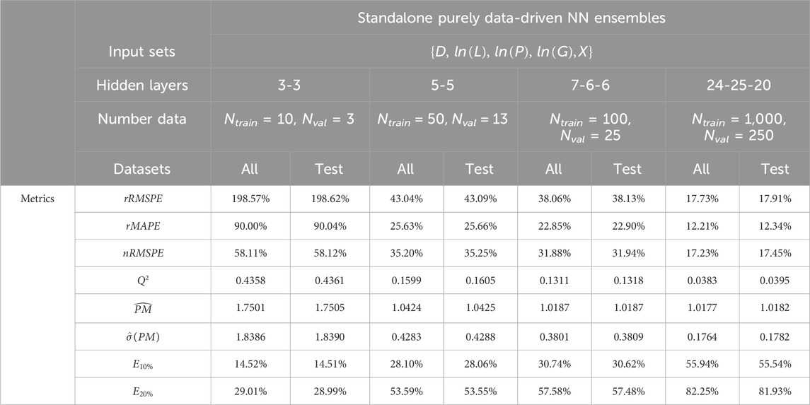
Table 7. Performance metrics (Section 4.4) obtained by purely data-driven NN ensembles (B = 100, S = 20) with inputs $\left\{D,\mathit{ln}\left(L\right),\mathit{ln}\left(P\right),\mathit{ln}\left(G\right),X\right\}$, using small training sets of different sizes, i.e., N_train = 10, 50, 100 and 1,000.

Table 8

Table 8. Performance metrics (Section 4.4) obtained by Res-PENN ensembles (B = 100, S = 20) relying on the empirical Groeneveld LUT and the improved Liu as domain knowledge- and mechanistic physics-based reference models, with inputs $\left\{D,\mathit{ln}\left(L\right),\mathit{ln}\left(P\right),\mathit{ln}\left(G\right),X\right\}$ and using small training sets of different sizes, i.e., N_train = 10, 50, 100 and 1,000.

Table 9

Table 9. Performance metrics (Section 4.4) obtained by HLF-PENN ensembles (B = 100, S = 20) relying on the empirical Groeneveld LUT and the improved Liu as domain knowledge- and mechanistic physics-based reference models, with inputs $\left\{D,\mathit{ln}\left(L\right),\mathit{ln}\left(P\right),\mathit{ln}\left(G\right),X\right\}$, using small training sets of different sizes (i.e., N_train = 10, 50, 100 and 1,000) and optimal $\mathit{\lambda }$ values.

The results of Table 7 serve as reference comparison for the PENN architectures trained with the same amount of data. Table 8 reports the metrics (Section 4.4) obtained by Res-PENN ensembles relying on the empirical Groeneveld LUT and the improved Liu as domain knowledge- and mechanistic physics-based reference models, using small training sets of different sizes, i.e., N_train = 10, 50, 100 and 1,000. As before, the results are very interesting, since both Res-PENN ensembles significantly improve the performance obtained by the corresponding purely data-driven NN model using the same inputs (Table 7). For example, the corresponding percentage improvements obtained by the LUT-based Res-PENN range from 0.92% ($\widehat{PM}$, N_train = 1,000) to 132.9% ($E_{10\%}$, N_train = 10), with relative reductions in rRMSPE, rMAPE and Q² ranging within 10.3%–66.5%, 20.0%–63.9% and 58.7%–77.7%, respectively, over N_train = 10, 50, 100 and 1,000. Considering the Liu-based Res-PENN, percentage improvements range from 2.1% ($\widehat{PM}$, N_train = 1,000) to 135.6% ($E_{10\%}$, N_train = 100), with relative improvements in rRMSPE, rMAPE, Q², $\widehat{\sigma }\left(PM\right)$ and $E_{20\%}$ ranging within 58.7%–86.5%, 53.5%–77.1%, 54.5%–75.1%, 58.5%–86.8% and 19.1%–97.2%, respectively, over N_train = 10, 50, 100 and 1,000. Some important considerations are in order. In this case, the Liu-based Res-PENN significantly outperforms the LUT-based one for (almost) all the metrics and for all the training set sizes. This confirms that the NN tends to have a more relevant action in situations where residuals are more scattered or biased, i.e., when the reference (knowledge- or physics-based) model presents lower accuracy and precision (in this case, the improved Liu). Also, the superior performance is more evident for very small-sized training and validation sets, i.e., N_train = 10–100, where the percentage improvements reach 135%. Finally, it is impressive that the Liu-based Res-PENN ensemble trained with N_train = 100 and 1,000 data performs comparably and much better, respectively, than a purely data-driven NN ensemble with the same inputs $\left\{D,\mathit{ln}\left(L\right),\mathit{ln}\left(P\right),\mathit{ln}\left(G\right),X\right\}$ and trained on N_train = 17,205 instances (Table 5). These results represent a powerful demonstration of the usefulness of PENNs (in this case, the Liu-based Res-PENN) in the presence of very scarce data, independently of the quality of the reference model.

The HLF-PENN requires the identification of an optimal value for parameter $\lambda$. Figures 5, 6 show the sensitivity of rRMSPE, rMAPE and Q² to λ for the HLF-PENN ensembles, relying on the empirical Groeneveld LUT and the improved Liu as reference models, respectively, with N_train = 10 (A, top-left), 50 (B, top-right), 100 (C, bottom-left) and 1,000 (D, bottom-right). First, it is worth noting that for both the LUT- and Liu-based HLF-PENNs with N_train = 1,000 [Figures 5 and 6 (bottom-right)] a similar behavior is observed with respect to the one of an HLF-PENN trained on N_train = 17,205 patterns (Figure 4). The three error metrics here considered increase when λ goes from 0.0 to 1.0 and no optimization needs to be carried out: thus, the best value of $\lambda$ is 0.0, i.e., a pure data-driven NN model. This is explained again by the fact that the performance of both the LUT and Liu models (Table 4, $\lambda$ = 1.0) is still worse than that of a pure NN constructed using N_build = N_train + N_val = 1,250 data points (Table 7, $\lambda$ = 0.0). Thus, since the hybrid loss function (3) is a mathematical average of these two “extreme” configurations, the HLF-PENN with 0.0 < $\lambda$ < 1.0 is expected to showcase intermediate performances. These results suggest again that different from Res-PENN frameworks, even in the presence of a moderate-sized dataset (e.g., N_build = N_train + N_val = 1,250), in this case the HLF-PENN does not represent a viable option: this is even more true, if the “driving” (data- or physics-based) reference model (Table 4) presents poor predictive capabilities. The behavior is instead different for very small-sized datasets, i.e., N_train = 10, 50 and 100. Focusing on the LUT-based HLF-PENN (Figure 5), it is extremely important to note that even “injecting” a very small amount of background knowledge in the training process (i.e., $\lambda$ = 0.1) can produce a sharp decrease in the three error metrics: for example, reductions of around 80.0%, 77.8% and 87.1% are obtained for rRMSPE, rMAPE and Q², respectively, with N_train = 10. The optimal values of parameter $\lambda$ for the different training set sizes (N_train = 10, 50 and 100) are selected by identifying proper trade-offs based on the evolution of all three metrics with respect to $\lambda$. In particular, the following “empirical” procedure is implemented: (1) each metric is normalized (rRMSPE_norm, rMAPE_norm and $Q_{norm}^2$) in the range [0, 1] with respect to its maximum and minimum values; (2) the corresponding (homogeneous) normalized values are combined in a single “objective function” by a simple (possibly weighed) sum, i.e., $w_{rRMSPE}·{rRMSPE}_{norm}+w_{rMAPE}·{rMAPE}_{norm}+w_{Q_{norm}^2}·Q_{norm}^2$, where the w’s are importance weights arbitrarily assigned by the analyst to each metric. In this paper, $w_{rRMSPE}=w_{rMAPE}=w_{Q_{norm}^2}=1$ for simplicity; (3) identify the (optimal) value of $\lambda$ that minimizes the combined (error metric-based) objective function. Obviously, a more complete homogeneous objective function combining all the performance metrics described in Section 4.4 could be considered: this is left for future research. The optimal $\lambda$ values identified for the LUT-based HLF-PENN are $\lambda$ = 0.4 (N_train = 10), $\lambda$ = 0.3 (N_train = 50) and $\lambda$ = 0.2 (N_train = 100).

Figure 5

Figure 5. Sensitivity of the performance metrics rRMSPE, rMAPE and Q² (Section 4.4) to parameter $\mathit{\lambda }$ = 0, 0.1, … , 0.9, 1, for HLF-PENN ensembles based on the LUT model, with input set $\left\{D,\mathit{ln}\left(L\right),\mathit{ln}\left(P\right),\mathit{ln}\left(G\right),X\right\}$, using small datasets of different sizes: (A) N_train = 10, N_val = 3 (top, left); (B) N_train = 50, N_val = 13 (top, right); (C) N_train = 100, N_val = 25 (bottom, left); (D) N_train = 1,000, N_val = 250 (bottom, right).

Figure 6

Figure 6. Sensitivity of the performance metrics rRMSPE, rMAPE and Q² (Section 4.4) to parameter $\mathit{\lambda }$ = 0, 0.1, … , 0.9, 1, for HLF-PENN ensembles based on the improved Liu model, with inputs $\left\{D,\mathit{ln}\left(L\right),\mathit{ln}\left(P\right),\mathit{ln}\left(G\right),X\right\}$, using small datasets of different sizes: (A) N_train = 10, N_val = 3 (top, left); (B) N_train = 50, N_val = 13 (top, right); (C) N_train = 100, N_val = 25 (bottom, left); (D) N_train = 1,000, N_val = 250 (bottom, right).

The behavior of the Liu-based HLF-PENN presents both similarities and interesting differences with respect to the LUT-based one. On one hand, the introduction of a “small amount” of physics ($\lambda$ = 0.1–0.2) into the PENN construction process is in general sufficient for producing an appreciable decrease in most error metrics: for example, the rRMSPE and rMAPE are reduced by around 21%–85% with respect to a purely data-driven NN model build with the same dataset. On the other hand, the evolution of metric Q² is radically different for the different sizes of the training set. For N_train = 10 it decreases sharply as $\lambda$ moves form 0.0 (Q² ≈ 0.44) to 0.1, where it reaches its minimum value (Q² ≈ 0.26). Instead, for N_train = 50 and 100, Q² increases from around 0.16 and 0.13 ($\lambda$ = 0.0), respectively, to around 0.28 ($\lambda$ = 1.0, i.e., standalone physics-based Liu model). This is because the mechanistic Liu model performs very poorly with respect to Q² (Table 4), and a purely data-driven NN can outperform it even using very scarce data (i.e., N_train = 50 and 100). The conflicting behavior of rRMSPE, rMAPE and Q² with respect to $\lambda$ makes the optimization process (based on the normalized objective function combining the three metrics) mandatory. The optimal $\lambda$ values identified for the Liu-based HLF-PENN are $\lambda$ = 0.1 (N_train = 10), $\lambda$ = 0.95 (N_train = 50) and $\lambda$ = 0.1 (N_train = 100).

Table 9 reports the metrics (Section 4.4) obtained by HLF-PENN ensembles relying on the empirical Groeneveld LUT and the improved Liu as domain knowledge- and mechanistic physics-based reference models, using very small training sets of different sizes, i.e., N_train = 10, 50 and 100, and the optimal values of $\lambda$ identified. The results are very interesting, since both HLF-PENN ensembles improve the performance obtained by the corresponding purely data-driven NN model using the same inputs (Table 7). For example, the corresponding percentage improvements obtained by the LUT-based HLF-PENN range from 1.46% ($\widehat{PM}$, N_train = 100) to 199.8% ($E_{10\%}$, N_train = 10), with relative reductions in rRMSPE, rMAPE, Q² and $\widehat{\sigma }\left(PM\right)$ ranging within 13.2%–82.8%, 15.6%–78.6%, 54.7%–86.7% and 13.4%–81.4%, respectively, over N_train = 10, 50, 100. Considering the Liu-based HLF-PENN, percentage improvements range from 5.0% ($\widehat{PM}$, N_train = 100) to 84.5% ($rRMSPE$, N_train = 10), with relative improvements in rMAPE, Q², $\widehat{\sigma }\left(PM\right)$, $E_{10\%}$ and $E_{20\%}$ ranging within 7.8%–73.0% (N_train = 10–50), 39.0%–40.0% (N_train = 10), 23.8%–83.3% (N_train = 10–100), 70.2%–70.4% (N_train = 10) and 62.1%–62.2% (N_train = 10), respectively. Some important considerations are in order. Different from what has been shown for the Res-PENN approaches (Table 8), the Liu-based HLF-PENN performs comparably to (or better than) the LUT-based one only for N_train = 10, while in all the other cases (N_train = 50–100) it generally underperforms: actually, it presents several metrics (in particular, those related to the model predictive capability and dispersion) that are even worse than those of a purely data-driven NN. For example, a percentage worsening in Q², $E_{10\%}$ and $E_{20\%}$ is observed to range within 74.0%–120.9%, 10.6%–14.7% and 9.5%–14.8%, respectively, over N_train = 50–100. This behavior can be easily explained by the radically different concepts underlying the two PENN frameworks. In the Res-PENN approaches, the worse is the knowledge- or physics-based reference model, the easier is for the NN to capture the corresponding (large) residuals and “absorb” the associated (large) model errors; instead, the performance of HLF-PENN is directly driven by the quality of the reference model included in the NN loss function [formula (3) of Section 4.2.2]. Thus, more biased, less accurate and more dispersed models (like the Liu model in this case) will lead to worse physics-informed predictions. Finally, from the comparison of Table 8 and Table 9, the following relevant conclusions can be drawn: (i) for relatively small- and moderate-sized datasets (N_train = 100–1,000) the Res-PENN approaches show here consistently better results, in particular when combined with the improved Liu model; (ii) for very small-sized datasets (N_train = 10–50) it becomes difficult also for the Res-PENN to capture the undiscovered trends and absorb the systematic model errors: thus, the HLF-PENN starts to play an interesting role (in particular, when hybridized with the empirical LUT model).

6.3 Uncertainty in the PENN predictions of the CHF

The uncertainty in CHF predictions (resulting from the finiteness of the training datasets, the randomness in the training process and model architecture) is quantified by 95% Prediction Intervals (PIs) $\left[{\underset{\_}{q}}_i^{CHF,95\%},{\overline{q}}_i^{CHF,95\%}\right]$ by the original (nested) combination of the bootstrap method (B = 100) and the randomized weight/bias initialization strategy (S = 20) presented in Section 4.3. The results are presented in terms of Coverage Probability (CP) and Normalized Mean Width (NMW) in Figure 7 for all the purely-data driven NN- and PENN-based models described in this work with inputs $\left\{D,\mathit{ln}\left(L\right),\mathit{ln}\left(P\right),\mathit{ln}\left(G\right),X\right\}$; however, among them, also the pure data-driven NN with inputs $\left\{D,\mathit{ln}\left(L\right),\mathit{ln}\left(P\right),\mathit{ln}\left(G\right),\Delta h_{in}\right\}$ and N_train = 17,205 is included as the best reference case (circle, CP = 95.15%, NMW = 0.0079). In general, the larger the CP and the smaller the NMW (top-left corner of the figures), the better the prediction model; also, notice that for 95% PIs, if the empirical CP is smaller than 95%, in principle the corresponding model should not be considered as statistically validated. Four of the configurations analyzed result not validated: the purely data-driven NNs trained by small- and moderate-sized datasets, i.e., N_train = 50 (triangle-up), 100 (diamond) and 1,000 (square), and the (LUT- and Liu-based) Res-PENN built with very scarce data, i.e., N_train = 10 (triangle-down); however, two of them fail by a small amount, showing a CP of around 94%. Paradoxically, the (inaccurate) data-driven NN with N_train = 10 (horizontal line) turns out to be validated (CP = 98.56%) thanks to the very high uncertainty associated with the CHF estimates, i.e., NMW = 0.6111. Instead, besides the NN including inlet subcooling ($\Delta h_{in}$) as input, the best performing models are the data-driven NN (plus) and the (LUT- and Liu-based) Res-PENN (asterisk) trained with the entire USNRC dataset, and the Liu-based Res-PENN using N_train = 1,000 patterns (Figure 7, right), x-mark), showing CPs and NMWs within 95.10%–95.40% and 0.0108–0.0309, respectively.

Figure 7

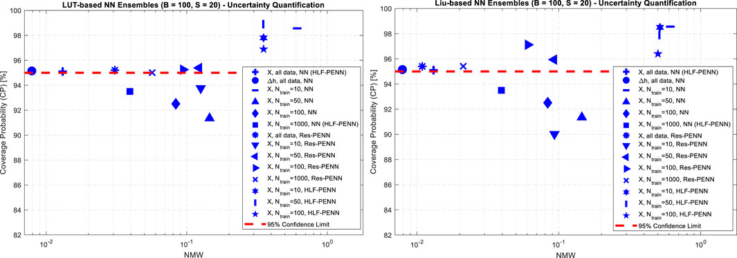
Figure 7. Coverage Probability (CP) and Normalized Mean Width (NMW) for the 95% Prediction Intervals (PIs) of the CHF predictions produced by all the NN- and PENN-based approaches here considered: (A) empirical LUT-based models (left); (B) mechanistic physics-based improved Liu model (right).

The uncertainty analyses of the PENN frameworks confirm to some extent the findings highlighted in the previous sections. When the Res-PENN approaches are adopted (asterisk, triangle-down, triangle-left, triangle-right, x-mark in Figure 7), the combination with the (worse performing) mechanistic physics-based Liu model produces more appreciable (i.e., less uncertain) results than the LUT: among the validated models, the corresponding NMWs (resp., the PIs) are 1.32–2.83 times smaller (resp., tighter). Instead, when the HLF-PENNs are embraced (hexagram, vertical line, pentagram in Figure 7), the best performances are obtained by hybridization with the (best performing) empirical LUT model: actually, the corresponding NMWs (resp., the PIs) are 1.42–1.47 times smaller (resp., tighter).

Finally, from the comparison of the general performance of classical NN, Res-PENN and HLF-PENN frameworks, it can be seen that: (i) for small- (N_train = 50–100) and moderate-sized (N_train = 1,000) datasets, PENNs are evidently preferable than classical NNs, as the CPs of their 95% PIs sre consistently larger than 95%, while most of the purely data-driven NN models are not validated; (ii) Res-PENN algorithms represent in general more convenient options than HLF-PENN ones, as their CHF estimates are much more precise (i.e., less uncertain): the corresponding NMWs are 3.0–24.5 times smaller; (iii) the HLF-PENN framework becomes an interesting option when the training set size is very small (N_train = 10–50), as it can produce validated models (differently from the other approaches); on the other hand, the associated uncertainty is typically overestimated, as it can be argued by the “excessive” values of the CPs (96.4%–98.9%, i.e., much larger than 95%) and by the comparatively large PIs (i.e., NMWs around 0.50–0.52).

7 Conclusion

In this paper, Residual- and Hybrid Loss Function-based Physics Enhanced Neural Networks (Res- and HLF-PENNs, respectively) using 5 input variables (pressure, hydraulic diameter, mass flux, heated length and critical quality) have been thoroughly and systematically compared in the tasks of accurately and precisely predicting the Critical Heat Flux (CHF) in nuclear reactors and of estimating the corresponding uncertainty. Two reference (prior) models have been considered for hybridization with NNs to produce PENN frameworks: the empirical (data-driven) Groeneveld Look-Up Table (LUT) (Groeneveld, 2019) and an improved version of the mechanistic physics-based Liu model (Liu et al., 2012). The main methodological and applicative contributions of the work can be summarized as follows:

⁃ While the HLF-PENN methodology has proven beneficial across a variety of physics domains, few or no applications to CHF prediction in nuclear reactors are available in the open literature up to now;

⁃ the improved Liu model proposed in Liu et al. (2012) has been considered for the first time within a PENN-based CHF prediction framework, as it covers a much wider range of thermodynamic conditions (i.e., both subcooled and saturated boiling) with respect to the original one (Liu et al., 2000; Zhao et al., 2020);

⁃ it was the first time that the Res-PENN and HLF-PENN approaches have been systematically compared, with particular reference to the task of estimating CHF in the presence of very scarce data (i.e., a few tens or hundreds training patterns), which is of paramount importance in the nuclear industry, where collecting a large amount of high-quality data is often too costly (and sometimes even impossible);

⁃ the uncertainty in the PENN predictions (due to the finiteness of the training dataset, randomness in the training process and model architecture) has been quantified by an ensemble-based approach, conceived as an original combination of two nested procedures involving the bootstrap method and a random weight/bias initialization strategy.

The application of the methods to the United States Nuclear Regulatory Commission (USNRC) CHF dataset from (Groeneveld, 2019) has allowed to derive the following guidelines and conclusions:

⁃ When very large datasets (i.e., containing >> 1,000 training patterns) are available:

o Classical, purely data-driven NNs can obtain excellent performances (e.g., rMAPE ≈ 2.58–7.73%) that are consistently superior to those of the standalone reference LUT and improved Liu models. More important, the results are at least comparable to (or even better than) those reported in the open literature and produced by more sophisticated algorithms (e.g., Convolutional Neural Networks-CNNs, Transformers, Ensembles of Deep Sparse AutoEncoders, …) employing a higher number of inputs and/or more complex structures and architectures (i.e., a much larger number of adjustable parameters);

o The very flexible Res-PENN framework can significantly improve the results obtained by purely data-driven NN models, showing performances that are almost independent of the embedded knowledge-based reference model (i.e., either LUT or Liu). Thanks to the availability of large data, the Res-PENN is very efficient in capturing and “absorbing” the associated model errors and biases, no matter the quality of the prior model;

o The HLF-PENN does not seem to represent the most convenient option, in particular when the (data- or physics-based) prior reference models “driving” the NN hybrid loss function are imperfect and show comparatively poor predictive capabilities with respect to purely data-driven ones (like in the present case), However, this conclusion (which seems to “limit” the effectiveness of HLF-PENNs in the presence of large data) has not been formally and analytically proven by the author, it may depend to some extent on the particular engineering problem at hand and, above all, on the particular task requested to the ML algorithm (i.e, , regression and/or interpolation and/or extrapolation), Thus, even in the presence of large datasets, quick testing and optimization of the weighting hyperparameter $\lambda$ is still suggested to practitioners, as a preliminary, fast check on the HLF-PENN performances

⁃ When moderate-sized datasets (i.e., containing ≈1,000 training patterns) are available, the use of Res-PENN ensembles is strongly suggested, as they significantly improve the performance of purely data-driven NN models. However, as the number of data points decreases, the Res-PENN is shown to have an increasingly powerful action in situations where residuals/errors are more scattered or biased, i.e., when the reference (knowledge- or physics-based) model presents lower accuracy and precision (in this case, the improved Liu). Thus, a combination/hybridization with a poorly performing reference model is (paradoxically) preferable, as also found by Zhao et al. (2020).

⁃ Instead, when very small-sized datasets (i.e., containing ≈10–100 training patterns) are available, it becomes difficult even for the Res-PENN to capture effectively the undiscovered trends and absorb systematic model errors. Thus, the HLF-PENN framework starts to play an interesting role and may be taken as the preferable option, provided that: i) the weighting parameter $\lambda$ in the hybrid NN loss function is accurately optimized with respect to all the performance metrics of interest; ii) satisfactory physical models/correlations or even mechanistic models representing the “ground truth” for a given phenomenon are available for effectively “driving” the NN training.

With respect to the quantification of uncertainty, it can be concluded that:

⁃ for small- (50–100 points) and moderate-sized (1,000 points) datasets, PENNs are evidently preferable than classical purely data-driven NNs, whose models are typically not validated from a statistical viewpoint;

⁃ Res-PENN algorithms represent in this case more convenient options than HLF-PENN ones, as their CHF estimates are much more precise (i.e., less uncertain);

⁃ the HLF-PENN framework becomes an interesting option only when the training set size is very small (10–50 points), as it can produce validated models (differently from the other approaches). On the other hand, their associated uncertainty is typically overestimated, as can be argued by the comparatively large width of the Prediction Intervals.

Future research will be devoted to: (i) testing the proposed PENN models on different datasets and possibly on different tube geometries; (ii) testing the PENNs extrapolation capabilities (i.e., predictions outside the training ranges): in this condition, HLF-PENNs are expected to play a relevant role, thanks to the presence of a reference prior model, which “emerges” in the hybrid loss function and compensates for the complete lack of experimental (training) data in the extrapolation range; (iii) creating Res-PENN and HLF-PENN algorithms based on the hybridization with new (possibly more accurate, more precise and less biased) empirical correlations and/or mechanistic physics-based models (when available, rigorous first-principle physical laws representing the “ground truth” for the phenomena of interest could be implemented): ideally, an ensemble of reference (prior) models could be considered, each one showing outstanding performances over a limited portion of the input space; (iv) comparing the ensemble-based strategy for uncertainty quantification with other approaches, e.g., dropout Neural Networks, Bayesian Neural Networks or In-series Neural Networks (Tran et al., 2020; Furlong et al., 2025a); (v) testing the PENN models on the “slice” datasets provided by the leaders of the “Task Force on Artificial Intelligence and Machine Learning for Scientific Computing in Nuclear Engineering” (i.e., datasets where only one input parameter at a time is allowed to vary within predefined intervals, while all the other parameters are kept reasonably constant). The objective is twofold: (a) although overfitting has been here carefully avoided by early stopping and accurate selection of the NN architecture and number of adjustable hyperparameters, this analysis will help demonstrating further the PENNs predictive and generalization capabilities; (b) visualizing how the uncertainty unfolds over the “slice” datasets will help checking if and how the PIs change expectedly in regions of data sparsity with respect to those of high data density.

Data availability statement

The original contributions presented in the study are included in the article/supplementary material, further inquiries can be directed to the corresponding author.

Author contributions

NP: Writing – original draft, Software, Resources, Visualization, Methodology, Formal Analysis, Conceptualization, Validation, Data curation, Writing – review and editing, Investigation.

Funding

The authors declare that no financial support was received for the research and/or publication of this article.

Acknowledgements

The author would like to acknowledge the contribution of all those individuals who had a key role and leadership in the conduct of the activity of the OECD/NEA/WPRS/EGMUP “Task Force on Artificial Intelligence and Machine Learning for Scientific Computing in Nuclear Engineering”, especially the task leaders: Jean-Marie LE CORRE (Westinghouse Electric Sweden AB, Sweden), Gregory DELIPEI (North Carolina State University, United States), Xu WU (North Carolina State University, United States), Xingang ZHAO (Oak Ridge National Laboratory, United States), Oliver BUSS (NEA).

Conflict of interest

The author declares that the research was conducted in the absence of any commercial or financial relationships that could be construed as a potential conflict of interest.

The author(s) declared that they were an editorial board member of Frontiers, at the time of submission. This had no impact on the peer review process and the final decision.

Generative AI statement

The authors declare that no Generative AI was used in the creation of this manuscript.

Any alternative text (alt text) provided alongside figures in this article has been generated by Frontiers with the support of artificial intelligence and reasonable efforts have been made to ensure accuracy, including review by the authors wherever possible. If you identify any issues, please contact us.

Publisher’s note

All claims expressed in this article are solely those of the authors and do not necessarily represent those of their affiliated organizations, or those of the publisher, the editors and the reviewers. Any product that may be evaluated in this article, or claim that may be made by its manufacturer, is not guaranteed or endorsed by the publisher.

References

Abrate, N., Dulla, S., and Pedroni, N. (2023a). A non-intrusive reduced order model for the characterisation of the spatial power distribution in large thermal reactors. Ann. Nucl. Energy 184, 109674–4549. doi:10.1016/j.anucene.2022.109674

CrossRef Full Text | Google Scholar

Abrate, N., Moscatello, A., Ledda, G., Pedroni, N., Carbone, F., Maffia, E., et al. (2023b). A novel approach combining bootstrapped non-intrusive reduced order models and unscented transform for the robust and efficient CFD analysis of accidental gas releases in congested plants. J. Loss Prev. Process Industr. 83, 105015–4230. doi:10.1016/j.jlp.2023.105015

CrossRef Full Text | Google Scholar

Acuña, G., Cubillos, F., Thibault, J., and Latrille, E. (1999). Comparison of methods for training grey-box neural network models. Comput. Chem. Eng. 23, S561–S564. doi:10.1016/S0098-1354(99)80138-0

CrossRef Full Text | Google Scholar

Ahmed, I., Gatti, I., and Zio, E. (2025). “Prediction of critical heat flux in vertical tubes by physics-informed neural networks,” in Proceedings of the 35th European safety and reliability and the 33rd society for risk analysis Europe conference 2025 ESREL SRA-E 2025 Organizers. Editors E. Bjorheim Abrahamsen, T. Aven, F. Bouder, R. Flage, and M. Ylönen (Singapore: Research Publishing), 2601–2608. doi:10.3850/978-981-94-3281-3_ESREL-SRA-E2025-P3221-cd

CrossRef Full Text | Google Scholar

Ak, R., Li, Y. F., Vitelli, V., Zio, E., Droguett, E. L., and Jacinto, C. M. C. (2013). NSGA-II-trained neural network approach to the estimation of prediction intervals of scale deposition rate in oil & gas equipment. Expert Syst. Appl. 40 (4), 1205–1212. doi:10.1016/j.eswa.2012.08.018

CrossRef Full Text | Google Scholar

Alsafadi, F., Furlong, A., and Wu, X. (2025). Predicting critical heat flux with uncertainty quantification and domain generalization using conditional variational autoencoders and deep neural networks. Ann. Nucl. Energy 220 (15 September 2025), 111502. doi:10.1016/j.anucene.2025.111502

CrossRef Full Text | Google Scholar

Antonello, F., Buongiorno, J., and Zio, E. (2023). Physics informed neural networks for surrogate modeling of accidental scenarios in nuclear power plants. Nucl. Eng. Technol. 55, 3409–3416. doi:10.1016/j.net.2023.06.027

CrossRef Full Text | Google Scholar

Biasi, L., Clerici, G. C., Garribba, S., Sala, R., and Tozzi, A. (1967). Studies on burnout. Part 3: a new correlation for round ducts and uniform heating and its comparison with world data. Energ. Nuclare 14, 530–536.

Google Scholar

Bowring, R. A. (1972). Simple but accurate round tube, uniform heat flux, dryout correlation over the pressure range 0.7–17 MN/m₂ (100–2500 PSIA). Oxfordshire, UK: PSIA UKAEA Reactor Group, 100–2500.

Google Scholar

Bruder, M., Bloch, G., and Sattelmayer, T. (2017). Critical heat flux in flow boiling - review of the current understanding and experimental approaches. Heat. Transf. Eng. 38, 347–360. doi:10.1080/01457632.2016.1189274

CrossRef Full Text | Google Scholar

Bucci, M. (2017). “Advanced diagnostics to resolve long-lasting controversies in boiling heat transfer,” in Proceedings of the 13th international conference on heat transfer, fluid mechanics and thermodynamics (Portoroz, Slovenia: HEFAT), 324–327.

Google Scholar

Cabarcos, A., Paz, C., Suarez, E., and Vence, J. (2024). Application of supervised learning algorithms for temperature prediction in nucleate flow boiling. Appl. Therm. Eng. 240, 122155. doi:10.1016/j.applthermaleng.2023.122155

CrossRef Full Text | Google Scholar

Cai, S., Wang, Z., Wang, S., Perdikaris, P., and Karniadakis, G. E. (2021). Physics-informed neural networks for heat transfer problems. J. Heat Transf. 143 (6), 060801. doi:10.1115/1.4050542

CrossRef Full Text | Google Scholar

Castrignanò, D. (2025). Development of artificial neural network (ANN) models for critical heat flux predictions. Torino, Italy: Supervisor: Prof. Nicola Pedroni. Politecnico di Torino. Thesis for the obtainment of the MSc Degree in Energy and Nuclear Engineering. Available online at: https://webthesis.biblio.polito.it/34961/.

Google Scholar

Celata, G. P., Cumo, M., Mariani, A., Simoncini, M., and Zummo, G. (1994). Rationalization of existing mechanistic models for the prediction of water subcooled flow boiling critical heat flux. Int. J. Heat. Mass Transf. 37, 347–360. doi:10.1016/0017-9310(94)90035-3

CrossRef Full Text | Google Scholar

Celata, G. P., Cumo, M., Katto, Y., and Mariani, A. (1999). Prediction of the critical heat flux in water subcooled flow boiling using a new mechanistic approach. Int. J. Heat. Mass Transf. 42, 1457–1466. doi:10.1016/S0017-9310(98)00286-5

CrossRef Full Text | Google Scholar

Chicco, D. (2017). Ten quick tips for machine learning in computational biology. BioData Min. 10 (35), 35–17. doi:10.1186/s13040-017-0155-3

PubMed Abstract | CrossRef Full Text | Google Scholar

Cicirello, A. (2024). Physics-enhanced machine learning: a position paper for dynamical systems investigations. J. Phys. Conf. Ser. 2909, 012034. doi:10.1088/1742-6596/2909/1/012034

CrossRef Full Text | Google Scholar

Cuomo, S., Di Cola, V. S., Giampaolo, F., Rozza, G., Raissi, M., and Piccialli, F. (2022). Scientific machine learning through physics–informed neural networks: where we are and what’s next. J. Sci. Comput. 92, 88. doi:10.1007/s10915-022-01939-z

CrossRef Full Text | Google Scholar

Cybenko, G. (1989). Approximation by superpositions of a sigmoidal function. Math. Control Signals Syst. 2, 303–314. doi:10.1007/bf02551274

CrossRef Full Text | Google Scholar

De la Mata, F. F., Gijón, A., Molina-Solana, M., and Gómez-Romero, J. (2023). Physics-informed neural networks for data-driven simulation: advantages, limitations, and opportunities. Phys. A Stat. Mech. its Appl. 610, 128415. doi:10.1016/j.physa.2022.128415

CrossRef Full Text | Google Scholar

Diao, Y., Yang, J., Zhang, Y., Zhang, D., and Du, Y. (2023). Solving multi-material problems in solid mechanics using physics-informed neural networks based on domain decomposition technology. Comput. Methods Appl. Mech. Eng. 413, 116120. doi:10.1016/j.cma.2023.116120

CrossRef Full Text | Google Scholar

Efron, B., and Tibshirani, R. J. (1994). An introduction to the bootstrap. 1st ed. New York, NY: Chapman and Hall/CRC. doi:10.1201/9780429246593

CrossRef Full Text | Google Scholar

Farea, A., Yli-Harja, O., and Emmert-Streib, F. (2024). Understanding physics-informed neural networks: techniques, applications, trends, and challenges. AI 5, 1534–1557. doi:10.3390/ai5030074

CrossRef Full Text | Google Scholar

Ferrario, E., Pedroni, N., Zio, E., and Lopez-Caballero, F. (2017). Bootstrapped artificial neural networks for the seismic analysis of structural systems. Struct. Saf. 67, 70–84. doi:10.1016/j.strusafe.2017.03.003

CrossRef Full Text | Google Scholar

Forssell, U., and Lindskog, P. (1997). Combining semi-physical and neural network modeling: an example of its usefulness. IFAC Proc. 30, 767–770. doi:10.1016/S1474-6670(17)42938-7

CrossRef Full Text | Google Scholar

Furlong, A., Zhao, X., Salko, R. K., and Wu, X. (2025a). Physics-based hybrid machine learning for critical heat flux prediction with uncertainty quantification. Appl. Therm. Eng. 279, 127447. doi:10.1016/j.applthermaleng.2025.127447

CrossRef Full Text | Google Scholar

Furlong, A., Zhao, X., Salko, R. K., and Wu, X. (2025b). Deployment of traditional and hybrid machine learning for critical heat flux prediction in the CTF thermal hydraulics code. arXiv:2505. doi:10.48550/arXiv.2505.14701

CrossRef Full Text | Google Scholar

Groeneveld, D. (2019). Critical heat flux data used to generate the 2006 groeneveld lookup tables. Tech. Rep. Washington, DC: United States Nuclear Regulatory Commission.

Google Scholar

Groeneveld, D. C., Leung, L. K. H., Guo, Y., Vasic, A., El Nakla, M., Peng, S. W., et al. (2005). Lookup tables for predicting CHF and film-boiling heat transfer: past, present, and future. Nucl. Technol. 152 (1), 87–104. doi:10.13182/NT152-87

CrossRef Full Text | Google Scholar

Groeneveld, D., Shan, J., Vasic, A., Leung, L., Durmayaz, A., Yang, J., et al. (2007). The 2006 CHF look-up table. Nucl. Eng. Des. 237, 1909–1922. doi:10.1016/j.nucengdes.2007.02.014

CrossRef Full Text | Google Scholar

Groeneveld, D., Ireland, A., Kaizer, J., and Vasic, A. (2018). An overview of measurements, data compilations and prediction methods for the critical heat flux in water-cooled tubes. Nucl. Eng. Des. 331, 211–221. doi:10.1016/j.nucengdes.2018.02.031

CrossRef Full Text | Google Scholar

Grosfilley, E. H. (2022). Investigation of machine learning regression techniques to predict critical heat flux. MSc Dissertation, Uppsala Universitet, UPTEC F, ISSN 1401-5757; 22041. Available online at: https://urn.kb.se/resolve?urn=urn:nbn:se:uu:diva-479159.

Google Scholar

Grosfilley, E. H., Robertson, G., Soibam, J., and Le Corre, J.-M. (2024). Investigation of machine learning regression techniques to predict critical heat flux over a large parameter space. Nucl. Technol. 211 (10), 1–15. doi:10.1080/00295450.2024.2380580

CrossRef Full Text | Google Scholar

Hall, D. D., and Mudawar, I. (2000). Critical heat flux (CHF) for water flow in tubes - II: subcooled CHF correlations. Int. J. Heat Mass Transf. 43, 2605–2640. doi:10.1016/s0017-9310(99)00192-1

CrossRef Full Text | Google Scholar

He, M., and Lee, Y. (2018). Application of machine learning for prediction of critical heat flux: support vector machine for data-driven CHF look-up table construction based on sparingly distributed training data points. Nucl. Eng. Des. 338, 189–198. doi:10.1016/j.nucengdes.2018.08.005

CrossRef Full Text | Google Scholar

He, M., and Lee, Y. (2020). Application of deep belief network for critical heat flux prediction on microstructure surfaces. Nucl. Technol. 206 (2), 358–374. doi:10.1080/00295450.2019.1626177

CrossRef Full Text | Google Scholar

Hedayat, A. (2021). Developing a robust and flexible smart tool to predict a full range critical heat flux (CHF) in different LWRs by using deep learning artificial neural networks (ANN) via parallel multi-processing. Prog. Nucl. Energy 142, 103985. doi:10.1016/j.pnucene.2021.103985

CrossRef Full Text | Google Scholar

Hong, Q., Jun, M., Bo, W., Sichao, T., Jiayi, Z., Biao, L., et al. (2023). Application of data-driven technology in nuclear engineering: prediction, classification and design optimization. Ann. Nucl. Energy 194, 110089. doi:10.1016/j.anucene.2023.110089

CrossRef Full Text | Google Scholar

Huang, Q., Peng, S., Deng, J., Zeng, H., Zhang, Z., Liu, Y., et al. (2023). A review of the application of artificial intelligence to nuclear reactors: where we are and what’s next. Heliyon 9 (3), e13883. doi:10.1016/j.heliyon.2023.e13883

PubMed Abstract | CrossRef Full Text | Google Scholar

Jalili, D., Jang, S., Jadidi, M., Giustini, G., Keshmiri, A., and Mahmoudi, Y. (2024). Physics-informed neural networks for heat transfer prediction in two-phase flows. Int. J. Heat Mass Transf. 221, 125089. doi:10.1016/j.ijheatmasstransfer.2023.125089

CrossRef Full Text | Google Scholar

Jiang, B., Zhou, J., Huang, X., and Wang, P. (2020). Prediction of critical heat flux using gaussian process regression and ant colony optimization. Ann. Nucl. Energy 149, 107765. doi:10.1016/j.anucene.2020.107765

CrossRef Full Text | Google Scholar

Jin, X., Cai, S., Li, H., and Karniadakis, G. E. (2021). NSFnets (Navier-Stokes flow nets): physics-informed neural networks for the incompressible Navier-Stokes equations. J. Comput. Phys. 426, 109951. doi:10.1016/j.jcp.2020.109951

CrossRef Full Text | Google Scholar

Kaminaga, M., Yamamoto, K., and Sudo, Y. (1988). Improvement of critical heat flux correlation for research reactors using plate-type fuel. J. Nucl. Sci. Technol. 35 (12), 943–951. doi:10.1080/18811248.1998.9733966

CrossRef Full Text | Google Scholar

Kandlikar, S. G. (2001). Critical heat flux in subcooled flow boiling—an assessment of current understanding and future directions for research. Multiph. Sci. Technol. 13, 26–130. doi:10.1615/MultScienTechn.v13.i3-4.40

CrossRef Full Text | Google Scholar

Karpatne, A., Atluri, G., Faghmous, J. H., Steinbach, M., Banerjee, A., Ganguly, A., et al. (2017). Theory-guided data science: a new paradigm for scientific discovery from data. IEEE Trans. Knowl. Data Eng. 29 (10), 2318–2331. doi:10.1109/TKDE.2017.2720168

CrossRef Full Text | Google Scholar

Katto, Y. (1978). A generalized correlation of critical heat flux for the forced convection boiling in vertical uniformly heated round tubes. Int. J. Heat. Mass Transf. 21, 1527–1542. doi:10.1016/0017-9310(78)90009-1

CrossRef Full Text | Google Scholar

Katto, Y. (1981). General features of CHF of forced convection boiling in uniformly heated rectangular channels. Int. J. Heat. Mass Transf. 24 (8), 1413–1419. doi:10.1016/0017-9310(80)90091-5

CrossRef Full Text | Google Scholar

Katto, Y. (1990). A physical approach to critical heat flux of subcooled flow boiling in round tubes. Int. J. Heat. Mass Transf. 33, 611–620. doi:10.1016/0017-9310(90)90160-V

CrossRef Full Text | Google Scholar

Katto, Y. (1992). A prediction model of subcooled water flow boiling CHF for pressure in the range 0.1–20 MPa. Int. J. Heat Mass Transf. 35 (5), 1115–1123. doi:10.1016/0017-9310(92)90172-O

CrossRef Full Text | Google Scholar

Khalid, R. Z., Ullah, A., Khan, A., Khan, A., and Inayat, M. H. (2023). Comparison of standalone and hybrid machine learning models for prediction of critical heat flux in vertical tubes. Energies 16 (7), 3182. doi:10.3390/en16073182

CrossRef Full Text | Google Scholar

Khalid, R. Z., Ahmed, I., Ullah, A., Zio, E., and Khan, A. (2024a). Enhancing accuracy of prediction of critical heat flux in circular channels by ensemble of deep sparse autoencoders and deep neural networks. Nucl. Eng. Des. 429, 113587. doi:10.1016/j.nucengdes.2024.113587

CrossRef Full Text | Google Scholar

Khalid, R. Z., Ullah, A., Khan, A., Al-Dahhan, M. H., and Inayat, M. H. (2024b). Dependence of critical heat flux in vertical flow systems on dimensional and dimensionless parameters using machine learning. Int. J. Heat. Mass Tran. 225, 125441. doi:10.1016/j.ijheatmasstransfer.2024.125441

CrossRef Full Text | Google Scholar

Kim, H., Moon, J., Hong, D., Cha, E., and Yun, B. (2021). Prediction of critical heat flux for narrow rectangular channels in a steady state condition using machine learning. Nucl. Eng. Technol. 53 (6), 1796–1809. doi:10.1016/j.net.2020.12.007

CrossRef Full Text | Google Scholar

Kim, K. M., Hurley, P., and Duarte, J. P. (2022a). High-resolution prediction of quenching behavior using machine learning based on optical fiber temperature measurement. Int. J. Heat. Mass Tran. 184, 122338. doi:10.1016/j.ijheatmasstransfer.2021.122338

CrossRef Full Text | Google Scholar

Kim, K. M., Hurley, P., and Duarte, J. P. (2022b). Physics-informed machine learning-aided framework for prediction of minimum film boiling temperature. Int. J. Heat. Mass Tran. 191, 122839. doi:10.1016/j.ijheatmasstransfer.2022.122839

CrossRef Full Text | Google Scholar

Kumar, V., Pimparkar, D., Saini, V. R., Kohli, R., Gupta, S., and Pothukuchi, H. (2024). Prediction of CHF location through applied machine learning. Prog. Nucl. Energy 169, 105055. doi:10.1016/j.pnucene.2024.105055

CrossRef Full Text | Google Scholar

Lai, C., Ahmed, I., Zio, E., Li, W., Zhang, Y., Yao, W., et al. (2024). A multistage physics-informed neural network for fault detection in regulating valves of nuclear power plants. Energies 17, 2647. doi:10.3390/en17112647

CrossRef Full Text | Google Scholar

Le Corre, J.-M., Wu, X., and Zhao, X. (2024). “Benchmark on artificial intelligence and machine learning for scientific computing in nuclear engineering. Phase 1: critical heat flux exercise specifications,” in NEA working papers, NEA/WKP(2023)1. Paris: OECD Publishing.

Google Scholar

LeCun, Y., Bengio, Y., and Hinton, G. (2015). Deep learning. Nature 521 (7553), 436–444. doi:10.1038/nature14539

PubMed Abstract | CrossRef Full Text | Google Scholar

Lee, C. H., and Mudawwar, I. (1988). A mechanistic critical heat flux model for subcooled flow boiling based on local bulk flow conditions. Int. J. Multiph. Flow. 14, 711–728. doi:10.1016/0301-9322(88)90070-5

CrossRef Full Text | Google Scholar

Li, C., Mu, X., Hu, S., and Shen, S. (2024). Comparative analysis of heat transfer prediction for falling film evaporation on the horizontal tube based on machine learning methods. Int. J. Therm. Sci. 203, 109165. doi:10.1016/j.ijthermalsci.2024.109165

CrossRef Full Text | Google Scholar

Liu, W. (2022). Prediction of critical heat flux for subcooled flow boiling in annulus and transient surface temperature change at CHF. Fluids 7 (7), 230. doi:10.3390/fluids7070230

CrossRef Full Text | Google Scholar

Liu, W., Nariai, H., and Inasaka, F. (2000). Prediction of critical heat flux for subcooled flow boiling. Int. J. Heat. Mass Transf. 43, 3371–3390. doi:10.1016/S0017-9310(99)00373-7

CrossRef Full Text | Google Scholar

Liu, W. X., Tian, W. X., Wu, Y. W., Su, G. H., Qiu, S. Z., Yan, X., et al. (2012). An improved mechanistic critical heat flux model and its application to motion conditions. Prog. Nucl. Energy 61, 88–101. doi:10.1016/j.pnucene.2012.07.002

CrossRef Full Text | Google Scholar

Lye, A., Ong, T. K. C., Xiao, S., and Chung, K. Y. (2025). Physics-enhanced machine learning for probabilistic risk assessment in nuclear safety: an overview, recent developments, and perspectives. Ann. Nucl. Energy 222, 111562. doi:10.1016/j.anucene.2025.111562

CrossRef Full Text | Google Scholar

Mao, C., and Jin, Y. (2024). Uncertainty quantification study of the physics-informed machine learning models for critical heat flux prediction. Prog. Nucl. Energy 170, 105097. doi:10.1016/j.pnucene.2024.105097

CrossRef Full Text | Google Scholar

Marino, L., and Cicirello, A. (2023). A switching Gaussian process latent force model for the identification of mechanical systems with a discontinuous nonlinearity. Data-Centric Eng. 4, e18. doi:10.1017/dce.2023.12

CrossRef Full Text | Google Scholar

Mirshak, S., Durant, W. S., and Towell, R. H., (1959). Heat flux at Burnout. Aiken, SC: E.I. du Pont de Nemours & Co., Explosives Dept., Atomic Energy Division, Technical Division, Savannah River Laboratory, 16.

Google Scholar

Mudawar, I., Darges, S. J., and Devahdhanush, V. S. (2024). Prediction technique for flow boiling heat transfer and critical heat flux in both microgravity and Earth gravity via artificial neural networks (ANNs). Int. J. Heat Mass Transf. 220, 124998. doi:10.1016/j.ijheatmasstransfer.2023.124998

CrossRef Full Text | Google Scholar

Nassif, A. B., Shahin, I., Attili, I., Azzeh, M., and Shaalan, K. (2019). Speech recognition using deep neural networks: a systematic review. IEEE Access 7, 19143–19165. doi:10.1109/ACCESS.2019.2896880

CrossRef Full Text | Google Scholar

Niu, S., Bi, J., Li, Y., and Lu, G. (2024). Prediction of critical heat flux and position in narrow rectangular channels using deep feed-forward neural networks coupling with empirical correlations. Int. J. Heat Mass Transf. 221, 125042. doi:10.1016/j.ijheatmasstransfer.2023.125042

CrossRef Full Text | Google Scholar

Noh, H., Kim, K., and Nahm, K. (2014). “Assessment of the water CHF Look-up table for rod bundles CHF measurements,” in Proceedings of the KNS 2014 spring meeting. 28–30 May 2014, Jeju, Korea, KNS, 3.

Google Scholar

Okawa, T., Kotani, A., Kataoka, I., and Naitoh, M. (2004). Prediction of the critical heat flux in annular regime in various vertical channels. Nucl. Eng. Des. 229, 223–236. doi:10.1016/j.nucengdes.2004.01.005

CrossRef Full Text | Google Scholar

Park, H. M., Lee, J. H., and Kim, K. D. (2020). Wall temperature prediction at critical heat flux using a machine learning model. Ann. Nucl. Energy 141, 107334. doi:10.1016/j.anucene.2020.107334

CrossRef Full Text | Google Scholar

Pedroni (2022). “Computational methods for the robust optimization of the design of a dynamic aerospace system in the presence of aleatory and epistemic uncertainties,” in Mechanical systems and signal processing (special issue NASA langley challenge on optimization under uncertainty), 164. Amsterdam, Netherlands: Elsevier Ltd. doi:10.1016/j.ymssp.2021.108206

CrossRef Full Text | Google Scholar

Pedroni (2023). “Stacked sparse autoencoders and classical artificial neural networks for the inverse uncertainty quantification of dynamic engineering systems models,” in Proceedings of the 14th international conference on applications of statistics and probability in civil engineering (ICASP14), 1–8. Dublin, Ireland, 9–13 July 2023. Available online at: http://hdl.handle.net/2262/103256.

Google Scholar

Pedroni, N., and Zio, E. (2015). Hybrid uncertainty and sensitivity analysis of the model of a twin-jet aircraft. J. Aerosp. Inf. Syst. 12, 73–96. doi:10.2514/1.i010265

CrossRef Full Text | Google Scholar

Pedroni, N., and Zio, E. (2017). An Adaptive Metamodel-Based subset Importance sampling approach for the assessment of the functional failure probability of a thermal-hydraulic passive system. Appl. Math. Model. 48, 269–288. doi:10.1016/j.apm.2017.04.003

CrossRef Full Text | Google Scholar

Pedroni, N., Zio, E., and Apostolakis, G. E. (2010). Comparison of bootstrapped artificial neural networks and quadratic response surfaces for the estimation of the functional failure probability of a thermal-hydraulic passive system. Reliab. Eng. Syst. Saf. 95 (4), 386–395. doi:10.1016/j.ress.2009.11.009

CrossRef Full Text | Google Scholar

Pensoneault, A., and Zhu, X. (2024). Efficient Bayesian physics informed neural networks for inverse problems via ensemble Kalman inversion. J. Comput. Phys. 508, 113006. doi:10.1016/j.jcp.2024.113006

CrossRef Full Text | Google Scholar

Qi, S., Han, B., Zhu, X., Yang, B.-W., Xing, T., Liu, A., et al. (2025). Machine learning in critical heat flux studies in nuclear systems: a detailed review. Prog. Nucl. Energy 179, 105535. doi:10.1016/j.pnucene.2024.105535

CrossRef Full Text | Google Scholar

Qiu, Z., Ma, Y., Huang, T., Deng, J., Kong, D., Wu, D., et al. (2024). Development and application of data-driven CHF model in system analysis code. Nucl. Eng. Des. 428, 113488. doi:10.1016/j.nucengdes.2024.113488

CrossRef Full Text | Google Scholar

Quadros, J. D., Mogul, Y. I., A˘gbulut, Ü., Gürel, A. E., Khan, S. A., Akhtar, M. N., et al. (2024). Analysis of bubble departure and lift-off boiling model using computational intelligence techniques and hybrid algorithms. Int. J. Therm. Sci. 197, 108810. doi:10.1016/j.ijthermalsci.2023.108810

CrossRef Full Text | Google Scholar

Raissi, M., Perdikaris, P., and Karniadakis, G. E. (2019). Physics-informed neural networks: a deep learning framework for solving forward and inverse problems involving nonlinear partial differential equations. J. Comput. Phys. 378, 686–707. doi:10.1016/j.jcp.2018.10.045

CrossRef Full Text | Google Scholar

Rassoulinejad-Mousavi, S. M., Al-Hindawi, F., Soori, T., Rokoni, A., Yoon, H., Hu, H., et al. (2021). Deep learning strategies for critical heat flux detection in pool boiling. Appl. Therm. Eng. 190, 116849. doi:10.1016/j.applthermaleng.2021.116849

CrossRef Full Text | Google Scholar

Reddy, D. G., and Fighetti, C. F. (1983). Parametric Study of CHF data. Volume 2. A generalized subchannel CHF correlation for PWR and BWR fuel assemblies. EPRI report NP-2609. Electric Power Research Institute.

Google Scholar

Rohatgi, U., Godbole, C., Delipei, G., Wu, X., and Avramova, M. (2022). Machine learning-based prediction of departure from nucleate boiling power for the PSBT benchmark. Upton, NY: Brookhaven National Lab.

Google Scholar

Shi, Y., and Zhang, L. Z. (2022). Robust deep auto-encoding network for real-time anomaly detection at nuclear power plants. Process Saf. Environ. Prot. 163, 438–452. doi:10.1016/j.psep.2022.05.039

CrossRef Full Text | Google Scholar

Song, J. H., Lee, J., Chang, S. H., and Jeong, Y. H. (2020). Correction factor development for the 2006 Groeneveld CHF look-up table for rectangular channels under low pressure. Nucl. Eng. Des. 370, 110869. doi:10.1016/j.nucengdes.2020.110869

CrossRef Full Text | Google Scholar

Stock, S., Babazadeh, D., Becker, C., and Chatzivasileiadis, S. (2024). Bayesian physics-informed neural networks for system identification of inverter-dominated power systems. Electr. Power Syst. Res. 235, 110860. doi:10.1016/j.epsr.2024.110860

CrossRef Full Text | Google Scholar

Su, H.-T., Bhat, N., Minderman, P. A., and McAvoy, T. J. (1992). Integrating neural networks with first principles models for dynamic modeling. IFAC Proc. 25, 327–332. doi:10.1016/S1474-6670(17)51013-7

CrossRef Full Text | Google Scholar

Swartz, B., Wu, L., Zhou, Q., and Hao, Q. (2021). Machine learning predictions of critical heat fluxes for pillar-modified surfaces. Int. J. Heat. Mass Transf. 180, 121744. doi:10.1016/j.ijheatmasstransfer.2021.121744

CrossRef Full Text | Google Scholar

Tan, A. R., Urata, S., Goldman, S., Dietschreit, J. C., and Gomez-Bombarelli, R. (2023). Single-model uncertainty quantification in neural network potentials does not consistently outperform model ensembles. Comput. Mater. 9 (1), 225. doi:10.1038/s41524-023-01180-8

CrossRef Full Text | Google Scholar

Todreas, N. E., and Kazimi, M. S. (2021). Nuclear systems volume I: thermal hydraulic fundamentals. Boca Raton, FL: CRC Press.

CrossRef Full Text | Google Scholar

Tong, L. S. (1967). Heat transfer in water-cooled nuclear reactors. Nucl. Eng. Des. 6, 301–324. doi:10.1016/0029-5493(67)90111-2

CrossRef Full Text | Google Scholar

Tran, K., Neiswanger, W., Yoon, J., Zhang, Q., Xing, E., and Ulissi, Z. W. (2020). Methods for comparing uncertainty quantifications for material property predictions. Mach. Learn. Sci. Technol. 1 (2), 025006. doi:10.1088/2632-2153/ab7e1a

CrossRef Full Text | Google Scholar

Wu, J.-L., Xiao, H., and Paterson, E. (2018). Physics-informed machine learning approach for augmenting turbulence models: a comprehensive framework. Phys. Rev. Fluids 3, 074602. doi:10.1103/PhysRevFluids.3.074602

CrossRef Full Text | Google Scholar

Wu, H., Gui, M., and Wu, D. (2025). Physics-informed hybrid machine learning for critical heat flux prediction: a comparative analysis of modeling approaches. Nucl. Eng. Des. 445, 114434. doi:10.1016/j.nucengdes.2025.114434

CrossRef Full Text | Google Scholar

Yan, M., Ma, Z., Pan, L., Liu, W., He, Q., Zhang, R., et al. (2021). An evaluation of critical heat flux prediction methods for the upward flow in a vertical narrow rectangular channel. Prog. Nucl. Energy 140, 103901. doi:10.1016/j.pnucene.2021.103901

CrossRef Full Text | Google Scholar

Yang, B.-W., Anglart, H., Han, B., and Liu, A. (2021a). Progress in rod bundle CHF in the past 40 years. Nucl. Eng. Des. 376, 111076. doi:10.1016/j.nucengdes.2021.111076

CrossRef Full Text | Google Scholar

Yang, L., Meng, X., and Karniadakis, G. E. (2021b). B-PINNs: bayesian physics-informed neural networks for forward and inverse PDE problems with noisy data. J. Comput. Phys. 425, 109913. doi:10.1016/j.jcp.2020.109913

CrossRef Full Text | Google Scholar

Yang, Z., Chen, Y., and Patelli, E. (2025). Verification of bayesian physics-informed neural networks. Proceedings of the 35th European safety and reliability and the 33rd Society for risk analysis Europe conference (ESREL SRA-E 2025 Organizers). Editors E. Bjorheim Abrahamsen, T. Aven, F. Bouder, R. Flage, and M. Ylönen Singapore: Research Publishing. doi:10.3850/978-981-94-3281-3_ESREL-SRA-E2025-P5695-cd

CrossRef Full Text | Google Scholar

Yaseen, M., and Wu, X. (2023). Quantification of deep neural network prediction uncertainties for VVUQ of machine learning models. Nucl. Sci. Eng. 197 (5), 947–966. doi:10.1080/00295639.2022.2123203

CrossRef Full Text | Google Scholar

Zhang, J., Zhong, D., Shi, H., Meng, J. A., and Chen, L. (2022). Machine learning prediction of critical heat flux on downward facing surfaces. Int. J. Heat. Mass Tran. 191, 122857. doi:10.1016/j.ijheatmasstransfer.2022.122857

CrossRef Full Text | Google Scholar

Zhao, X., Shirvan, K., Salko, R. K., and Guo, F. (2020). On the prediction of critical heat flux using a physics-informed machine learning-aided framework. Appl. Therm. Eng. 164, 114540. doi:10.1016/j.applthermaleng.2019.114540

CrossRef Full Text | Google Scholar

Zhao, X., Salko, R. K., and Shirvan, K. (2021). Improved departure from nucleate boiling prediction in rod bundles using a physics-informed machine learning-aided framework. Nucl. Eng. Des. 374, 111084. doi:10.1016/j.nucengdes.2021.111084

CrossRef Full Text | Google Scholar

Zhao, F., Lu, Y., Li, X., Wang, L., Song, Y., Fan, D., et al. (2022). Multiple imputation method of missing credit risk assessment data based on generative adversarial networks. Appl. Soft Comput. 126, 109273. doi:10.1016/j.asoc.2022.109273

CrossRef Full Text | Google Scholar

Zhou, W., Miwa, S., Wang, H., and Okamoto, K. (2024). Assessment of the state-of-the-art AI methods for critical heat flux prediction. Int. Commun. Heat Mass Transf. 158, 107844. doi:10.1016/j.icheatmasstransfer.2024.107844

CrossRef Full Text | Google Scholar

Zhu, Y. M., Abdalla, A., Tang, Z., and Cen, H. Y. (2022). Improving rice nitrogen stress diagnosis by denoising strips in hyperspectral images via deep learning. Biosyst. Eng. 219, 165–176. doi:10.1016/j.biosystemseng.2022.05.001

CrossRef Full Text | Google Scholar

Zio, E. (2006). A study of the bootstrap method for estimating the accuracy of artificial neural networks in predicting nuclear transient processes. IEEE Trans. Nucl. Sci. 53 (3), 1460–1478. doi:10.1109/TNS.2006.871662

CrossRef Full Text | Google Scholar

Zio, E., Apostolakis, G. E., and Pedroni, N. (2010). Quantitative functional failure analysis of a thermal-hydraulic passive system by means of bootstrapped artificial neural networks. Ann. Nucl. Energy 37, 639–649. doi:10.1016/j.anucene.2010.02.012

CrossRef Full Text | Google Scholar