Identification of moment equations via data-driven approaches in nonlinear Schrödinger models

Introduction: The moment quantities associated with the nonlinear Schrödinger equation offer important insights into the evolution dynamics of such dispersive wave partial differential equation (PDE) models. The effective dynamics of the moment quantities are amenable to both analytical and numerical treatments.

Methods: In this paper, we present a data-driven approach associated with the “Sparse Identification of Nonlinear Dynamics” (SINDy) to capture the evolution behaviors of such moment quantities numerically.

Results and Discussion: Our method is applied first to some well-known closed systems of ordinary differential equations (ODEs) which describe the evolution dynamics of relevant moment quantities. Our examples are, progressively, of increasing complexity and our findings explore different choices within the SINDy library. We also consider the potential discovery of coordinate transformations that lead to moment system closure. Finally, we extend considerations to settings where a closed analytical form of the moment dynamics is not available.

1 Introduction and motivation

The study of Nonlinear Schrödinger (NLS) type models (Sulem and Sulem, 1999; Ablowitz et al., 2004) is of wide interest and significance in a diverse array of physical modeling settings (Ablowitz and Clarkson, 1991; Ablowitz, 2011). Relevant areas of application extend from atomic physics (Pitaevskii and Stringari, 2003; Pethick and Smith, 2002; Kevrekidis et al., 2015) to fluid mechanical and hydrodynamic (notably ones stemming from deep water waves) problems (Ablowitz, 2011; Infeld and Rowlands, 2000) and from plasma physics (Kono and Skorić, 2010; Infeld and Rowlands, 2000) to nonlinear optics (Kivshar and Agrawal, 2003; Hasegawa and Kodama, 1995). Indeed, the relevant model is a prototypical envelope wave equation that describes the dynamics of dispersive waves. Specifically, in the context of nonlinear optics, it describes the envelope of the electric field of light in optical fibers (as well as waveguides), with the relevant measurable quantity being the light intensity $I$ proportional to the square modulus of the complex field $u(x,t)$. Generalizations of relevant optical applications, involving multiple polarizations or frequencies of light have also been widely considered, in both spatially homogeneous and spatially heterogeneous media (Kivshar and Agrawal, 2003; Hasegawa and Kodama, 1995).

It is worthwhile to note that even to this day, the subject of NLS-type models continues to fascinate researchers and to constitute a fertile platform for a wide range of physical, mathematical and computational works; see, e.g., Karjanto (2024) for a recent review. At the same time, over the past few years, there has been an explosion of interest in data-driven methods, whereby machine-learning techniques are brought to bear towards understanding, codifying and deducing the fundamental quantities of physical systems. Arguably, a turning point in this effort was the development of the so-called physics-informed neural networks (PINNs) by Raissi et al. (2019) and of similar methodologies such as the extension of PINNs via the so-called DeepXDE Lu et al. (2021), as well as the parallel track of sparse identification of nonlinear systems, so-called SINDy by Brunton et al. (2016), which is central to the considerations herein. Additional methods include, but are not limited to, the sparse optimization of Schaeffer (2017), meta-learning of Feliu-Faba et al. (2020), as well as the neural operators of Li et al. (2021). A review of relevant model identification techniques can be found, e.g., in Karniadakis et al. (2021). Notice that a parallel track to the above one seeks not to discover the models, but rather key features thereof such as conserved quantities (Liu and Tegmark, 2021; 2022; Liu et al., 2022; Zhu et al., 2023) and its potential integrability (Krippendorf et al., 2021; De Koster and Wahls, 2024).

In the present setting, we seek to combine this important class of dispersive wave models within optical (and other physical) applications with some of the above machine-learning toolboxes. Our aim is not to discover the full PDE, or its conservation laws/integrability as in some of the above works. Rather, our aim is to leverage the theoretical understanding that exists at the level of reduced-order ODEs in the form of moment methods (Pérez-García et al., 2007; García-Ripoll and Pérez-García, 1999). Indeed, it is well-known from these works that upon defining suitable moment quantities, one can obtain closed form ODE dynamical systems of a few degrees-of-freedom, often just two (lending themselves to dynamical systems analysis) or sometimes involving a few more but still offering valuable low-dimensional analytical insights on the evolution of the center of mass, variance, kurtosis etc. of the relevant distribution. It is those effective ODEs (that stem from the original PDE via the moments) that we aim to retrieve using the data-driven approach developed herein. It is also relevant to mention in passing here that the moment methods were also used successfully to other models such as Fisher-KPP equations, considering also applications to the dynamics, e.g., of brain tumors (Belmonte-Beitia et al., 2014). Our approach and presentation will be structured hereafter as follows. In section 2, we will present a “refresher” from a theoretical perspective of the method of moments, essentially revisiting some basic results from the work of Pérez-García et al. (2007); García-Ripoll and Pérez-García (1999). Then, in Section 3, we will give a brief overview of SINDy type methods and the types of choices (such as, e.g., of model libraries) that they necessitate. Additionally, we will introduce a data-driven approach for learning coordinate transformations to close moment systems when the initially chosen moments are not closed. Then, in Section 4, we present a palette of numerical results and their effective moment identification. Our narrative contains a gradation of examples from simpler ones (where, e.g., an analytical low-dimensional closure of moments may exist) to gradually more complex ones, where a closure may exist after a coordinate transformation and eventually to cases where a closed system does not exist at the moment level to the best of our knowledge. Our aim is to showcase not only the successes, but also the challenges that the method may encounter in cases where we do not know of a closure or when we may not rightfully choose the library of functions (even when a closure may exist). We hope that this will provide a more informed/balanced viewpoint to the reader about what these methods may (and what they may not) be expected to provide.

2 Moment equation theoretical background

To contextualize our perspective, we will focus on the following specific case of the (1 + 1)-dimensional nonlinear Schrödinger (NLS) equation with a harmonic potential, $V(x,t)=\frac{1}{2}{x}^2$ (Kevrekidis et al., 2015; Kivshar and Agrawal, 2003),

$i{u}_t=-\frac{1}{2}{u}_{xx}+\frac{1}{2}{x}^{2}u+g\left({\left|u\right|}^2,t\right)u,(1)$

where $g\left(|u{|}^2,t\right)$ denotes the nonlinearity. This model is not only of relevance to optics (where the harmonic potential represents the heterogeneous profile of the refractive index) (Kivshar and Agrawal, 2003), but also to atomic Bose-Einstein condensates, where this parabolic confinement is a typical byproduct of magnetic traps (Pitaevskii and Stringari, 2003; Kevrekidis et al., 2015). We will consider the initial value problem of Equation 1 with localized and sufficiently regular initial conditions (ICs) $u_0(x)=u(x,0)$.

2.1 The method of moments

Instead of fully characterizing the solution of the Cauchy problem of Equation 1, the method of moments (Pérez-García et al., 2007), seeks to provide qualitative description of the solution behavior by studying the evolution of several integral quantities, i.e., the moments, of the solution $u(x,t)$. This approach enables a reduced-order description of the NLS equation by transforming it into a system of (potentially) closed ordinary differential equations (ODEs). More specifically, according to Pérez-García et al. (2007), we define for $k=\mathrm{0,1,2},\cdots$ the moment quantities of solution $u(x,t)$ as follows,

$I_k\left(t\right)={\int }_{\mathbb{R}}{x}^k|u\left(x,t\right){|}^{2}dx,(2)$

$V_k\left(t\right)=2^{k-1}i{\int }_{\mathbb{R}}{x}^k\left(u\left(x,t\right)\frac{\partial \bar{u}\left(x,t\right)}{\partial x}-\bar{u}\left(x,t\right)\frac{\partial u\left(x,t\right)}{\partial x}\right)dx,(3)$

$K\left(t\right)=\frac{1}{2}{\int }_{\mathbb{R}}{\left|\frac{\partial u\left(x,t\right)}{\partial x}\right|}^{2}dx,(4)$

$J\left(t\right)={\int }_{\mathbb{R}}G\left(\rho \left(x,t\right),t\right)dx={\int }_{\mathbb{R}}G\left({\left|u\left(x,t\right)\right|}^2,t\right)dx,(5)$

where $\bar{u}$ is the complex conjugate of $u$, $\rho (x,t)={\left|u(x,t)\right|}^2$, and $G=G(\rho ,t)$ is a function such that $\frac{\partial G}{\partial \rho }(\rho ,t)=g(\rho ,t)$. Moments Equations 2–5 of the solution $u(x,t)$ have intuitive physical meanings; for example, the first moment $I_1(t)$ is associated with the center of mass as described by the (unnormalized) probability density $\rho =|u{|}^2$. Higher moments $I_k$ are also associated with this density distribution (i.e., its variance etc.). The $V_k$ quantities are the respective ones associated with the momentum density (which is the quantity in the corresponding parenthesis in the right hand side of the $V_k$ definition. $K$ stems from (thinking quantum-mechanically) the kinetic part of the Schrödinger problem energy, while $J$ represents the nonlinear part of the corresponding energy. We assume that the IC $u_0(x)$ is regular enough to ensure that all moments are well-defined for $t\ge 0$.

The method of moments aims to extract qualitative information about the solution $u(x,t)$ of the PDE Equation 1 by deriving a closed set of evolution ODEs for the moments of $u(x,t)$. Depending on the nonlinearity $g(\rho ,t)$, these ODEs can sometimes be determined analytically as is shown in the work of Pérez-García et al. (2007); García-Ripoll and Pérez-García (1999). Below, we provide a few examples.

Example 1. The moments $I_1$ and $V_0$ satisfy

$\left\{\begin{array}{cc}\hfill \frac{d{I}_1}{dt}& =V_0,\hfill \\ \hfill \frac{d{V}_0}{dt}& =-I_1.\hfill \end{array}\right.(6)$

This indicates that the evolution of the center of mass $I_1$ behaves as a harmonic oscillator, independent of the nonlinearity $g(\rho ,t)$. More generally, for a parabolic confinement of frequency $\mathrm{\Omega }$, this would be reflected in the associated frequency of moment oscillations; this is the so-called dipolar motion (Pitaevskii and Stringari, 2003; Kevrekidis et al., 2015).

Example 2. If $g(\rho ,t)\equiv 0$, i.e., for the linear case of Equation 1, the set of moments $I_2,V_1,K$ are closed under

$\left\{\begin{array}{cc}\hfill \frac{d{I}_2}{dt}& =V_1,\hfill \\ \hfill \frac{d{V}_1}{dt}& =4K-2I_2,\hfill \\ \hfill \frac{dK}{dt}& =-\frac{1}{2}{V}_1.\hfill \end{array}\right.$

Example 3. Assume the nonlinearity $g(\rho ,t)=g(\rho )$ is time-independent and given by $g(\rho )=g_0{\rho }^2$, where $g_0\in \mathbb{R}$ is a constant. Although the evolution of the moments $I_2$, $V_1$, $K$ and $J$ is not closed, it becomes closed under the coordinate transformation $E=K+J$, i.e.,

$\left\{\begin{array}{cc}\hfill \frac{d{I}_2}{dt}& =V_1,\hfill \\ \hfill \frac{d{V}_1}{dt}& =4E-2I_2,\hfill \\ \hfill \frac{dE}{dt}& =-\frac{1}{2}{V}_1,\hfill \end{array}\right.(7)$

While the examples and conditions under which the method of moments leads to closed equations are well-known, deriving such analytical closure systems requires knowledge of the underlying PDE system, Equation 1 and detailed calculations therewith. This work explores data-driven methods for obtaining analytical or approximate moment closure systems based on empirical observations or simulations of the NLS equation, rather than relying solely on such analytical understanding and derivations. Importantly, the reconstruction of these ODE models can, in principle, take place even for settings where the underlying PDE model is unavailable/has not been specified. Given “experimental” data for the field, one may aspire to utilize the toolboxes presented below in order to obtain these effective, reduced dynamical equations.

For systems with existing analytical closures of the moment equations, such as Examples 1–3, our method seeks to rediscover the moment evolution equations and potentially the necessary coordinate transformations, such as $E=K+J$ in Example 3, in a model-agnostic and data-driven manner. For systems lacking analytical closed moment equations, we seek to derive approximate moment closure equations, providing a principled and reduced-order description of the original PDE, capable of predicting the future evolution of the system. The relevant details will be explained in the following section.

3 Data-driven methods

We present two computational methodologies for finding analytical or approximate closures for moment equations.

3.1 Sparse Identification of Nonlinear Dynamics

Our first method leverages Sparse Identification of Nonlinear Dynamics (SINDy) by Brunton et al. (2016), a data-driven approach for discovering governing ODEs from simulated or observational data. Consider a nonlinear ODE system of the form:

$\frac{d\mathbf{x}}{dt}\left(t\right)=\mathbf{f}\left(\mathbf{x}\left(t\right)\right),(8)$

where $\mathbf{x}={(x_1,\dots ,x_n)}^{\top }:[0,\infty )\to {\mathbb{R}}^n$ represents the state evolution over time, governed by the dynamic constraint $\mathbf{f}:{\mathbb{R}}^n\to {\mathbb{R}}^n$. SINDy aims to identify the unknown dynamics, $\mathbf{f}(\mathbf{x})$ from a time series of $\mathbf{x}$.

The key assumption is that $\mathbf{f}(\mathbf{x})$ has a “simple” form and can be expressed or approximated as a linear combination of only a few terms from a suitably chosen library, $\mathbf{\Theta }(\mathbf{x})=[{\theta }_1(\mathbf{x}),\dots ,{\theta }_p(\mathbf{x})]$. For example, a monomial library of degree up to two, ${\mathbf{\Theta }}_{\mathrm{deg}\le 2}(\mathbf{x})$, is:

$\begin{array}{cc}\hfill {\mathbf{\Theta }}_{\mathrm{deg}\le 2}\left(\mathbf{x}\right)=\left[{\mathbf{\Theta }}_{\mathrm{deg}=1}\left(\mathbf{x}\right),{\mathbf{\Theta }}_{\mathrm{deg}=2}\left(\mathbf{x}\right)\right]& =\left[\underset{{\mathbf{\Theta }}_{\mathrm{deg}=1}\left(\mathbf{x}\right)}{\underbrace{x_1,x_2,\dots ,x_n}},\underset{{\mathbf{\Theta }}_{\mathrm{deg}=2}\left(\mathbf{x}\right)}{\underbrace{x_1^2,x_1{x}_2,\dots ,x_1{x}_n,x_2^2,\dots ,x_n^2}}\right]\hfill \\ \hfill & =\left[{\theta }_1\left(\mathbf{x}\right),\dots ,{\theta }_p\left(\mathbf{x}\right)\right],\hfill \end{array}(9)$

with $p=n+\left(\genfrac{}{}{0ex}{}{n}{2}\right)$. In particular, e.g., the right-hand sides of Equations 6, 7 can all be written as sparse linear combinations of terms from ${\mathbf{\Theta }}_{\mathrm{deg}\le 2}(\mathbf{x})$. Given a dictionary $\mathbf{\Theta }(\mathbf{x})=[{\theta }_1(\mathbf{x}),\dots ,{\theta }_p(\mathbf{x})]$ of $p$ elements—$p$ is typically larger than $n$—the sparsity assumption implies the existence of a sparse matrix $\mathbf{\Xi }=({\mathit{\xi }}_1,\dots ,{\mathit{\xi }}_n)\in {\mathbb{R}}^{p\times n}$ such that

$\mathbf{f}{\left(\mathbf{x}\right)}^{\top }=\left[\begin{array}{ccc}\hfill f_1\left(\mathbf{x}\right),\hfill & \hfill \cdots ,\hfill & \hfill f_n\left(\mathbf{x}\right)\hfill \end{array}\right]\approx \mathbf{\Theta }\left(\mathbf{x}\right)\cdot \mathbf{\Xi }=\left[{\theta }_1\left(\mathbf{x}\right),\dots ,{\theta }_p\left(\mathbf{x}\right)\right]\cdot \left[\begin{array}{cccc}\hfill |\hfill & \hfill |\hfill & \hfill \cdots \hfill & \hfill |\hfill \\ \hfill {\mathit{\xi }}_1\hfill & \hfill {\mathit{\xi }}_2\hfill & \hfill \cdots \hfill & \hfill {\mathit{\xi }}_n\hfill \\ \hfill |\hfill & \hfill |\hfill & \hfill \cdots \hfill & \hfill |\hfill \end{array}\right](10)$

where each sparse column ${\mathit{\xi }}_j\in {\mathbb{R}}^p$ indicates which nonlinear functions among the library $\mathbf{\Theta }(\mathbf{x})=[{\theta }_1(\mathbf{x}),\dots ,{\theta }_p(\mathbf{x})]$ are used to parsimoniously represent $f_j(\mathbf{x})$.

To determine this sparse $\mathbf{\Xi }$, SINDy employs sparse regressions on the data. Specifically, given a time series $\{\mathbf{x}(t_1),\dots ,\mathbf{x}(t_N)\}\subset {\mathbb{R}}^n$ of the state $\mathbf{x}(t)$ at times $t_1,\dots ,t_N$—$N$ is generally much larger than $p$, the library size—one can assemble the state matrix $\mathbf{X}\in {\mathbb{R}}^{N\times n}$ and the derivative matrix $\dot{\mathbf{X}}\in {\mathbb{R}}^{N\times n}$:

$\mathbf{X}=\left[\begin{array}{cccc}\hfill |\hfill & \hfill |\hfill & \hfill \hfill & \hfill |\hfill \\ \hfill {\mathbf{X}}_1\hfill & \hfill {\mathbf{X}}_2\hfill & \hfill \cdots \hfill & \hfill {\mathbf{X}}_n\hfill \\ \hfill |\hfill & \hfill |\hfill & \hfill \hfill & \hfill |\hfill \end{array}\right]≔\left[\begin{array}{cccc}\hfill x_1\left(t_1\right)\hfill & \hfill x_2\left(t_1\right)\hfill & \hfill \cdots \hfill & \hfill x_n\left(t_1\right)\hfill \\ \hfill x_1\left(t_2\right)\hfill & \hfill x_2\left(t_2\right)\hfill & \hfill \cdots \hfill & \hfill x_n\left(t_2\right)\hfill \\ \hfill ⋮\hfill & \hfill ⋮\hfill & \hfill \ddots \hfill & \hfill ⋮\hfill \\ \hfill x_1\left(t_N\right)\hfill & \hfill x_2\left(t_N\right)\hfill & \hfill \cdots \hfill & \hfill x_n\left(t_N\right)\hfill \end{array}\right]\in {\mathbb{R}}^{N\times n},$

$\frac{d}{dt}\mathbf{X}=\dot{\mathbf{X}}=\left[\begin{array}{cccc}\hfill |\hfill & \hfill |\hfill & \hfill \hfill & \hfill |\hfill \\ \hfill {\dot{\mathbf{X}}}_1\hfill & \hfill {\dot{\mathbf{X}}}_2\hfill & \hfill \cdots \hfill & \hfill {\dot{\mathbf{X}}}_n\hfill \\ \hfill |\hfill & \hfill |\hfill & \hfill \hfill & \hfill |\hfill \end{array}\right]≔\left[\begin{array}{cccc}\hfill {\dot{x}}_1\left(t_1\right)\hfill & \hfill {\dot{x}}_2\left(t_1\right)\hfill & \hfill \cdots \hfill & \hfill {\dot{x}}_n\left(t_1\right)\hfill \\ \hfill {\dot{x}}_1\left(t_2\right)\hfill & \hfill {\dot{x}}_2\left(t_2\right)\hfill & \hfill \cdots \hfill & \hfill {\dot{x}}_n\left(t_2\right)\hfill \\ \hfill ⋮\hfill & \hfill ⋮\hfill & \hfill \ddots \hfill & \hfill ⋮\hfill \\ \hfill {\dot{x}}_1\left(t_N\right)\hfill & \hfill {\dot{x}}_2\left(t_N\right)\hfill & \hfill \cdots \hfill & \hfill {\dot{x}}_n\left(t_N\right)\hfill \end{array}\right]\in {\mathbb{R}}^{N\times n},$

where $\dot{\mathbf{X}}$ can be estimated by, e.g., finite differences on $\mathbf{X}$. Define the library matrix $\mathbf{\Theta }(\mathbf{X})\in {\mathbb{R}}^{N\times p}$ as

$\mathbf{\Theta }\left(\mathbf{X}\right)=\left[\begin{array}{cccc}\hfill |\hfill & \hfill |\hfill & \hfill \hfill & \hfill |\hfill \\ \hfill {\theta }_1\left(\mathbf{X}\right)\hfill & \hfill {\theta }_2\left(\mathbf{X}\right)\hfill & \hfill \cdots \hfill & \hfill {\theta }_p\left(\mathbf{X}\right)\hfill \\ \hfill |\hfill & \hfill |\hfill & \hfill \hfill & \hfill |\hfill \end{array}\right]≔\left[\begin{array}{cccc}\hfill {\theta }_1\left(\mathbf{x}\left(t_1\right)\right)\hfill & \hfill {\theta }_2\left(\mathbf{x}\left(t_1\right)\right)\hfill & \hfill \cdots \hfill & \hfill {\theta }_p\left(\mathbf{x}\left(t_1\right)\right)\hfill \\ \hfill {\theta }_1\left(\mathbf{x}\left(t_2\right)\right)\hfill & \hfill {\theta }_2\left(\mathbf{x}\left(t_2\right)\right)\hfill & \hfill \cdots \hfill & \hfill {\theta }_p\left(\mathbf{x}\left(t_2\right)\right)\hfill \\ \hfill ⋮\hfill & \hfill ⋮\hfill & \hfill \ddots \hfill & \hfill ⋮\hfill \\ \hfill {\theta }_1\left(\mathbf{x}\left(t_N\right)\right)\hfill & \hfill {\theta }_2\left(\mathbf{x}\left(t_N\right)\right)\hfill & \hfill \cdots \hfill & \hfill {\theta }_p\left(\mathbf{x}\left(t_N\right)\right)\hfill \end{array}\right].$

Evaluating Equations 8, 9 at all times $t=t_1,\dots ,t_N$ yields

$\left[\begin{array}{cccc}\hfill |\hfill & \hfill |\hfill & \hfill \hfill & \hfill |\hfill \\ \hfill {\dot{\mathbf{X}}}_1\hfill & \hfill {\dot{\mathbf{X}}}_2\hfill & \hfill \cdots \hfill & \hfill {\dot{\mathbf{X}}}_n\hfill \\ \hfill |\hfill & \hfill |\hfill & \hfill \hfill & \hfill |\hfill \end{array}\right]=\dot{\mathbf{X}}\approx \mathbf{\Theta }\left(\mathbf{X}\right)\mathbf{\Xi }=\left[\begin{array}{ccc}\hfill |\hfill & \hfill \hfill & \hfill |\hfill \\ \hfill {\theta }_1\left(\mathbf{X}\right)\hfill & \hfill \cdots \hfill & \hfill {\theta }_p\left(\mathbf{X}\right)\hfill \\ \hfill |\hfill & \hfill \hfill & \hfill |\hfill \end{array}\right]\left[\begin{array}{cccc}\hfill |\hfill & \hfill |\hfill & \hfill \cdots \hfill & \hfill |\hfill \\ \hfill {\mathit{\xi }}_1\hfill & \hfill {\mathit{\xi }}_2\hfill & \hfill \cdots \hfill & \hfill {\mathit{\xi }}_n\hfill \\ \hfill |\hfill & \hfill |\hfill & \hfill \cdots \hfill & \hfill |\hfill \end{array}\right](11)$

Sparse regression techniques, such as LASSO (Tibshirani, 1996) or sequential thresholded least-squares (Brunton et al., 2016), can then solve the overdetermined system (Equation 11) for the sparse $\mathbf{\Xi }$. This provides an approximation to the governing equation as in Equation 10.

While SINDy can be directly applied to Examples 1–3 to discover closed moment systems based on simulated PDE data (Equation 1), our specific interest lies in the following:

1. Given time series data of moments with a known closed moment system (e.g., Examples (1) and (2)), can we robustly discover the governing dynamics using a correct but potentially oversized dictionary $\mathbf{\Theta }(\mathbf{x})$, such as polynomials up to a high degree?

2. If a system is not closed for a chosen set of moments, but closure exists after a proper coordinate transformation (e.g., selecting $\mathbf{x}={[I_2,V_1,K,J]}^{\top }$ in Ex. 3), what insights can we gain by directly applying SINDy to time series data from this “incorrect” set of moments?

3. For more general systems where analytical closure does not exist, can data-driven methods provide a “good enough” numerical approximation to predict the future evolution of the moment system, effectively serving as a principled reduced-order description of the underlying PDE?

These questions will be addressed in Section 4. Of particular interest is the second point, where we demonstrate that, in certain cases, we can gain insight into the appropriate transformation to close the system, even if the moment system is not closed under the originally selected variables. In the following section, we discuss a more principled strategy to discover such transformations in a data-driven fashion.

3.2 Data-driven discovery of coordinate transformations for moment system closure

To illustrate the idea, we focus on Example 3, where the initially selected moments are $\mathbf{x}={[I_2,V_1,K,J]}^{\top }$, and an analytical closure exists only after a coordinate transformation, $\mathbf{y}={\mathbf{A}}^{\top }\mathbf{x}$,

$\mathbf{y}=\left[\begin{array}{c}\hfill I_2\hfill \\ \hfill V_1\hfill \\ \hfill K+J\hfill \end{array}\right]=\left[\begin{array}{cccc}\hfill 1\hfill & \hfill 0\hfill & \hfill 0\hfill & \hfill 0\hfill \\ \hfill 0\hfill & \hfill 1\hfill & \hfill 0\hfill & \hfill 0\hfill \\ \hfill 0\hfill & \hfill 0\hfill & \hfill 1\hfill & \hfill 1\hfill \end{array}\right]\left[\begin{array}{c}\hfill I_2\hfill \\ \hfill V_1\hfill \\ \hfill K\hfill \\ \hfill J\hfill \end{array}\right]={\mathbf{A}}^{\top }\mathbf{x},$

Remark 1. Note that the transformation matrix $\mathbf{A}\in {\mathbb{R}}^{4\times 3}$ is not unique. For any full-rank matrix $\mathbf{P}\in {\mathbb{R}}^{3\times 3}$, the moment system remains closed under the transformation $\tilde{\mathbf{y}}={\tilde{\mathbf{A}}}^{\top }\mathbf{x}$, with $\tilde{\mathbf{A}}=\mathbf{A}\mathbf{P}$.

Assume we aim to discover $\mathbf{A}$ purely from simulated PDE data. We propose the following strategy: Let $\mathbf{X}\in {\mathbb{R}}^{N\times 4}$ be the state matrix for the original coordinate $\mathbf{x}={[I_2,V_1,K,J]}^{\top }$, sampled at $t_1,\dots ,t_N$, as defined by Equation 8. Let $\mathbf{y}={\mathbf{A}}^{\top }\mathbf{x}$ be the new coordinate, and the associated new state matrix $\mathbf{Y}\in {\mathbb{R}}^{N\times 3}$ becomes

$\mathbf{Y}=\left[\begin{array}{c}\hfill \text{—\hspace{0.17em}}\mathbf{y}{\left(t_1\right)}^{\top }\text{\hspace{0.17em}—}\hfill \\ \hfill \text{—\hspace{0.17em}}\mathbf{y}{\left(t_2\right)}^{\top }\text{\hspace{0.17em}—}\hfill \\ \hfill ⋮\hfill \\ \hfill \text{—\hspace{0.17em}}\mathbf{y}{\left(t_N\right)}^{\top }\text{\hspace{0.17em}—}\hfill \end{array}\right]=\left[\begin{array}{c}\hfill \text{—\hspace{0.17em}}\mathbf{x}{\left(t_1\right)}^{\top }\text{\hspace{0.17em}—}\hfill \\ \hfill \text{—\hspace{0.17em}}\mathbf{x}{\left(t_2\right)}^{\top }\text{\hspace{0.17em}—}\hfill \\ \hfill ⋮\hfill \\ \hfill \text{—\hspace{0.17em}}\mathbf{x}{\left(t_N\right)}^{\top }\text{\hspace{0.17em}—}\hfill \end{array}\right]\mathbf{A}=\mathbf{X}\mathbf{A}$

We can then solve for $\mathbf{A}$ through the following optimization.

${\displaystyle \underset{\mathbf{A}\in {\mathbb{R}}^{4\times 3}}{\min }}{\displaystyle \underset{\mathbf{\Xi }\in {\mathbb{R}}^{p\times 3}}{\min }}{‖\frac{d}{dt}\left(\mathbf{X}\mathbf{A}\right)-\mathbf{\Theta }\left(\mathbf{X}\mathbf{A}\right)\cdot \mathbf{\Xi }‖}_F^2+\mu \Vert \mathbf{\Xi }{\Vert }_1,(12)$

$\text{\hspace{0.17em}s.t.\hspace{0.17em}}{\mathbf{A}}^{\top }\mathbf{A}={\mathbf{I}}_{3\times 3}$

where $\frac{d}{dt}\left(\mathbf{X}\mathbf{A}\right)$ is the derivative matrix, Equation 8, associated with the new state matrix $\mathbf{Y}=\mathbf{X}\mathbf{A}$, $\Vert \cdot {\Vert }_F$ and $\Vert \cdot {\Vert }_1$ are the Frobenius norm and $l^1$ norm, respectively, defined for any $m\times n$ matrix $\mathbf{B}=(b_{ij})$ as follows:

$\begin{array}{cc}\hfill {\left|\left|\mathbf{B}\right|\right|}_F& =\sqrt{{\displaystyle \sum _{i=1}^m}{\displaystyle \sum _{j=1}^n}{\left|b_{ij}\right|}^2},\hfill \\ \hfill {\left|\left|\mathbf{B}\right|\right|}_1& ={\max }_{1\le j\le n}{\displaystyle \sum _{i=1}^m}\left|b_{ij}\right|.\hfill \end{array}$

In addition, $\mu \ge 0$ is a non-negative weight, and $\mathbf{\Theta }(\mathbf{X}\mathbf{A})=\mathbf{\Theta }(\mathbf{Y})\in {\mathbb{R}}^{N\times p}$ is the library matrix, Equation 8, of a chosen library $\mathbf{\Theta }(\mathbf{y})$ on the new coordinate $\mathbf{y}={\mathbf{A}}^{\top }\mathbf{x}$.

The idea behind Equation 12 is very simple: we search for the transformation matrix $\mathbf{A}\in {\mathbb{R}}^{4\times 3}$ such that the dynamics under the new coordinate $\mathbf{y}={\mathbf{A}}^{\top }\mathbf{x}$ can be parsimoniously represented from the library $\mathbf{\Theta }(\mathbf{y})$. The weight $\mu \ge 0$ controls the sparsity-promoting $L_1$-regularization, and the constraint ${\mathbf{A}}^{\top }\mathbf{A}={\mathbf{I}}_{3\times 3}$ prevents the trivial solution $\mathbf{A}=\mathbf{0}$. The set of $\mathbf{A}$ satisfying the constraint ${\mathbf{A}}^{\top }\mathbf{A}={\mathbf{I}}_{3\times 3}$ is called the Stiefel manifold (Edelman et al., 1998; Absil et al., 2008).

Remark 2. When the weight $\mu =0$, even with the Stiefel manifold constraint ${\mathbf{A}}^{\top }\mathbf{A}={\mathbf{I}}_{3\times 3}$, the solution to Equation 12 is not unique. Just like Remark 1, if $({\mathbf{A}}^{*},{\mathbf{\Xi }}^{*})$ is a solution, then for any orthogonal matrix $\mathbf{O}\in \text{O}(3)$, the pair $({\tilde{\mathbf{A}}}^{*},{\tilde{\mathbf{\Xi }}}^{*})$ is also a solution, where

${\tilde{\mathbf{A}}}^{*}={\mathbf{A}}^{*}\mathbf{O},{\tilde{\mathbf{\Xi }}}^{*}={\mathbf{O}}^{\top }{\mathbf{\Xi }}^{*}\mathbf{O}$

To solve Equation 12, we use alternating optimization, iteratively optimizing $\mathbf{A}$ and $\mathbf{\Xi }$ while keeping the other fixed. Specifically, when $\mathbf{A}$ is fixed, solving for $\mathbf{\Xi }$ reduces to a LASSO problem. Conversely, when $\mathbf{\Xi }$ is fixed, the problem becomes a Stiefel manifold optimization with a smooth objective function, which can be efficiently solved using methods such as those presented in (Oviedo and Dalmau, 2019; Xiao et al., 2020; Liu et al., 2021). To ensure the algorithm remains unbiased, we implement an annealing strategy for the hyperparameter $\mu$. Initially, $\mu$ is kept constant for Iter_scheduled iterations. Following this period, $\mu$ is reduced by half every $\alpha$ iterations. Refer to Algorithm 1 for the pseudocode to solve problem Equation 12.

Algorithm 1

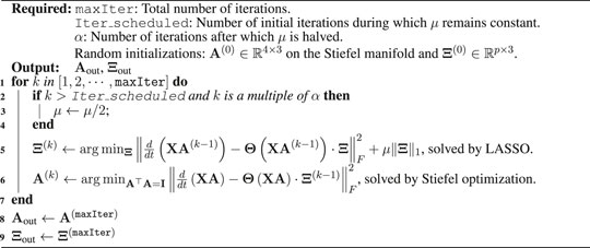
Algorithm 1.

4 Numerical results

In this section, we present numerical results on data-driven closure of moment systems (Examples 1–3) using the methodologies described in Section 3. To obtain the data, we first numerically solve the PDE Equation 1 with periodic boundary conditions and various ICs using an extended 4th-order Runge-Kutta method, the exponential integrator (ETDRK4) (see (Kassam and Trefethen, 2005) for a detailed explanation). The time series of the moments is subsequently extracted by numerical spatial integration according to Equations 2–5, with spatial derivatives computed using pseudo-spectral Fourier methods. We note once again that should the numerical data be replaced by “experimental” ones from a given physical process, the procedure can still be applied. Unless otherwise noted, the time series are evaluated at $N=\mathrm{16,000}$ uniformly spaced times $t=t_1,\dots ,t_N$, where $t_i=i\mathrm{\Delta }t$ and $\mathrm{\Delta }t=0.0025$.

4.1 Examples with analytical moment closure

We first examine Examples (1) and (2), where analytical (linear) closure exists for the chosen moments $\mathbf{x}=[I_1,V_0]$ (Example 1) and $\mathbf{x}=[I_2,V_1,K]$ (Example 2).

4.2 Example 1

Let the selected moments be $\mathbf{x}=[I_1,V_0]$. We construct the data matrices ${\mathbf{X}}^{(0)}=[{\mathbf{I}}_1^{(0)},{\mathbf{V}}_0^{(0)}]\in {\mathbb{R}}^{N\times 2}$ and ${\mathbf{X}}^{(1)}=[{\mathbf{I}}_1^{(1)},{\mathbf{V}}_0^{(1)}]\in {\mathbb{R}}^{N\times 2}$ from numerically solving the PDE Equation 1 with the ICs:

$u^{\left(1\right)}\left(x,0\right)={\pi }^{-1/4}\exp \left(-\frac{1}{2}{\left(x-5\right)}^2\right),$

$u^{\left(2\right)}\left(x,0\right)=\frac{1}{2}{\mathrm{s}\mathrm{e}\mathrm{c}\mathrm{h}}^2\left(x-5\right).$

We apply SINDy to this system using monomial libraries of degree up to $n\in \mathbb{N}$, ${\mathbf{\Theta }}_{\mathrm{deg}\le n}(\mathbf{x})$, as defined in Equation 9. We find that as long as $n\le 2$, SINDy applied to either data matrix ${\mathbf{X}}^{(0)}$ or ${\mathbf{X}}^{(1)}$ discovers the dynamics nearly perfectly. However, as we gradually expand the library ${\mathbf{\Theta }}_{\mathrm{deg}\le n}(\mathbf{x})$ by increasing $n$, SINDy applied to either ${\mathbf{X}}^{(0)}$ or ${\mathbf{X}}^{(1)}$ individually typically produces erroneous dynamics, regardless of how carefully the sparsity-promoting parameter is tuned. A typical negative result from SINDy applied to ${\mathbf{X}}^{(0)}$ with $n=3$ is presented in the Supplementary Material. This outcome is expected, as increasing the library size makes the problem more ill-posed, leading SINDy to overfit the data and produce incorrect dynamics.

To address the overfitting issue, we can enlarge the dataset by concatenating the data matrices ${\mathbf{X}}^{(0)}$ and ${\mathbf{X}}^{(1)}$ vertically, forming $\mathbf{X}={[{\mathbf{X}}^{(0)\top },{\mathbf{X}}^{(1)\top }]}^{\top }\in {\mathbb{R}}^{2N\times 2}$. When applying SINDy to this new data matrix $\mathbf{X}$ (considering boundary issues when taking finite differences), SINDy can now discover the correct dynamics that match Equation 6, even with a much larger library ${\mathbf{\Theta }}_{\mathrm{deg}\le n}(\mathbf{x})$ for $n$ up to 16. For example, when $n=16$, the output ODE from SINDy reads

$\left\{\begin{array}{cc}\hfill \frac{d{I}_1}{dt}& =1.000V_0,\hfill \\ \hfill \frac{d{V}_0}{dt}& =-1.000I_1,\hfill \end{array}\right.$

where the coefficients are rounded to three decimal places. This suggests the potential usefulness of concatenating different time series, especially in cases where one may not be familiar with the order of the relevant closure.

4.3 Example 2

For Example 2 with the selected moments $\mathbf{x}=[I_2,V_1,K]$, our findings are similar to those in Section 4.2. When applying SINDy to a data matrix from a single IC, SINDy discovers erroneous dynamics for the quadratic dictionary ${\mathbf{\Theta }}_{\mathrm{deg}\le 2}$. However, using larger data matrices from multiple ICs, SINDy can once again accurately identify the correct dynamics even with the larger dictionaries. Representative negative and positive results are presented in the Supplementary Material, similar to the previous example.

4.4 Examples where closure exists after coordinate transformations

We now turn to Example 3, where the selected moments are $\mathbf{x}=[I_2,V_1,K,J]$, and the moment system only closes after a coordinate transformation. Specifically, we consider the nonlinearity $g(\rho ,t)={\rho }^2$ in Equation 1, which satisfies the condition in Example 3. We collect the moment time series data by numerically solving the PDE with the following four distinct ICs, Equations 13–16:

$u^{\left(1\right)}\left(x,0\right)={\pi }^{-1/4}\exp \left(-\frac{1}{2}{\left(x-5\right)}^2\right),(13)$

$u^{\left(2\right)}\left(x,0\right)=1.88\exp \left(-\frac{1}{2}{\left(x-5\right)}^2\right),(14)$

$u^{\left(3\right)}\left(x,0\right)=1.88\left(\exp \left(-\frac{1}{2}{\left(x-5\right)}^2\right)+\exp \left(-{\left(x-2\right)}^2\right)\right),(15)$

$u^{\left(4\right)}\left(x,0\right)=1.88\left(\cos \left(2x\right)+\sin \left(2x\right)\right)\exp \left(-x^2\right).(16)$

We consider the following questions:

$•$ What insights can we gain by directly applying SINDy to this system with the selected moments $\mathbf{x}=[I_2,V_1,K,J]$, where a closure does not exist?

$•$ Can the method described in Section 3.2 correctly identify the coordinate transformation that closes the moment system?

We note that normalized moment time series are used as input for SINDy, as a way of incorporating feature scaling. This is an important aspect that ensures that all the relevant quantities are considered on “equal footing,” when the sparse regression step takes place.

4.5 SINDy with linear library ${\mathbf{\Theta }}_{\mathrm{deg}=1}(\mathbf{x})$

We begin by applying SINDy with a linear library ${\mathbf{\Theta }}_{\mathrm{deg}=1}(\mathbf{x})$ to the moment time series data from IC Equation 14. The resulting equations are:

$\left\{\begin{array}{cc}\hfill \frac{d{I}_2}{dt}& =1.000V_1,\hfill \\ \hfill \frac{d{V}_1}{dt}& =-2.000I_2+4.000K+3.998J,\hfill \\ \hfill \frac{dK}{dt}& =-0.569V_1,\hfill \\ \hfill \frac{dJ}{dt}& =0.069V_1.\hfill \end{array}\right.(17)$

The coefficients are rounded to three decimal places. The first four panels of Figure 1 compare the “ground-truth” time-evolution data of $[I_2,V_1,K,J]$ obtained from PDE integration (red curves) and the definition of these quantities through Equations 2–5 with those from integrating the SINDy-predicted ODEs Equation 17 (blue curves). While the SINDy-predicted time evolution of $[I_2,V_1]$ closely matches the ground truth, there is a significant discrepancy for the moments $[K,J]$ in Figure 1. Accordingly, the SINDy-predicted dynamics is not accurate for the original coordinates $\mathbf{x}=[I_2,V_1,K,J]$.

Figure 1

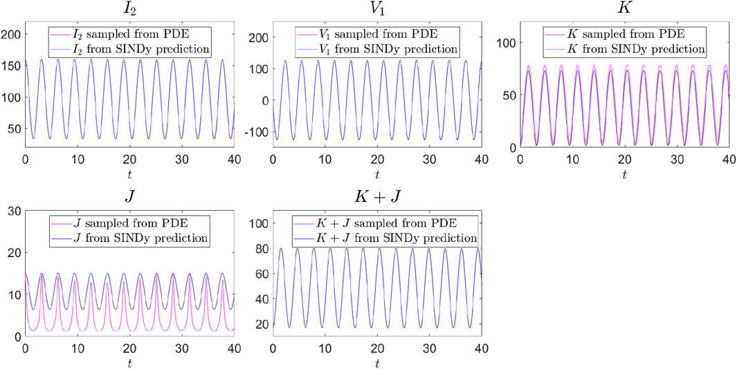
Figure 1. Comparison of the ground-truth and SINDy-predicted time evolutions of $[I_2,V_1,K,J,K+J]$. SINDy is trained only on the selected moments $\mathbf{x}=[I_2,V_1,K,J]$, where a closure does not exist, using a linear library ${\mathbf{\Theta }}_{\mathrm{deg}=1}(\mathbf{x})$. Interestingly, SINDy can “afford” to sacrifice accurate prediction for $K$ and $J$ individually, provided that it captures the correct dynamics for $E=K+J$, suggesting in this way the proper coordinate transformation under which a closure does exist. For the physical meanings of the moments in this figure, please refer to Equations 2–5 and the paragraph thereafter.

Nevertheless, interestingly, if we add the ODE for $K$ with that for $J$ in Equation 17, which corresponds to the correct coordinate transformation for closure, we obtain:

$\left\{\begin{array}{cc}\frac{d{I}_2}{dt}\hfill & =1.000V_1,\hfill \\ \frac{d{V}_1}{dt}\hfill & =-2.000I_2+4.000K+3.998J,\hfill \\ \hfill \frac{d\left(K+J\right)}{dt}& =-0.500V_1.\hfill \end{array}\right.(18)$

Equation 18 closely matches the ground-truth moment system Equation 7. The last panel of Figure 1 shows that the predicted time evolution of $K+J$ aligns perfectly with the ground truth, even though SINDy does not accurately recover those of $K$ and $J$ individually. This finding is intriguing because, even when SINDy is applied to the original coordinates $[I_2,V_1,K,J]$ without closure, it “strategically chooses” to sacrifice accuracy for $K$ and $J$ but indirectly captures the correct dynamics when considering the proper coordinate transformation $E=K+J$. Moreover, a similar pattern is consistently observed when applying SINDy to the moments simulated from the other three ICs. The results are shown in the Supplementary Material. We have also provided an analogous example for 2D NLS equations. For details, please refer to Section 3 of the Supplementary Material. Indeed, this clearly illustrates that the methodology presented herein is not in any fundamental way limited to 1D NLS models, but can be extended to higher dimensional ones, as may be deemed desirable.

4.6 SINDy with quadratic library ${\mathbf{\Theta }}_{\mathrm{deg}\le 2}(\mathbf{x})$

Next, we investigate the performance of SINDy with an expanded quadratic library ${\mathbf{\Theta }}_{\mathrm{deg}\le 2}(\mathbf{x})$ applied to the moment time series with the same IC Equation 14. The predicted ODEs now become:

$\left\{\begin{array}{cc}\hfill \frac{d{I}_2}{dt}& =1.000V_1,\hfill \\ \hfill \frac{d{V}_1}{dt}& =-2.000I_2+4.000K+3.998J,\hfill \\ \hfill \frac{dK}{dt}& =-0.174V_1-0.003V_{1}K-0.083V_{1}J,\hfill \\ \hfill \frac{dJ}{dt}& =-0.002I_2{V}_1+0.082V_{1}J.\hfill \end{array}\right.(19)$

As before, if we add the predicted dynamics of $K$ and $J$ in Equation 19, we obtain:

$\left\{\begin{array}{cc}\frac{d{I}_2}{dt}\hfill & =1.000V_1,\hfill \\ \frac{d{V}_1}{dt}\hfill & =-2.000I_2+4.000K+3.998J,\hfill \\ \hfill \frac{d\left(K+J\right)}{dt}& =-0.174V_1-0.003V_{1}K-0.002I_2{V}_1-0.001V_{1}J.\hfill \end{array}\right.(20)$

Unlike the previous case with ${\mathbf{\Theta }}_{\mathrm{deg}=1}(\mathbf{x})$, the SINDy-predicted governing Equation 20 using the expanded library ${\mathbf{\Theta }}_{\mathrm{deg}\le 2}(\mathbf{x})$ after the (theoretically motivated) coordinate transformation $E=K+J$ still fails to match the ground truth ODE Equation 7 and remains unclosed (i.e., the third equation in Equation 20 cannot be written using only $I_2$, $V_1$, and $E=K+J$). Specifically, the coefficient of $V_1$ in Equation 20 is $-0.174$, deviating substantially from that of $-0.5$ in the ground truth. Although the coefficients for the additional terms ($V_{1}K$, $I_2{V}_1$, and $V_{1}J$) are relatively small, their presence hinders the accurate recovery of the correct coefficient for $V_1$.

Figure 2 compares the ground-truth time evolutions of $[I_2,V_1,K,J,E=K+J]$ obtained from PDE integration with their SINDy-predicted dynamics after integrating Equations 19, 20. Similar to Figure 1, SINDy with the quadratic library ${\mathbf{\Theta }}_{\mathrm{deg}\le 2}(\mathbf{x})$ applied to the unclosed moments $[I_2,V_1,K,J]$ sacrifices the exact recovery of the time evolution of $J$ and $K$, but indirectly captures the correct time evolution of $E=J+K$. However, unlike the linear library case in Section 4.5, SINDy with the quadratic library can yield the correct time evolution of $E=K+J$ but fails to uncover the correct governing equation for $E$ [Equation 20] due to the expanded library size, leading to overfitting issues discussed above.

Figure 2

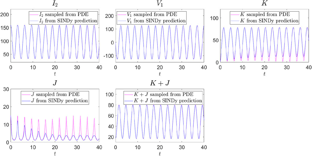
Figure 2. Comparison of the ground-truth and SINDy-predicted time evolutions of $[I_2,V_1,K,J,K+J]$. SINDy is trained only on the selected moments $\mathbf{x}=[I_2,V_1,K,J]$, where a closure does not exist, using a quadratic library ${\mathbf{\Theta }}_{\mathrm{deg}\le 2}(\mathbf{x})$. Similar to Figure 1, SINDy sacrifices accurate prediction for $K$ and $J$ individually but indirectly captures the correct time evolution of $E=K+J$.

Here, we see a key complication within SINDy that has been also present in works such as (Champion et al., 2019) and especially (Bakarji et al., 2022), namely the methodology is likely to result in ODE models that are proximal to the theoretically expected ones, but not identical to them. This, in turn, may result in a nontrivial error outside of the training set. Especially when the library at hand is “richer” than the terms expected to be present, unfortunately, it does not generically seem that the reduced, theoretically expected model will be discovered. Rather, our results suggest that it is possible that the additional “wealth” of the libraries used can be leveraged to approximate the data via different (nonlinear) dependent variable combinations.

As an even more problematic example, applying SINDy with a quadratic library to the moment time series generated from another IC Equation 16 results in a predicted ODE system that not only fails to match the ground truth, even after the theoretically suggested coordinate transformation $K+J$, but also causes the ODE system to blow up in finite time. For a detailed discussion, we refer the interested reader to the Supplementary Material.

4.7 Stiefel optimization for discovering coordinate transformations

Next, we test the methodology from Section 3.2 to discover the coordinate transformation needed to close the moment system.

Case 1: $\mu =0$. We first consider the case where the hyperparameter $\mu$ in Equation 12 is set to $\mu =0$, i.e., we do not promote sparsity in the matrix $\mathbf{\Xi }$. We use the linear library $\mathbf{\Theta }(\mathbf{x})={\mathbf{\Theta }}_{\mathrm{deg}=1}(\mathbf{x})$, and set the maximum number of iterations to $\mathtt{m}\mathtt{a}\mathtt{x}\mathtt{I}\mathtt{t}\mathtt{e}\mathtt{r}=150$ in Algorithm 1. The algorithm produces the following outputs

${\mathbf{A}}_{out}\approx \left[\begin{array}{ccc}\hfill -0.973\hfill & \hfill 0.179\hfill & \hfill 0.144\hfill \\ \hfill -0.169\hfill & \hfill -0.982\hfill & \hfill 0.083\hfill \\ \hfill -0.111\hfill & \hfill -0.040\hfill & \hfill -0.697\hfill \\ \hfill -0.111\hfill & \hfill -0.040\hfill & \hfill -0.697\hfill \end{array}\right],{\mathbf{\Xi }}_{out}\approx \left[\begin{array}{ccc}\hfill -0.024\hfill & \hfill -1.076\hfill & \hfill 0.005\hfill \\ \hfill 1.016\hfill & \hfill 0.470\hfill & \hfill -0.540\hfill \\ \hfill 0.913\hfill & \hfill 5.778\hfill & \hfill -0.446\hfill \end{array}\right].(21)$

The coefficients are rounded to three decimal places. On the other hand, the “ground-truth” coordinate transformation ${\mathbf{A}}_{gt}$ (after normalization to satisfy the Stiefel manifold constraint) and the corresponding dynamics ${\mathbf{A}}_{gt}$ according to Equation 7 are:

${\mathbf{A}}_{gt}=\left[\begin{array}{ccc}\hfill 1\hfill & \hfill 0\hfill & \hfill 0\hfill \\ \hfill 0\hfill & \hfill 1\hfill & \hfill 0\hfill \\ \hfill 0\hfill & \hfill 0\hfill & \hfill \frac{1}{\sqrt{2}}\hfill \\ \hfill 0\hfill & \hfill 0\hfill & \hfill \frac{1}{\sqrt{2}}\hfill \end{array}\right]\approx \left[\begin{array}{ccc}\hfill 1\hfill & \hfill 0\hfill & \hfill 0\hfill \\ \hfill 0\hfill & \hfill 1\hfill & \hfill 0\hfill \\ \hfill 0\hfill & \hfill 0\hfill & \hfill 0.707\hfill \\ \hfill 0\hfill & \hfill 0\hfill & \hfill 0.707\hfill \end{array}\right],{\mathbf{\Xi }}_{gt}=\left[\begin{array}{ccc}\hfill 0\hfill & \hfill -2\hfill & \hfill 0\hfill \\ \hfill 1\hfill & \hfill 0\hfill & \hfill -\frac{1}{2\sqrt{2}}\hfill \\ \hfill 0\hfill & \hfill 4\sqrt{2}\hfill & \hfill 0\hfill \end{array}\right]\approx \left[\begin{array}{ccc}\hfill 0\hfill & \hfill -2\hfill & \hfill 0\hfill \\ \hfill 1\hfill & \hfill 0\hfill & \hfill -0.354\hfill \\ \hfill 0\hfill & \hfill 5.657\hfill & \hfill 0\hfill \end{array}\right](22)$

At first glance, the predicted solution Equation 21 appears different from the ground truth in Equation 22. However, after a further change of coordinates using

$\mathbf{O}=\left[\begin{array}{ccc}\hfill -0.973\hfill & \hfill -0.169\hfill & \hfill -0.156\hfill \\ \hfill 0.179\hfill & \hfill -0.982\hfill & \hfill -0.0565\hfill \\ \hfill 0.144\hfill & \hfill 0.0830\hfill & \hfill -0.986\hfill \end{array}\right]\in \text{O}\left(3\right),$

we have

${\mathbf{A}}_{out}\mathbf{O}=\left[\begin{array}{ccc}\hfill 1.000\hfill & \hfill -0.000\hfill & \hfill 0.000\hfill \\ \hfill 0.000\hfill & \hfill 1.000\hfill & \hfill -0.000\hfill \\ \hfill 0.000\hfill & \hfill -0.000\hfill & \hfill 0.707\hfill \\ \hfill 0.000\hfill & \hfill 0.000\hfill & \hfill 0.707\hfill \end{array}\right]\approx {\mathbf{A}}_{gt},{\mathbf{O}}^{\top }{\mathbf{\Xi }}_{out}\mathbf{O}=\left[\begin{array}{ccc}\hfill 0.000\hfill & \hfill -2.000\hfill & \hfill 0.000\hfill \\ \hfill 1.000\hfill & \hfill 0.000\hfill & \hfill -0.354\hfill \\ \hfill 0.000\hfill & \hfill 5.657\hfill & \hfill 0.000\hfill \end{array}\right]\approx {\mathbf{\Xi }}_{gt}.$

Hence, according to Remark 2, $({\mathbf{A}}_{out},{\mathbf{\Xi }}_{out})$ and $({\mathbf{A}}_{gt},{\mathbf{\Xi }}_{gt})$ are equivalent solutions, and our method successfully predicts the correct coordinate transformation ${\mathbf{A}}_{out}$ to close the moment system. However, as expected, due to $\mu =0$, the linear combination matrix ${\mathbf{\Xi }}_{out}$ of the transformed dictionary is not sparse.

Case 2: $\mu >0$. We next explore the case when $\mu \ne 0$ in Equation 12. We use the same linear library $\mathbf{\Theta }(\mathbf{x})={\mathbf{\Theta }}_{\mathrm{deg}=1}(\mathbf{x})$, and $\mu$ is initially set to $\mu =1$. In Algorithm 1, we set $\mathtt{m}\mathtt{a}\mathtt{x}\mathtt{I}\mathtt{t}\mathtt{e}\mathtt{r}=1000$, $\mathtt{I}\mathtt{t}\mathtt{e}\mathtt{r}\text{\_}\mathtt{s}\mathtt{c}\mathtt{h}\mathtt{e}\mathtt{d}\mathtt{u}\mathtt{l}\mathtt{e}\mathtt{d}=400$, and $\alpha =20$. The algorithm returns

${\tilde{\mathbf{A}}}_{out}\approx \left[\begin{array}{ccc}\hfill -1.000\hfill & \hfill 0.000\hfill & \hfill 0.030\hfill \\ \hfill 0.000\hfill & \hfill -0.100\hfill & \hfill 0.002\hfill \\ \hfill -0.021\hfill & \hfill -0.001\hfill & \hfill -0.707\hfill \\ \hfill -0.021\hfill & \hfill -0.001\hfill & \hfill -0.707\hfill \end{array}\right],{\tilde{\mathbf{\Xi }}}_{out}\approx \left[\begin{array}{ccc}\hfill 0.000\hfill & \hfill -1.830\hfill & \hfill 0.003\hfill \\ \hfill 1.000\hfill & \hfill 0.011\hfill & \hfill -0.383\hfill \\ \hfill 0.000\hfill & \hfill 5.714\hfill & \hfill -0.010\hfill \end{array}\right].(23)$

Similarly, after a further change of coordinates using:

$\tilde{\mathbf{O}}=\left[\begin{array}{ccc}\hfill -1.000\hfill & \hfill 0.000\hfill & \hfill -0.030\hfill \\ \hfill 0.000\hfill & \hfill -1.000\hfill & \hfill -0.002\hfill \\ \hfill 0.030\hfill & \hfill 0.002\hfill & \hfill -1\hfill \end{array}\right]\in \text{O}\left(3\right),$

we again have

${\tilde{\mathbf{A}}}_{out}\tilde{\mathbf{O}}=\left[\begin{array}{ccc}\hfill 1.000\hfill & \hfill -0.000\hfill & \hfill 0.000\hfill \\ \hfill 0.000\hfill & \hfill 1.000\hfill & \hfill -0.000\hfill \\ \hfill 0.000\hfill & \hfill -0.000\hfill & \hfill 0.707\hfill \\ \hfill 0.000\hfill & \hfill 0.000\hfill & \hfill 0.707\hfill \end{array}\right]\approx {\mathbf{A}}_{gt},{\tilde{\mathbf{O}}}^{\top }{\tilde{\mathbf{\Xi }}}_{out}\tilde{\mathbf{O}}=\left[\begin{array}{ccc}\hfill 0.000\hfill & \hfill -2.000\hfill & \hfill 0.000\hfill \\ \hfill 1.000\hfill & \hfill 0.000\hfill & \hfill -0.354\hfill \\ \hfill 0.000\hfill & \hfill 5.657\hfill & \hfill 0.000\hfill \end{array}\right]\approx {\mathbf{\Xi }}_{gt}.$

Note that the result $({\tilde{\mathbf{A}}}_{out},{\tilde{\mathbf{\Xi }}}_{out})$ in Equation 23 for $\mu >0$ is much closer to the ground truth $({\mathbf{A}}_{gt},{\mathbf{\Xi }}_{gt})$ in Equation 22, compared to $({\mathbf{A}}_{out},{\mathbf{\Xi }}_{out})$ in Equation 21 with $\mu =0$. This demonstrates that a positive $\mu$ with annealed optimization not only discovers the correct coordinate transformation to close the system but also achieves a sparser solution for $\mathbf{\Xi }$, reducing the number of terms on the right-hand side of the moment ODE system.

4.8 An example of unclosed moment system

Finally, we present a case without analytical closure. Our “data-driven closure” aims to provide an accurate, reduced-order description of the PDE by approximating the evolution of the moment systems. In principle, this is the type of problem that we are aiming for, namely the discovery of potential moment closures when these may not be analytically available; the examples presented previously are valuable benchmarks to raise the complications that may emerge when one seeks to use this type of methodology in systems where the answer may be unknown and what credibility one may wish to assign to the obtained results.

Specifically, we consider an NLS Equation 1 with a time-dependent nonlinearity:

$g\left(\rho ,t\right)=\left(\sin \left(t\right)+2\right){\left|\rho \right|}^2.(24)$

Notice that such time-dependent nonlinearities are well-known for some time in atomic physics settings (Donley et al., 2001; Staliunas et al., 2002) (and continue to yield novel insights to this day (Shagalov and Friedland, 2024)) and similar dynamical scenarios have been considered in nonlinear optics (Centurion et al., 2006; Zhang et al., 2021).

Moment systems with such nonlinearity will not close to the best of our knowledge, so we aim to numerically approximate form of the dynamics of the moments $\mathbf{x}=[I_2,V_1,E]$, where $E=K+J$. We consider the following three ICs:

$u_1\left(x,0\right)=1.88\exp \left(-\frac{1}{2}{\left(x-5\right)}^2\right),(25)$

$u_2\left(x,0\right)=1.88\left(\cos \left(2x\right)+\sin \left(2x\right)\right)\exp \left(-x^2\right),(26)$

$u_3\left(x,0\right)=\exp \left(-0.1x^2\right)\exp \left(0.1i{x}^2\right).(27)$

Notably, the IC Equation 27 includes a quadratic phase, motivated by the quadratic phase approximation (QPA) ansatz for NLS equations discussed by (Pérez-García et al., 2007). It also includes regular, smooth localized initial conditions, as well as one involving Fourier mode oscillations, modulated by the Gaussian term. We expect the SINDy-predicted dynamics to vary with the different ICs of Equations 25–27, hence the relevant choices.

Due to the periodic nature of the nonlinearity $g$ in Equation 24, we expect the moment system to be non-autonomous and exhibit an oscillatory pattern. To capture this, we introduce the following two “auxiliary moments”:

$\left\{\begin{array}{cc}\hfill H& =\sin \left(t\right)+2,\hfill \\ \hfill Q& =\cos \left(t\right)+2.\hfill \end{array}\right.$

Naturally, one can observe that these are inspired by the nature of $g(\rho ,t)$. However, one can envision the use of Fourier modes even if the mathematical model was not known or if the data stemmed from experimental observations.

We then apply SINDy with a linear library ${\mathbf{\Theta }}_{\mathrm{deg}=1}(\tilde{\mathbf{x}})$ to the expanded moment systems $\tilde{\mathbf{x}}=[\mathbf{x},H,Q]=[I_2,V_1,E,H,Q]$. The time series data of the moments are collected by integrating the PDE up to $T=20$. The exact SINDy-predicted ODEs for all three ICs are presented in the Supplementary Material.

To test the accuracy of the predicted moment systems, we integrate the SINDy-predicted ODEs into the future, up to $T=100$. Figure 3 compares the ground-truth and SINDy-predicted time evolutions for the three ICs Equations 25–27. In all cases, the model closely matches the ground truth up to $T=100$. Indeed, this is well past the training time of $T=20$ and thus provides a satisfactory reduced-order description of the underlying PDE effective moment dynamics. Thus, despite the potential shortcomings of the method which we tried to present in an unbiased fashion in case examples where the analytical theory helps assess them, we still find it to be a worthwhile tool to consider. I.e., from a data-driven perspective, it can be seen to potentially provide an effective, low-dimensional dynamical representation of the associated high-dimensional PDE dynamics.

Figure 3

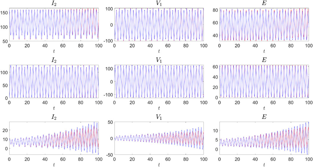
Figure 3. Comparison between the ground-truth time evolution (in red) and the SINDy-predicted evolution (in blue). Training data were obtained by integrating the NLS equation up to $T=20$ using the initial conditions of Equations 25–27. In all cases (displayed in three different rows), the SINDy-predicted moment dynamics closely match the ground truth, well past the time frame of the training data, offering a satisfactory reduced-order description of the underlying PDE through the corresponding moment systems.

5 Conclusion and future directions

This study explores a data-driven approach to identifying moment equations in nonlinear Schrödinger models. This paves the way more generally towards the use of similar methods in nonlinear PDEs which may feature similar wave phenomena. We applied the relevant sparse regression/optimization methodology aiming to rediscover known analytical closures (progressively extending considerations to more complex settings), addressed overfitting by augmenting datasets with multiple initial conditions, and identified suitable coordinate transformations for systems requiring them so as to bring forth the reduced or analytically tractable form of the dynamics. Additionally, we demonstrated that our approach could provide a reduced-order description of systems without analytical closures by approximating the evolution of the moment systems. Our findings show that this data-driven method can capture complex dynamics in NLS models and offer insights for various physical applications, possibly well past the training time used for the data-driven methods.

Future work will focus on extending our method to more complex PDEs and exploring its applicability to other types of nonlinear dynamical high-dimensional models, such as, e.g., the ones we mentioned in the context Fisher-KPP models and their applications to brain tumor dynamics, as analyzed, e.g., in (Belmonte-Beitia et al., 2014). Another possible avenue is to, instead of recovering the moment systems through numerical differentiation of the moment time series (as done in SINDy), leverage numerical integration into future time of a suitably augmented system. This approach, similar to Neural ODEs (Chen et al., 2018) and shooting methods, can help avoid producing predicted ODEs that blow up in finite time which SINDy may produce (see details in Section 4.2.2 and the Supplementary Material). Additionally, we plan to develop techniques to identify nonlinear coordinate transformations that can close the moment system, further enhancing the applicability of our method. Lastly, one can envision such classes of techniques for obtaining additional reduced features of solitary waves, such as data-driven variants of the variational approximation (Malomed, 2002), or data-driven models of soliton interaction dynamics (Manton, 1979; Kevrekidis et al., 2004; Ma et al., 2016).

Data availability statement

The original contributions presented in the study are included in the article/Supplementary Material, further inquiries can be directed to the corresponding author.

Author contributions

SY: Formal Analysis, Investigation, Methodology, Software, Writing–original draft. SC: Formal Analysis, Investigation, Methodology, Software, Writing–original draft. WZ: Conceptualization, Funding acquisition, Methodology, Writing–review and editing. PK: Conceptualization, Funding acquisition, Methodology, Supervision, Writing–review and editing.

Funding

The author(s) declare that financial support was received for the research, authorship, and/or publication of this article. This material is based upon work supported by the U.S. National Science Foundation under the awards PHY-2110030 and DMS-2204702 (PGK), as well as DMS-2052525, DMS-2140982, and DMS2244976 (WZ).

Conflict of interest

The authors declare that the research was conducted in the absence of any commercial or financial relationships that could be construed as a potential conflict of interest.

Publisher’s note

All claims expressed in this article are solely those of the authors and do not necessarily represent those of their affiliated organizations, or those of the publisher, the editors and the reviewers. Any product that may be evaluated in this article, or claim that may be made by its manufacturer, is not guaranteed or endorsed by the publisher.

Supplementary material

The Supplementary Material for this article can be found online at: https://www.frontiersin.org/articles/10.3389/fphot.2024.1444993/full#supplementary-material

References

Ablowitz, M. (2011). Nonlinear dispersive waves, asymptotic analysis and solitons. Cambridge: Cambridge University Press. doi:10.1017/cbo9780511998324

CrossRef Full Text | Google Scholar

Ablowitz, M., and Clarkson, P. (1991). “Solitons, nonlinear evolution equations, and inverse scattering,” in 149 of London math. Soc. Lecture note series. Cambridge: Cambridge U. Press.

Google Scholar

Ablowitz, M., Prinari, B., and Trubatch, A. (2004). Discrete and continuous nonlinear schrödinger systems. Cambridge: Cambridge University Press.

Google Scholar

Absil, P.-A., Mahony, R., and Sepulchre, R. (2008). Optimization algorithms on matrix manifolds. Princeton University Press.

Google Scholar

Bakarji, J., Champion, K. P., Kutz, J. N., and Brunton, S. L. (2022). Discovering governing equations from partial measurements with deep delay autoencoders. CoRR abs/2201, 05136. doi:10.1098/rspa.2023.0422

CrossRef Full Text | Google Scholar

Belmonte-Beitia, J., Calvo, G. F., and Pérez-García, V. M. (2014). Effective particle methods for Fisher–Kolmogorov equations: theory and applications to brain tumor dynamics. Commun. Nonlinear Sci. Numer. Simul. 19, 3267–3283. doi:10.1016/j.cnsns.2014.02.004

CrossRef Full Text | Google Scholar

Brunton, S. L., Proctor, J. L., and Kutz, J. N. (2016). Discovering governing equations from data by sparse identification of nonlinear dynamical systems, 3932–3937.

CrossRef Full Text | Google Scholar

Centurion, M., Porter, M. A., Kevrekidis, P. G., and Psaltis, D. (2006). Nonlinearity management in optics: experiment, theory, and simulation. Phys. Rev. Lett. 97, 033903. doi:10.1103/PhysRevLett.97.033903

PubMed Abstract | CrossRef Full Text | Google Scholar

Champion, K., Lusch, B., Kutz, J. N., and Brunton, S. L. (2019). Data-driven discovery of coordinates and governing equations. Proc. Natl. Acad. Sci. 116, 22445–22451. doi:10.1073/pnas.1906995116

PubMed Abstract | CrossRef Full Text | Google Scholar

Chen, R. T., Rubanova, Y., Bettencourt, J., and Duvenaud, D. K. (2018). Neural ordinary differential equations. Adv. neural Inf. Process. Syst. 31. doi:10.48550/arXiv.1806.07366

CrossRef Full Text | Google Scholar

De Koster, P., and Wahls, S. (2024). Data-driven identification of the spectral operator in AKNS Lax pairs using conserved quantities. Wave Motion 127, 103273. doi:10.1016/j.wavemoti.2024.103273

CrossRef Full Text | Google Scholar

Donley, E. A., Claussen, N. R., Cornish, S. L., Roberts, J. L., Cornell, E. A., and Wieman, C. E. (2001). Dynamics of collapsing and exploding Bose–Einstein condensates. Nature 412, 295–299. doi:10.1038/35085500

PubMed Abstract | CrossRef Full Text | Google Scholar

Edelman, A., Arias, T. A., and Smith, S. T. (1998). The geometry of algorithms with orthogonality constraints. SIAM J. Matrix Analysis Appl. 20, 303–353. doi:10.1137/s0895479895290954

CrossRef Full Text | Google Scholar

Feliu-Faba, J., Fan, Y., and Ying, L. (2020). Meta-learning pseudo-differential operators with deep neural networks. J. Comput. Phys. 408, 109309. doi:10.1016/j.jcp.2020.109309

CrossRef Full Text | Google Scholar

García-Ripoll, J., and Pérez-García, V. (1999). The moment method in general nonlinear Schrödinger equations

Google Scholar

Hasegawa, A., and Kodama, Y. (1995). Solitons in optical communications. Oxford: Clarendon Press.

Google Scholar

Infeld, E., and Rowlands, G. (2000). Nonlinear waves, solitons and chaos. Cambridge: Cambridge University Press.

Google Scholar

Karjanto, N. (2024). Modeling wave packet dynamics and exploring applications: a comprehensive guide to the nonlinear Schrödinger equation. Mathematics 12, 744. doi:10.3390/math12050744

CrossRef Full Text | Google Scholar

Karniadakis, G., Kevrekidis, I., Lu, L., Perdikaris, P., Wang, S., and Yang, L. (2021). Physics-informed machine learning. Nat. Rev. Phys. 3, 422–440. doi:10.1038/s42254-021-00314-5

CrossRef Full Text | Google Scholar

Kassam, A.-K., and Trefethen, L. N. (2005). Fourth-order time-stepping for stiff PDEs. SIAM J. Sci. Comput. 26, 1214–1233. doi:10.1137/s1064827502410633

CrossRef Full Text | Google Scholar

Kevrekidis, P. G., Frantzeskakis, D. J., and Carretero-González, R. (2015). The defocusing nonlinear schrödinger equation. Philadelphia: SIAM.

Google Scholar

Kevrekidis, P. G., Khare, A., and Saxena, A. (2004). Solitary wave interactions in dispersive equations using Manton’s approach. Phys. Rev. E 70, 057603. doi:10.1103/PhysRevE.70.057603

PubMed Abstract | CrossRef Full Text | Google Scholar

Kivshar, Y. S., and Agrawal, G. P. (2003). Optical solitons: from fibers to photonic crystals. Academic Press. doi:10.1016/B978-0-12-410590-4.X5000-1

CrossRef Full Text | Google Scholar

Kono, M., and Skorić, M. (2010). Nonlinear physics of plasmas. Heidelberg: Springer-Verlag.

Google Scholar

Krippendorf, S., Lüst, D., and Syvaeri, M. (2021). Integrability ex machina. Fortschritte Phys. 69, 2100057. doi:10.1002/prop.202100057

CrossRef Full Text | Google Scholar

Li, Z., Kovachki, N., Azizzadenesheli, K., Liu, B., Bhattacharya, K., Stuart, A., et al. (2021). “Fourier neural operator for parametric partial differential equations,” in International Conference on Learning Representations.

Google Scholar

Liu, X., Xiao, N., and Xiang Yuan, Y. (2021). A penalty-free infeasible approach for a class of nonsmooth optimization problems over the Stiefel manifold. J. Sci. Comput. 99, 30. doi:10.1007/s10915-024-02495-4

CrossRef Full Text | Google Scholar

Liu, Z., Madhavan, V., and Tegmark, M. (2022). Machine learning conservation laws from differential equations. Phys. Rev. E 106, 045307. doi:10.1103/physreve.106.045307

PubMed Abstract | CrossRef Full Text | Google Scholar

Liu, Z., and Tegmark, M. (2021). Machine learning conservation laws from trajectories. Phys. Rev. Lett. 126, 180604. doi:10.1103/PhysRevLett.126.180604

PubMed Abstract | CrossRef Full Text | Google Scholar

Liu, Z., and Tegmark, M. (2022). Machine learning hidden symmetries. Phys. Rev. Lett. 128, 180201. doi:10.1103/PhysRevLett.128.180201

PubMed Abstract | CrossRef Full Text | Google Scholar

Lu, L., Meng, X., Mao, Z., and Karniadakis, G. (2021). DeepXDE: a deep learning library for solving differential equations. SIAM Rev. 63, 208–228. doi:10.1137/19m1274067

CrossRef Full Text | Google Scholar

Ma, M., Navarro, R., and Carretero-González, R. (2016). Solitons riding on solitons and the quantum Newton’s cradle. Phys. Rev. E 93, 022202. doi:10.1103/PhysRevE.93.022202

PubMed Abstract | CrossRef Full Text | Google Scholar

Malomed, B. A. (2002). Progress in optics (Elsevier). Var. methods nonlinear fiber Opt. Relat. fields 43, 69–191. doi:10.1016/S0079-6638(02)80026-9

CrossRef Full Text | Google Scholar

Manton, N. (1979). An effective Lagrangian for solitons. Nucl. Phys. B 150, 397–412. doi:10.1016/0550-3213(79)90309-2

CrossRef Full Text | Google Scholar

Oviedo, H., and Dalmau, O. (2019). “A scaled gradient projection method for minimization over the Stiefel manifold,” in Advances in soft computing. Editors L. Martínez-Villaseñor, I. Batyrshin, and A. Marín-Hernández (Cham: Springer International Publishing), 239–250.

CrossRef Full Text | Google Scholar

Pérez-García, V., Torres, P., and Montesinos, G. (2007). The method of moments for nonlinear Schrödinger equations: theory and applications. SIAM J. Appl. Math. 67, 990–1015. doi:10.1137/050643131

CrossRef Full Text | Google Scholar

Pethick, C. J., and Smith, H. (2002). Bose–einstein condensation in Dilute Gases. Cambridge, United Kingdom: Cambridge University Press.

Google Scholar

Pitaevskii, L., and Stringari, S. (2003). Bose-Einstein condensation. Oxford: Oxford University Press.

Google Scholar

Raissi, M., Perdikaris, P., and Karniadakis, G. E. (2019). Physics-informed neural networks: a deep learning framework for solving forward and inverse problems involving nonlinear partial differential equations. J. Comput. Phys. 378, 686–707. doi:10.1016/j.jcp.2018.10.045

CrossRef Full Text | Google Scholar

Schaeffer, H. (2017). Learning partial differential equations via data discovery and sparse optimization. Proc. R. Soc. A Math. Phys. Eng. Sci. 473, 20160446. doi:10.1098/rspa.2016.0446

PubMed Abstract | CrossRef Full Text | Google Scholar

Shagalov, A. G., and Friedland, L. (2024). Autoresonant generation of solitons in Bose-Einstein condensates by modulation of the interaction strength. Phys. Rev. E 109, 014201. doi:10.1103/PhysRevE.109.014201

PubMed Abstract | CrossRef Full Text | Google Scholar

Staliunas, K., Longhi, S., and de Valcárcel, G. J. (2002). Faraday patterns in Bose-Einstein condensates. Phys. Rev. Lett. 89, 210406. doi:10.1103/PhysRevLett.89.210406

PubMed Abstract | CrossRef Full Text | Google Scholar

Sulem, C., and Sulem, P. (1999). The nonlinear Schrödinger equation: self-focusing and wave collapse. New York: Springer.

Google Scholar

Tibshirani, R. (1996). Regression shrinkage and selection via the lasso. J. R. Stat. Soc. Ser. B Stat. Methodol. 58, 267–288. doi:10.1111/j.2517-6161.1996.tb02080.x

CrossRef Full Text | Google Scholar

Xiao, N., Liu, X., and Yuan, Y.-x. (2020). A class of smooth exact penalty function methods for optimization problems with orthogonality constraints. Optim. Methods Softw. 37, 1205–1241. doi:10.1080/10556788.2020.1852236

CrossRef Full Text | Google Scholar

Zhang, S., Fu, Z., Zhu, B., Fan, G., Chen, Y., Wang, S., et al. (2021). Solitary beam propagation in periodic layered Kerr media enables high-efficiency pulse compression and mode self-cleaning. Light Sci. and Appl. 10, 53. doi:10.1038/s41377-021-00495-9

PubMed Abstract | CrossRef Full Text | Google Scholar

Zhu, W., Zhang, H.-K., and Kevrekidis, P. G. (2023). Machine learning of independent conservation laws through neural deflation. Phys. Rev. E 108, L022301. doi:10.1103/PhysRevE.108.L022301

PubMed Abstract | CrossRef Full Text | Google Scholar