 Ella Poppy Tanner
 Harry Ewin
 Johannes J. Viljoen
 Robert J. W. Brewin
- Centre for Geography and Environmental Science, University of Exeter, Penryn, Cornwall, United Kingdom
Phytoplankton occupy the oceans’ euphotic zone and are responsible for its primary production; thus, our ability to monitor their patterns of abundance and physiology is vital for tracking ocean health. Ocean colour sensors mounted on satellites can monitor the surface patterns of phytoplankton daily at global scales but cannot see into the subsurface. Autonomous robotic platforms, like Biogeochemical-Argo (BGC-Argo) profiling floats, do not have the coverage of satellites but can monitor the subsurface. Combining these methods can help track phytoplankton patterns throughout the euphotic zone. In this study, using a global array of BGC-Argo floats (76,043 profiles, spanning from 2010 to 2023), we revisit empirical relationships between the surface and column-integrated concentrations of chlorophyll-a (a proxy for phytoplankton abundance and physiology), originally developed using ship-based profiling data. We show that these relationships agree well with BGC-Argo float data. We then extend the relationships, removing the binary switch in parameters between mixed and stratified waters and trophic conditions such that the column-integrated chlorophyll-a concentration can be estimated as a continuous function of surface chlorophyll-a and a proxy for stratification (we use the optical mixed-layer depth, the mixed-layer depth multiplied by the diffuse attenuation coefficient, which is proportional to the ratio of the euphotic depth to the mixed layer depth when it approaches 1). The new model is shown to perform well in statistical tests (using separate training and independent validation data, with a correlation coefficient
1 Introduction
Phytoplankton are primary producers found in the ocean that contribute to carbon sequestration. Since their origin over two billion years ago, phytoplankton have had a profound influence on Earth’s biogeochemistry (Falkowski et al., 2003). Although their biomass only accounts for 1%–2% of the global total, they contribute around 50% of the global net primary production (Longhurst et al., 1995; Field et al., 1998). This primary production plays a central role in the ocean biological carbon pump, which transfers carbon from the surface to the deep ocean, where it can be stored for centuries (Boyd et al., 2019; Nowicki et al., 2022). This uptake and storage of atmospheric carbon dioxide (
In recent years, many changes have been observed in the abundance, physiology, and community composition of phytoplankton, caused by climate variability, ocean warming, shifts in ocean stratification, increasing numbers of extreme events, and eutrophication (Ardyna et al., 2014; Cheng et al., 2019; Dai et al., 2023; Deppeler and Davidson, 2017; Ferreira et al., 2022; Lu et al., 2022; Xiao et al., 2018; Sridevi et al., 2019; Trainer et al., 2020; Wang et al., 2021; 2022). Considering the profound impact phytoplankton have on ocean biogeochemical cycles and food webs, and considering current uncertainty in climate projections (IPCC, 2021), tracking the abundance and physiology of marine phytoplankton is of high importance. The chlorophyll-a concentration (Chl-a), a photosynthetic pigment present in one form or another in all marine phytoplankton, can be used to monitor phytoplankton abundance and physiology because it can be measured relatively easily through optical sensors mounted on satellites or in situ autonomous platforms and ship-based profiling rigs.
Satellites can observe the colour of the surface ocean remotely with high spatial coverage and temporal frequency and use changes in its colour to infer Chl-a concentrations (Groom et al., 2019). Satellite-observed ocean colour has provided oceanographers data to monitor temporal and spatial trends in Chl-a at global and regional scales (Garnesson et al., 2019; Le Traon et al., 2015; McClain et al., 2004). It is thought that by 2029, the ocean colour record will be long enough to discriminate between the effects of climate change and natural variability on phytoplankton (Groom et al., 2019), although some work has suggested that we have already reached this point (Cael et al., 2023). Yet, satellite remote sensing of ocean colour can only observe the surface layer of the ocean (typically
Historically, ship-based methods were used to collect critical data on phytoplankton in deeper layers of the euphotic zone (sunlit region of the ocean) using profiling rigs equipped with bottles for water sampling or in vivo fluorometic sensors. However, the sparsity of ship-based sampling meant that these observations were not useful for monitoring phytoplankton over large spatial scales (e.g., global). One solution to this issue was to use ship-based sampling to establish empirical relationships between surface Chl-a concentrations and column-integrated concentrations within the euphotic zone (Morel and Berthon, 1989; Uitz et al., 2006). These empirical relationships could then be used with surface Chl-a concentrations from satellite remote sensing of ocean colour to predict global stocks of Chl-a pigment concentrations. These empirical relationships have proven useful for estimating phytoplankton stocks globally and quantifying energy transfer and biomass of higher trophic levels (e.g., Hatton et al., 2021). Yet, these relationships were developed using relatively few vertical profiles (Morel and Berthon, 1989; Uitz et al., 2006) and switch parametrisations, in a binary manner, between environmental (stratified or well-mixed waters) and trophic conditions.
Over the past few decades, increasing numbers of autonomous profiling floats have been deployed at a global scale to increase the vertical profiling of the ocean (Chai et al., 2020; Claustre et al., 2020), providing real-time and delayed-mode calibrated data that are freely available (Gould et al., 2013; Roemmich et al., 2009). The core Argo floats collect physical ocean data from which variables such as mixed-layer depth (MLD) can be calculated (Oka et al., 2007). More recently, the Biogeochemical-Argo (BGC-Argo) programme includes a network of floats holding additional sensors that observe biogeochemical properties such as Chl-a and particulate backscattering (Claustre et al., 2020). These profiling floats have significantly expanded the number and distribution of vertical profiles of Chl-a in the ocean, filling gaps in ocean observations at global and regional scales (Claustre et al., 2020; Jayne et al., 2017; Mignot et al., 2014).
In this paper, we use vertical profiles of Chl-a collected using the global network of BGC-Argo floats to revisit empirical relationships between surface and column-integrated Chl-a concentrations within the euphotic zone, developed by Morel and Berthon (1989) and Uitz et al. (2006). We then explore whether these relationships can be refined to produce a more parsimonious relationship, not dependent on a binary classification of physical and trophic conditions, with a view to improve our ability to estimate stocks of phytoplankton Chl-a concentration in the euphotic zone from satellite remote sensing.
2 Methods
2.1 Study area—the global ocean
In line with the studies by Morel and Berthon (1989) and Uitz et al. (2006), our work focused on the global ocean. Consequently, we needed a dataset representative of all oceans. Our dataset needed to include high-productivity regions commonly found in upwelling zones such as some coastal waters, around the equator, and at high latitudes due to an abundance of nutrients in the euphotic zone (Lalli and Parsons, 1997). Additionally, data from the large subtropical gyres were required, known for their extremely low productivity as a result of nutrient limitations and the presence of DCMs (Miller, 2004). Our dataset also needed to cover high-nutrient low-chlorophyll (HNLC) regions, such as the Southern Ocean, with high levels of nutrients but low phytoplankton biomass (Le Moigne et al., 2013; Sergi et al., 2020), due to a range of limiting variables including the supply of micronutrients, principally iron (Ardyna et al., 2017; Bazzani et al., 2023; Strzedek et al., 2019).
2.2 Data collection
2.2.1 A global BGC-Argo dataset
Global BGC-Argo float data (synthetic files; S-prof) were downloaded on 28 November 2023 from the Argo Global Data Assembly Centre (GDAC) using a customised Python functions from the GO-BGC float toolbox (https://www.go-bgc.org/getting-started-with-go-bgc-data) that are available on GitHub (https://github.com/go-bgc/workshop-python). The function was adapted to download data from all global BGC-Argo floats equipped with sensors for both Chl-a fluorescence and particulate backscattering. The resulting dataset included data from 922 BGC-Argo floats, which operated between 30 May 2010 and 27 November 2023.
All floats were equipped with sensors collecting data on pressure (dBar, approximately proportional to the depth in metres); temperature (
The original dataset, representative of all ocean basins, contained 130,354 profiles. For each profile, the following metrics were computed: (1) surface Chl-a
These data were then cleaned first by using the Argo’s QC-assigned numbers for Chl-a and
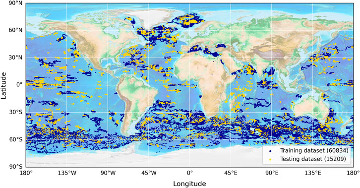
Figure 1. Distribution of the data used in this study, obtained from the global BGC-Argo dataset. A total of 76,043 data points were used, split by time into training (blue) and testing (yellow) datasets for model evaluation. The training dataset begins on 30/05/2010 and ends on 21/04/2022, with the testing dataset continuing on and ending on 27/11/2023.
2.2.2 Satellite data
Global satellite climatology data, at a spatial resolution of 9 km (mapped, level-3 products) and at a temporal resolution of season, were downloaded from NASA’s Ocean Colour data assembly centre (NASA, 2022). The data were collected by the Moderate Resolution Imaging Spectroradiometer (MODIS) sensor on the Aqua satellite. Two products were downloaded, Chl-a concentration (surface) and diffuse attenuation coefficient at 490 nm [converted to the diffuse attenuation coefficient of PAR, following Morel et al. (2007)], for the four seasons.
2.2.3 Mixed-layer depth climatology
Global monthly maps of mixed-layer depth
2.3 Model development
2.3.1 Existing model
Building on the work by Morel and Berthon (1989), Uitz et al. (2006) developed a model through the statistical analysis of 2,419 profiles across the global oceans that estimates
where
2.3.2 New model
The empirical model developed by Uitz et al. (2006) has proven a useful tool for approximating the stock of Chl-a in the euphotic zone from satellite data (e.g., Hatton et al., 2021). However, the model classifies the ocean into binary physical environments, mixed and stratified waters, and further classifies stratified environments into binary trophic levels. In reality, the ocean may not adhere to such a binary classification. Additionally, although based on a two-parameter model (Equation 1), it really requires six parameters to operate over the full range of conditions. Here, building on the approach used by Uitz et al. (2006), we adapt their model to operate continuously over the full range of physical conditions and trophic levels in the ocean while reducing the number of parameters required, thus potentially providing a more parsimonious solution.
We begin by selecting a different but compatible variable to
Next, we model
This model has four parameters,
2.4 Fitting and evaluating models using the global dataset
To tune and test the method used by Uitz et al. (2006) and the new model (Equation 3), the global dataset was split by time (pre- and post-21 April 2022) into a training and testing dataset (∼80–20 split; 60,834–15,209 profiles), both of which were globally representative (Figure 1). We split the data according to time to ensure that the two datasets were independent (Stock and Subramaniam, 2020). Both the method used by Uitz et al. (2006) and the new model (Equation 3) were fitted to the data using the Levenberg–Marquardt least-squares method of minimisation that aims to minimise the chi-squared
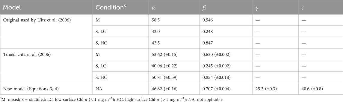
Table 1. Model parameters used and derived in the study. Brackets represent uncertainty in the parameters.
A number of statistical tests were used to evaluate model performance (e.g., Equations 5, 6). This statistical evaluation was completed on both the training and testing datasets. All statistical evaluations were conducted on
where
where
2.5 Application of the new model
To illustrate applications of the new model, we simulated the influence of changes in the mixed-layer depth on model simulations of
3 Results and discussion
3.1 Existing model results
The original model used by Uitz et al. (2006) (see parameters in Table 1) was found to agree well with the BGC-Argo dataset (Figure 2A). There is a clear division between mixed and stratified waters, and the original regressions capture these broad differences (Figure 2A). This division between mixed and stratified waters essentially reflects the fact that within the euphotic zone when waters are mixed, chlorophyll-a is relatively uniform with depth, whereas when conditions stratify, the vertical stricture of chlorophyll-a is non-uniform, with the presence of a DCM. Considering that this model was developed using a much smaller, independent dataset (2,419 profiles) with less extensive global coverage (Uitz et al., 2006), it is quite remarkable how well the original concept developed by Morel and Berthon (1989) performs. The model estimates of
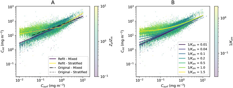
Figure 2. (A) Original model used by Uitz et al. (2006) and the refit of the model used by Uitz et al. (2006) to the global BGC-Argo dataset overlain onto the scatter plot of surface vs column-integrated Chl-a for the entire dataset (training and testing) with points colour-coded according to the ratio
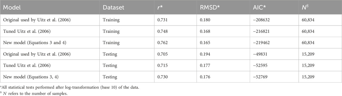
Table 2. Statistical comparison of models with training and testing datasets.
Re-tuning the model used by Uitz et al. (2006) to the training dataset (Table 1) yielded in a significant increase in performance over the original model (lower RMSD and AIC) compared with the testing dataset (Table 2). However, the new set of parameters was only marginally different from the original ones (Figure 2A; Table 1). Regressions for the three different ranges (mixed, stratified low
3.2 New model results
Simulations overlain onto the entire BGC-Argo dataset (training and testing; Figure 2B) illustrate how the new model performs in a continuous manner over the full range of
The
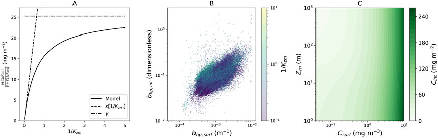
Figure 3. (A) Relationship between the term on the far right-hand side of Equation 3
Compared with the re-tuned and original models used by Uitz et al. (2006), the new model has a similar performance in both the training and testing datasets (Table 2), albeit with a slightly higher correlation coefficient and lower RMSD and AIC. Although these improvements are small, when considering how large the datasets are, improvements are significant, for example, the increase in the correlation coefficient in both training and testing datasets (Table 2, Z-test,
3.3 Changes in vertical structure with increasing stratification
The term on the far right-hand side of Equation 3
To investigate drivers of the right-hand term of Equation 3, we plotted surface particle backscattering
3.4 Model applications
The new model could provide a useful, empirical constraint on future predictions on shifts in the vertical structure of Chl-a in the open ocean in a changing climate. To illustrate this, we simulated (Figure 3C)
Figure 4 shows the seasonal estimates of global
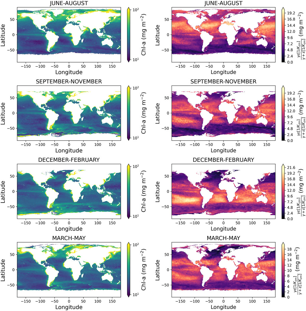
Figure 4. Left column shows global maps of estimated column-integrated Chl-a
Spatial maps of the far right-hand term of Equation 3 (Figure 4) also provide an insight into regions that exhibit strong vertical gradients in Chl-a. The term contributes more significantly in sub-tropical regions but displays temporal variability in seasonal stratified high-latitude regions. Collectively, these images demonstrate how the new model can be used with satellite data and
3.5 Potential limitations to our study and future perspectives
Morel and Berthon (1989) and Uitz et al. (2006) used discrete measurements of extracted Chl-a (either using fluorescence or high-performance liquid chromatography), as opposed to this study that used less accurate in vivo estimates of Chl-a, only available on BGC-Argo floats. For the same Chl-a concentration, variations in the in vivo fluorescence signal can occur with species composition and physiological status, impacting conversion factors (see the study by Petit et al., 2022), especially in the Southern Ocean (Schallenberg et al., 2022). There are also uncertainties in the non-photochemical quenching correction used in BGC-Argo data processing (Schmechtig et al., 2023).
Uncertainties also exist for other variables used in the model. For example, for many profiles, PAR data were not available, so
With the climate changing rapidly, it is important to have tools to provide accurate estimations of the phytoplankton stock and physiology in the global oceans and ensure relevant monitoring of spatial and temporal changes. By developing simple models that can combine the benefits of high-spatial and temporal observation of the surface ocean by satellites, with the vertical profiling of autonomous platforms, we can improve the way we quantify changes in phytoplankton stock and physiology. Moving forward, it will be important to continue tuning the model as more data become available. It may also be fruitful to apply the model to specific regions with unique characteristics where the parameters may differ, for example, in Arctic waters (Ardyna et al., 2013) and the Mediterranean Sea (Li et al., 2022).
3.6 Summary
Using a global array of BGC-Argo floats (76,043 profiles, spanning from 2010 to 2023), we re-evaluated empirical relationships between the surface and column-integrated concentrations of Chl-a developed by Morel and Berthon (1989) and extended by Uitz et al. (2006). We found that these relationships agree well with BGC-Argo float data. The relationships were then extended so that the column-integrated Chl-a concentration could be estimated as a continuous function of its surface value and a proxy for stratification (optical mixed-layer depth) without the need for a binary switch in parameters between mixed and stratified waters. The extended model has fewer parameters and performed better in statistical tests than earlier models. Applications of the new model include studying the impact of increasing stratification on the relationship between surface and column-integrated concentrations of Chl-a, using satellite data for monitoring spatial and temporal variations in column-integrated concentrations of Chl-a, and identifying and monitoring regions of the ocean with strong vertical gradients in Chl-a.
Data availability statement
The original contributions presented in the study are included in the article; further inquiries can be directed to the corresponding author.
Author contributions
ET: formal analysis, funding acquisition, investigation, methodology, resources, software, validation, visualization, and writing–original draft. HE: formal analysis, investigation, visualization, and writing–review and editing. JV: methodology, resources, software, and writing–review and editing. RB: conceptualization, formal analysis, funding acquisition, investigation, methodology, project administration, resources, software, supervision, validation, visualization, writing–original draft, and writing–review and editing.
Funding
The author(s) declare that financial support was received for the research, authorship, and/or publication of this article. RB and JV were funded by a UKRI Future Leader Fellowship (MR/V022792/1). ET was supported by two Engineering and Physical Sciences Research Council summer internships.
Acknowledgments
ET and HE were supported by the B.Sc programme in Environmental Science at the University of Exeter Cornwall. The authors thank all those who contributed to the acquisition and processing of BGC-Argo data. The authors also thank NASA for providing the global MODIS-Aqua data and NOAA for global mixed-layer depths. BGC-Argo data used were collected and made freely available by the International Argo Program and the national programs that contribute to it (https://argo.ucsd.edu, https://www.ocean-ops.org). The Argo Program is part of the Global Ocean Observing System. Satellite data used are freely available on the NASA website (https://oceancolor.gsfc.nasa.gov). Mixed layer depth climatologies used are freely available on the NOAA website (https://www.pmel.noaa.gov/mimoc/). For the purpose of open access, the author has applied a Creative Commons Attribution (CC BY) licence to any Author Accepted Manuscript version arising from this submission.
Conflict of interest
The authors declare that the research was conducted in the absence of any commercial or financial relationships that could be construed as a potential conflict of interest.
The reviewer EC declared a past co-authorship with the author RB to the handling Editor.
Publisher’s note
All claims expressed in this article are solely those of the authors and do not necessarily represent those of their affiliated organizations, or those of the publisher, the editors, and the reviewers. Any product that may be evaluated in this article, or claim that may be made by its manufacturer, is not guaranteed or endorsed by the publisher.
References
Ardyna, M., Babin, M., Gosselin, M., Devred, E., Bélanger, S., Matsuoka, A., et al. (2013). Parameterization of vertical chlorophyll a in the Arctic Ocean: impact of the subsurface chlorophyll maximum on regional, seasonal, and annual primary production estimates. Biogeosciences 10, 4383–4404. doi:10.5194/bg-10-4383-2013
Ardyna, M., Babin, M., Gosselin, M., Devred, E., Rainville, L., and Tremblay, J. (2014). Recent Arctic ocean sea ice loss triggers novel fall phytoplankton blooms. Geophys. Res. Lett. 41, 6207–6212. doi:10.1002/2014GL061047
Ardyna, M., Claustre, H., Sallée, J., D’Ovidio, F., Gentili, B., van Dijken, G., et al. (2017). Delineating environmental control of phytoplankton biomass and phenology in the Southern Ocean. Geophys. Res. Lett. 44, 5016–5024. doi:10.1002/2016GL072428
Barnes, C., Maxwell, D., Reuman, D. C., and Jennings, S. (2010). Global patterns in predator–prey size relationships reveal size dependency of trophic transfer efficiency. Ecology 91, 222–232. doi:10.1890/08-2061.1
Bazzani, E., Lauritano, C., and Saggiomo, M. (2023). Southern Ocean iron limitation of primary production between past knowledge and future projections. J. Mar. Sci. Eng. 11, 272. doi:10.3390/jmse11020272
Behrenfeld, M. J., Boss, E., Siegel, D. A., and Shea, D. M. (2005). Carbon-based ocean productivity and phytoplankton physiology from space. Glob. Biogeochem. Cycles 19. doi:10.1029/2004GB002299
Bittig, H. C., Maurer, T. L., Plant, J. N., Schmechtig, C., Wong, A. P. S., Claustre, H., et al. (2019). A BGC-Argo guide: planning, deployment, data handling and usage. Front. Mar. Sci. 6. doi:10.3389/fmars.2019.00502
Boyd, P., Claustre, H., Levy, M., Siegel, D., and Weber, T. (2019). Multi-faceted particle pumps drive carbon sequestration in the ocean. Nature 568, 327–335. doi:10.1038/s41586-019-1098-2
Brewin, R. J. W., Dall’Olmo, G., Gittings, J., Sun, X., Lange, P. K., Raitsos, D. E., et al. (2022). A conceptual approach to partitioning a vertical profile of phytoplankton biomass into contributions from two communities. J. Geophys. Res. Oceans 127, e2021JC018195. doi:10.1029/2021JC018195
Cael, B., Bisson, K., Boss, E., Dutkiewicz, S., and Henson, S. (2023). Global climate-change trends detected in indicators of ocean ecology. Nature 619, 551–554. doi:10.1038/s41586-023-06321-z
Campbell, J. W. (1995). The lognormal distribution as a model for bio-optical variability in the sea. J. Geophys. Res. Oceans 100, 13237–13254. doi:10.1029/95JC00458
Chai, F., Johnson, K. S., Claustre, H., Xing, X., Wang, Y., Boss, E., et al. (2020). Monitoring ocean biogeochemistry with autonomous platforms. Nat. Rev. Earth and Environ. 1, 315–326. doi:10.1038/s43017-020-0053-y
Cheng, L., Abraham, J., Hausfather, Z., and Trenberth, K. E. (2019). How fast are the oceans warming? Science 363, 128–129. doi:10.1126/science.aav7619
Claustre, H., Johnson, K. S., and Takeshita, Y. (2020). Observing the global ocean with Biogeochemical-Argo. Annu. Rev. Mar. Sci. 12, 23–48. doi:10.1146/annurev-marine-010419-010956
Cornec, M., Claustre, H., Mignot, A., Guidi, L., Lacour, L., Poteau, A., et al. (2021). Deep chlorophyll maxima in the Global Ocean: occurrences, drivers and characteristics. Glob. Biogeochem. Cycles 35, e2020GB006759. doi:10.1029/2020GB006759
Cox, I., Brewin, R. J. W., Dall’Olmo, G., Sheen, K., Sathyendranath, S., Rasse, R., et al. (2023). Distinct habitat and biogeochemical properties of low-oxygen-adapted tropical oceanic phytoplankton. Limnol. Oceanogr. 68, 2022–2039. doi:10.1002/lno.12404
Cullen, J. J. (2015). Subsurface chlorophyll maximum layers: enduring enigma or mystery solved? Annu. Rev. Mar. Sci. 7, 207–239. doi:10.1146/annurev-marine-010213-135111
Dai, Y., Yang, S., Zhao, D., Hu, C., Xu, W., Anderson, D. M., et al. (2023). Coastal phytoplankton blooms expand and intensify in the 21st century. Nature 615, 280–284. doi:10.1038/s41586-023-05760-y
Boyer Montégut, C., Madec, G., Fischer, A. S., Lazar, A., and Iudicone, D. (2004). Mixed layer depth over the global ocean: an examination of profile data and a profile-based climatology. J. Geophys. Res. Oceans 109. doi:10.1029/2004JC002378
Deppeler, S. L., and Davidson, A. T. (2017). Southern Ocean phytoplankton in a changing climate. Front. Mar. Sci. 4. doi:10.3389/fmars.2017.00040
Falkowski, P. G. (1994). The role of phytoplankton photosynthesis in global biogeochemical cycles. Photosynth. Res. 39, 235–258. doi:10.1007/BF00014586
Falkowski, P. G., Laws, E. A., Barber, R. T., and Murray, J. W. (2003). Phytoplankton and their role in primary, new, and export production. Berlin, Heidelberg: Springer Berlin Heidelberg, 99–121. doi:10.1007/978-3-642-55844-3_5
Ferreira, A., Dias, J., Brotas, V., and Brito, A. C. (2022). A perfect storm: an anomalous offshore phytoplankton bloom event in the NE Atlantic (March 2009). Sci. Total Environ. 806, 151253. doi:10.1016/j.scitotenv.2021.151253
Field, C., Behrenfeld, M., Randerson, J., and Falkowski, P. (1998). Primary production of the biosphere: integrating terrestrial and oceanic components. Science 281, 237–240. doi:10.1126/science.281.5374.237
Garnesson, P., Mangin, A., Fanton d’Andon, O., Demaria, J., and Bretagnon, M. (2019). The CMEMS Globcolour chlorophyll a product based on satellite observation: multi-sensor merging and flagging strategies. Ocean Sci. 15, 819–830. doi:10.5194/os-15-819-2019
Gould, J., Sloyan, B., and Visbeck, M. (2013). “Chapter 3 - in situ Ocean Observations: a brief history, present status, and future directions,” in Ocean Circulation and climate - a 21st century perspective (elsevier), 59–81. doi:10.1016/B978-0-12-391851-2.00003-9
Graff, J. R., Westberry, T. K., Milligan, A. J., Brown, M. B., Dall’Olmo, G., van Dongen-Vogels, V., et al. (2015). Analytical phytoplankton carbon measurements spanning diverse ecosystems. Deep Sea Res. Part I Oceanogr. Res. Pap. 102, 16–25. doi:10.1016/j.dsr.2015.04.006
Groom, S., Sathyendranath, S., Ban, Y., Bernard, S., Brewin, R., Brotas, V., et al. (2019). Satellite ocean colour: current status and future perspective. Front. Mar. Sci. 6, 1–30. doi:10.3389/fmars.2019.00485
Hatton, I., Heneghan, R., Bar-On, Y., and Galbraith, E. (2021). The global ocean size-spectrum from bacteria to whales. Sci. Adv. 7, eabh3732. doi:10.1126/sciadv.abh3732
IOCCG (2020). Synergy between ocean colour and biogeochemical/ecosystem models. Tech. Rep in IOCCG report series, No. 19, international ocean colour coordinating group, dartmouth, Canada.
IPCC (2021). Climate change 2021: the physical science basis. Contribution of working group I to the sixth assessment report of the intergovernmental panel on climate change. Cambridge: Cambridge University Press. doi:10.1017/9781009157896
Jayne, S. R., Roemmich, D., Zilberman, N., Riser, S., Johnson, K., Johnson, G., et al. (2017). The argo program: present and future. Oceanography 30, 18–28. doi:10.5670/oceanog.2017.213
Kiørboe, T. (1993). Turbulence, phytoplankton cell size, and the structure of pelagic food webs. Adv. Mar. Biol. (Elsevier) 29, 1–72. doi:10.1016/S0065-2881(08)60129-7
Legendre, L., and Rassoulzadgan, F. (1996). Food-web mediated export of biogenic carbon in oceans: hydrodynamic control. Mar. Ecol. Prog. Ser. 145, 179–193. doi:10.3354/meps145179
Le Moigne, F., Boye, M., Masson, A., Corvaisier, R., Grossteffan, E., Pondaven, P., et al. (2013). Description of the biogeochemical features of the subtropical southeastern Atlantic and the Southern Ocean south of South Africa during the austral summer of the International Polar Year. Biogeosciences 10, 281–295. doi:10.5194/bg-10-281-2013
Le Traon, P.-Y., Antoine, D., Bentamy, B.-H. A., Breivik, L., Chapron, B., Corlett, G., et al. (2015). Use of satellite observations for operational oceanography: recent achievements and future prospects. J. Operational Oceanogr. 8, s12–s27. doi:10.1080/1755876X.2015.1022050
Li, X., Mao, Z., Zheng, H., Zhang, W., Yuan, D., Li, Y., et al. (2022). Process-oriented estimation of chlorophyll-a vertical profile in the Mediterranean Sea using MODIS and oceanographic float products. Front. Mar. Sci. 9. doi:10.3389/fmars.2022.933680
Longhurst, A., Sathyendranath, S., Platt, T., and Caverhill, C. (1995). An estimate of global primary production in the ocean from satellite radiometer data. J. Plankton Res. 17, 1245–1271. doi:10.1093/plankt/17.6.1245
Lu, W., Gao, X., Wu, Z., Wang, T., Lin, S., Xiao, C., et al. (2022). Framework to extract extreme phytoplankton bloom events with remote sensing datasets: a case study. Remote Sens. 14, 3557. doi:10.3390/rs14153557
Ma, L., Bai, X., Laws, E. A., Xiao, W., Guo, C., Liu, X., et al. (2023). Responses of phytoplankton communities to internal waves in oligotrophic oceans. J. Geophys. Res. Oceans 128, e2023JC020201. doi:10.1029/2023jc020201
Marquardt, D. (1963). An algorithm for least-squares estimation of nonlinear parameters. J. Soc. Industrial Appl. Math. 11, 431–441. doi:10.1137/0111030
Martinez-Vicente, V., Dall’Olmo, G., Tarran, G., Boss, E., and Sathyendranath, S. (2013). Optical backscattering is correlated with phytoplankton carbon across the Atlantic Ocean. Geophys. Res. Lett. 40, 1154–1158. doi:10.1002/grl.50252
McClain, F.-G. H. S. C., Feldman, G. C., and Hooker, S. B. (2004). An overview of the SeaWiFS project and strategies for producing a climate research quality global ocean bio-optical time series. Deep Sea Res. Part II Top. Stud. Oceanogr. 51, 5–42. doi:10.1016/j.dsr2.2003.11.001
Mignot, A., Claustre, H., Uitz, J., Poteau, A., D’Ortenzio, F., and Xing, X. (2014). Understanding the seasonal dynamics of phytoplankton biomass and the deep chlorophyll maximum in oligotrophic environments: a bio-argo float investigation. Glob. Biogeochem. Cycles 28, 856–876. doi:10.1002/2013gb004781
Morel, A., and Berthon, J.-F. (1989). Surface pigments, algal biomass profiles, and potential production of the euphotic layer: relationships reinvestigated in view of remote-sensing applications. Limnol. Oceanogr. 34, 1545–1562. doi:10.4319/lo.1989.34.8.1545
Morel, A., Huot, Y., Gentili, B., Werdell, P., Hooker, S., and Franz, B. (2007). Examining the consistency of products derived from various ocean color sensors in open ocean (case 1) waters in the perspective of a multi-sensor approach. Remote Sens. Environ. 111, 69–88. doi:10.1016/j.rse.2007.03.012
NASA (2022). NASA goddard space flight center, ocean ecology laboratory, ocean biology processing group in Moderate-resolution imaging spectroradiometer (MODIS) Aqua CHL data. Greenbelt: NASA OB.DAAC. doi:10.5067/AQUA/MODIS/L3M/CHL/2022
Nowicki, M., DeVries, T., and Siegel, D. (2022). Quantifying the carbon export and sequestration pathways of the ocean’s biological carbon pump. Glob. Biogeochem. Cycles 36, e2021GB007083. doi:10.1029/2021gb007083
Oka, R., Talley, L., and Suga, T. (2007). Temporal variability of winter mixed layer in the mid-to high-latitude North Pacific. J. Oceanogr. 63, 293–307. doi:10.1007/s10872-007-0029-2
Petit, F., Uitz, J., Schmechtig, C., Dimier, C., Ras, J., Poteau, A., et al. (2022). Influence of the phytoplankton community composition on the in situ fluorescence signal: implication for an improved estimation of the chlorophyll-a concentration from biogeochemical-argo profiling floats. Front. Mar. Sci. 9. doi:10.3389/fmars.2022.959131
Roemmich, D., Johnson, G., Riser, S., Davis, R., Gilson, J., Owens, W., et al. (2009). The argo program: observing the global oceans with profiling floats. Oceanography 22, 34–43. doi:10.5670/oceanog.2009.36
Schallenberg, C., Strzepek, R. F., Bestley, S., Wojtasiewicz, B., and Trull, T. W. (2022). Iron limitation drives the globally extreme fluorescence/chlorophyll ratios of the Southern Ocean. Geophys. Res. Lett. 49, e2021GL097616. doi:10.1029/2021GL097616
Schmechtig, C., Claustre, H., Poteau, A., D’Ortenzio, F., Schallenberg, C., Trull, T., et al. (2023). BGC-Argo quality control manual for the Chlorophyll-a concentration. doi:10.13155/35385
Schmidtko, S., Johnson, G. C., and Lyman, J. M. (2013). MIMOC: a global monthly isopycnal upper-ocean climatology with mixed layers. J. Geophys. Res. Oceans 118, 1658–1672. doi:10.1002/jgrc.20122
Sergi, S., Baudena, A., Cotte, C., Ardyna, M., Blain, S., and d’Ovidio, F. (2020). Interaction of the Antarctic circumpolar current with seamounts fuels moderate blooms but vast foraging grounds for multiple marine predators. Front. Mar. Sci. 7. doi:10.3389/fmars.2020.00416
Sridevi, B., Srinivasu, K., Bhavani, T., and Prasad, K. (2019). Extreme events enhance phytoplankton bloom in the south-western Bay of Bengal. Indian J. Geo Mar. Sci. 48, 253–258.
Stock, A., and Subramaniam, A. (2020). Accuracy of empirical satellite algorithms for mapping phytoplankton diagnostic pigments in the open ocean: a supervised learning perspective. Front. Mar. Sci. 7. doi:10.3389/fmars.2020.00599
Strzedek, R., Boyd, P., and Sunda, W. (2019). Photosynthetic adaptation to low iron, light, and temperature in Southern Ocean phytoplankton. Proc. Natl. Acad. Sci. 116, 4388–4393. doi:10.1073/pnas.1810886116
Trainer, V., Moore, S., Hallegraeff, G., Kudela, R., Clement, A., Mardones, J., et al. (2020). Pelagic harmful algal blooms and climate change: lessons from nature’s experiments with extremes. Harmful Algae 91, 101591. doi:10.1016/j.hal.2019.03.009
Uitz, J., Claustre, H., Morel, A., and Hooker, S. (2006). Vertical distribution of phytoplankton communities in open ocean: an assessment based on surface chlorophyll. J. Geophys. Res. Oceans 111. doi:10.1029/2005jc003207
Viljoen, J. V., Sun, X., and Brewin, R. J. W. (2024). Climate variability shifts the vertical structure of phytoplankton in the Sargasso Sea. Nat. Clim. Change. doi:10.1038/s41558-024-02136-6
Wang, Y., Chen, H.-H., Tang, R., He, D., Lee, Z., Xue, H., et al. (2022). Australian fire nourishes ocean phytoplankton bloom. Sci. Total Environ. 807, 150775. doi:10.1016/j.scitotenv.2021.150775
Wang, Y., Liu, D., Xiao, W., Zhou, P., Tian, C., Zhang, C., et al. (2021). Coastal eutrophication in China: trend, sources, and ecological effects. Harmful Algae 107, 102058. doi:10.1016/j.hal.2021.102058
Keywords: phytoplankton, BGC-Argo, vertical structure, global, ocean colour, chlorophyll-a
Citation: Tanner EP, Ewin H, Viljoen JJ and Brewin RJW (2024) Revisiting the relationship between surface and column-integrated chlorophyll-a concentrations in the Biogeochemical-Argo and satellite era. Front. Remote Sens. 5:1495958. doi: 10.3389/frsen.2024.1495958
Received: 13 September 2024; Accepted: 25 November 2024;
Published: 11 December 2024.
Edited by:
Vittorio Ernesto Brando, National Research Council (CNR), ItalyCopyright © 2024 Tanner, Ewin, Viljoen and Brewin. This is an open-access article distributed under the terms of the Creative Commons Attribution License (CC BY). The use, distribution or reproduction in other forums is permitted, provided the original author(s) and the copyright owner(s) are credited and that the original publication in this journal is cited, in accordance with accepted academic practice. No use, distribution or reproduction is permitted which does not comply with these terms.
*Correspondence: Robert J. W. Brewin, ci5icmV3aW5AZXhldGVyLmFjLnVr