Landcover-specific calibration of the optical trapezoid model (OPTRAM) for soil moisture monitoring in the Central Valley, California

The Optical TRApezoid Model (OPTRAM) has been extensively utilized to map high-resolution surface soil moisture (top 0–5 cm) using surface reflectance observations. OPTRAM parameters, the intercept and slope of the dry and wet edges, are typically calibrated by analyzing the data cloud created from the Normalized Difference Vegetation Index (NDVI) and the Shortwave-infrared Transformed Reflectance (STR) in a specified area of interest. One set of parameters is commonly obtained for the entire study area regardless of its soil and landcover types. In this study, we explored to what extent a landcover-specific calibration of OPTRAM can improve its accuracy. In this analysis, we used Sentinel-2 (S2) reflectance and the Cropland Data Layer (CDL) landcover datasets via the Google Earth Engine to generate 20-m resolution soil moisture maps for California’s Central Valley (CV). We evaluated the spatial and temporal accuracy of the CV-wide calibrated OPTRAM (OPTRAM-CV) and landcover-specific calibrated OPTRAM (OPTRAM-LS) against in situ observations and SMAP-HydroBlocks (SMAP-HB), a well-validated 30-m satellite-based soil moisture dataset. Our results indicate that OPTRAM-LS significantly improved the accuracy of soil moisture estimates compared to OPTRAM-CV. The average root mean square error was 0.09 and 0.05 (m³ m⁻³) for OPTRAM-CV and OPTRAM-LS, respectively. OPTRAM showed less accuracy than SMAP-HB compared to in situ observations but yielded higher resolution than SMAP-HB.

1 Introduction

Soil moisture is an important environmental factor influencing the water, carbon, and energy exchange at the surface-atmosphere interface (Robinson et al., 2008; De Queiroz et al., 2020). This variable plays a key role in hydrology by shaping rainfall-runoff processes, impacting ecology by regulating net ecosystem exchange (Ochsner et al., 2013; Hosseini et al., 2023), and affecting agriculture by influencing the plant water availability, plant productivity and crop yields (Wang et al., 2011). Moreover, soil moisture is effective in monitoring drought conditions (Vergopolan et al., 2021a; b; Wang et al., 2019) and wildfire occurrence and severity (Jensen et al., 2018). This led to an increased focus on monitoring spatially distributed soil moisture data at large scales and on a timely basis using remotely sensed images (Ahmed et al., 2011; Huete, 2004).

Microwave remote sensing techniques demonstrate great potential due to their ability to penetrate through both vegetation canopy and the underlying soil, particularly at lower frequencies (Entekhabi et al., 2010). Satellites such as Soil Moisture Active Passive (SMAP) and Soil Moisture and Ocean Salinity (SMOS) have shown good promise for global mapping of near-surface (0–5 cm) soil moisture at a spatial resolution of 25–40 km and temporal resolution of 2–3 days (Mohanty et al., 2017). However, this spatial resolution is too coarse for many agriculture, hydrology, and water resources applications. Hence, optical and thermal satellite observations are frequently employed to bridge the scale gap due to their higher spatial resolutions (Sadeghi et al., 2017).

Over the past few years, the Optical TRApezoid Model (OPTRAM) (Sadeghi et al., 2017) has been utilized to map soil moisture using optical reflectance observations. This model was established based on research by Sadeghi et al. (2015), which derived a linear, physically-based relationship between soil moisture and Shortwave Infrared (SWIR) Transformed Reflectance (STR). Assuming a linear correlation between soil and vegetation water contents, OPTRAM assumes that the Normalized Difference Vegetation Index (NDVI) and STR data form a trapezoidal data cloud where drier pixels are generally located at a lower position than wetter pixels. In OPTRAM, two lines are fitted to the bottom and top edges of the dense part of the data cloud, referred to as the dry and wet edges. Then, each pixel’s soil moisture value is assigned based on its distance from the dry and wet edges of the data cloud.

Although OPTRAM has demonstrated promising results for high-resolution mapping of soil moisture (Ambrosone et al., 2020; Chen et al., 2020; Pandey et al., 2024; Mananze et al., 2019; Burdun et al., 2020; Mokhtari et al., 2023), some users have reported challenges in determining the dry and wet edge parameters (Sadeghi et al., 2023). This problem is more pronounced in diverse regions with distinct values of STR and NDVI associated with various landcover types. Such limitations stem from the variability in reflectance properties across different features and landcover types (Huete, 2004; Mohamadzadeh and Ahmadisharaf, 2024; Shu et al., 2024). Therefore, the current practice, wherein a single set of model parameters is used for the entire region of interest, does not accurately represent the true characteristics of the region. This approach introduces bias, reflecting the values of the predominant landcover type that forms the majority of the cloud. Consequently, ignoring the landcover type in the data cloud formation negatively affects the OPTRAM parameters, thereby imposing a constraint on the OPTRAM methodology.

To address this issue, we explore to what extent a landcover-specific calibration of OPTRAM improves its accuracy. In the following sections, we provide an overview of the theoretical basis of OPTRAM, discuss how the different spectral reflectance of various landcover types justifies the importance of a landcover-specific calibration, and present a comparative analysis of the landcover-specific calibrated OPTRAM.

2 Theoretical background

Sadeghi et al. (2017) derived OPTRAM based on the physical relationship between surface soil moisture and SWIR reflectance. OPTRAM calculates soil moisture θ as:

$\theta ={\theta }_d+\left({\theta }_w-{\theta }_d\right)\frac{\text{STR}-{\text{STR}}_d}{{\text{STR}}_w-{\text{STR}}_d}(1)$

where STR represents the SWIR transformed reflectance, and STR_d and STR_w are STR at the dry edge (θ = θ_d) and wet edge (θ = θ_w), respectively. The relationship between STR and SWIR reflectance, R_SWIR, is expressed as follows (Sadeghi et al., 2015):

$STR=\frac{{\left(1-R_{SWIR}\right)}^2}{2R_{SWIR}}(2)$

Assuming a linear correlation between soil and vegetation water content, it is anticipated that the NDVI and STR will form a trapezoidal data cloud, where drier pixels are located at a lower position and wetter pixels are located at a higher position on the data cloud. Fitting two lines to the lower and upper edges of the densest part of the data cloud, the dry and wet edges are formulated as follows:

${\text{STR}}_d=i_d+s_d\text{NDVI}(3)$

${\text{STR}}_w=i_w+s_w\text{NDVI}(4)$

where i_d and s_d are the intercept and the slope of the dry edge, respectively, and i_w and s_w are the intercept and slope of the wet edge, respectively.

Accordingly, OPTRAM assigns a soil moisture value to each pixel, considering its proximity to the dry and wet edges of the data cloud. By combining Equations 1–4 and assuming θ_d = 0 and θ_w = θ_s, where θ_s is the soil porosity, soil moisture for each pixel can be estimated as a function of STR and NDVI as follows:

$\theta ={\theta }_s\left[\frac{i_d+s_d\text{NDVI}-\text{STR}}{i_d-i_w+\left(s_d-s_w\right)\text{NDVI}}\right](5)$

Considering Equations 3, 4, OPTRAM assumes that pixels with identical NDVI values yield identical STR_d and STR_w values, regardless of the vegetation type. However, the new approach acknowledges that OPTRAM parameters (i_d, s_d, i_w, s_w) are not constant over the study area because STR_d and STR_w can vary not only with NDVI but also with vegetation type. This leads to diverse OPTRAM parameters at a constant NDVI for various landcover types.

It is intuitively understandable that two different vegetation types might have the same greenness at a certain vegetation density. However, they can still have substantially different reflectance due to their distinct canopy structure. This variability implies that s_d and s_w may significantly vary with landcover types.

This landcover-specific variability is also the case for NDVI = 0, where soil reflectance may vary not only with soil moisture but also with soil texture and roughness (Huete, 2004). Here, we assume that distinct landcover types most likely contain distinct soil types as well. That is why different landcover types often show substantially different soil reflectance when bare. Consequently, we propose different i_d and i_w values for different landcover types, assuming they contain different soil types.

3 Materials and methods

3.1 Datasets

This study focused on California’s Central Valley (CV), widely known as an agricultural hub, producing nearly 80 crops such as almonds, cotton, grapes, alfalfa, lettuce, walnuts, and tomatoes (Sleeter, 2008). Beyond its agricultural significance, the CV accommodated nearly 7 million residents by 2010 (Soulard and Wilson, 2015). With a diverse mosaic of agricultural and urban landcover types, we considered this region an appropriate test case for exploring the effects of landcover variability on OPTRAM performance. The following datasets were used in this analysis.

3.1.1 Sentinel-2

For the input variables NDVI and STR in Equation 5, we used Multispectral ESA Sentinel-2 (S2) satellite to benefit from its high spatial resolution (10 m for visible, 20 m for SWIR) and temporal resolution (5–10 days) (Wang and Atkinson, 2018). We applied atmospheric correction to ensure accurate surface reflectance and used cloud-free S2 images acquired between 2015 and 2019. Clouds were masked using the Quality Assessment (QA) band to generate a precise bitmask. Observations at the red band (S2 band 4, 665 nm) and NIR band (S2 band 8, 842 nm) were used to calculate NDVI, $\left(NIR-red\right)/\left(NIR+red\right)$, and the SWIR band (S2 band 12, 2190 nm) was used to calculate STR (Equation 2).

3.1.2 SMAP-HB

To evaluate OPTRAM’s performance, we initially considered in situ soil moisture measurements. However, the scarcity of available data in the CV substantially limited our ability to calibrate and validate OPTRAM. Moreover, stations may not be located at the actual irrigation points within croplands, leading to potential discrepancies between soil moisture measurements and vegetation response, introducing uncertainties in the spatial analysis. To address this challenge, we used the SMAP-HB soil moisture dataset, which is well-validated using extensive in situ observation in the US (Vergopolan et al., 2020; Vergopolan et al., 2021a; Vergopolan et al., 2021b). SMAP-HB maps soil moisture at 30-m spatial resolution by integrating original SMAP data, land surface model simulations, and in situ soil moisture observations. SMAP-HB spatial coverage over the CV enabled us to calibrate our models for any part of the area.

3.1.3 Cropland Data Layer (CDL)

To obtain landcover information, we utilized the Cropland Data Layer (CDL) dataset, generated annually for the continental United States. This dataset was created based on satellite observation and extensive agricultural ground truth data (Boryan et al., 2011). Figure 1 shows the CDL landcover classification over the CV used in this study. According to this classification, CV encompasses over 20 distinct landcover types, with 12 predominant ones covering approximately 80 percent of the area.

Figure 1

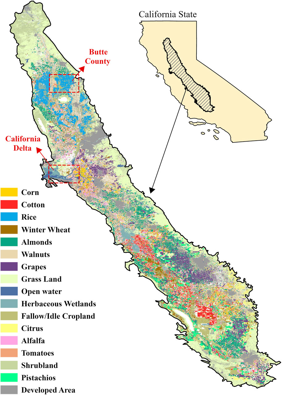
Figure 1. Central Valley landcover map based on the Cropland Data Layer (CDL) dataset. Red rectangles mark the locations of Butte County and the California delta, which are used to compare the spatial resolution of soil moisture maps retrieved from OPTRAM-LS to SMAP-HB (reference) in Figure 6.

3.1.4 In situ soil moisture data

For further validation of OPTRAM, we used in situ soil moisture data from the AmeriFlux and National Oceanic and Atmospheric Administration (NOAA, 2024) networks. Given California’s sparse soil moisture network, we incorporated stations from across the state rather than focusing solely on the CV for validation. Soil moisture data are available for only 16 out of 35 AmeriFlux stations in California. Although data availability varied across these sites, spanning from 2001 to 2022, our analysis was focused on the period covered by the SMAP-HB data period (2015–2019). Consequently, we excluded specific sites with temporal coverage outside this timeframe, e.g., the US-Snd site, which had data available only from 2007 to 2014 (Goulden, 2018). Similarly, stations with a temporal coverage of less than 24 months, such as US-CZ2 and US-CZ3, were not considered (Goulden, 2018). As a result, our acquisition of AmeriFlux soil water content data led to a narrowed dataset consisting of 4 sites, namely, US-Bi1 (Bouldin Island Alfalfa), US-Snf (Sherman Barn), US-Ton (Tonzi Ranch), US-Var (Vaira Ranch- Ione).

The NOAA (2024) network comprises sensors installed at varying depths, ranging from 5 to 100 cm, across California. These sensors cover different periods, spanning from 2005 to 2023. NOAA (2024) sites providing soil moisture data in California are namely as follows; bve (Bridgeville), czc (Cazadero), hbg (Healdsburg), hbk (Hornbrook), hld (Hopland), lsn (Lake Sonoma), mdt (Middletown), ptv (Potter Valley), pvc (Potter Valley Central), pvw (Potter Valley West), rod (Rio Nido), rve (Redwood Valley East), rvn (Redwood Valley North), rvw (Redwood Valley West), str (Santa Rosa), and wls (Willits). We preferably used 5-cm data to evaluate OPTRAM-based soil moisture estimates. In cases where this depth was unavailable (e.g., bve and hbg sites), 10-cm data were used in our analysis.

3.2 Data analysis

We coded Equation 5 in the Google Earth Engine (GEE) platform, where S2 and CDL data were already available. We also uploaded monthly-averaged SMAP-HB data to GEE. OPTRAM parameters (i_d, s_d, i_w, and s_w) were obtained by least-square fitting of Equation 5 to S2 NDVI and STR and SMAP-HB soil moisture data. We obtained one set of parameters for the entire CV for evaluating a CV-wide calibrated OPTRAM (OPTRAM-CV) and one for each landcover type for exploring a landcover-specific calibrated OPTRAM (OPTRAM-LS).

Using these calibrated parameters, moisture content was estimated for both OPTRAM-CV and OPTRAM-LS approaches at the original 10-m resolution for each image in the S-2 collection. However, to derive the monthly mean values, we needed to account for multiple images per month, covering billions of 10-m pixels across the CV. Due to the computational limit of GEE for free accounts, aggregating high-resolution soil moisture estimates at a monthly scale was not feasible. To resolve this issue, we computed the monthly mean soil moisture values by applying a mean reducer at a 30-m scale over the region. The resulting soil moisture estimates were validated using in situ and SMAP-HB data.

4 Results and discussion

Figure 2 compares SMAP-HB high-resolution soil moisture data against available in situ observations in California. As observed, SMAP-HB is well correlated with in situ observations, with a mean R² of 0.6 and an RMSE of 0.08 m³ m^-3, which is larger than the community- accepted level of error (0.04 m³ m⁻³). The observed deviations could be due to uncertainties in the SMAP-HB inputs such as topography, land cover, soil properties, and meteorological data, the lack of representation of human activities, such as irrigation, reservoir operation, groundwater pumping, and several other reasons discussed by Vergopolan et al. (2020), Vergopolan et al. (2021a); Vergopolan et al. (2021b). Nonetheless, SMAP-HB captures the temporal dynamics of soil moisture at individual sites well (shown later). This made us confident in using SMAP-HB as a reliable high-resolution soil moisture dataset for evaluating OPTRAM in California.

Figure 2

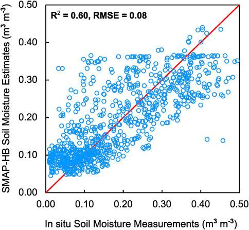
Figure 2. SMAP-HB soil moisture estimates compared to in situ soil moisture data from the NOAA (2024) and AmeriFlux Networks, 2015–2019.

Table 1 lists the calibrated parameters for OPTRAM-CV (entire CV) and OPTRAM-LS (individual landcover types). As seen, the dry and wet edges for the entire CV are largely distant from each other, mainly due to the high spatial variability of STR over the CV (e.g., high STR values in oversaturated rice fields versus low STR values in dry zones of the CV). However, the landcover-specific edges are much closer in most landcover types. While the dry edge shows a marginal variability, the wet edge varies significantly in different landcover classes. To better visualize this variability, Figure 3 shows the STR-NDVI trapezoidal space in three example CV areas, including rice fields, grasslands, and the entire CV. As observed, the trapezoidal space is substantially different for different areas. This emphasizes the importance of a landcover-specific calibration of OPTRAM, as proposed here, and the extent to which one might expect different results from OPTRAM-CV and OPTRAM-LS. For example, satellite observation of STR = 5 in a grassland over the CV would be interpreted as nearly dry soil moisture by OPTRAM-CV but near-saturated soil moisture by OPTRAM-LS (see the first row of Figure 4).

Table 1

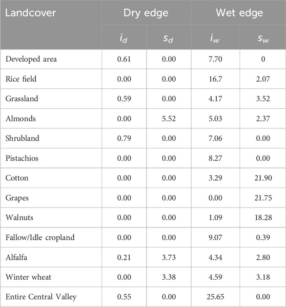
Table 1. OPTRAM calibrated parameters for various landcover types in the Central Valley, California.

Figure 3

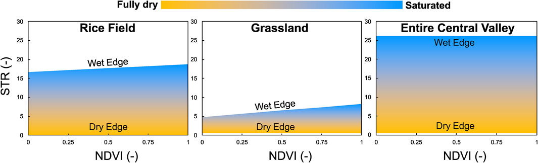
Figure 3. Variability of OPTRAM parameters (dry and wet edges) in three example areas of the Central Valley: rice fields, grasslands, and the entire Central Valley.

Figure 4

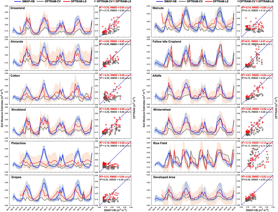
Figure 4. Soil moisture estimates by SMAP-HB (reference), OPTRAM-CV and OPTRAM-LS from 2015 to 2019 for various landcover types over the Central Valley, California. The solid lines represent the monthly mean values, and the shaded areas indicate the variability in estimates.

Figure 4 presents the OPTRAM-CV and OPTRAM-LS soil moisture estimates compared to SMAP-HB as a reference. As observed, OPTRAM-LS is significantly more accurate than OPTRAM-CV. Across all landcover types, the root mean square error (RMSE) is notably lower in OPTRAM-LS. For instance, in grassland, a major landcover constituting over 20 percent of the CV, and in winter wheat, another prevalent landcover type in the CV, OPTRAM-LS brings the RMSE close to the community-accepted level of error (0.04 m³ m⁻³), while the error in OPTRAM-CV is more than twice this level (0.09 m³ m⁻³). Except for rice fields, walnuts, and pistachios, OPTRAM-LS provides reasonable soil moisture estimates, with about 0.04–0.06 (m³ m^-3) deviations from SMAP-HB.

Figure 4 also indicates a generally higher correlation (in terms of R²) between OPTRAM-LS and SMAP-HB than between OPTRAM-CV and SMAP-HB. This enhanced correlation is evident across most landcover types, including almonds, cotton, grapes, fallow idle cropland, alfalfa, winter wheat, and rice fields. It is important to note that OPTRAM with CV-wide calibrated parameters shows an almost zero correlation with SMAP-HB in cotton and grape landcovers, which constitute a small portion of the CV. However, a meaningful correlation appears when this model is calibrated specifically for these landcovers. This emphasizes the nonlinear nature of OPTRAM, Equation 5, where different sets of model parameters do not necessarily yield linearly correlated soil moisture outputs. That said, there are other landcover types where changing the model parameters led to a linear change in the OPTRAM soil moisture estimates, resulting in the same R² between OPTRAM and SMAP-HB (e.g., shrublands and developed areas). Nonetheless, OPTRAM-LS decreased the bias in these landcovers, as shown by the decreased RMSEs. Figure 4 indicates that, despite the significant improvement of OPTRAM through the landcover-specific calibration, it still shows relatively large deviations from SMAP-HB in some landcover types. This deviation is largely due to the much simpler nature of OPTRAM compared to SMAP-HB, as the former tries to estimate soil moisture solely from optical images, while the latter integrates SMAP brightness temperature and physically modeled soil moisture, which uses meteorological data, soil properties, topography, and land cover as input.

The largest deviation between OPTRAM and SMAP-HB is in rice fields. This deviation, however, could be due to not only OPTRAM errors but also SMAP-HB errors. As observed, SMAP-HB shows only one soil moisture peak in the wet season, while OPTRAM exhibits two peaks, one in the wet season and another in April and May. The OPTRAM time series is closer to our expectations for rice fields in California. Farmers in Butte, Glenn, Colusa, Sutter, and Yuba counties often start to saturate their fields with flood irrigation at the beginning of May and drain around the beginning of September. Winter flooded decomposition in many rice fields brings another soil moisture peak. The timing and locations of winter flooded decomposition may vary yearly depending on weather and farming practices. As seen in Figure 5, OPTRAM captured the distribution of winter flooded decomposition in these counties in January and November 2018. Although SMAP-HB has limitations in representing the high-resolution spatial distribution of human-managed processes (e.g., irrigation, reservoir water release), it captures part of the effect through lower-resolution SMAP soil data. That is why SMAP-HB showed some increase in soil moisture in rice fields around May but not full soil saturation. OPTRAM, however, captured the full soil saturation because it could be clearly seen in the S2 SWIR images.

Figure 5

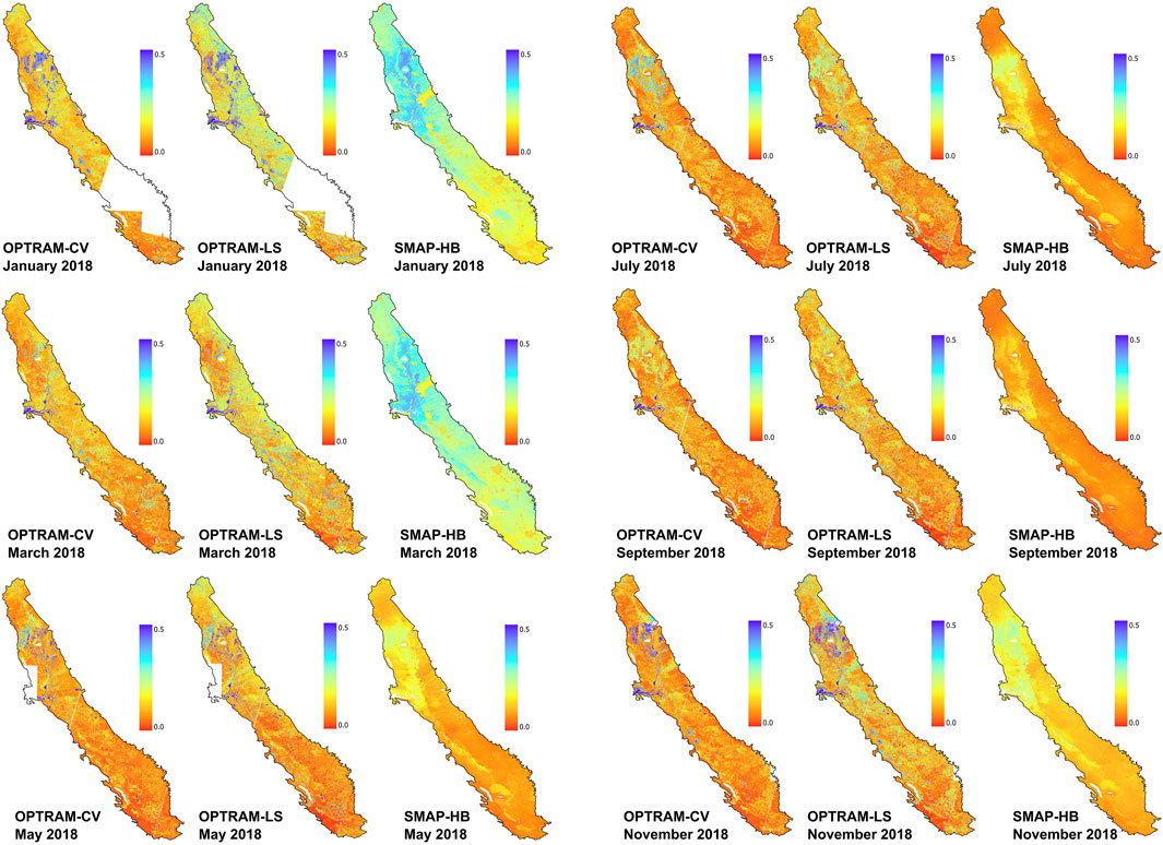
Figure 5. The spatial distribution of monthly OPTRAM, OPTRAM-LS, and SMAP-HB retrievals of surface soil moisture (m³ m^-3) over Central Valley, California, in January, March, and May 2018.

Figure 5 presents sample soil moisture maps in the CV based on OPTRAM and SMAP-HB. As observed, significantly different spatial distributions are shown by these two models. The most notable observation from this figure is that SMAP-HB soil moisture is much smoother than that of OPTRAM. By integrating higher spatial resolution satellite observations, OPTRAM could better capture the fine-scale variabilities between agricultural fields than SMAP-HB. Although both methods have a nominal spatial resolution of 30 m, SMAP-HB’s capability to capture such fine-scale differences is hampered by the SMAP satellite’s large-scale footprint. It yields a narrow range of soil moisture for large clusters, where a high spatial variability is generally expected due to land surface heterogeneity (see Figure 1).

The contrast in spatial resolution is more clearly highlighted when comparing soil moisture maps from May, especially in the Sacramento-San Joaquin Delta and rice fields of northern California. OPTRAM detects many saturated and oversaturated pixels in these areas, which are common due to abundant surface water. As mentioned earlier, the high soil moisture values in rice fields are due to flood irrigation, a common practice in California from May to August. In contrast, SMAP-HB shows a smooth mid-level soil moisture for the entire area with no saturated pixels. This observation agrees with the patterns shown in Figure 4, where SMAP-HB presents only one soil moisture peak in the wet season, but OPTRAM exhibits one more soil moisture peak in May.

To better illustrate this, Figure 6 shows additional sample soil moisture maps over the Delta area and some rice fields within Butte County (see Figure 1). The true-color images of these areas are also included, which shed light on the expected actual spatial resolution of soil moisture. As observed, the spatial variability of OPTRAM is well aligned with the true-color image. All the individual fields, surface water pathways, and permanent water bodies are clearly seen in OPTRAM but are barely distinguishable in SMAP-HB. This demonstrates that OPTRAM is more accurate in capturing the spatial variability of soil moisture.

Figure 6

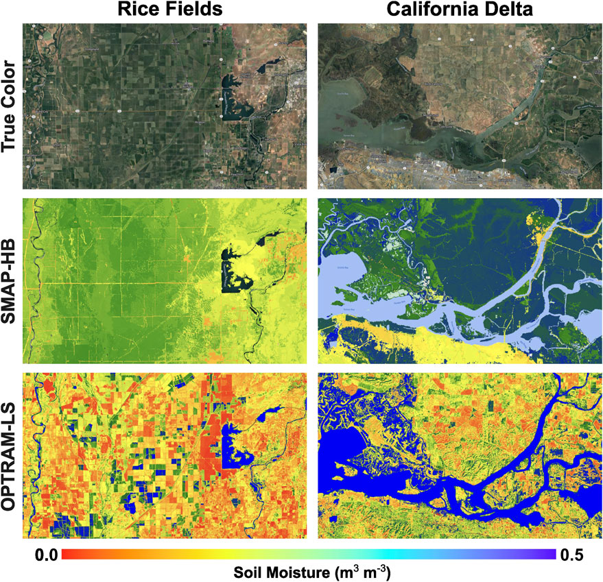
Figure 6. True-color image, SMAP-HB and OPTRAM-LS retrieval of surface soil moisture over the rice fields of Butte County (May 2019) and the California Delta (February 2019). Locations are indicated in Figure 1.

Another observation in Figure 5 is that OPTRAM-CV is generally biased toward drier soil moisture values compared to SMAP-HB. As expected, OPTRAM-LS reduces this bias because it was calibrated for each landcover class directly based on SMAP-HB data. Figure 7 takes a closer look at the dry bias in OPTRAM-CV in some sample areas, including grape vineyards within Fresno and Madera counties (January 2019), grasslands within Tehama County (April 2019), and shrublands in the northern CV (April 2019). As observed, OPTRAM-LS and SMAP-HB consistently estimate wetter soils than OPTRAM-CV in these areas. This dry bias in OPTRAM-CV can be explained by the model parameters, which are not representative when averaged out for the entire CV. As shown in Figure 3, the CV-wide calibration of OPTRAM leads to a much higher wet edge than expected for most landcovers, causing the observed dry bias. Figure 7 emphasizes the importance of a landcover-specific calibration of OPTRAM to achieve reasonable soil moisture maps based on this optical remote sensing approach.

Figure 7

Figure 7. OPTRAM, OPTRAM-LS and SMAP-HB estimates of surface soil moisture for some sample landcovers within the Central Valley, including grapes in January 2019 and grassland and shrubland in April 2019.

In Figure 8, remotely sensed soil moisture values from SMAP-HB, OPTRAM, and OPTRAM-LS are compared with in situ soil moisture measurements from the NOAA (2024) and AmeriFlux Networks. As observed, SMAP-HB estimations exhibit a high correlation with soil moisture measurements in all sites, with an R² greater than 0.8. Furthermore, its RMSE ranges between 0.04 and 0.09 m³ m⁻³, which is higher than community accepted error (0.04 m³ m⁻³) (Entekhabi et al., 2014). As the source of these errors have been discussed earlier, SMAP-HB remains a reliable high-resolution soil moisture dataset.

Figure 8

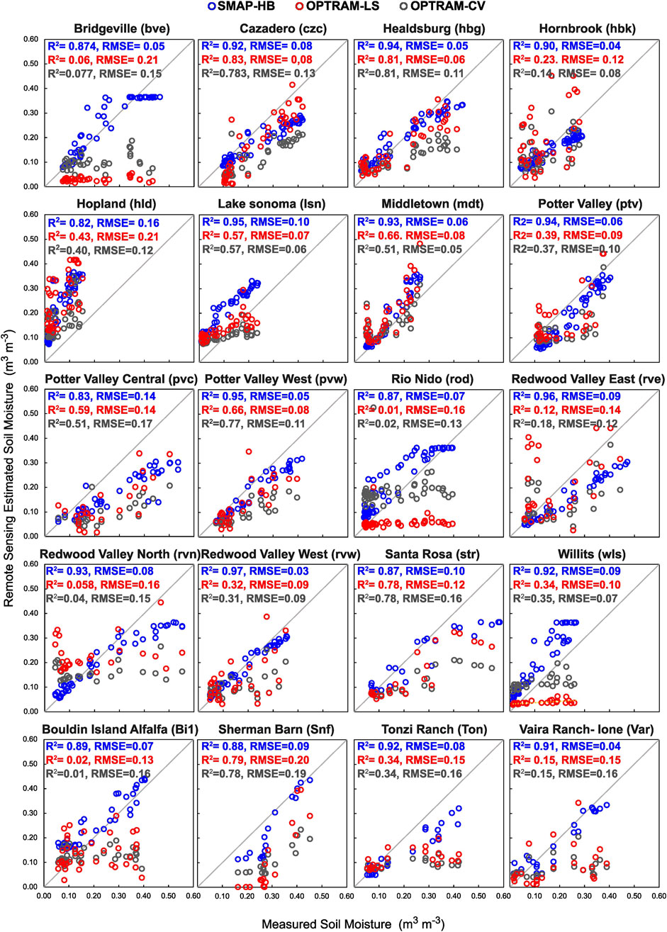
Figure 8. Remote sensing estimated soil moisture (SMAP-HB, OPTRAM-LS, OPTRAM-CV) compared to in situ soil moisture data from the NOAA (2024) and AmeriFlux Networks.

The comparison between OPTRAM-CV and OPTRAM-LS to the soil moisture measurements shows that in some sites, namely czc, hbg, and pvc, OPTRAM-LS outperforms OPTRAM-CV by exhibiting a higher correlation with in situ measurements as well as a lower RMSE. However, at some other sites, namely bve, rod, rve, and wls, OPTRAM-CV performs better than OPTRAM-LS. In general, the difference between OPTRAM-CV and OPTRAM-LS is marginal in this case. This is mainly because OPTRAM generally shows poor correlations with in situ data. This reflects that only drastic soil moisture changes and large-scale patterns can be seen in the optical images, while many local variations, such as irrigation effects on soil moisture, remain hidden in the optical images. Accordingly, OPTRAM is expected to work beyond a certain spatial resolution and fails at very high resolutions, where many other variables than soil moisture (roughness, canopy structure, lighting, image quality, etc.) can change the optical reflectance.

The higher SMAP-HB performance, in this case, suggests that OPTRAM’s performance can be improved by feeding it with other independent variables than just optical reflectance data (e.g., precipitation, low-resolution SMAP soil moisture, etc.) or by applying techniques to minimize noise in the optical reflectance data caused by non-soil moisture variations such as canopy dynamics, cloud cover, and shadows.

5 Conclusion

In this paper, we examined the possibility of using Sentinel-2 optical reflectance data to map soil moisture in California’s Central Valley (CV) via the OPTRAM approach. We initially calibrated OPTRAM for the entire CV (OPTRAM-CV) and then studied the extent to which a landcover-specific calibration (OPTRAM-LS) can improve the general performance of this model. We used the well-validated SMAP-HB dataset as a reference in our evaluations.

One major finding of this study is that the landcover-specific calibration could significantly improve OPTRAM performance over the CV, owing to the fact that CV is a vast area with a diverse array of landcover types. In general, OPTRAM-CV showed a dry bias compared to SMAP-HB, whereas OPTRAM-LS narrowed down this bias. This error is due to the CV-wide calibrated parameters, which were not representative of individual landcover types. In particular, the CV-wide calibration led to a much higher wet edge than expected for most landcovers, which caused the dry bias.

Another major finding of this study is the importance of optical remote sensing in producing high-resolution soil moisture data. SMAP-HB was shown to be a reliable and accurate dataset in terms of the temporal dynamics (seasonality and inter-annual variability) of soil moisture. However, the coarse SMAP resolution (36 km resampled to 10 km) hinders SMAP-HB’s capability to capture local-scale irrigation and diverse crop types. In contrast, OPTRAM explicitly accounts for these variables through Sentinel-2 high-resolution images. Hence, while SMAP-HB provides a sophisticated and more accurate approach for soil moisture estimates every 2–3 days, OPTRAM can be considered a less demanding and more spatially representative alternative for monthly scale soil moisture variations.

Higher SMAP-HB accuracy in this study suggests further research to increase OPTRAM performance by accepting other independent variables, such as precipitation or SMAP soil moisture. How to integrate these additional variables into OPTRAM’s semi-analytical formulation remains a question for future research. In addition, more specified OPTRAM calibration strategies, for example, for individual soil textures, can be studied to further improve its accuracy.

Data availability statement

The raw data supporting the conclusions of this article will be made available by the authors, without undue reservation.

Author contributions

NM: Writing – original draft. MS: Writing – review and editing. NV: Writing – review and editing. LL: Writing – review and editing. UB: Writing – review and editing. CA: Writing – review and editing. MC: Writing – review and editing.

Funding

The author(s) declare that financial support was received for the research and/or publication of this article. This research is part of the findings of N. Mohamadzadeh’s PhD dissertation at Kansas State University. N. Mohamadzadeh and M. Caldas would like to acknowledge the support of the Department of Geography and Geospatial Sciences at Kansas State University and funding from the National Science Foundation grant #2117533 and Kansas State University’s Global Food Systems Seed Grant Program. M. Sadeghi, L. Liang, U. Bandara, and C. Altare acknowledge the support of the Sustainable Groundwater Management Office at the California Department of Water Resources.

Conflict of interest

The authors declare that the research was conducted in the absence of any commercial or financial relationships that could be construed as a potential conflict of interest.

Generative AI statement

The author(s) declare that no Generative AI was used in the creation of this manuscript.

Publisher’s note

All claims expressed in this article are solely those of the authors and do not necessarily represent those of their affiliated organizations, or those of the publisher, the editors and the reviewers. Any product that may be evaluated in this article, or claim that may be made by its manufacturer, is not guaranteed or endorsed by the publisher.

References

Ahmed, A., Zhang, Y., and Nichols, S. (2011). Review and evaluation of remote sensing methods for soil-moisture estimation. SPIE Rev. 2 (1), 028001. doi:10.1117/1.3534910

CrossRef Full Text | Google Scholar

Ambrosone, M., Matese, A., Di Gennaro, S. F., Gioli, B., Tudoroiu, M., Genesio, L., et al. (2020). Retrieving soil moisture in rainfed and irrigated fields using Sentinel-2 observations and a modified OPTRAM approach. Int. J. Appl. earth observation geoinformation 89, 102113. doi:10.1016/j.jag.2020.102113

CrossRef Full Text | Google Scholar

Boryan, C., Yang, Z., Mueller, R., and Craig, M. (2011). Monitoring US agriculture: the US department of agriculture, national agricultural statistics service, cropland data layer program. Geocarto Int. 26 (5), 341–358. doi:10.1080/10106049.2011.562309

CrossRef Full Text | Google Scholar

Burdun, I., Bechtold, M., Sagris, V., Komisarenko, V., De Lannoy, G., and Mander, Ü. (2020). A comparison of three trapezoid models using optical and thermal satellite imagery for water table depth monitoring in Estonian bogs. Remote Sens. 12 (12), 1980. doi:10.3390/rs12121980

CrossRef Full Text | Google Scholar

Chen, M., Zhang, Y., Yao, Y., Lu, J., Pu, X., Hu, T., et al. (2020). Evaluation of the OPTRAM model to retrieve soil moisture in the sanjiang plain of northeast China. Earth Space Sci. 7 (6), e2020EA001108. doi:10.1029/2020ea001108

CrossRef Full Text | Google Scholar

de Queiroz, M. G., da Silva, T. G. F., Zolnier, S., Jardim, A. M. D. R. F., de Souza, C. A. A., Júnior, G. D. N. A., et al. (2020). Spatial and temporal dynamics of soil moisture for surfaces with a change in land use in the semi-arid region of Brazil. Catena 188, 104457. doi:10.1016/j.catena.2020.104457

CrossRef Full Text | Google Scholar

Entekhabi, D., Njoku, E. G., O'neill, P. E., Kellogg, K. H., Crow, W. T., Edelstein, W. N., et al. (2010). The soil moisture active passive (SMAP) mission. Proc. IEEE 98 (5), 704–716. doi:10.1109/jproc.2010.2043918

CrossRef Full Text | Google Scholar

Entekhabi, D., Yueh, S., O’Neill, P. E., Kellogg, K. H., Allen, A., Bindlish, R., et al. (2014). SMAP handbook–soil moisture active passive: mapping soil moisture and freeze/thaw from space.

Google Scholar

Goulden, M. (2018). “AmeriFlux AmeriFlux US-CZ3 sierra critical zone, sierra transect,” in Sierran mixed conifer, P301. Berkeley, CA (United States). AmeriFlux; UC Irvine: Lawrence Berkeley National Laboratory LBNL.

Google Scholar

Hosseini, A. S., Asadi, D., Mohammadzadeh, S., and Ghalandari, S. (2023). Exploring spatial and temporal dynamics of soil moisture using SMAP, Khorasan Razavi, Iran. Asian J. Soc. Sci. Manag. Technol. 5 (4), 193–203.

Google Scholar

Huete, A. R. (2004). “Remote sensing for environmental monitoring,” in Environmental monitoring and characterization, 183–206.

Google Scholar

Jensen, D., Reager, J. T., Zajic, B., Rousseau, N., Rodell, M., and Hinkley, E. (2018). The sensitivity of US wildfire occurrence to pre-season soil moisture conditions across ecosystems. Environ. Res. Lett. 13 (1), 014021. doi:10.1088/1748-9326/aa9853

PubMed Abstract | CrossRef Full Text | Google Scholar

Mananze, S., Pôças, I., and Cunha, M. (2019). Agricultural drought monitoring based on soil moisture derived from the optical trapezoid model in Mozambique. J. Appl. Remote Sens. 13 (2), 024519. doi:10.1117/1.JRS.13.024519

CrossRef Full Text | Google Scholar

Mohamadzadeh, N., and Ahmadisharaf, A. (2024). “Classification algorithms for remotely sensed images,” in Remote sensing of soil and land surface processes (Elsevier), 357–368.

CrossRef Full Text | Google Scholar

Mohanty, B. P., Cosh, M. H., Lakshmi, V., and Montzka, C. (2017). Soil moisture remote sensing: state-of-the-science. Vadose Zone J. 16 (1), 1–9. doi:10.2136/vzj2016.10.0105

CrossRef Full Text | Google Scholar

Mokhtari, A., Sadeghi, M., Afrasiabian, Y., and Yu, K. (2023). OPTRAM-ET: a novel approach to remote sensing of actual evapotranspiration applied to Sentinel-2 and Landsat-8 observations. Remote Sens. Environ. 286, 113443. doi:10.1016/j.rse.2022.113443

CrossRef Full Text | Google Scholar

NOAA (2024). About: NOAA physical Sciences laboratory. Available online at: https://psl.noaa.gov/about/.

Google Scholar

Ochsner, T. E., Cosh, M. H., Cuenca, R. H., Dorigo, W. A., Draper, C. S., Hagimoto, Y., et al. (2013). State of the art in large-scale soil moisture monitoring. Soil Sci. Soc. Am. J. 77 (6), 1888–1919. doi:10.2136/sssaj2013.03.0093

CrossRef Full Text | Google Scholar

Pandey, R., Sarup, J., Matin, S., and Goswami, S. B. (2024). The Optical Trapezoid Model (OPTRAM)-based soil moisture estimation using Landsat 8 data. J. Spatial Sci. 69 (1), 137–147. doi:10.1080/14498596.2023.2184427

CrossRef Full Text | Google Scholar

Robinson, D. A., Campbell, C. S., Hopmans, J. W., Hornbuckle, B. K., Jones, S. B., Knight, R., et al. (2008). Soil moisture measurement for ecological and hydrological watershed-scale observatories: a review. Vadose zone J. 7 (1), 358–389. doi:10.2136/vzj2007.0143

CrossRef Full Text | Google Scholar

Sadeghi, M., Babaeian, E., Tuller, M., and Jones, S. B. (2017). The optical trapezoid model: a novel approach to remote sensing of soil moisture applied to Sentinel-2 and Landsat-8 observations. Remote Sens. Environ. 198, 52–68. doi:10.1016/j.rse.2017.05.041

CrossRef Full Text | Google Scholar

Sadeghi, M., Jones, S. B., and Philpot, W. D. (2015). A linear physically-based model for remote sensing of soil moisture using short wave infrared bands. Remote Sens. Environ. 164, 66–76. doi:10.1016/j.rse.2015.04.007

CrossRef Full Text | Google Scholar

Sadeghi, M., Mohamadzadeh, N., Liang, L., Bandara, U., Caldas, M. M., and Hatch, T. (2023). A new variant of the optical trapezoid model (OPTRAM) for remote sensing of soil moisture and water bodies. Sci. Remote Sens. 8, 100105. doi:10.1016/j.srs.2023.100105

CrossRef Full Text | Google Scholar

Shu, B., Chen, Y., Zhang, K. X., Dehghanifarsani, L., and Amani-Beni, M. (2024). Urban engineering insights: spatiotemporal analysis of land surface temperature and land use in urban landscape. Alexandria Eng. J. 92, 273–282. doi:10.1016/j.aej.2024.02.066

CrossRef Full Text | Google Scholar

Sleeter, B. M. (2008). Late 20th century land change in the central California valley ecoregion.

Google Scholar

Soulard, C. E., and Wilson, T. S. (2015). Recent land-use/land-cover change in the Central California Valley. J. Land Use Sci. 10 (1), 59–80. doi:10.1080/1747423x.2013.841297

CrossRef Full Text | Google Scholar

Vergopolan, N., Chaney, N. W., Beck, H. E., Pan, M., Sheffield, J., Chan, S., et al. (2020). Combining hyper-resolution land surface modeling with SMAP brightness temperatures to obtain 30-m soil moisture estimates. Remote Sens. Environ. 242, 111740. doi:10.1016/j.rse.2020.111740

CrossRef Full Text | Google Scholar

Vergopolan, N., Chaney, N. W., Pan, M., Sheffield, J., Beck, H. E., Ferguson, C. R., et al. (2021a). SMAP-HydroBlocks, a 30-m satellite-based soil moisture dataset for the conterminous US. Sci. data 8 (1), 264. doi:10.1038/s41597-021-01050-2

PubMed Abstract | CrossRef Full Text | Google Scholar

Vergopolan, N., Xiong, S., Estes, L., Wanders, N., Chaney, N. W., Wood, E. F., et al. (2021b). Field-scale soil moisture bridges the spatial-scale gap between drought monitoring and agricultural yields. Hydrology Earth Syst. Sci. 25 (4), 1827–1847. doi:10.5194/hess-25-1827-2021

CrossRef Full Text | Google Scholar

Wang, A., Lettenmaier, D. P., and Sheffield, J. (2011). Soil moisture drought in China, 1950–2006. J. Clim. 24 (13), 3257–3271. doi:10.1175/2011jcli3733.1

CrossRef Full Text | Google Scholar

Wang, Q., and Atkinson, P. M. (2018). Spatio-temporal fusion for daily Sentinel-2 images. Remote Sens. Environ. 204, 31–42. doi:10.1016/j.rse.2017.10.046

CrossRef Full Text | Google Scholar

Wang, Y., Yang, J., Chen, Y., Fang, G., Duan, W., Li, Y., et al. (2019). Quantifying the effects of climate and vegetation on soil moisture in an arid area, China. China. Water 11 (4), 767. doi:10.3390/w11040767

CrossRef Full Text | Google Scholar