Dynamics and patterns of land cover change in the Piura River Basin (Peruvian Pacific slope and coast) in the last two decades

Land use and land cover (LULC) changes in the Piura River Basin, Peru, were analyzed from 2001 to 2022 using global MODIS and ESA-CCI datasets harmonized into six major land cover classes (Forest, Non-Forest Vegetation, Cropland, Bare Soil, Water and Urban) for comparative analysis. Pearson correlation analyses with hydroclimatic variables, including precipitation (PP), maximum (Tx) and minimum (Tn) temperatures, and El Niño Southern Oscillation (ENSO) indices (Eastern Pacific, Central Pacific, and Coastal El Niño), complemented the intensity analysis to explore environmental drivers. The analyses focused on the lower-middle and upper basin regions during wet (December-May) and dry (June-November) seasons. MODIS detected more dynamic LULC transitions, with 32.8% of pixels showing changes, compared to 6.8% detected by the ESA-CCI product. These differences reflect the distinct sensitivities of MODIS and ESA-CCI products to short-term fluctuations and long-term variations, respectively. Specifically, MODIS identified higher annual change intensities and more frequent transitions, especially in the upper basin, whereas ESA-CCI provided a more conservative view of land cover trends. Both datasets consistently indicated a decline in cropland areas and an increase in bare soil, suggesting agricultural degradation and potential desertification processes. Correlation analyses revealed significant relationships between vegetation dynamics and climatic variables, notably ENSO events, precipitation, and temperature extremes, highlighting how hydroclimatic factors drive vegetation variability. The upper basin experienced notable urban expansion and deforestation dynamics linked to temperature fluctuations and intensified El Niño events, particularly after 2011. These findings underscore the critical influence of climatic extremes and human activities on vegetation dynamics, emphasizing the need for integrated, adaptive management strategies to mitigate desertification in lowlands and enhance forest conservation in highlands.

1 Introduction

Vegetation cover plays a crucial role in maintaining ecosystem services, such as biodiversity preservation, water regulation, and carbon sequestration (Yapp et al., 2010). Changes in vegetation cover, driven by climatic events or human activities, can significantly alter these ecosystem functions and directly impact local communities (Dale, 1997; Aber et al., 2001). In arid and semi-arid regions like the Piura River Basin in northern Peru, changes in vegetation cover are especially critical due to the region’s vulnerability to both environmental stressors and socioeconomic pressures. Understanding these changes is essential for effective landscape management and conservation efforts (Barboza et al., 2024; Otivo Meza, 2015).

The sixth report of the Intergovernmental Panel for Climate Change (IPCC) highlighted the increasing frequency and intensity of extreme climatic events, such as droughts, floods, and heat waves, as a result of climate change (IPCC, 2021). These events continue to have substantial impacts in terms of hazard exposure, vulnerability, and risk management challenges, despite recent advances in climate adaptation strategies (Kreibich et al., 2022). In South America, the El Niño Southern Oscillation (ENSO) is a key driver of extreme events, bringing heavy rainfall to northwestern regions and causing floods in coastal areas and droughts in the Andes and the Amazon (Cai et al., 2020).

The Piura River Basin, located in northern Peru, is particularly affected by ENSO events. Previous events, such as the 1997–1998 El Niño, caused widespread flooding, disrupting infrastructure and local livelihoods, particularly in agriculture (Atarama and Rashid, 2019; Rubiños and Anderies, 2020). Agriculture, the main economic activity in the Piura Basin, mostly dependent on irrigation (Mills-Novoa, 2020), is highly sensitive to changes in temperature and precipitation (CONAM, 2006; Torres Ruiz de Castilla, 2010). The region’s vulnerability to climatic events (Rau et al., 2017), combined with the influence of human activities, makes it essential to study long-term trends in vegetation cover and their relationship with hydrometeorological variables.

Studies have extensively examined the impacts of ENSO and land-use changes on vegetation dynamics in Peru, particularly in tropical dry forest ecosystems (e.g., Móstiga et al., 2024a; Muenchow et al., 2013). However, the Piura River Basin remains underexplored in terms of how these dynamics vary across elevational gradients. Land cover plays a fundamental role in regulating multiple ecological processes, such as the hydrological cycle and the radiative balance (Song et al., 2018). As both a cause and consequence of environmental changes, land cover can influence climatic variability and hydrological processes, and these interactions are particularly relevant in arid regions like Piura (Eltahir and Bras, 1996; Rau et al., 2019; Rau et al., 2018). Nonetheless, there is still limited understanding of how these interactions vary across highland and lowland areas in the basin (Otivo Meza, 2015; Salazar et al., 2018).

This study aims to investigate the spatial and temporal dynamics of vegetation cover change in the Piura River Basin over the past 2 decades, focusing on comparing highland and lowland areas. This research will provide insights into the patterns of land cover change and their correlation with both climatic drivers, such as ENSO (Bourrel et al., 2015; Córdova et al., 2023), and human activities (Barboza et al., 2024; Yglesias-González et al., 2023). The findings will contribute to the broader understanding of how arid and semi-arid ecosystems in Peru respond to natural and anthropogenic pressures.

2 The Piura River Basin

The Piura River Basin is located in the northwestern part of Peru, between latitudes 4.71°S and 6.01°S and longitudes 79.45°W and 81.03°W, with a maximum elevation of 3470 m.a.s.l (see Figure 1). The climate of the Piura Basin is characterized by a well-marked seasonality, with a wet season from December to May and a dry season from June to November. During the period from 1981 to 2020, the average monthly temperature in the basin ranged between 19.3°C and 31.2°C, with an annual mean precipitation of approximately 24 mm/month. The hydrology of the Piura Basin is influenced by various water bodies, including rivers, lagoons, and irrigation cana ls that are part of the region’s hydraulic infrastructure. The diversion dam and associated channels enable water management for agricultural purposes, which is the main economic activity in the basin. Between February and April, the average streamflow peaks at Puente Sánchez Cerro hydrological station due to heavy rainfall typical of the wet season. In contrast, minimum streamflow levels are observed between September and November, reflecting the natural cycle of water availability in the basin (see Figure 2).

Figure 1

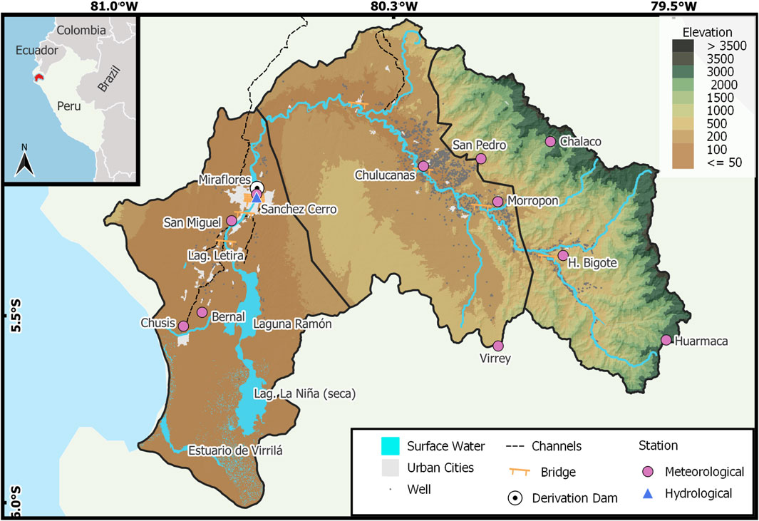
Figure 1. Location of the Piura River basin and hydroclimatological stations. Black lines delineate the upper, middle and lower Piura Basin (from east to west).

Figure 2

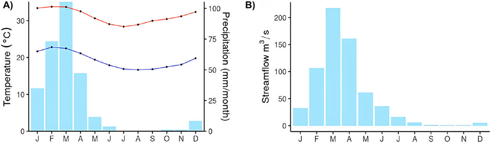
Figure 2. Hydroclimatology of Piura River basin 1981–2020 (A) climograph presenting mean monthly minimum (blue) and maximum (red) temperatures and rainfall (light blue bar) using San Miguel, Miraflores, and Morropon conventional climatological stations record and (B) mean monthly streamflow at Puente Sanchez Cerro hydrological station.

The upper part of the Piura basin is located at higher altitudes and is predominantly characterized by mountain ecosystems, including relict montane forests and páramo. In contrast, the middle and lower parts, which are closer to the coast, feature seasonally dry forests and agricultural areas, representative of the arid and semi-arid ecosystems of northern Peru, also have a diverse range of vegetation types, including dry hill and mountain forests, riparian forests, and even mangrove areas near the coast (MINAM, 2019). (see Supplementary Figure S1). The montane forests are critical in stabilizing soils and reducing runoff, whereas dry forests in the lower-middle basin are highly susceptible to desertification, which is exacerbated by El Niño-related climatic anomalies.

In the upper Piura Basin, agricultural production is diverse, mostly consisting of rice (3,819 ha), corn (2,721 ha), beans (1,168 ha) for local and regional markets, but also mango (3,352 ha), banana (1,399 ha), cacao (811 ha) for export and currently increasing (Autoridad Nacional del Agua (ANA), 2014). It relies on traditional irrigation practices applied by small-holder farmers (Mills-Novoa, 2020). In the upstream part of the middle Piura Basin, the San Lorenzo district benefits from its own reservoir built by the Peruvian government in 1950s with funds from the World Bank in the framework of the Peruvian Agrarian Reform (Lynch, 2019). It allows the production of mangos (16,634 ha) and limes (5,176 ha) destined to export by small-holder farmers (Autoridad Nacional del Agua (ANA), 2014; Lynch, 2019). The middle and lower parts of the Piura Basin are experiencing large agricultural expansion (Mills-Novoa, 2020). Irrigated land increased from 19,140 ha to 28,210 ha (47%) between 2006 and 2013 (Junta de Usuarios: Medio-Bajo Piura, 2011; Junta de Usuarios: Medio-Bajo Piura, 2014), using both surface and poorly regulated groundwater resources, driven by Peruvian and international agro-business investments in large-scale table grape vineyards (Autoridad Nacional de Agua, 2012; Autoridad Nacional del Agua (ANA), 2014; Autoridad Nacional del Agua (ANA), 2015; Autoridad Nacional del Agua (ANA), 2016). In parallel, agricultural productions from small-holder farmers also shifted toward banana, lime, and mango destined to export (Mills-Novoa, 2020). The lower Piura shifted from its historically cotton production to small-scale rice production (8,011 ha) in rotation with corn (5,703 ha) and beans (1,574 ha) for the domestic market (Autoridad Nacional del Agua (ANA), 2014). This area is characterized by extensive drainage and irrigation infrastructures needed for historical cotton production and nowadays intensive land use with two harvests per year (Mills-Novoa, 2020).

The Piura River Basin also experiences strong socioeconomic pressures due to the expansion of agricultural and urban activities, which have led to significant transformations in vegetation cover over recent decades. These pressures, combined with the influence of climatic phenomena such as El Niño, contribute to soil degradation and vegetation loss, especially in vulnerable areas like the seasonally dry forests (Móstiga et al., 2024a; Muenchow et al., 2013). Studies have shown that the expansion of agricultural lands and urbanization are major drivers of deforestation and land cover change in the region, leading to the fragmentation of habitats, decline in biodiversity and increasing vulnerability to flooding (Rau et al., 2022; Rubiños and Anderies, 2020; Torres Ruiz de Castilla, 2010; Móstiga et al., 2024b). Changes in vegetation cover in this region reflect how ecosystems respond to both natural disturbances and human activities, highlighting the need for integrated land management to ensure the conservation of natural resources and the resilience of local ecosystems (Otivo Meza, 2015; Song et al., 2018).

3 Data and methods

3.1 Land cover dataset

For this study, data from the Moderate Resolution Imaging Spectroradiometer (MODIS) and European Space Agency Climate Change Initiative (ESA-CCI) global satellite-based land cover products were used, along with the National Ecosystem Map of Peru (MINAM, 2019). The MODIS product, specifically the Type 1 classification from the International Geosphere-Biosphere Programme (IGBP) (Friedl and Sulla-Menashe, 2022), provides annual global land cover maps at a 500 m resolution from 2001 to the present. In contrast, the ESA-CCI Land Cover dataset (ESA, 2017) offers annual global land cover classifications at a finer 300 m resolution, covering the period from 1992 to 2022. The National Ecosystem Map, developed using Sentinel-2 and Landsat imagery, provides a static, high-resolution reference dataset (30 m resolution) with field-based validation, making it a key resource for evaluating land cover classification accuracy in Peru.

Despite similarities in thematic classification, MODIS and ESA-CCI differ in their methodological approaches and sensitivity to land cover change detection (see Table 1). MODIS applies a Random Forest classification algorithm with smoothed time-series reflectance, which increases sensitivity to interannual changes, including variations in land cover condition (e.g., agricultural cycles or shifts in vegetation density). In contrast, ESA-CCI employs a probability-based classification with a 2-year temporal filter, prioritizing long-term, robust thematic changes and reducing short-term variability. These methodological differences affect the spatial distribution and extent of certain land cover types.

Table 1

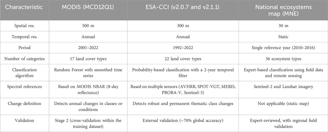
Table 1. Comparison of three LULC datasets: MODIS, ESA-CCI, and the National Ecosystems Map (MNE).

To standardize the classification across datasets Herold et al., 2008, we harmonized the land cover categories into six major classes: Forest, Non-Forest Vegetation, Cropland, Urban, Water Bodies, and Bare Soil (Supplementary Table S1). This aggregation was based on class correspondence between the datasets and further cross-validated using the National Ecosystem Map. Supplementary Table S1 provides a detailed breakdown of how original land cover classes from MODIS and ESA-CCI were assigned to these macroclasses.

Supplementary Figure S1B presents the spatial distribution of these six macroclasses across the three datasets. Notably, MODIS’s Urban and Non-Forest Vegetation classifications show greater similarity to the National Ecosystem Map, while ESA-CCI’s Cropland classification more closely aligns with the mapped agricultural areas in the reference dataset. Additionally, substantial variations exist in the distribution of forested areas among the three datasets, highlighting differences in how each product classifies dense vegetated regions. Bare Soil areas appear more extensive in both ESA-CCI and MODIS compared to the National Ecosystem Map (MINAM, 2019), based on local information satellite images from several sensors acquired over several years, suggesting possible overestimation of barren land in the global datasets.

This standardized classification enables a more robust analysis of land cover changes, facilitating direct comparisons between datasets while maintaining ecological relevance within the Piura River Basin.

3.2 ENSO indices

ENSO indices are defined using Sea Surface Temperature (SST) anomalies in different regions of the Pacific Ocean. In this study, El Niño 1+2, 3 and 4 indices were used. They are computed over regions located in the eastern and central Pacific, between longitudes 80°W and 90°W/90°W and 150°W/150°W and 160°E, and latitudes 0° and 10°S/5°N and 5°S/5°N and 5°S, respectively (Rayner et al., 2003). They are available on a monthly time step starting from January 1870 at: https://psl.noaa.gov/data/timeseries/month/.

3.3 Intensity analysis

Intensity analysis is a method used to understand LULC changes over time by breaking them down into three levels: interval, category, and transition. It compares observed changes to a uniform reference to determine whether certain land transitions are happening more or less frequently than expected. This approach helps differentiate real changes in landscape from variations due to data classification errors and is particularly useful for examining how land cover changes relate to climatic events and human activities (Aldwaik and Pontius, 2012).

The intensity analysis was carried out following the structure proposed by Aldwaik and Pontius (2012) and was implemented using the OpenLand package (Exavier and Zeilhofer, 2020). This paper focuses on the comparison of change rates, the equations for each level of analysis is on Supplementary Material, also for further details, please refer to Aldwaik and Pontius (2012).

To analyze potential influences of climate variability on land cover changes, the study period was divided into two intervals: 2000–2010, characterized by a lower frequency of strong warm events, and 2011–2022, which includes a higher occurrence of El Niño Costero events. This division was selected to balance the length of the time periods while also capturing a shift in climatic patterns, particularly the increased frequency of El Niño events after 2014, as shown in the ENFEN (2024) technical report. Additionally, an annual-scale analysis, included in the Supplementary Material, provides insights into specific years where significant deviations may have occurred.

3.3.1 Interval level analysis

This approach helps to determine whether the rate of change is accelerating or decelerating over time by comparing each interval’s change rate to a uniform reference value. There are two key variables used in this level:

• St (Observed Annual Change Rate): Represents the percentage of land cover change within a specific time interval. If the study period is from 2001 to 2022 using 1-year intervals, there are 21 values of St.

• U (Uniform Annual Change Rate): A single value representing the expected annual change rate if the land cover change were evenly distributed across all intervals. If all St values were the same, they would be equal to U.

By comparing St to U, it is possible to determine whether a particular interval experiences a slower or faster-than-average change rate. If St is below U, the change is relatively slow; if it is above U, the change is relatively fast.

3.3.2 Category level analysis

This analysis examines how land cover changes differ among categories over time. It helps identify whether a specific land cover type is experiencing more gains or losses than expected under a uniform change scenario. The three key variables are used at this level:

• St (Uniform Change Rate for the Interval): Represents the expected change rate if land transitions were evenly distributed.

• Gtj (Gain Intensity): Measures how much a category expands in each time interval.

• Lti (Loss Intensity): Measures how much a category shrinks in each time interval.

If the gain or loss intensity of a category is below (above) the uniform change rate (St), the category is considered inactive (active) during that interval. A category is defined as stationary if its gain or loss intensity rate remains consistently above or below the uniform line across all intervals.

3.3.3 Transition level analysis

The transition level of intensity analysis examines how specific land cover categories transition into or out of each other over time. This level helps determine whether a category tends to systematically gain from or lose to particular categories more than expected under a uniform transition assumption. It’s considered a transition from a “m” category to “n.” Four key variables are used at this level:

• Rtin (Observed Transition Intensity): Measures the actual rate at which category i transitions into category n in a given time interval.

• Wtn (Uniform Transition Gain Intensity): Represents the expected transition rate if category n were to gain uniformly from all other categories in proportion to their initial sizes.

• Qtmj (Observed Transition Loss Intensity): Measures the actual rate at which category m transitions into another category j.

• Vtm (Uniform Transition Loss Intensity): Represents the expected loss rate of category m if its losses were uniformly distributed across all possible receiving categories

If the intensity bar ends to the left (right) of the uniform line, the transition systematically avoids (targets) that category. A transition is classified as stationary if it follows a consistent pattern across all time intervals, meaning it systematically targets, avoids, or remains neutral toward a specific transition over time.

3.4 Correlation with hydroclimatological variables

For the analysis of correlations between land cover and hydroclimatological variables, a Pearson correlation was used considering a 95% confidence interval. The data on land cover was transformed into proportions to normalize the varying extents of land cover categories across the study area. The hydroclimatological variables, from Peruvian Interpolated data of Peruvian hydrometeorological Service (SENAMHI)’s Climatological and hydrological Observations (PISCO-SENAMHI) datasets, included precipitation (Aybar et al., 2020) for the period 2001–2022, and maximum and minimum temperatures (Huerta et al., 2023) for the period 2001–2020. These datasets were averaged over both the upper and mid-lower catchments of the Piura basin.

To take into account large-scale climatic patterns, the two atmospheric El Niño indices E (Eastern Pacific) and C (Central Pacific), defined by (Takahashi et al., 2011) were included in the correlation analysis. The E index is calculated as approximately 1.7×Niño₄ − 0.1×Niño₁₊₂, capturing El Niño events centered in the Eastern Pacific, while the C index (Niño₄ + 0.5×Niño₃ − 0.5×Niño₁₊₂) reflects events centered in the Central Pacific (Takahashi et al., 2011). Additionally, the Coastal El Niño Index (ICEN), based on Niño1+2, with 1990–2020 climatology was incorporated to capture regional coastal variability (ENFEN, 2024) and served to assess the impacts of coastal El Niño and La Niña events on vegetation cover. These three indices were calculated using the DJF (Dec-Jan-Feb) seasonal averages (Supplementary Table S2). The correlations were conducted separately for the wet (December–May) and dry (June–September) season to account for seasonal variability in both land cover and hydroclimatological dynamics, also they were correlated for different time lags and leads, particularly focusing on a 1-year lead or lag for the climatic indices to assess delayed or anticipatory impacts on land cover.

4 Results

4.1 Spatial and temporal analysis of LULC

Land use and land cover (LULC) changes analysis in the Piura Basin from 2001 to 2022 was conducted using MODIS and CCI products, allowing the evaluation of spatial distribution and temporal evolution. The results show that Non-Forest Vegetation is the dominant category throughout the study period, with significant differences in the detection of changes between the two products.

In the upper basin, MODIS (Figure 3A) shows a clear predominance of Non-Forest Vegetation, with noticeable variability over time, particularly when compared to Forest, which also experiences large fluctuations. In contrast, Cropland and Urban areas remain more stable across the years. The lower-middle basin (Figure 3B) presents a similar pattern, where Non-Forest Vegetation is the most widespread category, followed by Bare Soil and Cropland, which exhibit higher interannual variability. The CCI product, on the other hand, presents a lower (higher) area of Non-Forest Vegetation (Forest) in the upper basin, respectively (Figure 3C), with a smoother temporal evolution. In the lower-middle basin (Figure 3D), Bare Soil dominates slightly over Non-Forest Vegetation, with changes remaining relatively small except for a visible shift between 2001 and 2002–2003.

Figure 3

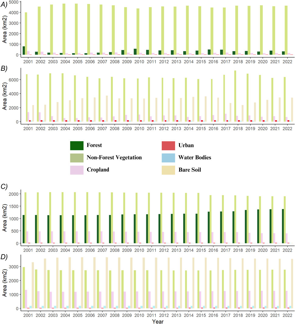
Figure 3. Temporal changes in LULC categories from 2001 to 2022 for MODIS (A,B) and CCI (C,D) LULC products. Panels (A) and (C) correspond to the upper basin, while panels (B) and (D) correspond to the lower-middle basin.

When evaluating the magnitude of land cover changes (Figure 4), the MODIS product shows that 67.2% of the basin remained unchanged, while CCI indicates a significantly higher stability, with 93.2% of the area without change s. The percentage of the area experiencing up to five changes between 2011 and 2022 is 29.2% in MODIS and 6.8% in CCI, suggesting that MODIS captures more frequent LULC variations. Notably, only MODIS identifies a 3.6% area undergoing more than five changes, primarily concentrated in the upper basin, near the curved section of the watershed. The areas experiencing three to five changes are mostly located in the lower basin, whereas the most stable regions are found in the central part of the basin.

Figure 4

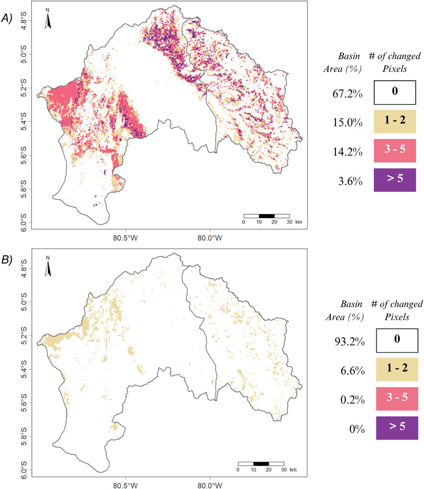
Figure 4. Number of changed pixels from 2001 to 2022 and the percentage of the basin with that number of changes, using MODIS (A) and CCI (B) LULC products.

For the CCI product, changes are mostly limited to one to two transitions, mostly occurring in the upper and lower basins, while the central region remains the most stable. These discrepancies highlight the differences in sensitivity between the two products, with MODIS detecting more dynamic and frequent changes, while CCI provides a more stable representation of LULC evolution over the 22-year period. This variation suggests that MODIS is more responsive to short-term changes, potentially related to seasonal fluctuations or land management practices, whereas CCI offers a broader perspective on long-term transitions.

4.2 LULC intensity analysis by interval level

This section presents the analysis of land use changes in the upper and lower-middle catchments of Piura basin using the MODIS and CCI product, focusing on the temporal intensity of these changes.

4.2.1 Upper Piura Basin

The analysis of land cover change in the upper Piura basin reveals notable differences between MODIS and CCI, particularly in the magnitude of detected changes (Figure 5). The uniform annual change intensity (U) for MODIS is 4.9%, which is ten times higher than the 0.4% reported by CCI. This means that the total area affected by land cover change per year is ten times larger in MODIS than in CCI, indicating that MODIS detects more extensive transformations across the landscape.

Figure 5

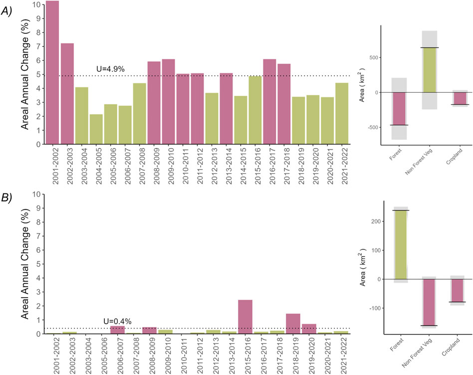
Figure 5. Annual land cover change rates for the upper basin using MODIS (A) and CCI (B) LULC data from 2001 to 2022. Bars represent the percentage of area change per year, with rapid changes highlighted in pink and slower changes in green. The dashed line indicates the uniform annual change intensity (U).

Despite differences in change magnitude, both datasets consistently identify 2008–2009 as a period of rapid land cover change, reinforcing the reliability of this transition. Additionally, both MODIS and CCI indicate a net loss of cropland over the study period, suggesting a sustained decline in agricultural land use in the upper basin. However, discrepancies arise in the net balance of Forest and Non-Forest Vegetation. MODIS shows a net rapid loss of Forest cover and a net slower gain of Non-Forest Vegetation, whereas CCI presents the opposite behavior, with a slow net gain in Forest cover and a rapid net loss in Non-Forest Vegetation.

4.2.2 Lower-middle Piura Basin

In the lower-middle basin, the magnitude of land cover change differs considerably between MODIS and CCI, with MODIS reporting a uniform annual change intensity (U) of 4.7%, compared to only 0.3% in CCI (Figure 6). This indicates that the total area affected by land cover change per year is 15 times larger in MODIS than in CCI, suggesting that MODIS detects a significantly more intense transformation of land cover over time. While MODIS captures more detailed interannual variations, CCI portrays a more stable landscape, meaning that MODIS is more sensitive to detecting smaller or transient changes, while CCI provides a more conservative estimate of long-term land cover transitions.

Figure 6

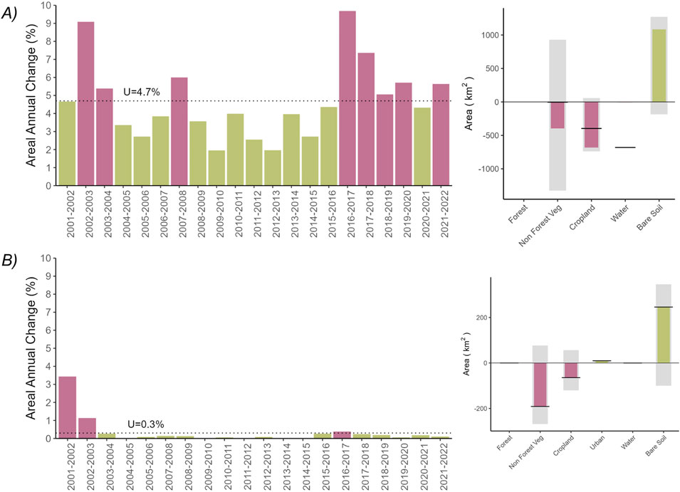
Figure 6. Annual land cover change rates for the lower-middle basin using MODIS (A) and CCI (B) LULC data from 2001 to 2022. Bars represent the percentage of area change per year, with rapid changes highlighted in pink and slower changes in green. The dashed line indicates the uniform annual change intensity (U).

Despite these differences, both datasets identify 2002–2003 and 2016–2017 as key periods of rapid land cover change, suggesting that significant transformations occurred in these years. Additionally, while MODIS and CCI differ in the magnitude of detected changes, they consistently indicate the same overall land cover trends. Both datasets show a rapid net loss of Non-Forest Vegetation and Cropland, along with a slower net gain in Bare Soil.

4.3 LULC intensity analysis by categories level

The analysis of land use and land cover (LULC) intensity at the category level provides a detailed assessment of the relative gains and losses of different land cover types in the Piura basin. By comparing decadal time periods (2001–2011 and 2011–2022, Figure 6) with annual variations (Supplementary Material), it is possible to determine which categories exhibit systematic changes and whether their behavior remains stationary over time.

4.3.1 MODIS LULC product

Intensity analysis using MODIS data identified clear differences in land cover change between the upper and mid-lower Piura basins across two broad intervals (2001–2011 and 2011–2022) (Figure 7A). In the upper basin, the first interval (2001–2011) exhibited roughly twice the change intensity (St = 1.87%) compared to the second interval (2011–2022, St = 0.89%), despite a similar duration. Non-Forest vegetation gained the largest absolute area during 2001–2011 but consistently remained below the uniform intensity threshold (St). Conversely, Forest and Cropland frequently exceeded St, highlighting significant relative dynamics. Specifically, Forest exhibited non-stationary behavior, shifting from below St in 2001–2002 to consistently surpassing it from 2002 to 2003 onward. Cropland showed pronounced gains surpassing St in periods such as 2007–2009 and 2014–2017 (Supplementary Figure S2). Water bodies exhibited notable losses surpassing St during 2009–2010, 2012–2013, and 2016–2017, while Forest recorded significant losses particularly in 2001–2002, 2010–2011, 2012–2013, and 2016–2018, although without substantial absolute area reductions.

Figure 7

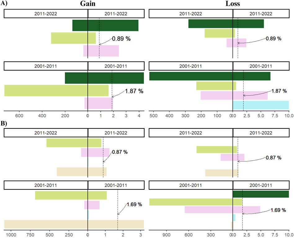
Figure 7. Spatial gains and losses by land cover category in the upper (A) and mid-lower (B) Piura basin for the intervals 2001–2011 and 2011–2022, using MODIS LULC data. The left-side graphs show gains, while the right-side graphs represent losses. The dashed line indicates the uniform change intensity (St). Forest appears in dark green, Non-Forest vegetation in light green, Cropland in pink, Urban in red, water bodies in light blue, bare soil in beige.

Annual-scale analysis (Supplementary Figure S2) highlighted that the most intense year for land cover changes in the upper basin was 2001–2002 (St = 14.29%), followed by marked peaks during 2008–2010 and 2016–2018. Gains in Forest and Non-Forest categories revealed a pattern of stationarity, consistently remaining either above or below the uniform threshold, with Forest showing fluctuations around clear peak years (e.g., 2008–2009). Cropland displayed notable annual losses predominantly in 2002–2003 and 2017–2018, while Non-Forest losses peaked notably in 2008–2009 and 2015–2016.

In the mid-lower basin, the first period (2001–2011, St = 1.69%) also presented nearly double the change intensity compared to the second period (2011–2022, St = 0.87%) (Figure 7B). Cropland exhibited a non-stationary pattern, transitioning from below St in the first interval to above it in the second, indicating an intensification of agricultural expansion after 2011. Urban expansion also increased notably during the second interval. Forest losses exceeded St only in the first interval and were negligible thereafter. Bare Soil showed minimal change in the upper basin but displayed pronounced dynamics in the mid-lower basin, consistently surpassing St from 2015 onward, indicating ongoing transformation towards other land cover types.

Annual variations (Supplementary Figure S3) in the mid-lower basin revealed intense gains in Non-Forest vegetation notably in 2002–2003, 2007–2008, and 2016–2018, while Bare Soil gains peaked during 2002–2003, 2006–2007, and 2018–2019. Cropland gains occurred prominently in 2005–2006, 2008–2009, and 2016–2017. Losses in Non-Forest vegetation were significant primarily during 2002–2003 and from 2018 to 2021, whereas Cropland losses were prominent across multiple years (2002–2003, 2010–2011, 2013–2014, 2017–2018, and 2019–2020). Bare Soil recorded notable losses mainly during 2007–2008 and 2016–2017.

4.3.2 CCI LULC product

Intensity analysis using CCI LULC data revealed clear differences in land cover dynamics between the upper and mid-lower Piura basins across two broad intervals: 2001–2011 and 2011–2022 (Figure 8). In the upper basin, the period 2011–2022 showed significantly greater change intensity (St = 0.53%) compared to the earlier interval, 2001–2011 (St = 0.17%), with this difference evident for both land gains and losses. Forest and cropland displayed stationary behaviors regarding gains, with only forest consistently surpassing the uniform intensity threshold (St) during the second interval, while cropland remained consistently below it. In contrast, urban areas did not exhibit stationarity, appearing with notable intensity only during 2011–2022. Non-forest vegetation experienced significant losses in 2011–2022, clearly exceeding St, and bare soil losses also appeared during this time period, although without surpassing St, indicating transformations from exposed land to other land cover types.

Figure 8

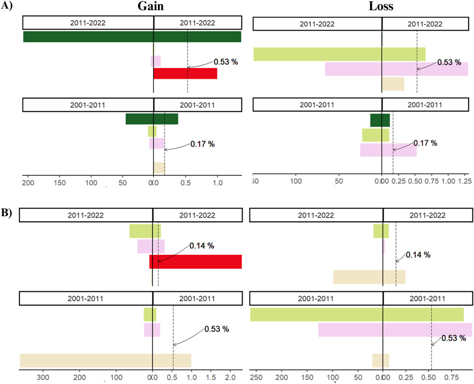
Figure 8. Spatial gains and losses by land cover category in the upper (A) and mid-lower (B) Piura basin for the intervals 2001–2011 and 2011–2022, using CCI LULC data. The left-side graphs show gains, while the right-side graphs represent losses. The dashed line indicates the uniform change intensity (St). Forest appears in dark green, Non-Forest vegetation in light green, Cropland in pink, Urban in red, water bodies in light blue, bare soil in beige.

The annual-scale analysis (Supplementary Figure S6) in the upper basin highlighted that the most intense land cover changes occurred between 2015 and 2021. Urban areas showed the highest intensity gains in 2016–2017 and 2020–2021, despite their relatively limited spatial extent. Forest gained consistently above St from 2011 onwards, reaching a peak in 2015–2016. Non-forest vegetation recorded its highest losses in 2015–2016 and 2018–2019, while cropland’s greatest losses were observed in 2018–2019. Bare soil surpassed St only in gains for 2001–2002 and in losses for 2020–2021, though with minimal area impact. Water exhibited minimal losses, with noticeable intensity only in specific years, such as 2002–2003.

In the mid-lower basin, the first period (2001–2011, St = 0.53%) had a significantly higher intensity of land cover changes, approximately four times greater than in the subsequent interval (2011–2022, St = 0.14%). No land cover category displayed stationary behavior throughout the entire study period. There was a clear net gain of bare soil during the first interval, aligned with notable losses in non-forest vegetation and cropland, clearly illustrated in Figure 6. Urban area gains progressively increased after 2011, while the highest gains for non-forest vegetation occurred during 2016–2017. Annual variations (Supplementary Figure S7) showed peak gains for bare soil in 2001–2002 and 2002–2003, coinciding with the highest losses in non-forest vegetation and cropland during the same years. These patterns underscore substantial land cover transitions, particularly in the early 2000s, highlighting distinct dynamics compared to the upper basin. Loss intensity for non-forest vegetation was particularly pronounced in the early years, while cropland losses were distributed across various years, emphasizing ongoing agricultural land-use shifts.

4.4 LULC intensity analysis by transition level

The transition analysis at the category level reveals essential dynamics of land use and land cover changes across both the lower-middle and upper basins. This section will describe these transitions, focusing on gains and losses across the same group periods from the previous analysis.

4.4.1 MODIS LULC product

In the upper basin, MODIS data showed distinct transition patterns (Figure 9A). Non-Forest vegetation predominantly gained area from Forest, surpassing the uniform transition intensity (Wtn = 6.46% for 2001–2011 and Wtn = 4.64% for 2011–2022) in both intervals. Cropland exceeded the uniform transition intensity only during 2001–2011, while Water exceeded the threshold solely in this interval. Regarding Cropland losses, transitions predominantly targeted Non-Forest vegetation, significantly surpassing the uniform transition intensity (Vtm = 0.41%) during the first interval and showing a marked reduction in the second interval (Vtm = 0.07%).

Figure 9

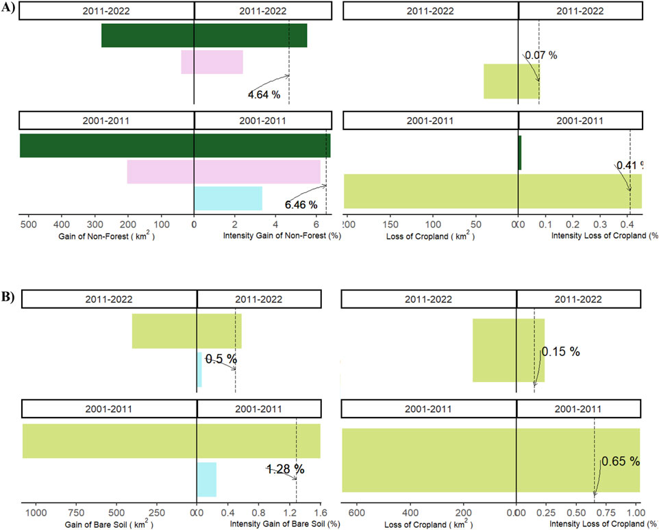
Figure 9. Transition intensity analysis for the loss of cropland and gain of bare soil in the Upper (A) and Lower-Middle (B) Piura basin over two intervals from 2001 to 2022 (MODIS). The dashed line represents the uniform loss transition intensity (Vtm), which indicates the expected intensity of losses from each land cover category if changes were uniformly distributed across all possible transitions. Forest appears in dark green, Non-Forest vegetation in light green, Cropland in pink, Urban in red, water bodies in light blue, bare soil in beige.

Annual-scale analysis for the upper basin (Supplementary Figure S4) showed intense gains for Non-Forest vegetation, particularly in 2001–2002 (Wtn = 56.66%) and 2017–2018 (Wtn = 35.09%), with contributions mainly from Forest and Cropland categories. Forest frequently surpassed the uniform intensity threshold, except during 2008–2010 and 2012–2013, when it either stayed at or slightly below this threshold. Cropland transitions to Non-Forest vegetation surpassed the threshold notably during 2008–2010 and aligned with the threshold during 2003–2004 and 2012–2013, remaining below in other years. In terms of Cropland losses, transitions exclusively targeted Non-Forest vegetation, consistently surpassing or matching the uniform intensity threshold. The highest intensity was observed in 2002–2003 (Vtm≈2.4%), while in several years (2004–2006, 2017–2018, 2018–2019, and 2020–2021), transition intensity aligned closely with the uniform rate.

In the mid-lower basin, MODIS data also exhibited clear transition dynamics (Figure 9B). Bare Soil gains were primarily driven by transitions from Non-Forest vegetation, which significantly exceeded the uniform transition intensity (Wtn = 1.28%) in the first interval (2001–2011). During the second interval (2011–2022; Wtn = 0.5%), transitions into Bare Soil were minimal. Cropland losses consistently favored Non-Forest vegetation, surpassing the uniform intensity threshold in both intervals (Vtm = 0.65% for 2001–2011 and Vtm = 0.15% for 2011–2022), although transitions were notably more intense during the first interval.

Annual-scale analysis for the mid-lower basin (Supplementary Figure S5) revealed significant variations in Bare Soil gain intensity. Years with the highest uniform transition intensities included 2019–2020 (Wtn = 4.83%), 2018–2019 (Wtn = 4.67%), and 2002–2003 (Wtn = 4.54%). Non-Forest vegetation frequently surpassed the uniform intensity threshold in most years, except during 2016–2017, 2011–2012, and 2007–2008, when it matched the threshold, and 2009–2010, when it was slightly below. Water transitions into Bare Soil exceeded the uniform threshold during multiple intervals (2002–2003, 2007–2008, 2009–2013, and 2015–2018), whereas it remained below or absent in other years. For Cropland losses, transitions exclusively targeted Non-Forest vegetation, consistently exceeding the uniform transition intensity threshold (Vtm). The highest intensities were recorded in 2002–2003 (Vtm = 5.65%), followed by notable peaks in 2010–2011 (Vtm = 2.97%), 2013–2014 (Vtm = 2.25%), and 2017–2018 (Vtm = 3.25%).

4.4.2 CCI LULC product

Transition-level intensity analysis with the CCI dataset highlighted different land cover dynamics between the upper and mid-lower basins for two intervals: 2001–2011 and 2011–2022 (Figure 10).

Figure 10

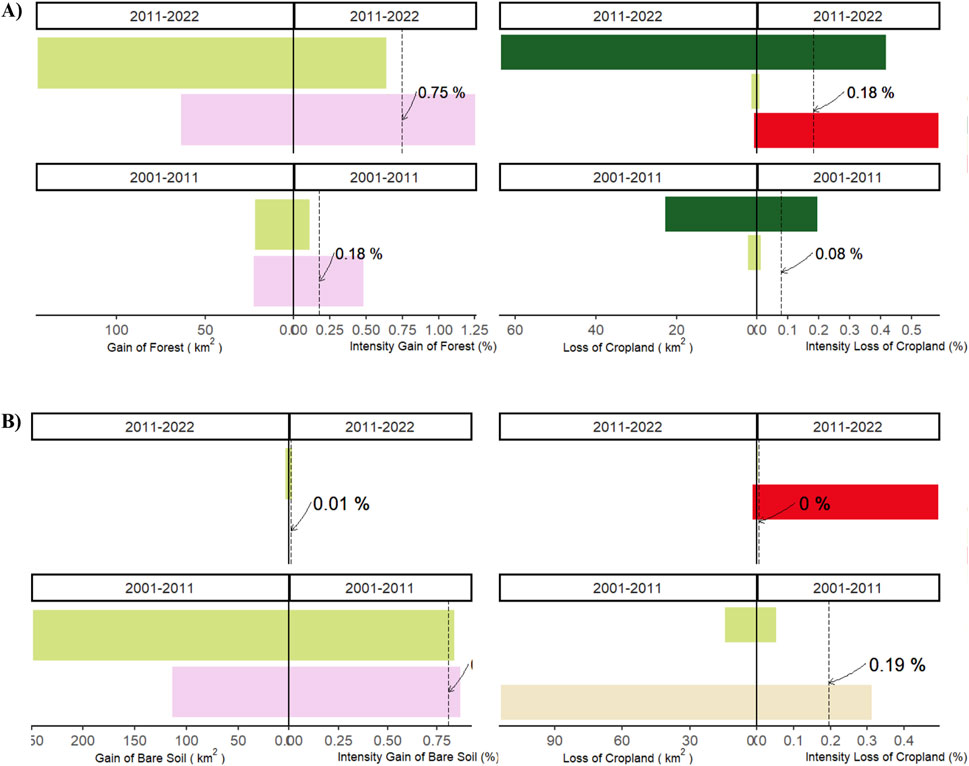
Figure 10. Transition intensity analysis for the loss of cropland and gain of bare soil in the Upper (A) and Lower-Middle (B) Piura basin over two intervals from 2001 to 2022 (CCI). The dashed line represents the uniform loss transition intensity (Vtm), which indicates the expected intensity of losses from each land cover category if changes were uniformly distributed across all possible transitions. Forest appears in dark green, Non-Forest vegetation in light green, Cropland in pink, Urban in red, water bodies in light blue, bare soil in beige.

In the upper basin, forest gains predominantly originated from non-forest vegetation and cropland. During 2001–2011 (Wtn = 0.18%), cropland significantly exceeded the uniform intensity, while in 2011–2022 (Wtn = 0.75%), non-forest vegetation was the primary contributor surpassing the uniform rate. Annual analysis (Supplementary Figure S8) indicated peak forest gains in 2015–2016 (3.5%) mainly from non-forest vegetation, and in 2018–2019 (2.2%) primarily from cropland. Cropland consistently contributed modestly from 2006 to 2010. Regarding cropland losses, forest consistently exceeded the uniform intensity rate in both intervals (Vtm = 0.08% for 2001–2011 and Vtm = 0.18% for 2011–2022), with urban areas surpassing the threshold only during 2016–2017 and 2020–2022. The highest annual intensities of cropland loss occurred in 2018–2019 (0.89%) and 2019–2020 (0.45%).

In the mid-lower basin, bare soil gained mainly from cropland and non-forest vegetation during the earlier interval (2001–2011, Wtn = 0.8%), with cropland consistently exceeding the uniform intensity rate. However, during the later interval (2011–2022, Wtn = 0.01%), intensity gains were minimal, with no significant category surpassing the uniform intensity. Annual analysis (Supplementary Figure S9) showed a marked decreasing trend in bare soil gains from 2001 to 2002 (5%) to 2003–2004 (0.49%). Cropland was the dominant contributor in the earliest years (2001–2003), after which it disappeared from contributing categories. Non-forest vegetation exceeded slightly the uniform rate in 2001–2002 and 2003–2004. Regarding cropland losses, bare soil consistently surpassed the uniform rate (Vtm = 0.19%) in 2001–2002 (1.34%) and 2002–2003 (0.6%), accompanied by minimal contributions from non-forest vegetation. Loss intensities remained negligible post-2004, with urban areas appearing marginally after 2012.

4.5 Correlation with climate variables and LULC categories

The relationship between land cover changes and hydroclimatic variables was analyzed separately for the lower-middle and upper Piura basin, considering both MODIS and CCI products. The results presented in Tables 2, 3 show only statistically significant correlations that passed the 95% confidence threshold.

Table 2

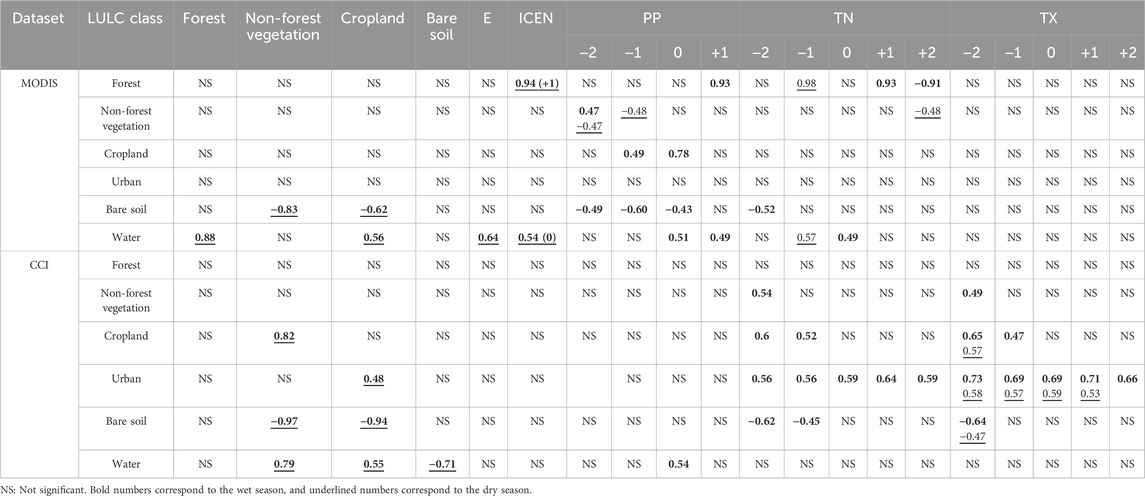
Table 2. Significant (95%) correlation values between land cover categories and hydroclimatic variables in the lower-middle basin. E index, PP (precipitation), TN (minimum temperature), and TX (maximum temperature) with indicated yearly lags.

Table 3

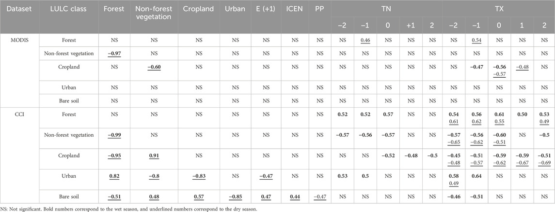
Table 3. Significant (95%) correlation values between land cover categories and hydroclimatic variables in the upper basin. E index, PP (precipitation), TN (minimum temperature), and TX (maximum temperature) with indicated yearly lags.

4.5.1 Lower-middle basin analysis

In the lower-middle basin, both MODIS and CCI consistently indicated strong relationships between certain land cover types, particularly Bare Soil, Non-Forest Vegetation, and Cropland. A strong negative correlation was found between Bare Soil and Non-Forest Vegetation (−0.83 MODIS; −0.97 CCI) and between Cropland and Bare Soil (−0.62 MODIS; −0.94 CCI). Cropland and Water had a positive correlation (0.56 MODIS; 0.55 CCI).

Differences emerged between MODIS and CCI concerning their detection of hydroclimatic influences. MODIS showed stronger correlations with ENSO indices (E and ICEN) and precipitation (PP), while CCI had more significant correlations with maximum (TX) and minimum (TN) temperatures. Notably, the Forest category correlated positively with ICEN at a 1-year lead (0.94 MODIS), and Water correlated positively with E (0.64) and ICEN (0.54) without lag. Cropland showed a strong positive correlation with precipitation (0.78, no lag), whereas Bare Soil had a negative correlation (−0.6, 1-year lag).

Regarding temperature, MODIS showed strong correlations between Forest and minimum temperature (TN), specifically at 1-year lead (0.93), 2-year lead (−0.91), and 1-year lag (0.98). CCI presented lower-magnitude correlations with minimum temperature around 0.6 for Urban (lead 1), Cropland (lag 1 or 2), and Bare Soil (−0.6, 2-year lag). Urban areas showed a strong correlation with maximum temperature (TX), particularly in MODIS (0.7).

4.5.2 Upper basin analysis

In the upper basin, correlations between land cover categories and climate variables showed different patterns compared to the lower-middle basin. Strong negative correlations existed between Forest and Non-Forest Vegetation (−0.97 MODIS; −0.99 CCI) and between Cropland and Forest (−0.95 CCI). Urban expansion correlated positively with Forest (0.82), and negatively with Non-Forest Vegetation (−0.8), Cropland (−0.83), and Bare Soil (−0.85). Cropland and Non-Forest Vegetation correlated positively (0.91).

MODIS had fewer significant correlations with climate variables in the upper basin compared to CCI. However, Cropland negatively correlated with maximum temperature (TX) between −0.47 and −0.57 (lag 0 and +1), and Forest positively correlated with TX at 1-year lag (0.54).

CCI identified numerous significant correlations: Forest and minimum temperature (TN) had a positive correlation (0.57), while Non-Forest Vegetation and Cropland negatively correlated with TN (−0.57 and −0.52, respectively). Urban areas correlated positively with TN (0.50, lag 1). For maximum temperature (TX), Forest had a positive correlation (0.61), whereas Non-Forest Vegetation, Cropland, and Bare Soil showed negative correlations (−0.6, −0.6, and −0.51, respectively). Urban areas correlated positively with TX (0.64, lag 1). Precipitation negatively correlated with Bare Soil during the dry season (−0.47, CCI). Urban areas negatively correlated with the E index (−0.47, lag 1), and Bare Soil positively correlated with E (0.47, lag 1) and ICEN (0.44). Most significant correlations in the upper basin occurred during the wet season.

5 Discussion

The results highlight substantial differences between the MODIS and ESA-CCI datasets, primarily due to their classification methodologies, temporal resolutions, and detection sensitivities. MODIS exhibits greater sensitivity to interannual spectral variations, capturing more frequent land cover transitions, ranging from actual thematic class changes to more likely conditional changes in land cover that fall short of full conversion. In contrast, ESA-CCI provides a more stable representation of longer-term land cover transformations. These discrepancies align with previous studies emphasizing the impact of classification algorithms and temporal resolution in land cover mapping (Song et al., 2018; Friedl and Sulla-Menashe, 2022). While MODIS detects a higher number of land cover changes, these transitions may include both thematic class shifts and spectral condition variations (Wulder et al., 2018). ESA-CCI, by applying a 2-year temporal filter, prioritizes persistent land cover changes, reducing short-term fluctuations. This distinction is particularly relevant when interpreting land cover change percentages, as MODIS may overestimate short-term changes that do not necessarily reflect persistent transitions (Hansen et al., 2013).

The results also reveal clear differences in the stability of land cover changes detected by MODIS and ESA-CCI. MODIS captures more dynamic transitions, whereas ESA-CCI presents a more stable representation of land cover trends. This is evident in the magnitude of changes observed, where 67.2% of the basin remained unchanged in MODIS, compared to 93.2% stability in ESA-CCI. Additionally, MODIS identified more frequent transitions, with 29.2% of the basin undergoing up to five changes, versus only 6.8% in ESA-CCI. Notably, only MODIS detected areas with more than five transitions (3.6% of the basin), concentrated in the upper watershed near regions with complex topography. These differences highlight the impact of classification methodology on change detection, where MODIS, with its annual classification, is more sensitive to transient changes, capturing short-term fluctuations that likely exceed typical seasonal variability, such as atypical agricultural shifts or unexpected vegetation loss events. In contrast, ESA-CCI applies a temporal smoothing approach, filtering out short-term changes and emphasizing longer-term trends.

The quality of the classification approaches can also be affected by the cloud cover conditions over the study area. Northern Peru is characterized by the presence of mesoscale convective systems responsible for a dense cloud cover (Horel and Cornejo-Garrido, 1986; Goldberg et al., 1987; Jaramillo et al., 2017), especially during the rainy season from January to April (Figure 2A). As both MODIS and ESA CCI LULC are derived from multispectral images, the estimate of land cover classes is strongly affected by the unavailability of valid data during a large part of the year, increasing the risk of misclassification.

Importantly, the intensity analysis (Aldwaik and Pontius, 2012) helps discern between systematic and potentially permanent changes versus transient fluctuations or thematic classification errors. This analytical approach effectively distinguishes real thematic transitions from temporary variations in land cover conditions, particularly relevant in semi-arid regions like the Piura River Basin, where climatic variability and seasonal cycles can strongly influence vegetation dynamics.

The spatial heterogeneity of the Piura River Basin also plays a key role in land cover dynamics. The upper basin, characterized by steeper slopes, lower temperatures, and more stable vegetation cover, exhibits fewer detected changes, particularly in forested and non-forested vegetation categories. In contrast, the lower basin, where cropland expansion and urban growth are more prominent, shows greater variability, especially in cropland and bare soil classes. These patterns align with the distinct precipitation regimes across the basin, where the upper basin receives orographic rainfall, whereas the lower basin is more sensitive to ENSO-driven precipitation variability (Bourrel et al., 2015).

The relationship between ENSO events and land cover change is particularly relevant given the increased frequency of warm events after 2014 (ENFEN, 2024). The division of the study period into 2001–2011 and 2011–2022 effectively captures this shift, with the second period including intense El Niño events, such as the 2015–2016 strong El Niño and the 2017 moderate El Niño. During the 2015–2016 event, there was a notable expansion of bare soil, particularly in the lower basin, where prolonged dry conditions and extreme hydroclimatic stress likely led to vegetation loss and soil degradation (Cai et al., 2020; Rodríguez-Morata et al., 2018). Similarly, post-2017 recovery phases correspond to increases in non-forest vegetation, indicating temporary regrowth responses after extreme precipitation events. Conversely, strong La Niña events, such as those in 2007, 2013, and 2021–2022, appear to have contributed to reductions in cropland extent and an increase in bare soil, reflecting drier conditions and potential land abandonment (Cai et al., 2020; Salazar Zarzosa, 2018). These findings align with previous studies highlighting ENSO’s role in shaping land cover dynamics in northern Peru (Takahashi and Martínez, 2019).

The comparison between MODIS, ESA-CCI, and the National Ecosystem Map of Peru reveals systematic differences in the LULC classes. MODIS’s urban and non-forest vegetation classifications align more closely with the National Ecosystem Map, while ESA-CCI’s cropland classification better matches agricultural zones. Yet, only CCI exhibits a slight increase in urban areas in both the upper (0.53%) and mid-lower (0.14%) Piura Basin (Figure 8) which can reflect the demographic growth in urban areas, with an increase of the people in Piura city of 2.3% between 2013 and 2017 (Zuchetti and Freundt, 2018). The increase in urban areas might have been missed in MODIS LULC due to its coarser spatial resolution as Piura city, the largest city in the Piura Basin has 70% of its urbanized land occupied by informal or spontaneous constructions (Rivera Saavedra, 2016), which might be fragmented. However, the most notable discrepancy is in the extent of bare soil, significantly larger in MODIS and ESA-CCI compared to the National Ecosystem Map. This difference likely results from spatial resolution variations, as the 30-m resolution of the National Ecosystem Map enables finer-scale classification, whereas the coarser 300-m and 500-m resolutions of ESA-CCI and MODIS, respectively, may lead to an overgeneralization of barren areas (Hansen et al., 2013). Additionally, classification methodologies differ, with MODIS using smoothed time-series reflectance and ESA-CCI applying a probability-based classification with a 2-year temporal filter, both of which can overestimate persistent barren landscapes (Giri et al., 2013). Thematic classification discrepancies also contribute to these differences, as the coastal desert category in the National Ecosystem Map includes sparse vegetation patches, which MODIS and ESA-CCI classify as bare soil, leading to apparent barren area overestimation. These findings emphasize the importance of integrating high-resolution regional datasets for land cover validation, reinforcing previous studies highlighting the limitations of coarse-resolution global land cover products in heterogeneous landscapes (Song et al., 2018). Nevertheless, they provide consistent annual changes for cropland (rapid decrease) in the upper Piura Basin (Figure 5) and for forest (slow increase), non forest vegetation and cropland (rapid decrease) in the middle-lower Piura Basin (Figure 6).

Future research should consider combining these products with higher-resolution sensors such as Sentinel-1 and 2 to improve cropland expansion and deforestation detection. Additionally, expanding in-situ validation efforts would most likely enhance classification accuracy, particularly in highly heterogeneous landscapes like the Piura River Basin. Integrating multiple datasets would enable a more comprehensive understanding of land cover change, capturing short-term fluctuations and long-term transformations. Further research should also explore the incorporation of climate indices, such as the Coastal El Niño Index (ICEN), into land cover change models to quantify ENSO’s direct influence on vegetation dynamics.

6 Conclusion

This study analyzed land cover changes in the Piura River Basin from 2001 to 2022 using MODIS, ESA-CCI, and the National Ecosystem Map of Peru, harmonizing their classifications into six macroclasses to enable a standardized comparison. The results highlight significant differences between the global satellite-based products, which are primarily attributed to their classification methodologies, temporal resolution, and detection sensitivity.

MODIS exhibits greater sensitivity to interannual changes, capturing more frequent land cover transitions, which may also include conditional changes within a specific land cover class. ESA-CCI presents a more stable representation of longer-term land cover changes due to its probability-based classification and 2-year temporal filter. These differences led to notable discrepancies in certain categories, particularly in the extent of Bare Soil, which is more extensive in MODIS and ESA-CCI compared to the National Ecosystem Map. The observed inconsistencies underscore the importance of integrating high-resolution regional datasets to refine global land cover assessments.

The division of the study period into 2001–2011 and 2011–2022 reveals an increase in land cover dynamics during the second period, which coincides with a higher frequency of El Niño events after 2014. These climatic fluctuations influenced the expansion of Bare Soil and the reduction of Cropland during strong warm phases, particularly in the lower basin, highlighting the sensitivity of land use dynamics to ENSO-driven hydroclimatic variability. The distinct precipitation regimes and elevatio nal gradients across the upper and lower basins further contribute to spatial heterogeneity in land cover transitions.

The findings of this study emphasize the need for multi-source data integration in land cover change analysis. While MODIS is valuable for detecting short-term variability, ESA-CCI provides a long-term, stable baseline for monitoring gradual transformations. Future research should combine these products with higher-resolution sensors such as Sentinel-3, enabling more precise assessments of cropland expansion, deforestation, and ecosystem degradation. Additionally, integrating climate indices like the Coastal El Niño Index (ICEN) could improve understanding of ENSO-driven land cover changes. Strengthening in-situ validation efforts would also enhance classification accuracy, ensuring more reliable assessments for land management and conservation planning in climate-sensitive regions like the Piura River Basin.

Data availability statement

Publicly available datasets were analyzed in this study. This data can be found here: https://developers.google.com/earth-engine/datasets/catalog/MODIS_061_MCD12Q1?hl=es-419.

Author contributions

FC: Data curation, Formal Analysis, Investigation, Methodology, Software, Validation, Visualization, Writing – original draft, Writing – review and editing. PR: Conceptualization, Funding acquisition, Project administration, Supervision, Writing – review and editing. LB: Writing – review and editing, Supervision. FF: Writing – review and editing.

Funding

The author(s) declare that financial support was received for the research and/or publication of this article. This work was supported through the ePIURA project N°084-2018-FONDECYT-BM-IADT-MU PROCIENCIA.

Acknowledgments

We thank the ePIURA project team for their valuable comments and helpful advice during the process of this research. PR acknowledges the support from KF400238 British Academy: “Furia de los Rios” project. We thank two reviewers for their constructive comments which helped us improve the quality of our manuscript.

Conflict of interest

The authors declare that the research was conducted in the absence of any commercial or financial relationships that could be construed as a potential conflict of interest.

The author(s) declared that they were an editorial board member of Frontiers, at the time of submission. This had no impact on the peer review process and the final decision.

Generative AI statement

The author(s) declare that Generative AI was used in the creation of this manuscript. The corresponding author verifies and takes full responsibility for the use of generative AI in the preparation of this manuscript. Generative AI was used specifically for the purposes of image quality enhancement and translation assistance.

Publisher’s note

All claims expressed in this article are solely those of the authors and do not necessarily represent those of their affiliated organizations, or those of the publisher, the editors and the reviewers. Any product that may be evaluated in this article, or claim that may be made by its manufacturer, is not guaranteed or endorsed by the publisher.

Supplementary material

The Supplementary Material for this article can be found online at: https://www.frontiersin.org/articles/10.3389/frsen.2025.1529044/full#supplementary-material

References

Aber, J., Neilson, R. P., McNulty, S., Lenihan, J. M., Bachelet, D., and Drapek, R. J. (2001). Forest processes and global environmental change: predicting the effects of individual and multiple stressors. Biosci. 51 (9), 735–751. doi:10.1641/0006-3568(2001)051[0735:fpagec]2.0.co;2

CrossRef Full Text | Google Scholar

Aldwaik, S. Z., and Pontius, R. G. (2012). Intensity analysis to unify measurements of size and stationarity of land changes by interval, category, and transition. Landsc. Urban Plan. 106, 103–114. doi:10.1016/j.landurbplan.2012.02.010

CrossRef Full Text | Google Scholar

Atarama, E., and Rashid, M. M. (2019). “Integral management for Piura River basin in Peru,” in Proceedings of the 38th IAHR World Congress. 38 1621–1631. doi:10.3850/38WC092019-1006

PubMed Abstract | CrossRef Full Text | Google Scholar

Autoridad Nacional de Agua (ANA) (2014). Plan de Aprovechamiento de La Disponibilidad Hídrica Cuenca Chira-Piura: Periodo 2014–2015, Peru: Consejo de Recursos Hídricos de la Cuenca Chira-Piura.

Google Scholar

Autoridad Nacional de Agua (ANA) (2015). Plan de Aprovechamiento de La Disponibilidad Hídrica Cuenca Chira-Piura: Periodo 2014–2015, Piura, Peru: Autoridad Nacional del Agua, Consejo de Recursos Hídricos de la Cuenca Chira-Piura.

Google Scholar

Autoridad Nacional de Agua (ANA) (2016). Plan de Aprovechamiento de La Disponibilidad Hídrica Cuenca Chira-Piura: Periodo 2014–2015, Piura, Peru: Autoridad Nacional del Agua, Consejo de Recursos Hídricos de la Cuenca Chira-Piura.

Google Scholar

Autoridad Nacional de Agua (ANA) (2012). Diagnóstico de la Gestión de los Recursos Hídricos de la Cuenca Chira-Piura, Plan de Gestión de los Recursos Hídricos en la Cuenca Chira Piura, 1–339.

Google Scholar

Aybar, C., Fernández, C., Huerta, A., Lavado, W., Vega, F., and Felipe-Obando, O. (2020). Construction of a high-resolution gridded rainfall dataset for Peru from 1981 to the present day. Hydrological Sci. J. 65, 770–785. doi:10.1080/02626667.2019.1649411

CrossRef Full Text | Google Scholar

Barboza, E., Bravo, N., Cotrina-Sanchez, A., Salazar, W., Gálvez-Paucar, D., Gonzales, J., et al. (2024). Modeling the current and future habitat suitability of Neltuma pallida in the dry forest of northern Peru under climate change scenarios to 2100. Ecol. Evol. 14, e70158. doi:10.1002/ece3.70158

PubMed Abstract | CrossRef Full Text | Google Scholar

Bourrel, L., Rau, P., Dewitte, B., Labat, D., Lavado, W., Coutaud, A., et al. (2015). Low-frequency modulation and trend of the relationship between ENSO and precipitation along the northern to centre Peruvian Pacific coast. Hydrol. Process. 29, 1252–1266. doi:10.1002/hyp.10247

CrossRef Full Text | Google Scholar

Cai, W., McPhaden, M. J., Grimm, A. M., Rodrigues, R. R., Taschetto, A. S., Garreaud, R. D., et al. (2020). Climate impacts of the El Niño–Southern Oscillation on South America. Nat. Rev. Earth Environ. 1, 215–231. doi:10.1038/s43017-020-0040-3

CrossRef Full Text | Google Scholar

CONAM (2006). El Cambio Climático: impactos y oportunidades para Piura. Peru: Consejo Nacional del Ambiente.

Google Scholar

Córdova, M., Rau, P., Bourrel, L., and Sosa, J. (2023). “El Nino impacts from large to local scale on Peruvian rivers,” in Proceedings of the 40th IAHR World Congress, Vienna: International Association for Hydro-Environment Engineering and Research. 2927–2936. doi:10.3850/978-90-833476-1-5_iahr40wc-p0407-cd

CrossRef Full Text | Google Scholar

Dale, V. H. (1997). The relationship between land-use change and climate change. Ecol. Appl. 7 (3), 753–769. doi:10.2307/2269433

CrossRef Full Text | Google Scholar

Eltahir, E. A. B., and Bras, R. L. (1996). Precipitation recycling. Rev. Geophys 34, 367–378. doi:10.1029/96RG01927

CrossRef Full Text | Google Scholar

ENFEN (2024). Definición operacional de los eventos El Niño costero y La Niña costera en el Perú Comisión Multisectorial encargada del Estudio Nacional del Fenómeno “El Niño”. ENFEN, Nota Técnica 01-2024. Available online at: https://enfen.imarpe.gob.pe/download/nota-tecnica-enfen-01-2024-definicion-operacional-de-los-eventos-el-nino-costero-y-la-nina-costera-en-el-peru/?wpdmdl=1905&ind=1733921744133. (Accessed January, 2025).

Google Scholar

ESA (2017). Land cover CCI product user guide version 2. Belgium, Technical Report. Belgium: European Space Agency (ESA).

Google Scholar

Exavier, R., and Zeilhofer, P. (2020). OpenLand: software for quantitative analysis and visualization of land use and cover change. R. J. 20, 21. doi:10.32614/rj-2021-021 Available online at: https://journal.r-project.org/archive/2021/RJ-2021-021/RJ-2021-021.pdf.

CrossRef Full Text | Google Scholar

Friedl, M., and Sulla-Menashe, D. (2022). MODIS/Terra+Aqua land cover type yearly L3 global 500m SIN grid V061. NASA LP DAAC. doi:10.5067/MODIS/MCD12Q1.061

CrossRef Full Text | Google Scholar

Giri, C., Zhu, Z., and Reed, B. (2013). A comparative analysis of the Global Land Cover 2000 and MODIS land cover data sets. Remote Sens. Environ. 92 (1), 123–132. doi:10.1016/j.rse.2004.09.005

CrossRef Full Text | Google Scholar

Goldberg, R. A. G., Tisnado, M., and Scofield, R. A. (1987). Characteristics of extreme rainfall events in northwestern Peru during the 1982–1983 El Niño period. J. Geophys. Res. 92 (C13), 14225–14241. doi:10.1029/JC092iC13p14225

CrossRef Full Text | Google Scholar

Hansen, M. C., Potapov, P. V., Moore, R., Hancher, M., Turubanova, S. A., Tyukavina, A., et al. (2013). High-resolution global maps of 21st-century forest cover change. Science 342 (6160), 850–853. doi:10.1126/science.1244693

PubMed Abstract | CrossRef Full Text | Google Scholar

Herold, M., Mayaux, P., Woodcock, C. E., Baccini, A., and Schmullius, C. (2008). Some challenges in global land cover mapping: an assessment of agreement and accuracy in existing 1 km datasets. Remote Sens. Environ. 112 (5), 2538–2556. doi:10.1016/j.rse.2007.11.013

CrossRef Full Text | Google Scholar

Horel, J. D., and Cornejo-Garrido, A. G. (1986). Convection along the coast of northern Peru during 1983: spatial and temporal variation of clouds and rainfall. Mon. Weather Rev. 114, 2091–2105. doi:10.1175/1520-0493(1986)114<2091:catcon>2.0.co;2

CrossRef Full Text | Google Scholar

Huerta, A., Aybar, C., Imfeld, N., Correa, K., Felipe, O., Rau, P., et al. (2023). High-resolution grids of daily air temperature for Peru - the new PISCOt v1.2 dataset. Nat. Sci. Data 10, 847. doi:10.1038/s41597-023-02777-w

PubMed Abstract | CrossRef Full Text | Google Scholar

IPCC (2021). Climate change 2021: the physical science basis. Contribution of working group I to the sixth assessment report of the intergovernmental panel on climate change. Cambridge, United Kingdom: Cambridge University Press.

Google Scholar

Jaramillo, L., Poveda, G., and Mejía, J. F. (2017). Mesoscale convective systems and other precipitation features over the tropical Americas and surrounding seas as seen by TRMM. Int. J. Climatol. 37I, 380–397. doi:10.1002/joc.5009

CrossRef Full Text | Google Scholar

Junta de Usuarios: Medio-Bajo Piura (JU:M-B P) (2011). Evolución del Plan de Cultivo y Riego en los Últimos 5 Años (Has): 2006–2010. Piura, Peru: ANA.

Google Scholar

Junta de Usuarios: Medio-Bajo Piura (JU:M-B P) (2014). Evolución del Plan de Cultivo y Riego en los Últimos 5 Años (Has): 2009–2013. Piura, Peru: ANA.

Google Scholar

Kreibich, H., Van Loon, A. F., Schröter, K., Ward, P. J., Mazzoleni, M., Sairam, N., et al. (2022). The challenge of unprecedented floods and droughts in risk management. Nature 608 (7921), 80–86. doi:10.1038/s41586-022-04917-5

PubMed Abstract | CrossRef Full Text | Google Scholar

Lynch, B. D. (2019). What Hirschman’s hiding hand hid in San Lorenzo and Chixoy. Water 11 (415), 415–418. doi:10.3390/w11030415

CrossRef Full Text | Google Scholar

Mills-Novoa, M. (2020). Making agro-export entrepreneurs out of Campesinos: the role of water policy reform, agricultural development initiatives, and the specter of climate change in reshaping agricultural systems in Piura, Peru. Agric. Hum. Values 37 (3), 667–682. doi:10.1007/s10460-019-10008-5

CrossRef Full Text | Google Scholar

MINAM (2019). Mapa nacional de ecosistemas del Perú: Memoria descriptiva. Peru: Consejo Nacional del Ambiente.

Google Scholar

Móstiga, M., Armenteras, D., Vayreda, J., and Retana, J. (2024a). Two decades of accelerated deforestation in Peruvian forests: a national and regional analysis (2000–2020). Reg. Environ. Change 24, 42. doi:10.1007/s10113-024-02189-5

CrossRef Full Text | Google Scholar

Móstiga, M., Armenteras, D., Vayreda, J., and Retana, J. (2024b). Decoding the drivers and effects of deforestation in Peru: a national and regional analysis. Environ. Dev. Sustain. doi:10.1007/s10668-024-04638-x

CrossRef Full Text | Google Scholar

Muenchow, J., von Wehrden, H., Rodríguez, E. F., Rodríguez, R. A., Bayer, F., and Richter, M. (2013). Woody vegetation of a Peruvian tropical dry forest along a climatic gradient depends more on soil than annual precipitation. Erdkunde 67, 241–248. doi:10.3112/erdkunde.2013.03.03

CrossRef Full Text | Google Scholar

Otivo Meza, J. L. (2015). “Aportes para un manejo sostenible del ecosistema bosque tropical seco de Piura,” in Asociación para la Investigación y Desarrollo integral - AIDER. Piura, Perú.

Google Scholar

Rau, P., Bourrel, L., Labat, D., Frappart, F., Ruelland, D., Lavado, W., et al. (2018). Hydroclimatic change disparity of Peruvian Pacific drainage catchments. Theor. Appl. Climatol. 134, 139–153. doi:10.1007/s00704-017-2263-x

CrossRef Full Text | Google Scholar

Rau, P., Bourrel, L., Labat, D., Melo, P., Dewitte, B., Frappart, F., et al. (2017). Regionalization of rainfall over the Peruvian Pacific slope and coast. Int. J. Climatol. 37, 143–158. doi:10.1002/joc.4693

CrossRef Full Text | Google Scholar

Rau, P., Bourrel, L., Labat, D., Ruelland, D., Frappart, F., Lavado, W., et al. (2019). Assessing multidecadal runoff (1970–2010) using regional hydrological modelling under data and water scarcity conditions in Peruvian Pacific catchments. Hydrol. Process. 33, 20–35. doi:10.1002/hyp.13318

CrossRef Full Text | Google Scholar

Rau, P., Callan, N., Abad, W., and Visitacion, K. (2022). “Stormwater runoff assessment under climate change scenarios using remote sensing products. A case study in Piura, Peru,” in Proceedings of the 39th IAHR World Congress, Spain, 7139–7146. doi:10.3850/iahr-39wc2521711920221794

CrossRef Full Text | Google Scholar

Rayner, N. A., Parker, D. E., Horton, E. B., Folland, C. K., Alexander, L. V., Rowell, D. P., et al. (2003). Global analyses of sea surface temperature, sea ice, and night marine air temperature since the late nineteenth century. J. Geophys. Res. 108 (D14), 4407. doi:10.1029/2002JD002670

CrossRef Full Text | Google Scholar

Rivera Saavedra, J., and Schroeder, S. (2016). El 70% de las construcciones de Piura son informales y no soportarían sismo. El Tiempo. Int. J. E-Planning Res. 12 (1), 1–20. doi:10.4018/IJEPR.319733

CrossRef Full Text | Google Scholar

Rodríguez-Morata, C., Ballesteros-Canovas, J. A., Rohrer, M., Espinoza, J. C., Beniston, M., and Stoffel, M. (2018). Linking atmospheric circulation patterns with hydro-geomorphic disasters in Peru. Int. J. Climatol. 38 (2), 3388–3404. doi:10.1002/joc.5507

CrossRef Full Text | Google Scholar

Rubiños, C., and Anderies, J. M. (2020). Integrating collapse theories to understand socio-ecological systems resilience. Environ. Res. Lett. 15, 075008. doi:10.1088/1748-9326/ab7b9c

CrossRef Full Text | Google Scholar

Salazar, P. C., Navarro-Cerrillo, R. M., Ancajima, E., Duque Lazo, J., Rodríguez, R., Ghezzi, I., et al. (2018). Effect of climate and ENSO events on Prosopis pallida forests along a climatic gradient. For. An Int. J. For. Res. 91, 552–562. doi:10.1093/forestry/cpy014

CrossRef Full Text | Google Scholar

Salazar Zarzosa, P. C. (2018). Variabilidad funcional de Prosopis pallida frente a factores climáticos y edáficos en un gradiente ambiental en la costa norte de Perú. Available online at: http://purl.org/dc/dcmitype/Text.Universidad de Córdoba. (Accessed September, 2024).

Google Scholar

Song, X.-P., Hansen, M. C., Stehman, S. V., Potapov, P. V., Tyukavina, A., Vermote, E. F., et al. (2018). Global land change from 1982 to 2016. Nature 560, 639–643. doi:10.1038/s41586-018-0411-9

PubMed Abstract | CrossRef Full Text | Google Scholar

Takahashi, K., and Martínez, A. G. (2019). The very strong coastal El Niño in 1925 in the far-eastern Pacific. Clim. Dyn. 52, 7389–7415. doi:10.1007/s00382-017-3702-1

CrossRef Full Text | Google Scholar

Takahashi, K., Montecinos, A., Goubanova, K., and Dewitte, B. (2011). Enso regimes: reinterpreting the canonical and modoki el Niño: Reinterpreting Enso Modes. Geophys. Res. Lett. 38. doi:10.1029/2011GL047364

CrossRef Full Text | Google Scholar

Torres Ruiz de Castilla, L. (2010). Análisis económico del cambio climático en la agricultura de la región Piura- Perú. caso: principales productos agroexportables. Consorc. Investig. Económica Soc. Univ. Piura. Available online at: https://www2.congreso.gob.pe/sicr/cendocbib/con4_uibd.nsf/F7318DCAC0622C1705257F700075B09A/$FILE/Analisis_economico_del_cambio_climatico_en_la_agricultura_de_region_piura.pdf. (Accessed November, 2024).

Google Scholar

Wulder, M. A., White, J. C., Loveland, T. R., Woodcock, C. E., Belward, A. S., Cohen, W. B., et al. (2018). The global Landsat archive: status, consolidation, and direction. Remote Sens. Environ. 185, 271–283. doi:10.1016/j.rse.2015.11.032

CrossRef Full Text | Google Scholar

Yapp, G., Walker, J., and Thackway, R. (2010). Linking vegetation type and condition to ecosystem goods and services. Ecol. Complex. 7 (3), 292–301. doi:10.1016/j.ecocom.2010.04.008

CrossRef Full Text | Google Scholar

Yglesias-González, M., Valdés-Velásquez, A., Hartinger, S. M., Takahashi, K., Salvatierra, G., Velarde, R., et al. (2023). Reflections on the impact and response to the Peruvian 2017 Coastal El Niño event: looking to the past to prepare for the future. PLoS One 18, e0290767. doi:10.1371/journal.pone.0290767

PubMed Abstract | CrossRef Full Text | Google Scholar

Zucchetti, A., and Freundt, D. (2018). “Ciudades del Perú,” in Primer reporte Nacional de Indicadores Urbanos con un enfoque de sostenibilidad y resiliencia (Periferia and WWF), Lima, Peru: World Wildlife Fund. 148. Available online at: https://www.wwf.org.pe/?341474/Primer-Reporte-Nacional-de-Indicadores-Urbanos-2018. (Accessed February, 2025)

Google Scholar