Effectiveness evaluation of combining SAR and multiple optical data on land cover mapping of a fragmented landscape in a cloud computing platform

Romano, Giovanni; Ricci, Giovanni Francesco; Gentile, Francesco

doi:10.3389/frsen.2025.1535418

ORIGINAL RESEARCH article

Front. Remote Sens., 16 May 2025

Sec. Image Analysis and Classification

Volume 6 - 2025 | https://doi.org/10.3389/frsen.2025.1535418

Effectiveness evaluation of combining SAR and multiple optical data on land cover mapping of a fragmented landscape in a cloud computing platform

Giovanni Romano*

Giovanni Francesco Ricci

Francesco Gentile

Department of Soil, Plant and Food Sciences (DiSSPA), University of Bari “A. Moro”, Bari, Italy

Land use/land cover (LULC) mapping in fragmented landscapes, characterized by multiple and small land uses, is still a challenge. This study aims to evaluate the effectiveness of Synthetic Aperture Radar (SAR) and multispectral optical data in land cover mapping using Google Earth Engine (GEE), a cloud computing platform allowing big geospatial data analysis. The proposed approach combines multi-source satellite imagery for accurate land cover classification in a fragmented municipal territory in Southern Italy over a 5-month vegetative period. Within the GEE platform, a set of Sentinel-1, Sentinel-2, and Landsat 8 data was acquired and processed to generate a land cover map for the 2021 greenness period. A supervised pixel-based classification was performed, using a Random Forest (RF) machine learning algorithm, to classify the imagery and derived spectral indices into eight land cover classes. Classification accuracy was assessed using Overall Accuracy (OA), Producer’s and User’s accuracies (PA, UA), and F-score. McNemar’s test was applied to assess the significance of difference between classification results. The optical integrated datasets in combination with SAR data and derivate indices (NDVI, GNDVI, NDBI, VHVV) produce the most accurate LULC map among those produced (OA: 89.64%), while SAR-only datasets performed the lowest accuracy (OA: 61.30%). The classification process offers several advantages, including widespread spectral information, SAR’s ability to capture almost all-weather, day-and-night imagery, and the computation of vegetation indices in the near infrared spectrum interval, in a short revisit time. The proposed digital techniques for processing multi-temporal satellite data provide useful tools for understanding territorial and environmental dynamics, supporting decision-making in land use planning, agricultural expansion, and environmental management in fragmented landscapes.

1 Introduction

Accurate land monitoring and assessment of emergencies, security and climate changes are essential inputs for setting up integrated territorial management strategies (Forkuor et al., 2018; Phan et al., 2020; Tassi et al., 2021) and locating the current or recent human footprint on the planet that may cause a loss of biodiversity and land degradation (Sidhu et al., 2018; Zurqani et al., 2018; Vizzari, 2022). Land use/land cover (LULC) information plays a very important role in the scientific, economic and political aspects of human life. Studies on natural resources, forest disturbance, urban planning, land consumption, hydrological modeling and precision agriculture, significantly benefit from information on land surface (Strollo et al., 2020; Gebru et al., 2019; Clerici et al., 2017; Fritz et al., 2015).

The digital processing of remote sensing data and the normalized spectral indices (NDVI, GNDVI, NDBI, VHVV) that derive from it can concretely help in understanding the current landscape dynamics (Rawat and Kumar, 2015; Sousa da Silva et al., 2020) or the land cover changes over the last decades (Romano et al., 2018). Monitoring of built-up, forest fires and many land cover areas can be easily documented and visualized using geospatial techniques. However, LULC classification in heterogeneous landscapes, such as urbanized environmental areas or complex agricultural areas, i.e., fragmented fields, plastic films (covers used in viticulture to modify the ripening period), photovoltaic, agricultural buildings and greenhouses, still represent a challenge as it leads to misclassification error (Zhang and Yang, 2020; Novelli et al., 2016), because the diffuse presence of mixed pixels. To overcome this issue, recent studies used multi-temporal radar or optical data sources for land cover classification obtaining results deemed satisfactory by the authors (Vizzari, 2022; Clerici et al., 2017; Rawat and Kumar, 2015). Vizzari (2022) assessed the advantages of optical (PlanetScope, Sentinel-2) and radar (Sentinel-1) data integration for LC classification of a complex agro-natural area in central Brazil. In contrast, the dataset integration achieved an OA of 82% for pixel-based classification. Clerici et al. (2017) followed a similar approach aimed to aggregate Sentinel-1A and Sentinel-2A for a case study in the Magdalena region, Colombia, with an OA of 88.75%. Rawat and Kumar (2015) used multi-temporal satellite imagery and GIS techniques to monitor LULC changes in the district of Almora, India. The combination of different multispectral sources of remote datasets can be an effective methodology that could further improve the accuracy of LULC mapping (Ye et al., 2014; Quan et al., 2020). The use of remote sensing data allows territorial data collection at global, large and local scales, with the advantage of repeatability and being cost-effective, even in inaccessible areas (Kuemmerle et al., 2013; Dong et al., 2020). Forkuor et al. (2018) examined the added value of the Sentinel-2 red-edge bands in LULC mapping in West Africa using a multi-sensor approach. Sentinel-2’s red-edge bands resulted in a 4% improvement in accuracy over Landsat 8. Lasaponara et al. (2018); Argentiero et al. (2021), using Sentinel-2 data, drew standardized burn severity maps with the aim of evaluating forest fire effects and addressing post-fire management activities. Dong et al. (2020) mapped two vegetal species, mangroves and Spartina alterniflora, integrating Sentinel-1 and Sentinel-2 image time series.

The satellite images provided by Landsat sensors (MSS, TM, ETM, ETM+, OLI) have been extensively used for mapping and monitoring the Earth’s surface since the start of the Landsat program in 1972 (Kahya et al., 2010; Sexton et al., 2013; Lanorte et al., 2017). The open data policy regarding the free availability of the entire Landsat archive, announced by the U.S. Geological Survey (USGS) in 2008, led to increasingly widespread use of Landsat images over the years (Forkuor et al., 2018), thanks in part to the sensor improvements that took place across 7–8 missions. In recent years, the Copernicus Program of the European Commission has supported the European Space Agency (ESA) to launch a constellation of satellites providing remote sensing images at high spatial resolution. Sentinel-1, 2 and 3A carry sensors providing free data in the microwave and optical electromagnetic spectrum range (ESA, Sentinel-2 User Handbook, 2015).

Different classification algorithms (K-Nearest Neighbor, Maximum Likelihood, Support Vector Machine, Decision Tree, Random Forest) can be used to transform pixel signature values of satellite imagery into different LULC classes present in a monitored area. In recent years, several machine learning algorithms were increasingly used for remote sensing applications, particularly Random Forest (RF) (Breiman, 2001), due to classification results and processing speed in performing the results (Castro Gómez, 2017). Several researchers used RF to classify land cover (Ghimire et al., 2010; Rodríguez-Galiano et al., 2012; Chen et al., 2017; Talukdar et al., 2020), to map landslide risk (Stumpf and Kerle, 2011; Sun et al., 2020), for forest fire forecasting (Michael et al., 2021) or to analyze urban areas (Wu et al., 2021).

The massive volumes of data collected for decades by satellite constellations and the use of specific approaches (pixel or object-based) and processes (supervised or unsupervised) require intensive computing resources on high-powered computers (Shetty, 2019; Scheip and Wegmann, 2021).

These large datasets are more effectively managed by cloud computing platforms, such as Google Earth Engine (GEE) (Gorelick et al., 2017), than with common desktop computing resources and software packages (Amani et al., 2020). GEE represents new challenges and significant improvements for big geospatial data analysis since the recent large repository of Landsat and Sentinel remotely sensed data and the availability of parallel computing platforms. GEE has already been employed in different applications for big data processing, such as burned severity mapping, land cover classification, flood mapping, forest degradation, and wetland detection. One environmental application that benefits from satellite data time series and GEE computation of big geodata over large areas, is the identification, mapping, and analysis of LULC types over time (Vuolo et al., 2018; Ghorbanian et al., 2020). In particular, Chen et al. (2017); Dong et al. (2020); Quan et al. (2020) mapped LULC changes using a time series combination of SAR and optical images supported by the GEE cloud platform.

In this framework, the study offers an experimental contribution on the effectiveness of combining multisource radar and optical data for land cover analysis in underexplored territorial areas of Mediterranean basin, such as Southern Italy.

Furthermore, the selected study area, considered as a pilot site representative of many Italian agricultural territories, addresses the specific issues of the research work related to mapping heterogeneous and fragmented landscapes. The complexities arise from intensive agriculture, diffuse urbanization, transportation infrastructure expansions, conversion of forests into agricultural lands, peri-urban and smallholder farming systems.

The study’s specific objectives were to explore a supervised LULC classification approach and assess the potential efficacy in combining multispectral (visible, near infrared, shortwave infrared, and radar bands), multisource (S-1, S-2, L8) data, and normalized spectral indices (NI(s)) to improve land cover detection in fragmented agricultural areas, as stated in scientific literature (Carrasco et al., 2019).

2 Materials and methods

Our methodological approach involved the identification of a representative area within the agricultural territory of the Puglia region, characterized by high heterogeneity (Section 2.1). Subsequently, we created a reference data collection (2.2.1), accessed and processed remote sensing data using GEE (2.2.2 and 2.2.3). We extracted several normalized spectral indices, combining them with optical and radar data (2.2.4) to form the dataset for land cover classification (2.2.5). The processing method (2.3) encompassed imagery pre-processing (2.3.1), composite image creation (2.3.2), and Random Forest classification (2.3.3). Finally, the classification accuracy was evaluated (2.4). The workflow of the methodological approach adopted in this study for LULC classification is reported in Figure 1.

Figure 1

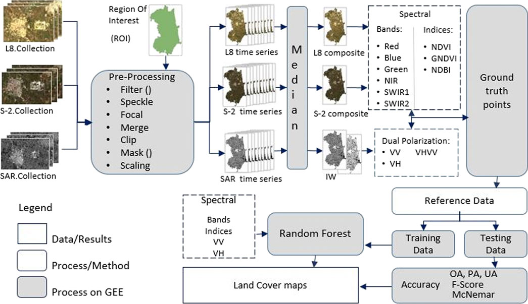
Figure 1. The workflow adopted for the land cover classification.

2.1 Study area

The study area is the Municipal territory of Acquaviva delle Fonti (40°53′N, 16°50′E). It is located in the province of Bari (Northern Puglia, Southeastern Italy) (Figure 2) and covers approximately 117 km².

Figure 2

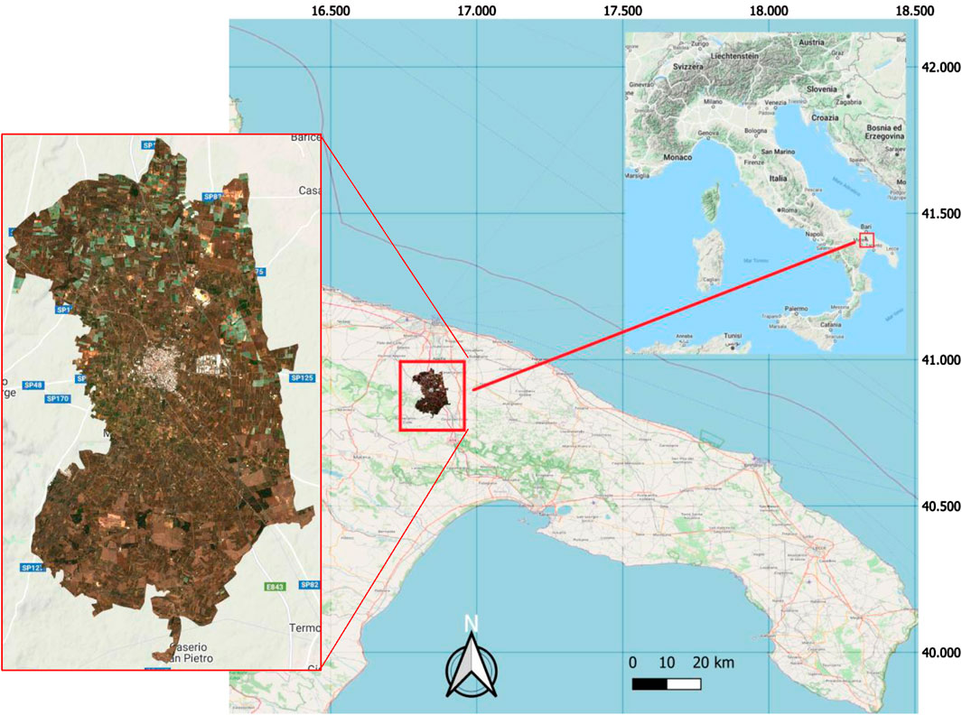
Figure 2. Study area (Open Street Map, 2023; Sentinel-2 RGB image, 2021).

The terrain is flat and lies in the hilly life zone with an elevation between 189 and 441 m above sea level. The climate is typically Mediterranean with warm, dry summers and mild, moist winters. The average annual temperature is 15.3°C and the average rainfall is 645 mm year⁻¹.

Eight land cover classes were identified after site inspections during spring of 2021. Cereals, mainly winter wheat, and vineyard under plastic films, constitute, respectively, the winter wheat and plastic films LULC classes. Other crops (crops in the rest of the article) was the class with the greatest extension and fragmentation. It mainly hosts legume and vegetable cultivations, olive and orchards. To a lesser degree, strips of oak (Quercus pubescens Willd. and Q. trojana Webb) and coniferous woods (Pinus halepensis Mill.) are found as forest. The municipality of Acquaviva delle Fonti and its industrial site fall within the investigated area as built-up. The mining activity (bare soil as land cover class) is limited to a site close to the urban center. A highway road also crosses the territory, as well as numerous photovoltaic fields.

2.2 Reference data collection

After identification of the land cover types which dominate the territory (Table 1, first column), a reference data collection (ground truth or training samples and validation samples) was created. The choice of reference dataset is an important step addressed at the best classification accuracy. The training dataset allows the selected classifier algorithm to learn the relationship between the pixel values of the various bands of composite/normalized indices/radar images and the land cover classes, with the aim of attaining optimal accuracy. The validation dataset allows to test the accuracy of the classifier.

Table 1

Table 1. Land cover classes and number of samples.

For these purposes, the training and validation dataset was designed combining imagery observation and field investigation. The reference dataset was determined using a random sampling approach, selecting the number of samples proportional to land cover classes surface (Table 1, second column), and taking into account the purity of samples (without mixed pixels).

To select the most homogenous pixel representative of every class and to reduce the effect of spatial autocorrelation, the reference samples were uploaded via GEE. Furthermore, data balancing technique, such as the augmentation of minority classes, was used to minimize class imbalance in the training dataset. Accurate visual analysis of Sentinel-2 RGB (2021) and Google Earth high-resolution (2018) images were employed to create reference samples. The assigned labeled classes were cross-checked by visually inspecting Google Earth imagery. The Google Earth images were used as a georeferenced base map to collect reference samples and to address field inspections, in case of inconsistencies between the visual information provided by the different images. In instances of uncertainty, class assignment was confirmed by checking normalized index values derived from optical images or visually inspecting ESA WorlCover maps (GEE image collection: ESA WorldCover v100 and v200; 2020, 2021). Moreover, samples with persistent high uncertainty underwent removal or were subject to field verification carried out in late spring 2021.

A total of 2492 reference samples were iteratively delineated for the period under consideration (Table 1). 80% of the randomly selected reference samples were used as training data, and the remaining 20% were used as validation data. Different data splitting approaches can be used to ensure a separation between the training and test data, including the holdout, the bootstrapping, and the cross-validation procedures. To avoid differences in accuracies, the same samples and split process were used to train and validate each dataset.

2.3 Cloud computing platform

Using multispectral/multi-source remote sensing data over large areas requires considerable technical expertise and high computational complexity (Shaharum et al., 2019). Those challenges can be effectively addressed by Google Earth Engine (http://earthengine.google.com), a cloud-based platform providing access to a multi-petabyte catalogue of Earth observation data, analysis algorithms and many other digital products (Padarian et al., 2015) that are ready-to-use with an explorer web app. It was designed to take advantage of Google’s computational infrastructure for planetary-scale access, storage, monitoring, analysis and visualization of geospatial data. An Application Programming Interface (API) enables users to create custom JavaScript and Python algorithms, while an associated web-based Interactive Development Environment (IDE), the Earth Engine Code Editor, provides high-speed parallel processing for prototyping, analysis and visualization of large-scale geospatial data (Gorelick et al., 2017; Tamiminia et al., 2020).

The GEE public data repository includes scientific datasets and several decades of historical images from multiple satellites. For this work, we used remote sensing data for which cloud computing and archived processed data in GEE had advantages for long time-series mapping, such as monitoring land type changes and detecting the extent of human settlement (Johansen et al., 2015). Moreover, machine-learning algorithms integrated into the GEE API allow short-time information extraction from satellite data, avoiding local memory consumption and intensive data transfers (Huang et al., 2017).

2.4 Remote sensing data

The remote sensing dataset consisted of 63 radar images and 16 optical images (Table 2) selected over the study area for the vegetative period 01/01/2021–31/05/2021. We used data from two optical sensors (Sentinel-2 MSI and Landsat 8 OLI) both to increase the number of optical images and to exploit the different bands resolution.

Table 2

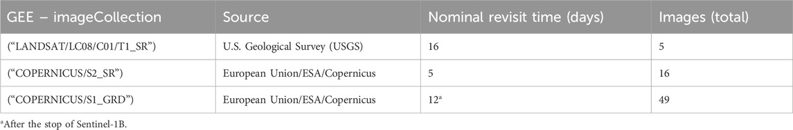
Table 2. Data source and descriptions.

The GEE cloud platform provides online access to a centralized catalogue of georeferenced and atmospherically corrected satellite multispectral images (Bunting et al., 2019), like the USGS and Copernicus archives that include Landsat 8 OLI/TIRS and Sentinel-2 (level 2A) data, respectively. We chose the atmospherically corrected surface reflectance scenes with the aim of minimizing the effects arising from the differences between satellite sensors (Landsat 8 and Sentinel-2) or the different acquisition dates. In addition, from the Copernicus collection, we selected the Sentinel-1 Synthetic Aperture Radar (SAR) (Table 2).

2.4.1 USGS Landsat 8

Landsat 8 acquires multispectral data from two sensor payloads, the Operational Land Imager (OLI) and the Thermal Infrared Sensor (TIRS), with a spatial resolution of 30 and 100 m, respectively. The OLI sensor collects nine narrower reflective wavelength bands in the visible (RGB), near-infrared (NIR), and shortwave infrared (SWIR) portions of the electromagnetic spectrum. Furthermore, the OLI sensor has two new spectral bands, a shorter wavelength blue band (B1 - Coastal Aerosol) and a shortwave infrared cirrus band (B9 - Cirrus). The TIRS detects land surface temperature and emissivity in two thermal bands (B10, B11).

2.4.2 Copernicus Sentinel-2

The Copernicus Sentinel-2 mission of the European Space Agency (ESA) comprises two polar-orbiting satellites (Sentinel-2A and Sentinel-2B), phased at 180° to each other, carrying an innovative high-resolution, multispectral imager (MSI), which provide a set of 13 spectral bands images from the visible to the shortwave infrared at 10–60 m spatial resolution (Romano et al., 2020), and a global absolute geolocation accuracy better than 6 m (ESA, Sentinel-2 User Handbook, 2015). The combination of a low revisit time (Table 2), wide swath coverage of 290 km, high-resolution spectral bands and novel spectral capabilities, make the Sentinel mission useful for a wide range of environmental applications (Immitzer et al., 2016). The Level-2A product, derived from the associated Level-1C and providing Bottom Of Atmosphere (BOA) surface reflectance images in cartographic geometry (ESA, Sentinel-2 User Handbook, 2015), was used in this study.

2.4.3 Copernicus Sentinel-1

Sentinel-1 is a remote imaging radar mission providing continuous day-and-night imagery, under almost all-weather conditions, with the C-band active sensor with an incidence angle between 20° and 45°. Data are acquired by the Synthetic Aperture Radar (SAR) in four imaging modes: Strip Map (SM), Interferometric Wide-swath (IW), Extra Wide-swath (EW) and Wave (WV) mode (ESA, SNAP - ESA Sentinel Application Platform, 2018). Following literature suggestion (Vizzari, 2022), the systematically distributed Ground Range Detected (GRD) Level 1 product was used in the Interferometric Wide-swath (IW) mode for the dual polarization VV + VH, depending on whether the radar signal transmitted in vertical polarization was received in vertical (VV) or horizontal (VH) polarization. The IW mode was selected since it is the operational mode over land. The dual polarization VV was chosen due to the stronger interaction of the vertically polarized electromagnetic field of the SAR with the vertical structures on the earth’s surface. The VH polarization was added to the first to intercept the changing orientation of territorial structures such as branches, roofs, plastic film covers, and streets.

We chose only scenes taken during the descending orbit so they were comparable in terms of backscatter intensity. The spatial resolution of Sentinel-1 was 10 m and is already available in GEE as an image collection. The final pixel size for the maps presented in this article was 10 m.

2.5 Normalized spectral indices

Several normalized spectral indices (NI(s)) have been proposed in the literature to extract the land cover types from remote sensing imagery. Data normalization has the advantage of reducing image noise when multi-sensor and multi-temporal images are used (Yang and Lo, 2002; Zurqani et al., 2018). Furthermore, these spectral indices could improve image classification accuracy, thereby emphasizing the detection of vegetation reflectance signatures or reducing hill shade and building shadows. Supplementary Figure S1 shows a Sentinel-2 derived NDVI time series for the eight land cover classes detected in the study area. Winter wheat had one NDVI peak in 2021 indicating one harvest per year. Deciduous oaks (Quercus trojana Webb. and Q. pubescens Willd.) have a growing stage in spring after the new foliage. Coniferous trees (Pinus halepensis Mill. and P. pinea L.) show a somewhat varying index, such as the urban dwelling. This illustrated the importance of using seasonal information to discriminate vegetation covers from infrastructures.

Some of the standardized indices are sensitive to different factors related to seasonality, study area location, and image resolution. However, given their simplicity and easy formulation, such methods have been widely used for LULC monitoring and mapping.

In this study, the normalized indices calculated from the composite bands of Sentinel-2 and Landsat 8 imagery, and Sentinel-1 imagery are reported in Table 3:

Table 3

Table 3. Formulation of the satellite-derived standardized indices.

The Normalized Difference Vegetation Index (NDVI) (Rouse et al., 1974) is an index of the vegetation greenness that derives from measurements of the optical reflectance of sunlight in the red and near-infrared wavelengths. It is not a physical property of the biome’s cover, but its very simple implementation makes it widely used for ecosystem monitoring (https://land.copernicus.eu/global/products/ndvi). NDVI is suitable for estimating leaves’ vigor during the early vegetative stages.

The Green Normalized Difference Vegetation Index (GNDVI) (Gitelson et al., 1996) is more sensitive than NDVI to the proportion of chlorophyll absorbed radiation since the Red band is replaced in the calculation by the Green band. It is used to assess photosynthetic activity, water content, and nitrogen concentration in more advanced development stages of dense plant canopies (Vizzari, 2022).

Most of the normalized vegetation indices confuse built-up with bare soil surfaces (Valdiviezo et al., 2018); to reduce such limitations, a built-up index was used in this work.

The Normalized Difference Built-up Index (NDBI) (Zha et al., 2003) uses increased reflectance values from SWIR and NIR bands to highlight manufactured built-up areas. In thermal infrared bands, the higher emissivity and albedo of built-up structures, compared to bare soil, waterbodies, and vegetation, is best detected by this index (Ali and Nayyar, 2021). It is based on separating the built-up area from the background and mitigating the effects of terrain illumination as well as atmospheric effects. According to this index, the greater the value of a pixel in the derived image, the higher the possibility of the pixel being a built-up surface (He et al., 2010).

2.6 Datasets for land cover classification

To analyze the multispectral data combinations on the land cover classification process, we aggregated optical data, radar data and spectral normalized indices into five different input data and combined these data in thirteen different datasets, seven without NI(s) and six with NI(s) (Table 4).

Table 4

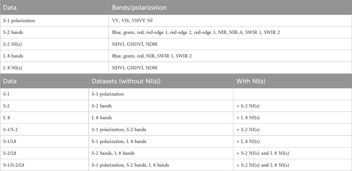
Table 4. Data source, descriptions and datasets.

2.7 Processing method

The workflow of the methodological approach adopted in this study for land cover classification is reported in the Graphical abstract. First, the Copernicus (i.e., Sentinel-2 and Sentinel-1) and Landsat 8 image collections comprising the Region of Interest (ROI) were selected via GEE. The winter-spring period of 2021 was chosen to distinguish winter wheat from bare soil land cover. The selected collection data were then processed with GEE to manually detect the main land types in the study area and generate training and testing data. The Random Forest (RF) classifier was then used to generate the LULC map. Lastly, a validation step and an accuracy assessment were performed before the digital restitution of the final land cover map for the study period. The detailed methodology is described in the following paragraphs.

2.7.1 Imagery pre-processing

The land cover detection technique requires image pre-processing and normalization. In this step, we used the GEE API to develop a time series of calibrated remote sensing images from January to May 2021. A double process of filtering the satellite image collections by the period and intersecting the boundaries of the study area was performed, using a specific script in GEE, to develop the time series. Additional filtering was applied to radar images to refine the selection based on Instrument Mode, Polarization, and Orbit properties. Since it was not possible to get a continuous, cloud-free time series for optical data, a five-monthly composite image was composed to ensure a cloud-free time series for the whole investigated area. A cloud filter was preliminarily applied to remove the image pixels with >10% cloud contamination. All the images selected were then processed and analyzed for masking out the remain pixels containing various types of clouds, snow, ice, haze, and quality disturbance. A custom cloud-masking and compositing JavaScript were used to produce a per-pixel, cloud-free, multispectral image of the study area. The script uses a quality flag band, QA for Landsat 8, and QA60 for Sentinel-2, to identify and mask out flagged cloud and cloud shadow pixels. For Sentinel-2, the remaining cloud and aerosols were identified and masked using the scene classification (SLC) band provided in the Sentinel-2 Level 2A product to mask out cirrus and aerosol bands. A scaling function was implemented to switch from Landsat Collection 1 to Collection 2 data.

The pre-processing steps for the SAR images (apply orbit file, backscatter mosaics, border noise removal, thermal noise removal, terrain correction, and radiometric calibration), as implemented in the Sentinel Application Platform (SNAP) Toolbox (ESA, SNAP - ESA Sentinel Application Platform, 2018), were already performed by GEE after S-1 data ingestion. Speckle filtering was applied to reduce speckle effects (Mullissa et al., 2021).

All the preprocessing script used in this study are available in the GEE API Reference (https://developers.google.com/earth-engine/apidocs).

2.7.2 Composite image

The optical images, making up the seasonal time series, were taken during the growing season with the most abundant leafage and correspond to the vegetation greenness peak driven by the warm and moist season conditions. This selection aligns with the observation requirements necessary for detecting natural and human-induced land cover (Table 2).

A median composite approach was performed to generate a representative seasonal image. Specifically, the median value was computed for each spectral band to minimize the influence of outliers and residual noise. The method follows the best-available pixel compositing approach introduced by White et al. (2014), which is widely used in remote sensing to reduce the amount of invalid pixels after pre-processing and to ensure consistency in the final composite (Bey et al., 2020). Although multiple statistical methods could be executable for compositing, the median index was chosen as the best response for this analysis. The median composite approach is frequently applied in geospatial analyses involving multi-temporal datasets, as it reduces the impact of atmospheric variability and sensor noise more effectively than the mean (Bunting et al., 2019).

2.7.3 Random forest (RF) classifier

In this study, the classifications were performed using a pixel-based supervised RF classifier consisting of an ensemble of decision trees (Zurqani et al., 2018; Ghorbanian et al., 2020). RF is widely regarded as one of the most robust machine learning algorithms for land cover classification and is increasingly used in classifying remote sensing data (Teluguntla et al., 2018). In particular, RF was chosen because of the high accuracy with multi-source datasets and ability to handle diverse input datasets (Phan et al., 2020). An RF algorithm requires the setting of several parameters, with the most critical being: 1) the number of decision trees (ntree), which determines the ensemble size in the run and influences the classification stability; 2) the number of randomly sampled variables as candidates at each split (mtry), controlling the diversity of trees in the ensemble and preventing overfitting (Immitzer et al., 2016). Based on the recommendations from several studies, reported by Phan et al. (2020), we used the default model parameters, which also proved to be the best performing in this work. Specifically, the model was trained with 500 trees, while the number of the variables per split was set to the square root of the total number of samples in each class.

For the training step of the RF machine-learning algorithm, an iterative sample selection procedure (Teluguntla et al., 2018) was implemented o refine the training dataset and improve classification accuracy. The RF classifier was built using an initial training sample dataset within the GEE platform. Then, both the training and validation datasets were iteratively adjusted until an optimal classification and accuracy outcome were achieved. To ensure reliability, the classification results were visually compared to high-resolution images from Google Earth. Furthermore, ground-truth samples or visual assessments of historical satellite imagery were performed for cases of hard interpretation. Having acquired a high level of accuracy, the validation step was performed using the independent validation dataset, ensuring that test samples were not used in training. The classification was accepted after the Overall Accuracy indices derived from the confusion matrix were, for validation dataset, adequately high (80%), confirming a high level of classification reliability.

2.8 Accuracy evaluation

The RF algorithm performance in correctly classifying a random set of features (sample points) was measured by the accuracy of the fourteen classification maps produced. Therefore, once a classification was run, the accuracy of the process was determined. As explained in Section 2.2, each of the land cover map produced was then validated using a dataset obtained from 20% of the total reference locations, via GEE. To ensure the separation between train and test data, we used the cross-validation procedure, in which each sample is included exactly once in the test set and each sample in the test is not used to train the classifier. The optimal tuning parameters percent distribution was determined based on multiple percent distribution of training data to evaluate the effects of different parameter configurations on the performance of the classifier. The definitive classification dataset created for this purpose includes samples randomly selected for each land cover type. The cross-validation comparison produces a table, the confusion matrix, which contains the number of pixels classified correctly or incorrectly in each class. The matrix allows the computation of several accuracy metrics: Overall Accuracy (OA), measuring the proportion of correctly classified pixels; Producer’s accuracy (PA), evaluating how well reference (ground-truth) samples were classified; User’s accuracy (UA), assessessing classification reliability from a user perspective. The goal is to obtain not just the higher OA, but also a good balance of PA and UA, ensuring that classification performance was not biased toward dominant land cover types. To depict the balance of PA and UA, the F-score was calculated as a harmonic mean of PA and UA (Sokolova et al., 2006).

The McNemar’s statistical test (McNemar, 1947) was applied as an additional measure to compare the significance of difference between classification results, with p-values lower than 0.05 regarded as significant.

The kappa coefficient (K) was deliberately excluded because its use was recently discouraged in assessing land cover classification accuracy (Foody, 2020).

Lastly a variable importance analysis was performed for all spectral bands and indices, providing insights into which features contributed most to the classification model. The result paragraph are reported in Section 3.3.

3 Results

The land cover classification maps were produced from remote sensing images using the Random Forest supervised classifier, in a total of eight land cover classes. Besides the single sensor RF-classification, using Sentinel-2, Landsat 8, SAR satellite images and their combination, additional variables such as normalized Indices were used both to map land cover then to assess how they increase or decrease the accuracy of the results.

An aggregated sample of the land cover classes surface is shown in Figure 3. It illustrates that the majority of variations in the land cover surface occurred after SAR processing, with the exception of the classes characterized by the highest NDVI values such as winter wheat, crops, and forest. The predominant land cover class was crops, encompassing an average area of 73.38 km², which constituted 62.29% of the total study area. The data without NI(s) were very similar in area for each dataset.

Figure 3

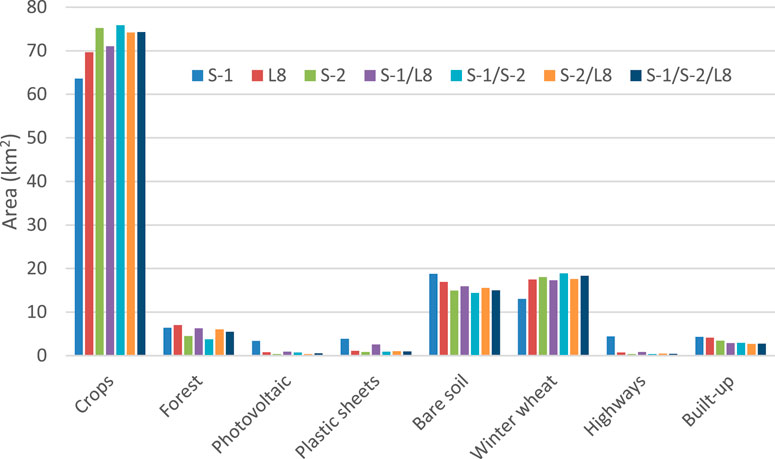
Figure 3. Acquaviva delle Fonti Municipal territory. Land cover classes surface derived from classification of satellite images and NI(s).

3.1 Accuracy

Based on a dataset collection of 1,980 training samples and 512 validation samples, for 2,492 reference samples (Table 1), the accuracy of classifications was characterized by the Overall Accuracy (OA) always above 0.7773, except for S-1 data where the accuracy score was 0.613 (Figure 4; Table 5). The numeric values of Overall Accuracies index reported in Table 5, whose bar chart is displayed in Figure 4, provide a significant insight into the overall contribution of multi-sensor imagery to the LULC classification quality. Also, Figure 4 shows the F-score graphic bars.

Figure 4

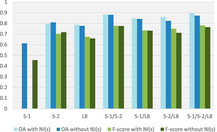
Figure 4. Classification accuracy (OA, Overall Accuracy; F-score = harmonic mean of PA and UA, NI(s), normalized spectral indices).

Table 5

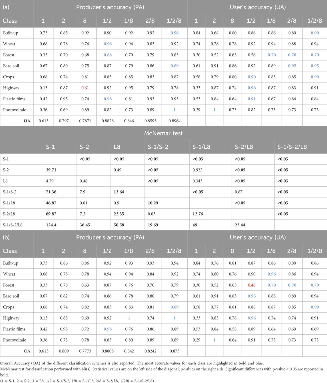
Table 5. Class Producer’s and User’s accuracies of the different classification schemes with Normalized indices (a) and without Normalized indices (b).

OA increases from radar to optical images and with the decreasing of the image pixel size (from Landsat OLI to Sentinel-2). For classifications obtained using spectral indices, the combination of the satellite imagery slightly increases the statistical metrics, with the exception of S-2, which shows an inverse trend, decreasing OA with NI(s) (Table 5; Figure 4). The dataset that combined the complete satellite imagery (S-1/S-2/L8) and NI(s) computation, achieved the highest accuracy with OA = 0.8964 (Table 5a) and F-score = 0.7806, followed by the dataset combining the Copernicus sensor data with NI(s), where OA = 0.8828 (Table 5a) and F-score = 0.7768. In the investigated period, the cumulative number of images used demonstrated that a combination of Landsat OLI, Sentinel-1, and Sentinel-2 performed better than a single sensor. The accuracy increases with the increasing number of bands used. The results illustrated in Figure 4 and Tables 5a, b show that Sentinel-2 always had better accuracy than Landsat 8.

Graphic and numeric reports of accuracy metrics do not hold information on the classification of individual land cover classes. Exhaustive details on LULC classes accuracies can be seen in Table 5, reporting the Producer’s accuracy (PA), a percent index that synthesizes the probability that a certain land cover on the ground has been correctly classified on the map produced, and the User’s accuracy (UA), the ratio between the correctly classified sites and the total number of classified sites.

PA and UA accuracies, with the exception of S-1, range between 0.61–1 and 0.48–1, respectively. The lowest Producer’s accuracy was observed for highway class (0.61), after L8 classification with NI(s), and the lowest User’s accuracy for forest (0.48), after S-1/S-2 classifications without NI(s).

Table 5 shows that the highway class was mapped with the highest PA (1) when the classification was based on S-1/L 8 and S-1/S-2/L 8 scenes without Ni(s). The highest PA and UA (1) were performed for the photovoltaic class using, respectively, S-1/S-2/L8 with NI(s) and S-2. High values of PA (0.98) was calculated for the plastic film class with Copernicus data combinations.

Although the use of normalized indices slightly increases the Overall Accuracy of classification, except for S-2 (Table 5; Figure 4), some deviations can be observed for the individual land cover types. The crops type, which was the predominant class, took advantage from using the complete set of optical and radar data when producer and user accuracies, for that class, were 87% and 90%, respectively. Built-up was better detected by the combination of radar and optical data (with NI(s)), both for PA and UA perspective. Forest and bare soil classes show the highest UA for classification performed combining all sensors dataset and normalized indices. Winter wheat PA best results were performed after the combination of Copernicus (S-1/S-2) datasets and NI(s). Photovoltaic class reaches the highest UA scores (1) for S-2 dataset, both with or without adding NI(s). The highest PA score of bare soil class (0.89) was achieved for S-1/S-2/L8 combination with NI(s), while the highest UA (0.95) was performed several times: combining both optical data (S-2/L 8) or radar and optical data (S-1/S-2/L 8) with NI(s), combining Copernicus data without NI(s).

The statistical significance of the difference in OA between the classifications performed with NI(s) was assessed using the McNemar test, with p < 0.05 (Table 5).

Matrix of McNemar test showing the statistical significance of differences between every classification pairs. The McNemar test revealed that the difference between the classification using the S-1/S-2/L8 and S-1 datasets were always statistically significant (p-value <0.05) in every comparison. Lesser values of significance were assessed for S-2/L8 when compared with S-1/S-2. Moreover, the higher value of significance was detected between S-2 and S-1/L8 classification (p-value = 0.922).

For the most accurate classifications (S-1/S-2/L8 and S-1/S-2), the accuracy of each land cover class was compared, both considering NI(s) (Figure 5). Differences in the producer’s accuracies between the quoted datasets were less than 6.25 for all classes, except for the photovoltaic and highway class, whose PA differences were 18% and −17.95%, respectively. Differences in the User’s accuracies were less than 8.35% for all classes, except for the photovoltaic and forest classes, whose UA differences were −12.33% and 20%, respectively.

Figure 5

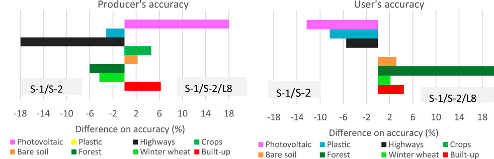
Figure 5. Difference in classification accuracy between Sentinel-1/Sentinel-2/Landsat 8 and Sentinel-1/Sentinel-2 for each land cover class, both with normalized indices. The negative values represent a higher accuracy for the S-1/S-2 dataset.

In both land cover classifications, crops had the same UA value, so the percentage difference accuracy was equal to zero and does not appear in the UA chart (Figure 5). Built-up, bare soils, and crops, were more accurately classified with the complete combination of radar and optical datasets. Plastic films and highway classes were better classified with the Copernicus dataset combination.

3.2 Classification maps

Figure 6 shows the LULC classification maps on three example sites (A, B and C), performed with Sentinel-2 multispectral data (row 1), Sentinel-2 data combined with L 8 (row 2), with S-1 (row 3), and with S-1/L 8 (row 4), all with NI(s). The classified maps are graphically very similar for each inset. Border pixels between adjoining class types often show different boundaries drawn depending on the different spatial resolutions of source images and spectral contamination of pixels near field edges.

Figure 6

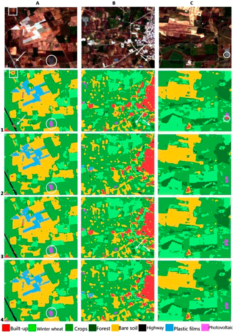
Figure 6. Comparison of three example sites (A–C) with S-2 (1), S-2/L 8 (2), S-2/S-1 (3) and S-2/S-1/L 8 (4) land cover classifications (Spatial resolution 10 m).

A heterogeneous area with agricultural crops, bare soils, plastic film covers, photovoltaic fields, and a highway is displayed in (Figure 6A). All the classified maps detect the photovoltaic field well, highlighted by the white circle, as well as the plastic films, represented in light blue. The bare soil areas are correctly mapped by every satellite combination. With S-2 classification (Figure 6 A1), a bridge over the highway (with a white arrow) and an area inside bare soil land (white square), were wrongly classified as built-up classes. The multispectral combination between S-2/L 8 (Figure 6 A2) and S-2/S-1/L 8 (Figure 6 A4) showed an increase of visual accuracy.

An urban area with its surrounding agricultural fields and bare soil is displayed in (Figure 6B). The confusion of built-up class (Figure 6 B1) was progressively reduced by the addition of a single Landsat 8 (Figure 6 B2) or Sentinel-1 data (Figure 6 B3) to Sentinel-2. Further reduction was performed by the addition of radar (Figure 6 B4) to optical combination. This reduced confusion can be seen directly in the confusion matrices for the whole municipal territory mapped (Table 6). High-density plantations (white arrows) were classified as forests instead of crops in S-2 and S-2/S-1 maps (Figure 6 B1 and B3). S-2/L 8 (Figure 6 B2) and S-2/S-1/L 8 (Figure 6 B4) were instead more accurate.

Table 6

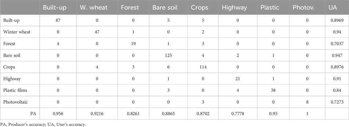
Table 6. Confusion matrix of the RF validation samples performed for S-1/S-2/L8 band combination and NI(s).

A less heterogeneous agricultural landscape, with crops, winter wheat, bare soil, and forest covers, is represented in Figure 6C. Land cover stands were well detected from every satellite single sensor or multispectral combination. A misclassifying of built-up instead of photovoltaic class was observed (white circle) in the Sentinel-2 derived map (Figure 6 C1). Here, each multispectral combination considered showed an improvement of accuracy respect to the use of S-2 (Figure 6 C2–C4).

In all the maps produced, an incorrect classification of built-up as bare soil or crops can be attributed to the diffuse presence, in several sites of the investigated territory, of outcropping rock.

Figure 7 displays the LULC classification of the whole territory of Acquaviva delle Fonti performed using S-1/S-2/L 8 band combination, with normalized indices. The detailed insets (Figure 7) and the whole territory classifications (Figure 7) demonstrate a surprisingly smooth result of the classified LULC, given that no prior segmentation technique was applied.

Figure 7

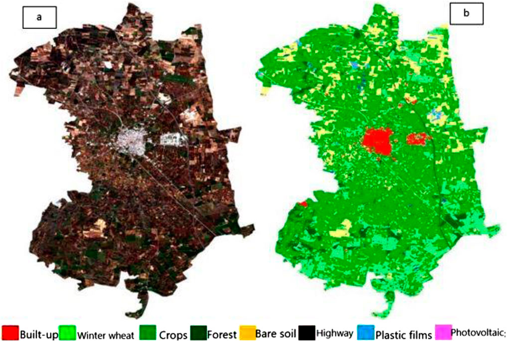
Figure 7. Sentinel-2 satellite image (a) and pixel-based Acquaviva municipality maps (b) with a 10 m classification map produced using GEE for optical (Sentinel-2, Landsat 8) and radar (Sentinel-1) data.

3.3 Feature importance

The large amount of multi-source input predictors data required a detailed assessment of single band importance for classification efforts. Figure 8 displays the Gini importance (Breiman et al., 1984), as standardized values, of the input features used for LULC classification. This variable gives quantitative information about the contribution of different bands to the Random Forest classifier used. A specific predictor plays a significant role in the classification when associated with a high Gini importance; instead, a low importance means that a specific feature determines only limited improvements.

Figure 8

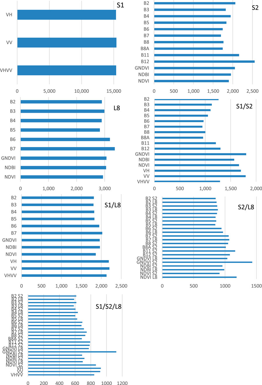
Figure 8. Spectral datasets: bands and NI(s) variable importance. (L8 = Landsat 8, S1 = Sentinel-1, S2 = Sentinel-2).

For Sentinel-2 image (S-2), short wave infrared 2 band (B12) was the highest performing band, fully in line with other studies (Schuster et al., 2012; Immitzer et al., 2016), while red edge 3 band did not perform as well.

The near infrared band (B5) was the variable with less importance in Landsat 8 classification, both as a single sensor and combined with Sentinel-2 data (S-1/L 8 and S-2/L8). For the S-1/L 8 bands combination, vertical visualization (VV) of C radar data was the band with the higher contribution to detect LULC types of investigated territory. The Sentinel-2 green band (B3) did not perform as well for all optical and radar data combinations (S-1/S-2/L 8).

The importance of the normalized difference indices was quite different in the classifications performed. Green Normalized Difference Vegetation Index (GNDVI) was the higher performing band in optical combination (S-2/L8), even in combination with radar data (S-1/S-2/L8).

Focusing on visible bands, it appears (Figure 8) that those bands were unimportant in the Landsat OLI single sensor classification (L8) and in all the classifications performed in combination with that sensor data (S-1/L 8, S-2/L 8, and S-1/S-2/L 8), where the visible bands of the Sentinel-2 sensor also did not perform as well.

For Sentinel-1 image, VV band performed a variable importance slightly higher than VH band or VH and VV bands combination.

4 Discussion

In this work, we provided a versatile framework for LULC mapping and evaluated its effectiveness in mapping a heterogeneous territory in southern Italy. The resulting land cover map has practical applications in Italian territory, serving as valuable input for decision support to aid in planning and management, investigating opportunities for agricultural expansion and environmental needs.

The combined use of the Random Forest (RF) machine learning algorithms and cloud platforms, such as Google Earth Engine (GEE), confirmed to be useful tools for analyzing and processing geospatial big data (Phan et al., 2020; Tassi et al., 2021; Sidhu et al., 2018; Zurqani et al., 2018; Vizzari, 2022) and obtaining higher accuracy in the pixel-based classification methodology (Wieland and Pittore, 2014; Pan et al., 2022; Trujillo-Jiménez et al., 2022). To further increase the accuracy of the results a data combination methodology was adopted (Ye et al., 2014; Quan et al., 2020). Specifically, single sensor data (S-1, S-2, L8) and different sensor data combinations (S-1/S-2, S-1/L 8, S-2/L 8, S-1/S-2/L 8) were tested in the study area. Moreover, three normalized spectral indices (NDVI, GNDVI, NDBI) and a radar index (VHVV) were also used to better emphasize vegetation reflectance signatures or reduce hill shade and building shadows.

A statistical assessment of the results obtained was carried out using splitted validation samples (Quan et al., 2020; Lanorte et al., 2017; Chen et al., 2017), to verify the reliability of the final, pixel-based LULC maps produced and to compare the accuracies of different multi spectral/multi source datasets in land cover classifying. Despite large areas of the territory being covered with a heterogeneous mix of crops (legumes, vegetable, olive, orchards), vegetation habitats and built-up settlements, and the complex mix of transitions between different land cover types, Overall Accuracy >80%, for a seasonally aggregated composite dataset, was generally achieved.

We used indices and bands together because the datasets using the NI(s)-only predictors obtained lower levels of accuracy than the datasets using reflectance measurements. Although the spectral indices are a useful way of analyzing vegetation covers or urban settlements (Fan and Liu, 2016) and were successfully used in the past, NDVI, GNDVI and NDBI did not work well alone as full descriptors of optical imagery in characterizing a large variety of LULC classes of the investigated territory. This could be due to the reduction of the spectral bands processed to detect land cover when those indices were used alone. Indeed, Yu et al. (2014) found a positive linear correlation between the number of bands used in classification and the classification accuracy for different, multi-sensor dataset types.

The datasets that combined optical and/or radar data with the normalized difference indices (NDVI, GNDVI, NDBI, VHVV) were the most accurate (Zurqani et al., 2018; Vizzari, 2022; Quan et al., 2020). The OA of the LULC classifications was significantly high, reaching 0.8964, for the S-1/S-2/L8 data combination (Table 5).

The Sentinel-2 single-sensor datasets obtained higher accuracy than Landsat 8 single-sensor datasets, with the OA about 80%. The combined multi-sensor datasets obtained the most accurate LULC classifications. The combination of Copernicus data with normalized indices produced levels of accuracy only lower than those obtained combining optical and radar data (S-1/S-2/L 8/).

The Sentinel-1 datasets obtained the worst accuracies (Table 5; Figure 4). However, this work revealed the C band capability to slightly improve the optically derived classifications based on the high radar image frequency and the different polarization (Ye et al., 2014; Quan et al., 2020). Winter wheat, crops, and built-up classes experience advantages with the addition of SAR imagery, benefiting both producer’s (PA) and user’s (UA) accuracies. In the case of built-up areas, only the PA of the S-1/L8 combination, accompanied by normalized indices (NI), remains unchanged. The classification of plastic films exhibits a notable enhancement when C-bands are introduced to optical imagery, except for the S1/S2/L8 combination, where UA remains unaffected.

Table 7 summarizes the qualitative variations, from producer’s and user’s perspective, performed by optical dataset after adding Sentinel-1 data.

Table 7

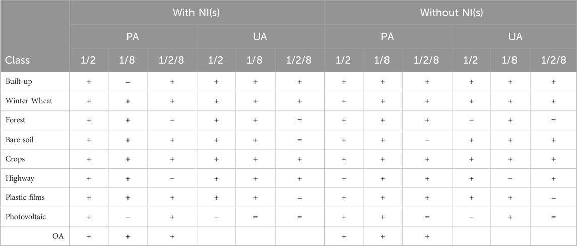
Table 7. Qualitative variation of land cover classification after adding SAR data.

The RF supervised classification accurately delineates the urban and industrial settlements, a hospital area, and nearly the individual buildings scattered throughout the territory (Figure 7). The anthropic interventions such as plastic films, used for vineyard crop protection, and photovoltaic fields were correctly delineated (Malof et al., 2016; Sun et al., 2021). Moreover, the highway was accurately distinguished and good capability in discriminating crops, winter wheat, and bare soil classes was observed (Tran et al., 2022). Visually, the most accurate pixel-based LULC final map of the study area (Figure 7b), based on visual interpretation and comparison with the Sentinel-2 composite satellite image (Figure 7a), is noiseless and well-defined. In line with the Löw et al. (2013) findings, the number of RF decision trees was set to a relatively high number of 500, after testing the importance of this parameter by changing it, whereas other parameters were set the same.

A confusion matrix was generated to assess misclassification errors in land cover classification. Several factors contributed to misclassification, including mixed pixels in heterogeneous landscapes, spectral similarities between different classes, differences in spatial resolution among sensors, algorithmic constraints, and atmospheric interference. Additionally, variations in land cover phenology may have led to temporal inconsistencies, particularly in classes with seasonal vegetation.

From the confusion matrix (Table 6), it became apparent that specific confusion occurred between built-up and bare soil or crops (Bhatti and Tripathi, 2014). The irregular presence, in the study area, of un-vegetated outcropping bedrocks, which the satellite sensors detect as built-up structures may have generated this issue. Forest was well classified, even taking into account the confusion with the built-up class due to the urban parks. Highway and winter wheat had the lowest degrees of misinterpretation, while bare soil and crops had the highest ones due to their territorial heterogeneity. Some photovoltaic panels present in crops generated confusion between these classes.

The key to obtaining satisfactory classification results is the quality of the reference data selected (Congalton et al., 2014). In this work, both the training and the validation samples were kept constant for each input dataset, while the ground true points control was based on visual interpretation of high-resolution satellite images or, in case of misinterpretation, after in situ recognition. Several studies have obtained high classification accuracy in territories less heterogeneous than the Acquaviva municipality, characterized by few land cover classes more easily detected by a remote sensing approach, due to their almost univocal spectral signature (Carrasco et al., 2019).

In summary, the GEE platform enabled high-speed analysis of a large dataset freely available for research, using parallel processing on remote servers that allowed the combination of data from multiple sensors without the preliminary finding and downloading steps. Furthermore, the GEE routines can combine optical images to detect the best cloud-free pixels to create full cloud-free images (Kumar and Mutanga, 2018); this was a helpful approach, in this work, to assess a great number of images for accurate classification and provided an acceptable representation of all LULC classes (Tamiminia et al., 2020; Shafizadeh-Moghadam et al., 2021).

The RF supervised classification provides flexibility in the modeling process for combining multi-source data types with the aim of accurately classifying the territory of Acquaviva delle Fonti. Particularly, this study shows the potential of the combined use of optical and radar imagery for LULC classification of agricultural areas characterized by a heterogeneous land cover. Unlike the case of landscapes with clearly distinguishable land cover categories such as water, forest, bare soil, and built-up areas, here the LULC types were numerous and very fragmented, even within the individual classes. The forest type includes both coniferous and broadleaf trees. The latter, mainly deciduous oaks, can be easily misclassified as fruit trees, just like the fruit trees of the crops class. Crops, the class with the largest surface, was indeed characterized by various combinations of agricultural crops differently organized: fruit trees (Cherry, Almond, Olive, etc.) over annual crops (legumes, vegetables), annual crops without fruit trees and vice versa. Plastic films were of different colors and shape, sometimes completely covering the soil and sometime partially. The performed classifications seem overcome the misclassification errors, detecting with an appropriate accuracy the LULC stands.

Finally, this work, confirmed that increasing the number of bands leads to a greater ability to capture complementary information on the spectral and structural characteristics of land cover types. Data combination is an effective methodology which could improve the accuracy of the results (Ye et al., 2014; Quan et al., 2020) especially considering heterogeneous landscape.

In addition to assessing the effectiveness of combining radar and optical data on land cover mapping, the methodological contribution of this study also concerns the following topics: Time period selection; Multi-temporal remote sensing data; Median composite approach; Supervised pixel selection; Random Forest classifier; Training and validation dataset; Cross-validation of classification; Variable importance analysis; Multiple accuracy assessment (OA, PA, UA, and F-score); Statistical significance (McNemar’s test); High accuracy threshold (≥80%).

The increasing accuracy of the results could also improved by detecting land features at different times (Lopes et al., 2020) and could be the subject of future studies such as area estimation and accuracy assessment of land change by using Olofsson et al. (2013); Olofsson et al. (2014) procedure. To mitigate misclassification, future work could apply post-classification refinement techniques such as majority filtering. Another suggestion for future works involves the object-based approach integrated with the Gray-Level Co-occurrence Matrix (GLCM) to extract textural index statistics and applying Simple Non-Iterative Clustering (SNIC) to identify spatial clusters.

5 Conclusion

The LULC classification of the complex environment by means of remote sensing images is challenging due to the extreme fragmentation of the different land uses such as rural buildings, roads, plastic films (Hurskainen et al., 2019). Another issue is represented by the huge amount of data which needs high-powered processing resources (Scheip and Wegmann, 2021; Amani et al., 2020).

This study has analyzed the potential of multi-sensor imagery and normalized derived indices to characterize and detect LULC in small-scale areas dominated by heterogeneous land use and frequent cloud cover. Using S-1, S-2, and L8 imagery for land cover mapping, the accuracy of single-sensor dataset versus multi-sensor dataset was provided.

The results indicate that optical and radar data combination (S-1/S-2/L 8) approach performed higher LULC overall classification accuracy (OA) than a single-sensor (S-1; S-2; L 8) approach and when normalized spectral indices were added to the combination.

Datasets only based on SAR images performed the lowest accuracy levels, whereas combined datasets (S-1/S-2/L8 or S-2/L8) outperformed one-sensor datasets.

The pixel-based classification, performed using the complete dataset combination with an RF classifier, achieved the highest Overall Accuracy score of 89.64%. The most accurately classified land cover classes were photovoltaic, plastic films, built-up, and winter wheat with producer’s accuracies higher than 96% and all class-specific accuracies (PA and UA) were generally higher than 75%.

Pixel-based image analysis faces some limitations. Firstly, image pixels do not perfectly represent real geographical objects, and their topology is constrained. Secondly, this approach tends to overlook spatial photo-interpretive elements like texture, context, and shape. Lastly, the heightened variability present in high spatial resolution imagery can confound pixel-based classifiers, leading to reduced classification accuracies.

Enhancing classification accuracy commonly involves augmenting the number of training samples. Nonetheless, users are constrained to utilize only a specific quantity of samples within classification methods (Vuolo et al., 2018).

Despite data processing and classification limitations, the integration of optical (Sentinel-2 and Landsat 8) and SAR (Sentinel-1) data captures complementary information on the spectral and structural characteristics of land cover types. In general, a higher number of bands resulted in a higher level of classification accuracy. The framework presented in this study, will of interest to improve land cover dynamic studies, such as hydrological modeling or land consumption in complex and fragmented environments along all the regional and national territory.

Data availability statement

The original contributions presented in the study are included in the article/Supplementary Material, further inquiries can be directed to the corresponding author.

Author contributions

GRo: Conceptualization, Data curation, Investigation, Methodology, Software, Supervision, Writing – original draft, Writing – review and editing. GRi: Supervision, Writing – review and editing. FG: Writing – review and editing, Formal Analysis.

Funding

The author(s) declare that financial support was received for the research and/or publication of this article. The research activity was financed by Civil Protection - Puglia Region program “INTERREG ipa cbc Italia-Albania-Montenegro: Project To Be Ready.”

Conflict of interest

The authors declare that the research was conducted in the absence of any commercial or financial relationships that could be construed as a potential conflict of interest.

Generative AI statement

The author(s) declare that no Generative AI was used in the creation of this manuscript.

Publisher’s note

All claims expressed in this article are solely those of the authors and do not necessarily represent those of their affiliated organizations, or those of the publisher, the editors and the reviewers. Any product that may be evaluated in this article, or claim that may be made by its manufacturer, is not guaranteed or endorsed by the publisher.

Supplementary material

The Supplementary Material for this article can be found online at: https://www.frontiersin.org/articles/10.3389/frsen.2025.1535418/full#supplementary-material

References

Ali, A., and Nayyar, Z. A. (2021). A modified built-up index (MBI) for automatic urban area extraction from landsat 8 imagery. Infrared Phys. Technol. 116, 103769. doi:10.1016/j.infrared.2021.103769