Non-stereotypy (to species) in mysticete downsweeps

The Australian EEZ provides habitat for ten species of mysticete whales seasonally supporting critical life functions ranging from feeding to breeding. All of these species produce downsweeping calls, which may confound passive acoustic monitoring efforts. In an attempt to optimize a detector for Eastern Indian Ocean pygmy blue whale (EIOPBW) downsweeps, we tried a spectrogram correlator based on confirmed templates and a neural network trained on general blue whale D-calls followed by clustering algorithms. Outputs were manually validated by bioacousticians. We found that downsweeps exhibit significant variability and form a graded continuum of acoustic features, as opposed to clusters. Comparative analysis demonstrated parallels between EIOPBW call variants and downsweeps of other mysticete species, raising concerns about the reliability of assigning calls to species based solely on spectrographic features. Geographical and seasonal patterns of downsweeps were more conclusive for EIOPBW when aligned with known migratory routes and timings. Challenges in automated detection, variability in environmental noise, and human biases in manual classification were acknowledged. To improve species identification, we suggest integrating soft labeling, advanced acoustic transforms, sound propagation corrections, and cross-referenced databases. Until automated methods achieve higher reliability, passive acoustic monitoring will require a multidisciplinary approach incorporating regional ecological insights and manual validation.

1 Introduction

With the world’s third largest exclusive economic zone (EEZ), Australia has strategically developed its blue economy over the past decade, comprising shipping (ship building and port expansion), offshore energy (oil, gas, and renewables), tourism, fisheries, and aquaculture (Australian Government, 2013). Western Australia, in particular, has a strong history of offshore energy development, ranging from oil and gas off the northwest coast to upcoming windfarms off the southwest coast^1,2. Moreover, the growth of Western Australian ports is planned for both shipping and maritime defense^3,4. Sustainability of the blue economy hinges on careful environmental planning to safeguard Western Australia’s marine biodiversity.

The Western Australian offshore environment provides habitat to ten species of baleen whale: common minke whale (Balaenoptera acutorostrata), Antarctic minke whale (B. bonaerensis), sei whale (B. borealis), Bryde’s whale (B. edeni), blue whale (B. musculus), Omura’s whale (B. omurai), fin whale (B. physalus), pygmy right whale (Caperea marginata), southern right whale (Eubalaena australis), and humpback whale (Megaptera novaeangliae). Of these, the southern right whale and the blue whale are listed as endangered in Australia⁵. The blue whale comprises two subspecies: the Antarctic blue whale (B.m. intermedia) and the pygmy blue whale (B.m. brevicauda). While the southern right whale and the Antarctic blue whale mainly occur seasonally along the southwestern and southern coasts of Western Australia, the pygmy blue whale occurs mainly along the entire Western Australian coast, annually migrating from the southern feeding grounds to the northern breeding grounds. The Blue Whale Conservation Management Plan (Australian Government, 2015) requires that anthropogenic threats be demonstrably minimized to aid the recovery of this species.

Effective conservation management requires adequate monitoring of abundance and distribution. Observation methods include visual surveying and passive acoustic monitoring (PAM) (e.g., Verfuss et al., 2018). Visual surveys may be done from shore for species traveling close to shore or require boats, planes, or drones to travel along predesigned transects or along the coast, with observers counting or photographing animals per time or area. Visual surveys can be expensive to carry out and can be challenging in bad weather or poor light. Additionally, some (sub-) species are difficult to visually tell apart in the field (e.g., Bryde’s and Omura’s whales, Antarctic and pygmy blue whales). Often in combination with visual surveys, PAM can be done by towing acoustic receivers along line transects. In some situations, recorder packages may be moored on the seafloor. PAM is independent of light and (mostly) weather conditions. A drawback of PAM is that it only detects animals when they vocalize. However, PAM can tell (sub-)species apart by their stereotypical sounds (in particular, songs).

Blue whales produce songs that are stereotypical to subspecies. The Antarctic blue whale song contains the Z-call (named after its Z-shape in spectrograms), consisting of a ∼9 s constant-wave sound at ∼28 Hz, followed by a ∼1 s downsweep from ∼28 Hz to 18 Hz, ending in a ∼8 s constant-wave sound at ∼18 Hz (e.g., Gavrilov et al., 2012; Miller et al., 2014). Five different populations of pygmy blue whales were distinguishable by their stereotypical songs in the Indian Ocean (Leroy et al., 2021). The Eastern Indian Ocean pygmy blue whale (EIOPBW) sings songs with up to three units: a ∼40 s constant-wave unit, followed by a ∼20 s upsweep, followed by another ∼20 s constant-wave unit, all with fundamental frequencies in the range 18–23 Hz (Gavrilov et al., 2011; Jolliffe et al., 2023). Evidence suggests that only males sing, likely as part of breeding behavior (McDonald et al., 2001). On the other hand, both males and females produce non-song sounds (e.g., Cusano et al., 2022).

Blue whale non-song sounds are typically short (up to a few seconds), low in frequency (<100 Hz) and can be constant-wave or frequency-modulated. Non-song sounds have been associated with various functional behaviors, including feeding and mating (McDonald et al., 2001; Oleson et al., 2007a; Oleson et al., 2007b; Lewis et al., 2018; Schall et al., 2020). The most reported non-song sound is a downsweep, often referred to as D-call. Given that all demographic cohorts produce non-song sounds, their detection is desirable for species monitoring. However, with the ever-increasing amount of PAM data collected, automated tools are needed to detect them.

Automated methods to detect and classify EIOPBW sounds exist for both song and D-calls. Gavrilov and McCauley (2013) optimized an EIOPBW song detector based on spectrogram correlation of the first and third harmonics of the song unit type II. Less than 5% of the true sounds were missed. This detector is part of the CHORUS software package (Gavrilov and Parsons, 2014)⁶. Guilment et al. (2018) implemented a trainable dictionary-based algorithm with sparse representations to detect and classify downsweeps amongst other mysticete calls, with great success despite the variability of any specific call. Torterotot et al. (2019)] built on Guilment et al. (2018) and improved their detector by post-processing the detections to specifically lower the false positives for Antarctic blue whale D-calls. They were able to reach an average of a single false positive per hour on their datasets. Miller et al. (2023) used a DenseNet architecture (Huang et al., 2017) to detect downsweeps from fin and blue whales off Antarctica. The neural network detection probability outperformed manual analysis by a human expert by more than 20% and 5% for low-medium and high signal-to-noise ratios, respectively. To detect EIOPBW D-calls with neural networks (similarly to Miller et al., 2023 or Rasmussen and Širović, 2021) or for dictionary-based approaches (Guilment et al., 2018), a training database of these specific sounds is needed, so the detector parameters may be tuned.

While the aim of our study had been to build and optimize a detector for EIOPBW non-song sounds, including downsweeps, detector performance indicated great variability of downsweeps, so instead, we employed clustering approaches, and by the spatio-temporal occurrence of downsweep types off Western Australia discuss the challenges and contextual nuances in assigning downsweeps to species.

2 Methods

2.1 Acoustic recordings

Underwater acoustic recordings were available from 96 sites around Australia. While the study focus was on northwestern Australia, recordings from additional Australian sites were included as a sanity check, as EIOPBW are not expected to occur on the east coast (Pacific Ocean). A map of recording locations is displayed in Figure 1, with metadata listed in Table 1. No datasets were available from the Northeast of Australia; most datasets were from the Northwest. The data was collected at variable sampling frequencies and duty cycles. Recording locations were grouped geographically, mostly following the Australian marine regions⁷. However, we split the large Northwest and Southwest regions (Regions 3 and 4 in Figure 1) in half, to increase our spatial resolution around Western Australia.

Figure 1

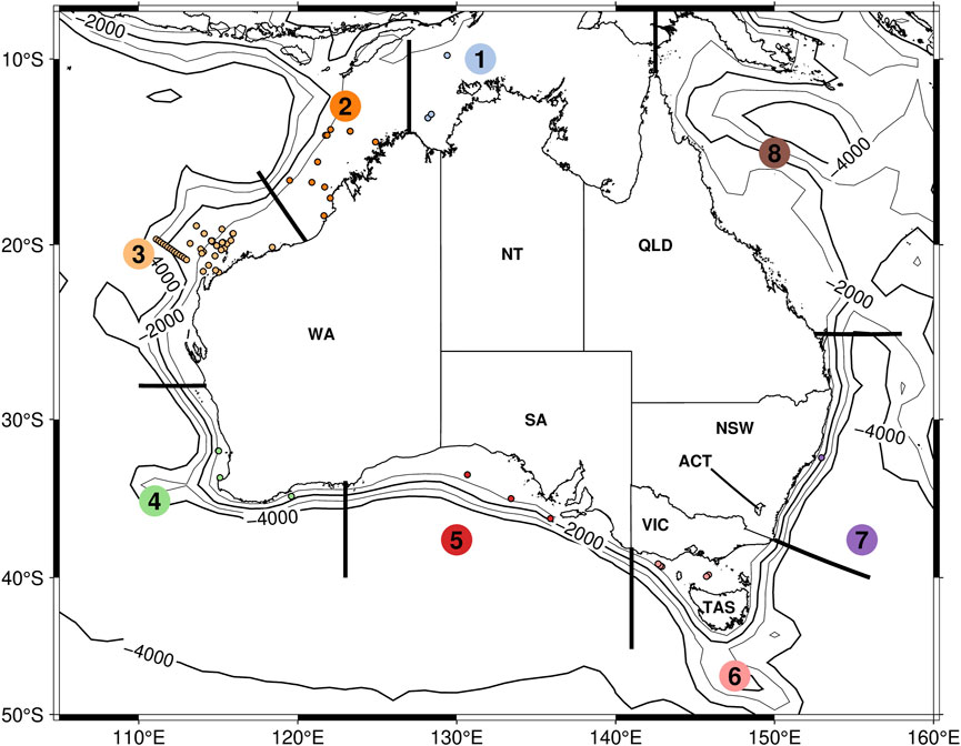
Figure 1. Locations of all acoustic datasets, grouped into marine regions. Datasets are indicated by the colored dots (each color representing one region) and the marine regions are indicated by numbers encased in colored circles.

Table 1

Table 1. Metadata for all the datasets used in the study. Bold datasets were used for the clustering experiment and the underlined datasets were used in the manual detections.

2.2 EIOPBW non-song stencils

Simultaneous visual and passive acoustic surveys had been undertaken in Geographe Bay, Western Australia, over two seasons (November of 2011 and 2012) yielding spectrogram examples of five EIOPBW non-song sound types (Recalde-Salas et al., 2014; Figure 2). The upsweep (EIO5) had been recorded only once at a medium signal-to-noise ratio and was therefore discarded. For the other sound types, spectrogram stencils were created by manually thresholding the spectrograms to values of 1 for pixels corresponding to the signal and 0 everywhere else. For the frequency-modulated call types EIO1 and 4, signal pixels were limited to the fundamental contour; for the amplitude-modulated call types EIO2 and 3, the first four harmonic contours were included. Stencils were limited to the 10–100 Hz frequency band (capturing all these calls’ main energy) and fixed at 7 s duration. The time and frequency resolutions of the stencils were 0.068 s and 1.46 Hz, respectively.

Figure 2

Figure 2. Spectrograms of EIOPBW non-song sounds recorded in Geographe Bay, Western Australia, at the time of simultaneous visual species identification. Reprinted from (Recalde-Salas et al., 2014); https://doi.org/10.1121/1.4871581; published CC BY. (a) EIO1. (b) EIO2. (c) EIO3. (d) EIO4. (e) EIO5.

2.3 Spectrogram cross-correlation

Acoustic signals matching the EIOPBW non-song stencils were found by normalized cross-correlation (Lewis, 2001). Audio recordings in our database had been sampled at various sampling rates, and so, all audio files were first resampled at 6 kHz, then converted into a spectrogram with the same time and frequency resolutions as the stencils (0.068 s and 1.46 Hz). Only the frequency band from 10 Hz to 100 Hz was searched. Each EIOPBW non-song stencil was cross-correlated with the spectrogram of the whole recording, yielding a time series of correlation coefficients (implemented using scikit-image; van der Walt et al., 2014). Correlation coefficients >0.375 were chosen to indicate a potential signal.

2.4 Manual sorting into classes

All detections output by the spectrogram-correlation detector were manually sorted into classes by two analysts (PNHD—a splitter, and CE—a lumper). The fin whale 20 Hz pulse (identified by its higher-frequency component at ∼90 Hz; Aulich et al., 2022) was detected but removed from further analysis. As classes were compared between the two analysts, the graded structure of downsweeps became obvious.

We manually identified multiple scenarios of morphing, which is the gradual transformation of a sound’s spectrographic contour in shape, frequency, and/or duration. The addition of overtones and the introduction of “embellishments” or decorations (Zwamborn and Whitehead, 2017), such as contour undulations, were also considered a morph. Several morphing examples were manually assembled both linearly (e.g., where frequency shifts higher and higher or duration extends longer and longer) and circularly (i.e., where calls morph through gradations ending at the starting point). We do not know whether the example calls were made by the same individuals or species.

The data were not pre-processed to eliminate overlapping sounds from various sources, such as vessels or other animals. The sound samples presented in the figures of this study were selected for their high signal-to-noise ratio to effectively illustrate our findings.

It is important to note that since the spectrogram cross-correlation was conducted within the 10–100 Hz frequency band, sounds above 100 Hz were not the primary targets and were detected opportunistically. This likely introduced some bias in their detections in terms of the location, season, number of occurrences, etc., as in the case of bioduck calls and some patterned sequences of downsweeps.

2.5 Manual detections

With the goal of determining the diversity of downsweeps, in addition to the five types identified by Recalde-Salas et al. (2014), a subset of recordings was manually searched (one file every 5 h from the underlined sets identified in Table 1), displaying spectrograms in Raven Pro (Cornell Lab of Ornithology, Ithaca, NY, United States). Any type of downsweep or call with downsweeping sections below 250 Hz was selected. The following frequency and time measurements were taken in Raven (see Erbe et al., 2022 for explanations).

1. Low frequency (i.e., minimum frequency of the call)

2. High frequency (i.e., maximum frequency of the call)

3. Peak frequency (i.e., frequency of peak energy)

4. Center frequency (i.e., frequency splitting the call spectrum into two-halves of equal energy)

5. 25% frequency (i.e., frequency below which 25% of the call energy lies)

6. 75% frequency (i.e., frequency below which 75% of the call energy lies)

7. 50% energy bandwidth (i.e., the difference between the 75% and 25% frequencies)

8. 90% energy bandwidth (i.e., the bandwidth centered on the center frequency and capturing 90% of the call energy)

9. Duration

10. 50% energy duration (i.e., the duration over which 50% of the energy occurs, computed as the time difference between the points in time when the 75th and 25th percentiles of cumulative energy over the full duration of the call occur)

11. 90% energy duration (i.e., the duration over which 90% of the call energy occurs)

Whether these measurements clustered was visually assessed by Principal Component Analysis (PCA) in MATLAB (The MathWorks Inc., Natick, MA, United States) using the Statistics and Machine Learning Toolbox.

2.6 Neural network detections and clustering

We further tried to get an understanding of how downsweeps would cluster using an objective neural-network approach on a subset of the datasets. The DenseNet (Miller et al., 2023), originally aimed at detecting blue whale D-calls, had been trained on a large collection of recordings from the southern seas. In addition to its geographical robustness, the trained model had also been observed to fare well in detecting generally downswept tonals that occurred within its operating bandwidth (20–115 Hz). As such, we used this model in our attempt to extract downsweeps in our EIO recordings. To keep the process tractable, we limited processing to a smaller subset comprising the datasets in bold (Table 1). To confine the outputs to only high-confidence detections, we applied a high detection threshold of 0.99. We set the clip advance amount (for converting long-duration recordings into fixed-dimension inputs to the model) to 2.0 s, resulting in 55% overlap (clip length = 4.5 s) between successive inputs to the DenseNet. While a clip overlap of more than 50% minimizes the possibility of “losing” target sounds between successive clips, it increases the possibility of a single target sound being detected in more than one clip. To suppress multiple detections of the same sound from being considered in downstream processing, we retained only the detection corresponding to the highest score within each bout of detections. This resulted in a total of 17,372 detections.

To qualitatively and visually assess potential clusters in the detected downsweeps in a 2-dimensional space, we used Uniform Manifold Approximation and Projection (UMAP; McInnes et al., 2018). We computed spectrograms of the detections (4.5 s long clips) using a 0.512 s FFT window, with 70% overlap, and frequency resolution of 1.95 Hz. By clipping frequencies outside the 20–155 Hz range, we reduced the spectrogram dimensions to 48 × 27 (height × width). Our chosen UMAP parameter settings were n_neighbors = 5, min_dist = 0.1, spread = 0.75, and repulsion_strength = 15. We arrived at these values for the parameters after intense experiments to render the 2-dimensional clustering outputs such that points in local neighborhoods were clumped closer together while the inter-cluster distances were maximized.

2.7 Geospatial and seasonal distribution

Time series of downsweep presence were plotted for each of the geospatial regions. For each recording location inside a region, the number of detections in a day was divided by the cumulative number of recording-seconds over that day and multiplied by 3,600, yielding the number of detections per hour. Then, for each day of a year for a considered region, the number of detections was averaged across all locations of the region.

2.8 Acoustic tracking of EIOPBW song and D-calls

On 9 June 2022, a sonobuoy was deployed off northwestern Australia (29°44.2014′ S, 114°13.092′ E) in Directional Frequency Analysis and Recording (DIFAR) mode, yielding bearings to acoustic sources, allowing for the direction to vocalizing animals to be calculated. Songs of EIOPBW and D-calls were recorded. Data processing steps were: 1. identifying calls in a spectrogram, 2. thresholding samples in the spectrogram by power spectral density, and 3. using the thresholded bearings to determine either mean bearing to the vocalizing animal or a distribution of bearings when there were multiple individuals vocalizing. The aim was to pinpoint D-calls to spatio-temporal tracks of singers of stereotypical (to species) songs.

3 Results

The EIOPBW non-song sound detector (spectrogram correlator) outputs nearly 129,000 calls, which were manually sorted into classes. Of these, 120,685 were downsweeps, including 6,997 of type EIO1 and 407 of type EIO4. Detections of potential EIO2 and 3 sounds were much rarer and often confounded with ship noise or EIOPBW song units, and therefore discarded from further analysis. The following sections illustrate the variability of EIO1 sounds and the gradual morphing of downsweeps.

We identified morphing cases of different downsweeps starting from the EIOPBW non-song vocalization EIO1 reported in Recalde-Salas et al. (2014). When relevant, the different sounds in the morphing plots that resembled a published spectrogram of a species were pointed out.

3.1 EIO1 morphing

EIOPBW non-song sounds of type EIO1 are ∼2–3 s long downsweeps, with the fundamental sweeping from ∼100 Hz to 30 Hz, often with harmonic overtones. Sometimes they are only weakly visible, possibly due to sound propagation effects. An example very much like that published in Recalde-Salas et al. (2014) is shown in the center (blue box) of Figure 3A. Towards the left, the sound gets shorter; towards the right, it gets longer. As indicated in the original publication (Recalde-Salas et al., 2014), EIO1 calls may begin with a little lip. The lipped variety also appears graded in duration (Figure 3B). Both lip and downsweep may change in duration—independently. The lip may start with a brief upsweep, turning it into a hat shape. The heat may become so strongly frequency-modulated (i.e., reach to rather high frequencies) that the local maximum in the contour is above the 250 Hz edge of the drawn spectrograms (Figure 3C). As already seen in Figure 3C, the lip can become more pronounced in the duration it takes up within the call, with the final concave downsweep of EIO1 shortening and disappearing altogether, at which stage, the call morphs into the entirely convex (i.e., inverted-U shaped) EIO4 (Recalde-Salas et al., 2014; Figure 3D). Finally, the EIO1 call may be emitted with various frequency-modulated “wiggly decorations”. Such alterations affect calls of all durations (shorter on the left to longer on the right of Figure 3E).

Figure 3

Figure 3. EIO1 sound morphing scenarios. All spectrograms have the same x-axis (0-7 s) and the same y-axis (10-250 Hz). (A) EIO1 sounds changing in duration from 1 s to 7 s (from panel a to panel k). The blue box in the bottom left corner shows a ∼3 s example as previously published (Recalde-Salas et al., 2014). (B) EIO1 sounds with lip at the start, changing in duration from 1 s to 7 s (from panel a to panel k). The blue box in the bottom left corner shows a ∼3 s example as previously published (Recalde-Salas et al., 2014). (C) Examples of hat shapes commonly seen at the start of EIO1 sounds. In these examples, the maximum frequency of the hat increases from panel a to panel j and is > 250 Hz in the final three plots. The blue box indicates the variant closest to the published EIO1 (Recalde-Salas et al., 2014). (D) Starting with the spectrogram in the blue box that most closely resembles an EIO1 call, the concave downsweep part shortens and disappears both to the left and to the right. The lip also becomes shorter to the left, (towards panel a) but longer to the right (towards panel k), at which stage the call has morphed into an EIO4 call (Recalde-Salas et al., 2014). (E) Wiggly versions of EIO1.

3.2 Simple downsweep morphing

The majority of downsweeps were simple downsweeps which were mostly concave (like the first half of a U) or (less often) straight. Concave downsweeps (i.e., inverted-U shape, like EIO4) were rarer. These simple downsweeps morphed in time and frequency, as did the more complex EIO1 (Figures 4A, B). Downsweeps may also gradually shift in frequency (start frequency, end frequency, and bandwidth). This variability is observed in short (<1 s) and long (>1 s) downsweeps (Figures 4C, D).

Figure 4

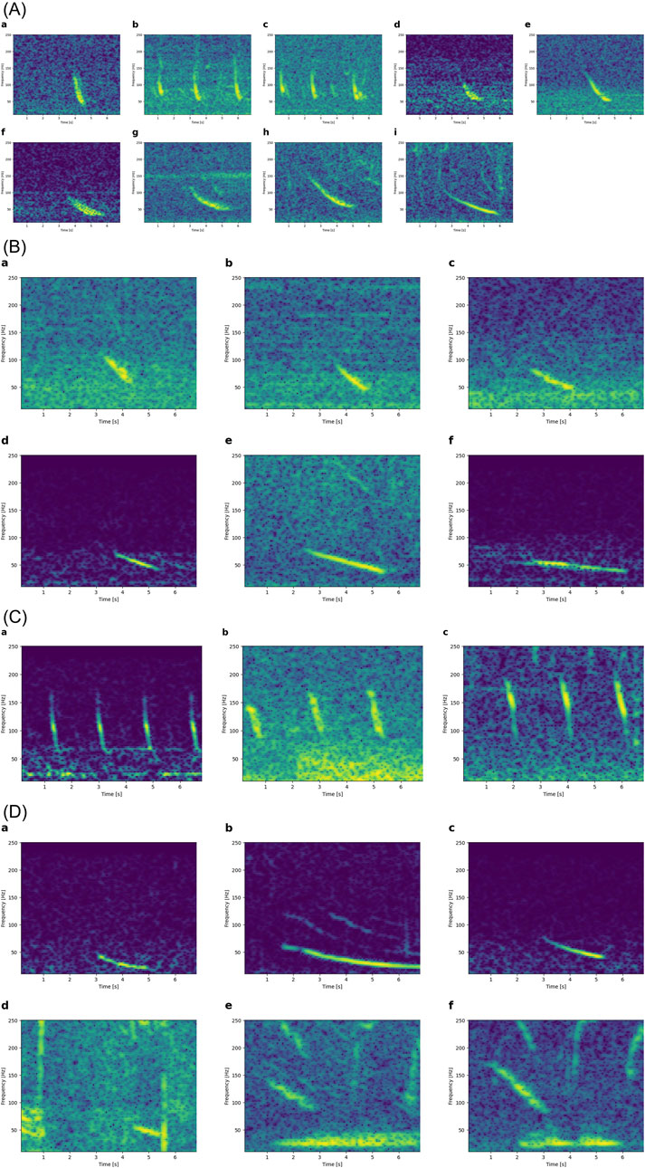
Figure 4. Simple morphing scenarios. All spectrograms have the same x-axis (0-7 s) and the same y-axis (10-250 Hz). (A) Simple concave downsweeps increasing in duration from left to right (a-i). (B) Simple straight downsweeps increasing in duration from left to right (a-f). (C) Short (<1 s) downsweeps at higher and higher frequency from left to right, without changes in duration. (D) Long (>1 s) downsweeps at increasing frequency from left to right (a-f). Note how both start and end frequency increase.

3.3 Hat-shape morphing

Downsweeps that start with an upsweep (hat shape) also grade from lower to higher frequency (Figure 5).

Figure 5

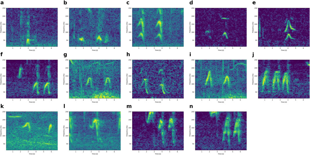
Figure 5. Illustration of hat-shaped calls gradually increasing in frequency from panel a to panel n, from a peak (maximum frequency) at ∼50 Hz (panel a) to a peak at and above 250 Hz (panel n). All spectrograms have the same axes (0-7 s and 10-250 Hz).

3.4 Wheel of downsweep contours

While the preceding sections illustrated “linear” gradations, where duration, frequency, or the number of decorations monotonically increased from image to image, the same spectrogram images were used in some of the examples, indicating that gradations occur along multiple dimensions and in multiple (back and forth) directions. We therefore also tried to arrange gradations in a circle. Many such circles are possible (Figure 6).

Figure 6

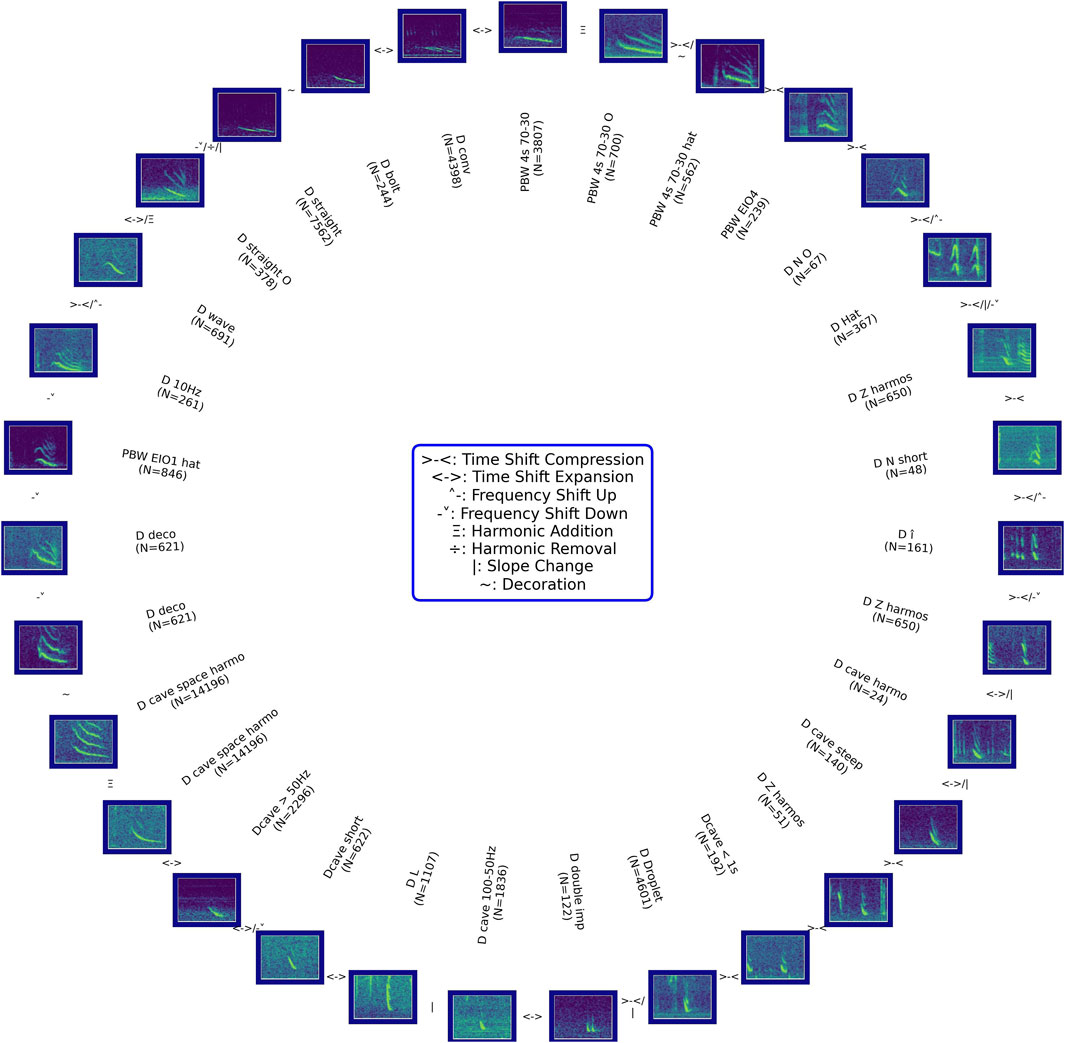
Figure 6. Wheel of gradually morphing downsweep contours. Symbols in between spectrograms indicate which feature (e.g., duration, frequency) changed and how; follow the wheel clockwise. Each spectrogram represents 7 s and the frequency ranges from 10 to 250 Hz. Each spectrogram belongs to one of the manually assigned classes (by PNHD and/or CE); N counts the number of calls in that class. Not all classes are featured. ‘PBW 4s 70–30': likely PBW downsweeps from 70 Hz to 30 Hz, 4 s; ‘PBW 4s 70O–30 O': same as ‘PBW 4s 70–30′with overtones; “PBW 4s 70–30 hat”: same as ‘PBW 4s 70O–30 O′ with a lip at the beginning; ‘PBW EIO4’: likely PBW downsweeps as described in Recalde-Salas et al., 2014; ‘D N O': downsweep with an N-shape and overtones, fundamental frequency in the band 50–100 Hz and variable duration; ‘D Hat’: hat-shape with duration <1 s and fundamental frequency within 20–100 Hz; ‘D Z harmos’: smooth Z-shape with fundamental frequency from 100 to 30 Hz, duration <2 s, with overtones, mostly identified in presence of amplitude- and frequency-modulated sounds before or after; ‘D N short’: N-shape, <1 s duration, fundamental frequency <50 Hz; ‘D î': looking similar to an I with a circumflex accent, duration <1 s and fundamental frequency >50 Hz; ‘D cave harmo’: concave shape, with overtones, fundamental frequency <50 Hz and duration <2 s; ‘D cave steep’: concave shape with steep slope and overtones, duration <2 s and fundamental frequency ranges from 100 to 30 Hz, ‘Dcave <1 s': concave shape and duration <1 s, fundamental frequency <100 Hz, ‘D Droplet’: downsweep shaped as multiple straight droplets with duration <1 s; ‘D double imp’: pygmy right whale doublet as described in Dawbin and Cato, 1992; ‘D cave 100–50 Hz’: concave between 100 and 50 Hz with variable duration between 1 s and 3 s, ‘D L': L-shape downsweep with duration <1 s, ‘Dcave short’: concave with frequency ranging from 100 to 50 Hz and duration <1 s; ‘Dcave >50Hz’: concave with frequency >50 Hz and variable durations; ‘D cave space harmo’: concave with strong harmonics, duration >2 s and fundamental frequency from 100 to below 50 Hz; ‘D deco’: downsweep with decoration, no matter its length or frequency range, ‘PBW EIO1 hat’: similar to EIO1 described in Recalde-Salas et al., 2014 with the presence of a lip at the beginning; ‘D 10Hz’: downsweep to 10 Hz regardless of its duration, bandwidth, or decorations; ‘D wave’: wave-shape downsweep with variable duration and frequency range; ‘D straight O': straight downsweep without any more complex shape, variable duration and frequency ranges from 80 to 40 Hz with overtones; ‘D straight’: same as ‘D straight O’ without overtones; ‘D bolt’: down-plateau-down shape with variable durations and frequency ranges; ‘D conv’: convex shape with different durations and frequency ranges.

3.5 Visual clustering of manual detections

Manual scrolling through spectrograms of recordings yielded 1,623 Raven selection boxes, each containing a high signal-to-noise ratio downsweep below 250 Hz. Some of these downsweeps commenced above 250 Hz. Figure 7A shows the distributions of the acoustic features. The first two principal components explained 75% of the variance in the measurements. The frequency parameters contributed strongly to the first principal component (high frequency contributed the least), while the duration and bandwidth measurements contributed strongly to the second principal component (Figure 7B). The scatter plot of Figure 7B implies that downsweeps did not separate into distinct clusters. PCA identified one potential cluster close to the center, in quadrant 2 of the component 1 versus component 2 scatter plot. The downsweeps in this cluster were all of long duration >1 s and broadband (high frequency–low frequency >100 Hz). A weaker 2^nd cluster in quadrant 3 contained short-duration (<1s) and narrowband (high frequency–low frequency <50 Hz) downsweeps. The third cluster in quadrant 4 only contained calls of high frequency (low frequency >100 Hz) and variable duration.

Figure 7

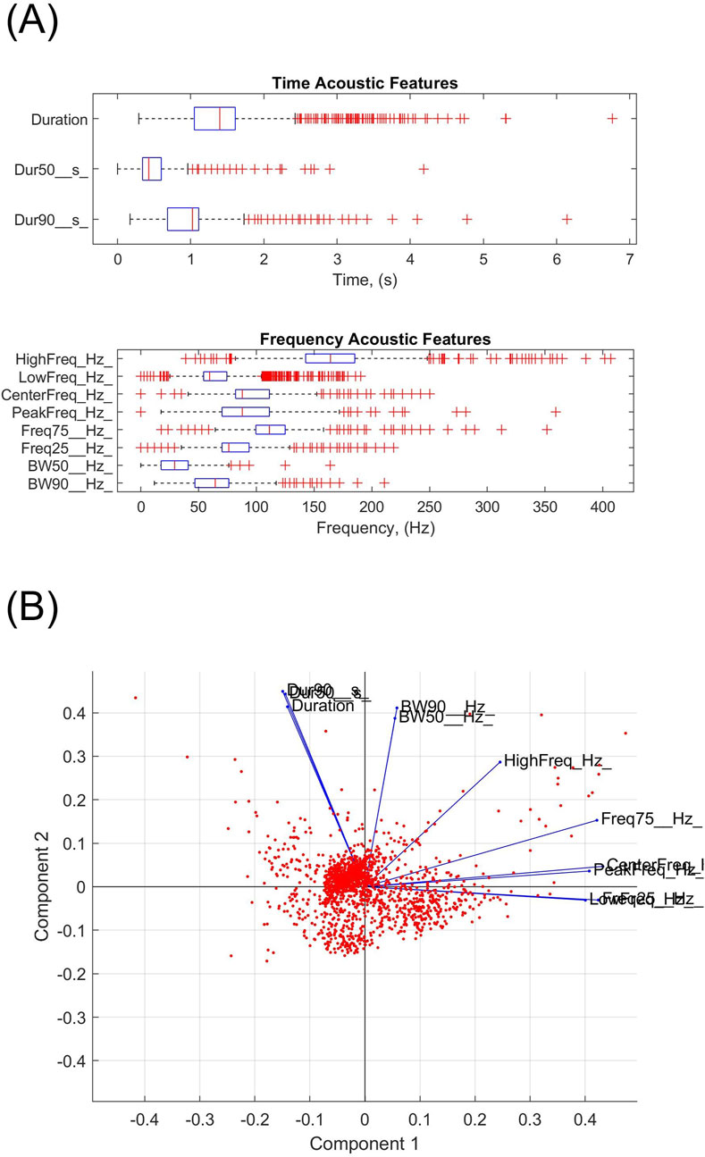
Figure 7. (A) Boxplots of the measurements of time and frequency features of 1,623 downsweeps. (B) Coefficients of the 11 parameters in their linear combinations to principal components 1 and 2. The scattered red dots correspond to the measurements of 1,623 downsweeps. The majority of calls fall into the 2nd quadrant with component 1 coefficients ranging from −0.07 to 0 and component 2 coefficients from 0 to 0.07. A weaker 2nd cluster can perhaps be identified in quadrant 3, below the x-axis and left of the y-axis. Another weak cluster exists perhaps in quadrant 4, below the x-axis and right of the y-axis.

3.6 Neural network detections and visual clustering

The 17,372 bandwidth-limited spectrograms detected with the convolutional neural network constituted the inputs to the UMAP clustering procedure. Figure 8 shows the result of the UMAP clustering process, indicating that these calls do not separate well, but rather transition smoothly.

Figure 8

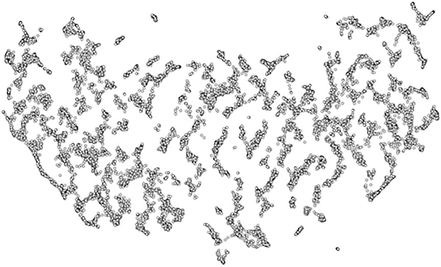
Figure 8. Clustering output from applying UMAP to the 17,372 detected downsweeps.

3.7 Co-occurrence of call types

On several occasions, the simultaneous recording of downsweeps with other call types was noted (but not systematically tracked). Examples of downsweeps in the presence of Antarctic minke whale bioducks and Omura’s whale calls are shown in Figure 9 (top and bottom row, respectively). The downsweeps did not occur at a fixed time in the other calls, and so, are not biphonations.

Figure 9

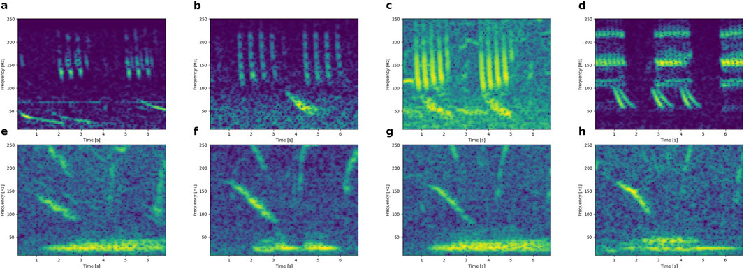
Figure 9. Downsweeps recorded together with Antarctic minke whale calls (i.e., 4-5 pulse packages >100 Hz; from panel a to panel d) and Omura’s whale calls (15–50 Hz, 5–6 s constant-wave; from panel e to panel h). X-axes: 0-7s. Y-axes: 10-250 Hz.

3.8 Patterned sequences of downsweeps

While manually sorting the 7 s spectrograms surrounding automated detections, it was noted that sometimes, downsweeps occurred in patterned sequences. These examples were kept in the hope that context around an automated detection might help identify the calling species.

The most obvious class of such sequences are the bioduck sounds from Antarctic minke whales that are packages of downsweeps, and which were present in some of our recordings (Figure 10A). Similarly, downsweep doublets were potentially from pygmy right whales, based on the spectrogram in Dawbin and Cato (1992) (Figure 10B). Additional patterned sequences are shown in Figure 10C, but no publication of these specific patterns was found. Some of these are likely humpback whales (see 1-minute-long spectrograms containing these patterns together with additional phrases; Figure 11).

Figure 10

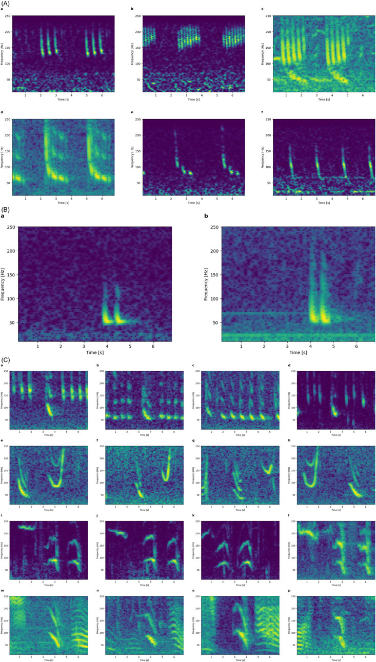
Figure 10. Patterned sequences found in the audio recordings. (A) Downsweep packages and patterns likely from Antarctic minke whales based on spectrograms published by Dominello and Sirovic. (2016). (B) Spectrograms of downsweep doublets likely from pygmy right whales based on Dawbin and Cato (1992). (C) Patterned sequences of calls involving downsweeps; each row shows four examples of the same pattern. All spectrograms are 7s long, covering 10-250 Hz.

Figure 11

Figure 11. Downsweeps as part of humpback whale song. Longer (1-minute) and more broadband (<1 kHz) examples of the patterns from Figure 10C. Note the similarities of all these harmonic 1-s downsweeps below 100 Hz to EIO1 variants (in all but the 3^rd spectrogram).

3.9 Geospatial and seasonal distribution

Maps of geospatial and seasonal distribution were drawn for all call classes. These were mostly inconclusive due to the graded nature of these calls, except for the distribution map for calls of type EIO1 (Figure 12). The West and East coast exhibited two peaks. In the Southwest and Southeast, these peaks occurred in March-May and November-December. At lower latitude, the peaks shifted to June-July and October-November, matching the known PBW migration. Only very few EIO1 detections occurred in the northernmost region (Region 1) and southernmost region (Region 5).

Figure 12

Figure 12. Annual time series of EIO1 detections by marine region. No underwater acoustic recordings were available from region 8. While there were recordings in region 7, there were no EIO1 detections.

3.10 Acoustic tracking of EIOPBW song and D-calls

Both EIOPBW songs and D-calls were recorded on the same sonobuoy for 110 min. At least two individual animals were tracked simultaneously (Figure 13). EIOPBW song was detected along both tracks; however, D-calls were only detected on one of the two tracks. These 48 D-calls were ∼3 s long, straight downsweeps from 60 Hz to 30 Hz. Morphing cases such as time stretching, a small lip at the beginning, and the addition of overtones occurred. These D-calls could be classed as a straight variant of EIO1.

Figure 13

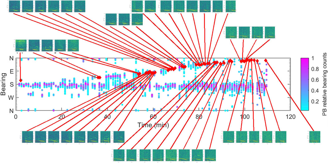
Figure 13. Bearings to EIOPBW song over time. Simultaneously recorded D-calls are indicated as red kites. Colors represent the relative number of song detections by bearing. Time resolution 1 min. All of the little spectrogram images cover 0-7s and 10-250 Hz.

4 Discussion

The main goal of this work was to build and optimize a detector for EIOPBW non-song calls, which are mostly of downsweeping type, to further study this species’ geographic and seasonal pattern of occurrence. We tried two automated detectors: 1) a simple spectrogram correlator based on stencils of confirmed (by simultaneous visual and acoustic survey; Recalde-Salas et al., 2014) EIOPBW non-song sounds, and 2) a neural network that had previously been trained on general blue whale D-calls (Miller et al., 2023) followed by an automated clustering algorithm. Upon manual checking of the auto-detections and clusters (and confirmed by manual detections, feature measurements, and PCA), we found that downsweeps exhibit great variability, do not cluster well, and instead are graded (i.e., lie along an acoustic continuum). We provided several examples of such gradations in call duration; bandwidth; start, end, and maximum frequency; presence of overtones; frequency modulations; and “decorations”.

Many other authors have noted the great variability of blue whale downsweeps in other parts of the world (e.g., Rankin et al., 2005; Berchok et al., 2006; Oleson et al., 2007a; Oleson et al., 2007b; Torterotot et al., 2023), without grading them or lining them up into a continuum. As we compared our downsweep variants to spectrograms from the literature, we noticed that along the continuum, downsweeps morph through features that have been described for other (non-blue whale) species. This raises questions about the crudeness of describing sounds from spectrographic features alone and ultimately, about our ability to generalize assignation of (non-song) sounds to species in the absence of knowledge about the ecological and behavioral contexts at the time and location of acoustic recording.

The most common call type in the observations by Recalde-Salas et al. (2014) was EIO1, also frequently observed in our datasets. This call is graded in duration, frequency, presence of overtones, and decorations. For example, the EIO1 variant in Figure 3Ad is similar to the DS1 call spectrogram published for sei whales and the EIO1 variant in Figure 3Be is similar to the DS1H call also published for sei whales (Cerchio and Weir, 2022) (Figures 14A–D). The former call type was also recorded by Tremblay et al. (2019) from sei whales, and the latter call type by Rankin and Barlow (2007) and Cusano et al. (2023) from sei whales. The EIO1 variant of Figure 3Bb resembles the humpback whale “muah” (Recalde-Salas et al., 2020) and the humpback whale B-call (D'Souza et al., 2023); variants in Figure 3Ba Ca look similar to published humpback downsweeps (call type D, Fournet et al., 2015; call type G; Epp, 2019; call type B; Saloma et al., 2022; and one call in Indeck et al., 2020). The variant in Figure 3Bc resembles the downsweep recorded from Antarctic minke whales (Casey et al., 2022). The variants with extended lips resemble calls from humpback whales (“Low Hum”, Epp, 2019; “Descending Moan” and “Wup”, (Fournet et al., 2015); “Eaw” and “Modulated call”, Cusano et al., 2020; “Screech”, (Dunlop et al., 2007), or right whales (“downcall” and “hybrid”, Webster et al., 2016), or sei whales (“arch-call”, Cerchio and Weir, 2022). Figure 3Dc, Di compare with calls from baleen whales geographically as far away as bowhead whales in the Arctic (Thode et al., 2017).

Figure 14

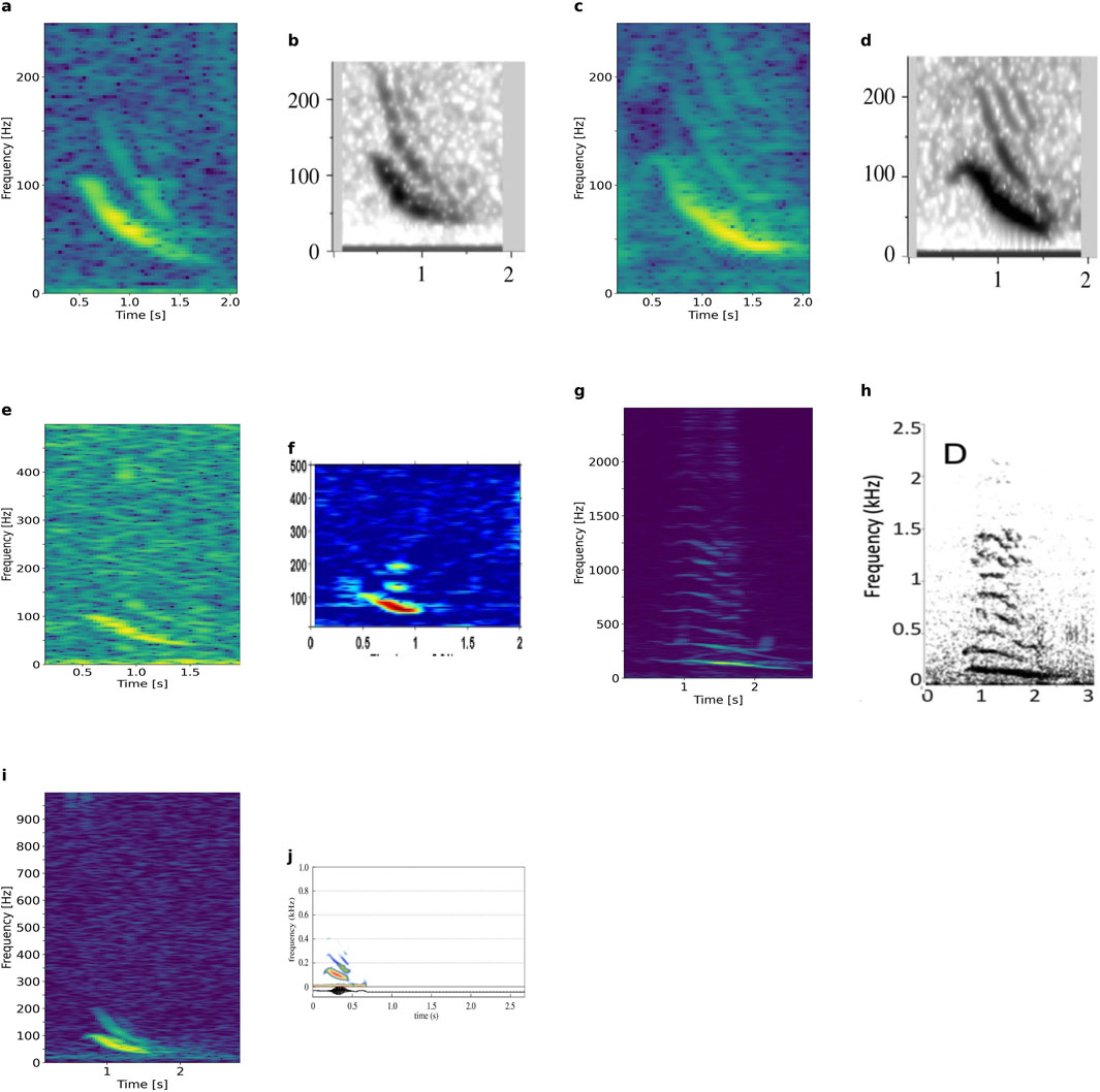
Figure 14. (a, c, e, g and i) EIO1 variants recorded in our study, which compare to similar sounds published elsewhere. (b) DS1 and (d) DS1H from sei whales (Cerchio and Weir, 2022, published CC BY 4.0). (f) Humpback whale “muah” (Recalde-Salas et al., 2020, published CC BY 4.0). (h) Humpback whale call type D (Fournet et al., 2015, reprinted with permission from the Acoustical Society of America), which is similar to call type G in Epp, 2019, call type B in Saloma et al., 2022, and one spectrogram in Indeck et al., 2020. (J) Downsweep of Antarctic minke whale (Casey et al., 2022), published CC BY 4.0.

How then can calls be assigned to species in the absence of visual validation or relevant ecological contextual knowledge? We explored 1) acoustic co-occurrence of downsweeps with species-stereotypical calls, 2) acoustic context provided by sounds before and after, and 3) geographical and seasonal occurrence of downsweeps. While downsweeps were sometimes recorded together with Antarctic minke whale bioducks (Dominello and Širović, 2016) or Omura’s whale calls (Browne et al., 2024), they occurred at variable time relative to each other and were, hence, not biphonations. With ten species of baleen whale occurring around Australia, most of which are known to migrate annually between colder (southern, in summer) and warmer (northern, in winter) grounds, co-occurrence has been noted frequently (e.g., Erbe et al., 2015), and so, sounds recorded at the same time do not have to come from the same species. Given almost all of our data were recorded with a single, omni-directional sensor, the two calling animals might not even have been at the same location. Our sonobuoy recordings provided bearing information to the calling individuals and EIO1 downsweeps followed the track of an EIOPBW singer. It is possible that the same individual produced both song and downsweeps, or that a singer and non-song producer traveled closely together in a small cohort. In the latter case, given the two sound types were tracked together for 80 min, it is likely that the cohort consisted of individuals of the same species and therefore, that those downsweeps were indeed made by an EIOPBW.

Acoustic context can be derived from other sounds occurring before or after a downsweep. Some of our downsweep detections were part of patterned sequences or songs. Humpback whales produce complex songs, using a great variety of units in long and hierarchical patterns (Payne and McVay, 1971) and some of our downsweeps were part of these complex patterns, but not all. For downsweeps in simpler or no patterns, identification to species was thus inconclusive.

Ecological and behavioral context in a given region can also inform species identification. For instance, seasonally occurring downsweeps during known migratory periods of PBW may be attributable to the species with a high level of certainty in locations where other species that produce downsweeps are very unlikely to occur. The geographic and seasonal occurrence of downsweeps resembling EIO1 from Recalde-Salas et al. (2014) reported here is an example where knowledge of the migratory timing of PBWs corroborates downsweep attribution to the species. For downsweeps not resembling EIO1, looking at the geographic and seasonal occurrence, however, was inconclusive as they could not be separated into clusters.

More work needs to be done before downsweeps as single spectrographic features, in the absence of regional ecological and behavioral context, can perhaps be used routinely in environmental mitigation and monitoring plans. First, beginning with automated detectors, there will always be a trade-off between precision and recall, between false alarms and missed detections. More specifically, spectrogram correlation detectors are known to suffer from a lack of variability in the detected signals due to fixed templates (Socheleau et al., 2015). Their advantages are that they are intuitive, simple, and quick to set up; they do not require the creation of a training database for dictionary-based methods or neural networks. Second, sorting detections into classes is prone to biases. The UMAP algorithm was unable to cluster downsweeps—partly because downsweeps are graded. Moreover, similar call types were found in different clusters because of different ambient noise in the recordings. Even for high signal-to-noise ratio examples, UMAP may cluster based on noise features as the algorithm is influenced by both local and global structures in the data (McInnes et al., 2018). Statistical clustering techniques could have been applied to quantify the lack of clusters in the data. However, these methods also suffer from drawbacks such as sensitivity to noise, dependence on predefined parameters, and the potential to detect spurious clusters that do not reflect meaningful differences in the data. Furthermore, clustering algorithms may impose artificial groupings based on mathematical assumptions rather than perceptual or biologically relevant differences in the sounds. Therefore, given that neither PCA or UMAP revealed clusters, a visual inspection was considered sufficient to conclude that the calls do not naturally cluster. Finally, manual sorting of detections, apart from being overwhelming, is biased by human perception (Leroy et al., 2018; Nguyen Hong Duc et al., 2021; Dubus et al., 2024). One solution to averaging out the bias in the human error could be to have citizen scientists annotate the data (Nguyen Hong Duc et al., 2021; Dubus et al., 2024). This solution has limitations, however, because the results may be prone to greater error and lower precision, and the bias will still be present due to, for example, how the citizen scientists were trained, their previous experience in annotating, and the material they use for training. Additional improvements, in particular for highly variable calls like downsweeps, might be achieved by soft instead of hard labels for sounds, such as probabilities for belonging to a type, population, or species, rather than discrete call categories.

Given the similarities of call types across different species, we might need to improve our ways of measuring and describing these sounds. Transforms other than the Fourier transform (e.g., wavelet transforms; Urazghildiiev and Clark, 2007; Mouy et al., 2008) might capture different features and separate calls differently. Correcting for the effects of the sound propagation environment could help (e.g., removing echoes, frequency-dependent absorption, and dispersion; Erbe et al., 2022), but the location of the calling animal is typically unknown in recordings from single, autonomous deployments. Furthermore, a common library of audio sounds (Miller et al., 2021; Parsons et al., 2024) with associated metadata (site, time of the year, sampling frequency, supposed category) could enable researchers to compare their annotations and increase their training, testing, and reference database.

Finally, tools derived from phonetic science might improve researchers’ accuracy in identifying species producing specific call types. Phonetic science focuses on a combination of physical properties, perception, and transmission of sounds and language (Kortmann, 2020), in the context of recognizing, categorizing, and understanding sounds. Species could have differences in pitch and loudness that could contribute to manual downsweep identification; albeit for sounds having frequencies below those humans are sensitive to, these would need to be sped up during playback. Although perception of sounds is inherently biased, theories and tools on speech perception and sound production in humans may help manual categorization of sounds accounting for how these are processed by the brain. Until further advances can be made to allow full automation of downsweep detection as single spectrographic features, the extent of interpretation of results and their attribution to species will need to be informed by regional ecological and behavioral knowledge and manual reviewing of acoustic data by experienced personnel in the identification of sounds spectrographically and phonetically. Then, an integrated approach drawing from different disciplines could be a critical pathway to progress automated classification of downsweeps at the species level.

In conclusion, we showed that downsweeps do not cluster; instead, they are graded and morph along a continuum of acoustic features. We also demonstrated the challenges in classifying downsweeps to species, with similar downsweep types having been reported from diverse species of mysticete whales. Hence, not all low-frequency downsweeps (<100 Hz) are blue whales. Even humpback whales have downsweeps to below 50 Hz in their songs. While automated passive acoustic monitoring for environmental management would ideally detect non-song sounds in addition to species-stereotypical song (in order to not only increase the probability of detection but also monitor the non-singing demographics), reliance on downsweeps alone is marred with several challenges—at this stage.

Data availability statement

Some of the raw recordings are available from the Australian Ocean Data Network; Passive Acoustic Observatories Sub-Facility by Curtin University; https://portal.aodn.org.au/. The spectrogram images used in this study are available to any interested party upon request to the corresponding author.

Ethics statement

Ethical approval was not required in accordance with the local legislation and institutional requirements because the majority of data (underwater acoustic recordings) were collected for a quantification of ambient ocean noise rather than research on animals. Animal ethics for remote passive acoustic monitoring was not required for the collection of the early datasets. The recent acoustic datasets were collected under Curtin University Animal Ethics approvals AEC-2013–28 and ARE-2021–11.

Author contributions

PNHD: Conceptualization, Data curation, Formal Analysis, Investigation, Methodology, Software, Supervision, Validation, Visualization, Writing–original draft, Writing–review and editing. CE: Conceptualization, Data curation, Formal Analysis, Funding acquisition, Methodology, Project administration, Supervision, Validation, Writing–review and editing. SM: Validation, Visualization, Writing–review and editing, Investigation, Methodology, Software. DW: Data curation, Investigation, Software, Writing–review and editing. LG: Data curation, Methodology, Software, Visualization, Writing–review and editing. CT: Data curation, Methodology, Software, Visualization, Writing–review and editing. ND: Data curation, Writing–review and editing. AE: Data curation, Writing–review and editing. CJ: Resources, Writing–review and editing. MJ: Resources, Writing–review and editing. AR-S: Resources, Writing–review and editing. CS: Resources, Writing–review and editing. KS: Data curation, Writing–review and editing. CW: Data curation, Writing–review and editing. RM: Funding acquisition, Resources, Writing–review and editing.

Funding

The author(s) declare that financial support was received for the research and/or publication of this article. Partial support by Chevron Australia.

Acknowledgments

We thank Chevron Australia, Woodside Energy Ltd as Operator for and on behalf of the Browse Joint Venture (BJV), Fugro, BHP, INPEX, and the SeaWorld and Busch Gardens Conservation Fund for supporting some of the data collection and analyses. Additional datasets were provided by Geoscience Australia and had been collected with ocean bottom seismographs by the ANSIR Research Facilities for Earth Sounding. Some datasets were sourced from Australia’s Integrated Marine Observing System (IMOS) enabled by the National Collaborative Research Infrastructure Strategy (NCRIS). IMOS is operated by a consortium of institutions as an unincorporated joint venture, with the University of Tasmania as Lead Agent.

Conflict of interest

Authors CJ and MJ were employed by Centre for Whale Research (WA) Inc.

The remaining authors declare that the research was conducted in the absence of any commercial or financial relationships that could be construed as a potential conflict of interest.

Generative AI statement

The author(s) declare that no Generative AI was used in the creation of this manuscript.

Publisher’s note

All claims expressed in this article are solely those of the authors and do not necessarily represent those of their affiliated organizations, or those of the publisher, the editors and the reviewers. Any product that may be evaluated in this article, or claim that may be made by its manufacturer, is not guaranteed or endorsed by the publisher.

Footnotes

¹Australian Government, Geoscience Australia, “Offshore Northwest Australia”; https://www.ga.gov.au/scientific-topics/energy/province-sedimentary-basin-geology/petroleum/offshore-northwest-australia; last updated 29 August 2023.

²Australian Government, Department of Climate Change, Energy, the Environment and Water, “Indian Ocean off the Bunbury region, Western Australia declared offshore wind area; https://www.dcceew.gov.au/energy/renewable/offshore-wind/areas/bunbury; accessed 13 October 2024.

³Government of Western Australia, Westport, “A new port in Kwinana: Planning for the next century of trade growth in WA”; https://westport.wa.gov.au/; accessed 13 October 2024.

⁴Gascoyne Gateway; https://gascoynegateway.com.au/; accessed 13 October 2024.

⁵Australian Government, Department of Climate Change, Energy, the Environment and Water, “EPBC Act List of Threatened Fauna”; https://www.environment.gov.au/cgi-bin/sprat/public/publicthreatenedlist.pl?wanted=fauna#mammals_endangered; accessed 13 October 2024.

⁶CHORUS software; https://cmst.curtin.edu.au/products/chorus-software/; accessed 13 October 2024.

⁷Australian Government, “Australia’s marine regions”; https://www.waterquality.gov.au/anz-guidelines/your-location/australia-marine-regions; accessed 15 October 2024.

References

Aulich, M. G., McCauley, R. D., Miller, B. S., Samaran, F., Giorli, G., Saunders, B. J., et al. (2022). Seasonal distribution of the fin whale (Balaenoptera physalus) in Antarctic and Australian waters based on passive acoustics. Front. Mar. Sci. 9, 864153. doi:10.3389/fmars.2022.864153

CrossRef Full Text | Google Scholar

Australian Government (2013). “Marine Nation 2025: marine science to support Australia’s blue economy,” in Oceans policy science advisory group (Canberra, Australia).

Google Scholar

Australian Government (2015). Conservation management Plan for the blue whale 2015-2025. Canberra, ACT, Australia: department of climate change. Energy. the Environment and Water.

Google Scholar

Berchok, C. L., Bradley, D. L., and Gabrielson, T. B. (2006). St. Lawrence blue whale vocalizations revisited: characterization of calls detected from 1998 to 2001. J. Acoust. Soc. Am. 120 (4), 2340–2354. doi:10.1121/1.2335676

PubMed Abstract | CrossRef Full Text | Google Scholar

Browne, C. E., Erbe, C., and McCauley, R. D. (2024). Distribution and seasonality of the Omura’s whale (Balaenoptera omurai) in Australia based on passive acoustic recordings. Animals 14 (20), 2944. doi:10.3390/ani14202944

PubMed Abstract | CrossRef Full Text | Google Scholar

Casey, C. B., Weindorf, S., Levy, E., Linsky, J. M. J., Cade, D. E., Goldbogen, J. A., et al. (2022). Acoustic signalling and behaviour of Antarctic minke whales (Balaenoptera bonaerensis). R. Soc. Open Sci. 9 (7), 211557. doi:10.1098/rsos.211557

PubMed Abstract | CrossRef Full Text | Google Scholar

Cerchio, S., and Weir, C. R. (2022). Mid-frequency song and low-frequency calls of sei whales in the Falkland Islands. R. Soc. Open Sci. 9 (11), 220738. doi:10.1098/rsos.220738

PubMed Abstract | CrossRef Full Text | Google Scholar

Cusano, D. A., Indeck, K. L., Noad, M. J., and Dunlop, R. A. (2020). Humpback whale (Megaptera novaeangliae) social call production reflects both motivational state and arousal. Bioacoustics 31, 17–40. doi:10.1080/09524622.2020.1858450

CrossRef Full Text | Google Scholar

Cusano, D. A., Indeck, K. L., Noad, M. J., and Dunlop, R. A. (2022). Humpback whale (Megaptera novaeangliae) social call production reflects both motivational state and arousal. Bioacoustics 31 (1), 17–40. doi:10.1080/09524622.2020.1858450

CrossRef Full Text | Google Scholar

Cusano, D. A., Wiley, D., Zeh, J. M., Kerr, I., Pensarosa, A., Zadra, C., et al. (2023). Acoustic recording tags provide insight into the springtime acoustic behavior of sei whales in Massachusetts Bay. J. Acoust. Soc. Am. 154 (6), 3543–3555. doi:10.1121/10.0022570

PubMed Abstract | CrossRef Full Text | Google Scholar

Dawbin, W. H., and Cato, D. H. (1992). Sounds of a pygmy right whale (Caperea marginata). Mar. Mammal Sci. 8 (3), 213–219. doi:10.1111/j.1748-7692.1992.tb00405.x

CrossRef Full Text | Google Scholar

Dominello, T., and Širović, A. (2016). Seasonality of Antarctic minke whale (Balaenoptera bonaerensis) calls off the western Antarctic Peninsula. Mar. Mammal Sci. 32 (3), 826–838. doi:10.1111/mms.12302

CrossRef Full Text | Google Scholar

D'Souza, M. L., Bopardikar, I., Sutaria, D., and Klinck, H. (2023). Arabian Sea humpback whale (Megaptera novaeangliae) singing activity off Netrani Island, India. Aquat. Mamm. 49 (3), 223–235. doi:10.1578/AM.49.3.2023.223

CrossRef Full Text | Google Scholar

Dubus, G., Cazau, D., Torterotot, M., Gros-Martial, A., Nguyen Hong Duc, P., and Adam, O. (2024). From citizen science to AI models: advancing cetacean vocalization automatic detection through multi-annotator campaigns. Ecol. Inf. 81, 102642. doi:10.1016/j.ecoinf.2024.102642

CrossRef Full Text | Google Scholar

Dunlop, R. A., Noad, M. J., Cato, D. H., and Stokes, D. (2007). The social vocalization repertoire of east Australian migrating humpback whales (Megaptera novaeangliae). J. Acoust. Soc. Am. 122 (5), 2893–2905. doi:10.1121/1.2783115

PubMed Abstract | CrossRef Full Text | Google Scholar

Epp, M. (2019). The call repertoire of humpback whales (Megaptera novaeangliae) on a Newfoundland foraging ground (2015, 2016) with comparison to a Hawaiian breeding ground (1981, 1982) (Canada: University of Manitoba). M.Sc. Thesis.

Google Scholar

Erbe, C., Duncan, A., and Vigness-Raposa, K. J. (2022). “Introduction to sound propagation under water,” in Exploring animal behavior through sound Methods. Editors C. Erbe, and J. A. Thomas (Cham: Springer International Publishing), Vol. 1, 185–216. doi:10.1007/978-3-030-97540-1_6

CrossRef Full Text | Google Scholar

Erbe, C., Verma, A., McCauley, R., Gavrilov, A., and Parnum, I. (2015). The marine soundscape of the Perth Canyon. Prog. Oceanogr. 137, 38–51. doi:10.1016/j.pocean.2015.05.015

CrossRef Full Text | Google Scholar

Fournet, M. E., Szabo, A., and Mellinger, D. K. (2015). Repertoire and classification of non-song calls in Southeast Alaskan humpback whales (Megaptera novaeangliae). J. Acoust. Soc. Am. 137 (1), 1–10. doi:10.1121/1.4904504

PubMed Abstract | CrossRef Full Text | Google Scholar

Gavrilov, A., McCauley, R., and Gedamke, J. (2012). Steady inter and intra-annual decrease in the vocalization frequency of Antarctic blue whales. J. Acoust. Soc. Am. 131 (6), 4476–4480. doi:10.1121/1.4707425

PubMed Abstract | CrossRef Full Text | Google Scholar

Gavrilov, A., McCauley, R., Salgado-Kent, C., Tripovich, J., and Burton, C. (2011). Vocal characteristics of pygmy blue whales and their change over time. J. Acoust. Soc. Am. 130 (6), 3651–3660. doi:10.1121/1.3651817

PubMed Abstract | CrossRef Full Text | Google Scholar

Gavrilov, A. N., and McCauley, R. D. (2013). Acoustic detection and long-term monitoring of pygmy blue whales over the continental slope in southwest Australia. J. Acoust. Soc. Am. 134 (3), 2505–2513. doi:10.1121/1.4816576

PubMed Abstract | CrossRef Full Text | Google Scholar

Gavrilov, A. N., and Parsons, M. J. G. (2014). A Matlab tool for the characterisation of recorded underwater sound (CHORUS). Acoust. Aust. 42 (3), 190–196.

Google Scholar

Guilment, T., Socheleau, F.-X., Pastor, D., and Vallez, S. (2018). Sparse representation-based classification of mysticete calls. J. Acoust. Soc. Am. 144 (3), 1550–1563. doi:10.1121/1.5055209

PubMed Abstract | CrossRef Full Text | Google Scholar

Huang, G., Liu, Z., Maaten, L. V. D., and Weinberger, K. Q. (2017). “Densely connected convolutional networks,” in Paper presented at the 2017 IEEE Conference on Computer Vision and Pattern Recognition (CVPR), USA, July 26 2017. doi:10.1109/CVPR.2017.243

CrossRef Full Text | Google Scholar

Indeck, K. L., Girola, E., Torterotot, M., Noad, M. J., and Dunlop, R. A. (2020). Adult female-calf acoustic communication signals in migrating east Australian humpback whales. Bioacoustics 30 (3), 341–365. doi:10.1080/09524622.2020.1742204

CrossRef Full Text | Google Scholar

Jolliffe, C. D., McCauley, R. D., and Gavrilov, A. N. (2023). Variability in temporal characteristics of the South Eastern Indian Ocean pygmy blue whale song. Animal Behav. Cognition 10 (3), 211–231. doi:10.26451/abc.10.03.02.2023

CrossRef Full Text | Google Scholar

Kortmann, B. (2020). Phonetics and phonology: on sounds and sound systems. Stuttg. J.B. Metzler, 27–50. doi:10.1007/978-3-476-05678-8_2

CrossRef Full Text | Google Scholar

Leroy, E. C., Royer, J.-Y., Alling, A., Maslen, B., and Rogers, T. L. (2021). Multiple pygmy blue whale acoustic populations in the Indian Ocean: whale song identifies a possible new population. Sci. Rep. 11 (1), 8762. doi:10.1038/s41598-021-88062-5

PubMed Abstract | CrossRef Full Text | Google Scholar

Leroy, E. C., Thomisch, K., Royer, J.-Y., Boebel, O., and Van Opzeeland, I. (2018). On the reliability of acoustic annotations and automatic detections of Antarctic blue whale calls under different acoustic conditions. J. Acoust. Soc. Am. 144 (2), 740–754. doi:10.1121/1.5049803

PubMed Abstract | CrossRef Full Text | Google Scholar

Lewis, J. P. (2001). Fast normalized cross-correlation. Industrial Light and Magic 10, 7.

Google Scholar

Lewis, L. A., Calambokidis, J., Stimpert, A. K., Fahlbusch, J., Friedlaender, A. S., McKenna, M. F., et al. (2018). Context-dependent variability in blue whale acoustic behaviour. R. Soc. Open Sci. 5 (8), 180241. doi:10.1098/rsos.180241

PubMed Abstract | CrossRef Full Text | Google Scholar

McDonald, M. A., Calambokidis, J., Teranishi, A. M., and Hildebrand, J. A. (2001). The acoustic calls of blue whales off California with gender data. J. Acoust. Soc. Am. 109 (4), 1728–1735. doi:10.1121/1.1353593

PubMed Abstract | CrossRef Full Text | Google Scholar

McInnes, L., Healy, J., Saul, N., and Großberger, L. (2018). UMAP: Uniform Manifold approximation and projection. J. Open Source Softw. 3 (29), 861. doi:10.21105/joss.00861

CrossRef Full Text | Google Scholar

Miller, B. S., Collins, K., Barlow, J., Calderan, S., Leaper, R., Mark, M., et al. (2014). Blue whale vocalizations recorded around New Zealand: 1964-2013. J. Acoust. Soc. Am. 135 (3), 1616–1623. doi:10.1121/1.4863647

PubMed Abstract | CrossRef Full Text | Google Scholar

Miller, B. S., Madhusudhana, S., Aulich, M. G., and Kelly, N. (2023). Deep learning algorithm outperforms experienced human observer at detection of blue whale D-calls: a double-observer analysis. Remote Sens. Ecol. Conservation 9 (1), 104–116. doi:10.1002/rse2.297

CrossRef Full Text | Google Scholar

Miller, B. S., The, I.-S. S. A. T. W. G., Kathleen, M., Balcazar, N., Nieukirk, S., Leroy, E. C., et al. (2021). An open access dataset for developing automated detectors of Antarctic baleen whale sounds and performance evaluation of two commonly used detectors. Sci. Rep. 11 (1), 806. doi:10.1038/s41598-020-78995-8

PubMed Abstract | CrossRef Full Text | Google Scholar

Mouy, X., Leary, D., Martin, B., and Laurinolli, M. (2008). A comparison of methods for the automatic classification of marine mammal vocalizations in the Arctic. Passive '08 2008 New Trends Environ. Monit. Using Passive Syst., 67–72. doi:10.1109/PASSIVE.2008.4786984

CrossRef Full Text | Google Scholar

Nguyen Hong Duc, P., Torterotot, M., Samaran, F., White, P. R., Gérard, O., Adam, O., et al. (2021). Assessing inter-annotator agreement from collaborative annotation campaign in marine bioacoustics. Ecol. Inf. 61, 101185. doi:10.1016/j.ecoinf.2020.101185

CrossRef Full Text | Google Scholar

Oleson, E. M., Calambokidis, J., Burgess, W. C., McDonald, M. A., LeDuc, C. A., and Hildebrand, J. A. (2007a). Behavioral context of call production by eastern North Pacific blue whales. Mar. Ecol. Prog. Ser. 330, 269–284. doi:10.3354/meps330269

CrossRef Full Text | Google Scholar

Oleson, E. M., Wiggins, S. M., and Hildebrand, J. A. (2007b). Temporal separation of blue whale call types on a southern California feeding ground. Anim. Behav. 74 (4), 881–894. doi:10.1016/j.anbehav.2007.01.022

CrossRef Full Text | Google Scholar

Parsons, M. J. G., Looby, A., Chanda, K., Di Iorio, L., Erbe, C., Frazao, F., et al. (2024). “A global library of underwater biological sounds (GLUBS): an online platform with multiple passive acoustic monitoring applications,” in The effects of noise on aquatic life: principles and practical considerations. Editors A. N. Popper, J. A. Sisneros, A. D. Hawkins, and F. Thomsen (Cham: Springer International Publishing), 2149–2173. doi:10.1007/978-3-031-50256-9_123

CrossRef Full Text | Google Scholar

Payne, R. S., and McVay, S. (1971). Songs of humpback whales. Science 173 (3997), 585–597. doi:10.1126/science.173.3997.585

PubMed Abstract | CrossRef Full Text | Google Scholar

Rankin, S., and Barlow, J. (2007). Vocalizations of the sei whale Balaenoptera borealis off the Hawaiian Islands. Bioacoustics 16 (2), 137–145. doi:10.1080/09524622.2007.9753572

CrossRef Full Text | Google Scholar

Rankin, S., Ljungblad, D., Clark, C. W., and Kato, H. (2005). Vocalisations of Antarctic blue whales, Balaenoptera musculus intermedia, recorded during the 2001/2002 and 2002/2003 IWC/SOWER circumpolar cruises, Area V, Antarctica. J. Cetacean Res. Manag. 7 (1), 13–20. doi:10.47536/jcrm.v7i1.752

CrossRef Full Text | Google Scholar

Rasmussen, J. H., and Širović, A. (2021). Automatic detection and classification of baleen whale social calls using convolutional neural networks. J. Acoust. Soc. Am. 149 (5), 3635–3644. doi:10.1121/10.0005047

PubMed Abstract | CrossRef Full Text | Google Scholar

Recalde-Salas, A., Erbe, C., Salgado Kent, C., and Parsons, M. (2020). Non-song vocalizations of humpback whales in Western Australia. Front. Mar. Sci. 7 (141). doi:10.3389/fmars.2020.00141

CrossRef Full Text | Google Scholar

Recalde-Salas, A., Salgado Kent, C. P., Parsons, M. J. G., Marley, S. A., and McCauley, R. D. (2014). Non-song vocalizations of pygmy blue whales in Geographe Bay, Western Australia. J. Acoust. Soc. Am. 135 (5), EL213–EL218. doi:10.1121/1.4871581

PubMed Abstract | CrossRef Full Text | Google Scholar

Saloma, A., Ratsimbazafindranahaka, M. N., Martin, M., Andrianarimisa, A., Huetz, C., Olivier, A., et al. (2022). Social calls in humpback whale mother-calf groups off Sainte Marie breeding ground (Madagascar, Indian Ocean). PeerJ 10, e13785. doi:10.7717/peerj.13785

PubMed Abstract | CrossRef Full Text | Google Scholar

Schall, E., Di Iorio, L., Berchok, C., Filún, D., Bedriñana-Romano, L., Buchan, S. J., et al. (2020). Visual and passive acoustic observations of blue whale trios from two distinct populations. Mar. Mammal Sci. 36 (1), 365–374. doi:10.1111/mms.12643

CrossRef Full Text | Google Scholar

Socheleau, F.-X., Leroy, E., Pecci, A. C., Samaran, F., Bonnel, J., and Royer, J.-Y. (2015). Automated detection of Antarctic blue whale calls. J. Acoust. Soc. Am. 138 (5), 3105–3117. doi:10.1121/1.4934271

PubMed Abstract | CrossRef Full Text | Google Scholar

Thode, A. M., Blackwell, S. B., Conrad, A. S., Kim, K. H., and Macrander, A. M. (2017). Decadal-scale frequency shift of migrating bowhead whale calls in the shallow Beaufort Sea. J. Acoust. Soc. Am. 142 (3), 1482–1502. doi:10.1121/1.5001064

PubMed Abstract | CrossRef Full Text | Google Scholar

Torterotot, M., Royer, J. Y., and Samaran, F. (2019). “Detection strategy for long-term acoustic monitoring of blue whale stereotyped and non-stereotyped calls in the Southern Indian Ocean,” in Paper presented at the OCEANS 2019. Marseille. doi:10.1109/OCEANSE.2019.8867271

CrossRef Full Text | Google Scholar

Torterotot, M., Samaran, F., and Royer, J.-Y. (2023). Long-term acoustic monitoring of nonstereotyped blue whale calls in the southern Indian Ocean. Mar. Mammal Sci. 39 (2), 594–610. doi:10.1111/mms.12998

CrossRef Full Text | Google Scholar

Tremblay, C. J., Parijs, S. M. V., and Cholewiak, D. (2019). 50 to 30-Hz triplet and singlet down sweep vocalizations produced by sei whales (Balaenoptera borealis) in the western North Atlantic Ocean. J. Acoust. Soc. Am. 145 (6), 3351–3358. doi:10.1121/1.5110713

PubMed Abstract | CrossRef Full Text | Google Scholar

Urazghildiiev, I. R., and Clark, C. W. (2007). Acoustic detection of North Atlantic right whale contact calls using spectrogram-based statistics. J. Acoust. Soc. Am. 122 (2), 769–776. doi:10.1121/1.2747201

PubMed Abstract | CrossRef Full Text | Google Scholar

van der Walt, S., Schönberger, J. L., Nunez-Iglesias, J., Boulogne, F., Warner, J. D., Yager, N., et al. (2014). scikit-image: image processing in Python. PeerJ 2, e453. doi:10.7717/peerj.453

PubMed Abstract | CrossRef Full Text | Google Scholar

Verfuss, U. K., Gillespie, D., Gordon, J., Marques, T. A., Miller, B., Plunkett, R., et al. (2018). Comparing methods suitable for monitoring marine mammals in low visibility conditions during seismic surveys. Mar. Pollut. Bull. 126, 1–18. doi:10.1016/j.marpolbul.2017.10.034

PubMed Abstract | CrossRef Full Text | Google Scholar

Webster, T. A., Dawson, S. M., Rayment, W. J., Parks, S. E., and Van Parijs, S. M. (2016). Quantitative analysis of the acoustic repertoire of southern right whales in New Zealand. J. Acoust. Soc. Am. 140 (1), 322–333. doi:10.1121/1.4955066

PubMed Abstract | CrossRef Full Text | Google Scholar

Zwamborn, E. M. J., and Whitehead, H. (2017). The baroque potheads: modification and embellishment in repeated call sequences of long-finned pilot whales. Behaviour 154 (9-10), 963–979. doi:10.1163/1568539X-00003451

CrossRef Full Text | Google Scholar