BERT Bi-modal self-supervised learning for crop classification using Sentinel-2 and Planetscope

Crop identification and monitoring of crop dynamics are essential for agricultural planning, environmental monitoring, and ensuring food security. Recent advancements in remote sensing technology and state-of-the-art machine learning have enabled large-scale automated crop classification. However, these methods rely on labeled training data, which requires skilled human annotators or extensive field campaigns, making the process expensive and time-consuming. Self-supervised learning techniques have demonstrated promising results in leveraging large unlabeled datasets across domains. Yet, self-supervised representation learning for crop classification from remote sensing time series remains under-explored due to challenges in curating suitable pretext tasks. While bimodal self-supervised approaches combining data from Sentinel-2 and Planetscope sensors have facilitated pre-training, existing methods primarily exploit the distinct spectral properties of these complementary data sources. In this work, we propose novel self-supervised pre-training strategies inspired from BERT that leverage both the spectral and temporal resolution of Sentinel-2 and Planetscope imagery. We carry out extensive experiments comparing our approach to existing baseline setups across nine test cases, in which our method outperforms the baselines in eight instances. This pre-training thus offers an effective representation of crops for tasks such as crop classification.

1 Introduction

Crop classification is the process of identifying crops at a particular location based on the temporal pattern of their spectral signature obtained from satellite missions. The evolution of the spectral signature, which varies from crop to crop, is influenced by the crop’s phenological traits such as its life cycle stages (seeding, budding, growing, and sprouting) (Meier et al., 2009). Thus, temporal information plays a crucial role in crop classification by capturing these phenological patterns over the growing season. Exploiting the temporal information will help in various applications such as optimizing farming practices and increasing crop yields.

Accurate crop classification from satellite imagery is crucial for agricultural monitoring (Luo et al., 2024), yield estimation (Dell’Acqua et al., 2018), and ensuring food security (Ray et al., 2022). Satellite missions such as Sentinel-2 (Drusch et al., 2012) have provided large amounts of data, but annotating them is costly and laborious. Conventional approaches like random forest algorithms have shown limitations in their ability to generalize effectively. These models struggle to accurately predict outcomes for crop fields at different locations and even the same crop fields at different time points, as evidenced by (Račič et al., 2020; Hütt et al., 2020).

Research in land use and land cover classification has been highly active, with rapid advancements in recent years. Convolutional Neural Networks (CNNs), including models like VGG (Simonyan and Zisserman, 2015), DenseNet (Huang et al., 2016), and ResNet (He et al., 2015), have demonstrated competitive accuracy in land cover mapping tasks (Cecili et al., 2023). In addition, Vision Transformer (ViT) (Dosovitskiy et al., 2020) models have gained popularity for land use and land cover classification, particularly when utilizing multi-spectral or hyper-spectral imagery. For instance, Rad (2024) proposed using Swin Transformer models to achieve accurate land cover classification by leveraging Landsat 8 data along with meteorological information. Transformer-based models also offer the advantage of interpretability through attention maps applied to satellite imagery (Khan et al., 2024). Their use of discrete tokens and attention mechanisms enables effective fusion of multiple modalities or data sources. A notable example is ExViT (Yao et al., 2023), an advanced transformer model that employs separable convolution layers to generate initial tokens and utilizes cross-modality attention to fuse tokens from two data sources at early, mid, or late stages of processing.

In contrast, the field of remote sensing for crop time-series analysis has not seen as widespread adoption of diverse models. Since crops exhibit temporal dynamics, early developments in this field relied on recurrent neural networks (RNNs). Hybrid models combining CNNs and LSTMs have been implemented to encode both spatial and temporal information for agricultural applications (Bharti et al., 2022). Transformer-based models are also emerging in this domain. For example, UTAE (Garnot and Landrieu, 2021) integrates CNNs with temporal attention mechanisms to learn crop segmentation, while TSViT (Tarasiou et al., 2023) relies solely on transformer blocks for crop classification. However, these time series-specific developed networks have been implemented on labeled datasets, which are expensive and challenging to annotate.

Self-supervised learning offers a promising alternative by training models on pretext tasks where supervision signals are derived from the input data itself rather than human-annotated labels (Gui et al., 2024). Training such pre-text task is termed as pre-training. Once the model is pre-trained, it can easily be transferred to tasks where few annotated samples are available. It is found that such models have better performance than equivalent-sized models that are trained from scratch. Recent self-supervised approaches have shown potential in leveraging unlabeled remote sensing data to learn meaningful representations for land cover classification (Scheibenreif et al., 2022). However, developing such models for crop-related data remains a significant challenge (Patnala et al., 2024).

Self-supervised learning has shown promising results through contrastive learning approaches in computer vision (Chen et al., 2020) and masked language modeling techniques like BERT (Devlin et al., 2018) and GPT (Brown et al., 2020) in natural language processing. Contrastive learning aims to learn representations that bring similar data samples closer while pushing dissimilar ones apart. Data augmentation generates meaningful similar pairs, allowing the model to learn the shared signals between them. However, designing these transformations is critical (Purushwalkam and Gupta, 2020). This task becomes even challenging when working with tabular data, such as satellite reflectance values. One approach to generate more similar pairs for the tabular data is by employing SCARF (Bahri et al., 2021). SCARF employs random feature corruption, where parts of the input data are randomly corrupted to create a noisy “view” that serves as the positive pair for contrastive learning. Another approach to generate the required positive samples for remote sensing images is by using two data sources, i.e. bi-modal contrastive learning (Patnala et al., 2024). Specifically in the context of crop classification, this approach leverages the complementary benefits from the higher spectral information of Sentinel-2 data (Drusch et al., 2012) and the higher spatial resolution of Planetscope data¹. This bi-modal approach outperformed uni-modal self-supervised baselines for downstream crop classification. The two sources are only used during pre-training. This means that inference of crop types can later be done with open access Sentinel-2 data alone, while the fine spatial resolution information implicitly learned from Planetscope is still implicitly available from the model.

In this work, we propose to supplement the idea of exploiting varying spectral and spatial resolutions (Patnala et al., 2024) by also leveraging the varying temporal resolutions of Sentinel-2 and Planetscope. We identified the challenges associated with extending spectral bi-modal contrastive learning to a spectro-temporal bi-modal contrastive framework. To address these challenges, we propose utilizing BERT (Devlin et al., 2018), a bidirectional transformer model, as an alternative approach to contrastive self-supervised learning while employing on a spectro-temporal domain. BERT is widely adopted in natural language processing but has also been applied, for example, for pre-training of a generalized weather model (Lessig et al., 2023). Its bi-directional nature allows capturing context from both preceding and succeeding time steps, providing a more comprehensive sequential representation. A key advantage of our bi-modal BERT approach over contrastive learning setups (Chen et al., 2020) is that it requires only a single transformer model. Contrastive methods typically involve separate encoders for different modalities. Since contrastive approaches require very large batch sizes for training, requiring two encoders is a strong limitation.

Recent works have shown that adding auxiliary tasks in parallel to the main pretext objective can further boost the performance of the pre-trained model on downstream applications (Ayush et al., 2020). Here in the context of our tasks, we propose two novel auxiliary losses alongside our bi-modal BERT approach: seasonal classifier loss and cloud prediction loss. The seasonal classification loss enables the model to learn phenological nuances across different crop growing seasons, and the cloud prediction loss makes the model aware of atmospheric distortions of the measured satellite reflectance.

In summary, our contributions are:

1. We introduce a novel bimodal BERT strategy that leverages the complementary spectral and temporal information from Sentinel2 and Planetscope data for self-supervised pre-training of crop classification models.

2. Additionally, we propose two novel auxiliary losses for seasonal classification and cloud prediction, which significantly improve the self-supervised learning.

3. We conduct comprehensive experiments comparing the proposed bi-modal BERT approach to a ResMLP model Patnala et al. (2024), which relies solely on spectral information.

The structure of this paper is organized as follows: Section 2 outlines the dataset employed in our experimental framework and emphasizes the subtle differences in data utilization between our competitive experimental setup and our standard approach. Section 3 provides a comprehensive explanation of the BERT methodology and its application in this study, along with a detailed description of the auxiliary losses incorporated in our research. Section 4 delves into the implementation specifics of our experimental setup, while the ablation study discussed in Section 5 examines the sensitivity and impact of various parameters. Section 6 presents a comparative analysis of our experimental setup against the baseline configuration. Finally, Section 7 explores the implications and potential avenues for future research, and Section 8 summarizes our findings.

2 Datasets

Before we describe the self-supervised learning method in Section 3, we briefly describe the datasets that are used for self-supervised learning and the evaluation on three different downstream tasks. As in (Patnala et al., 2024), we use data from the DENETHOR (Kondmann et al., 2021) dataset, which includes data from Sentinel-2 and Planetscope. As illustrated in Figure 1, Planetscope has a finer spatial resolution than Sentinel-2. While the previous work employs ResMLP (Patnala et al., 2024) (skip connection MLP model) for their contrastive learning approach that randomly sampled pixels at each time step of Sentinel-2 and enforced similarity to the corresponding pixels in the Planetscope data, we propose a spectro-temporal self-supervised method that leverages the temporal dimension by fixing a set of pixel locations and collecting the associated time series of Sentinel-2 and Planetscope reflectance values, as illustrated in Figure 1. For self-supervised training, we sample 150,000 time series where each time series consists of 144 points, spanning the whole year.

Figure 1

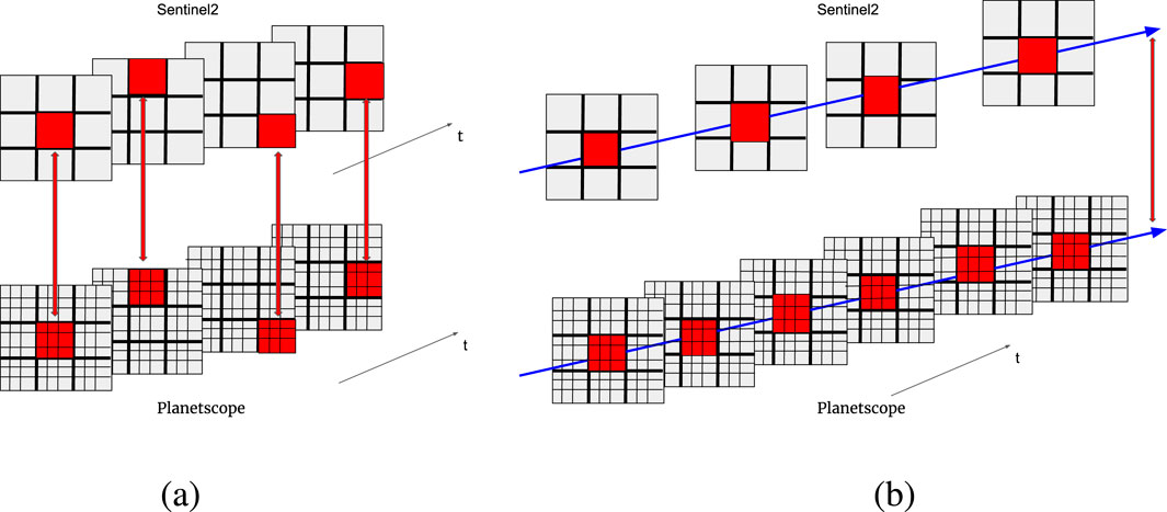
Figure 1. Illustration of the sampling of the pre-training dataset (a) in the baseline model and in the (b) spectro-temporal self-supervised method. In the baseline spectral contrastive method, the spectrally resolved measurements from the same spatial location and the same timestamp are chosen as complementing pairs as indicated by the red lines connecting the pixels. In our new spectro-temporal self-supervised method, the time series of each pixel or group of pixels (shown with blue color) are used as corresponding pairs. In both panels, the top part represents Sentinel-2 and the bottom part represents Planetscope.

The downstream evaluation tasks for crop classification are the same as those used in (Patnala et al., 2024). There are three downstream tasks in total. The downstream task 1 is from the same spatial region (Brandenburg, Germany) as the pre-training dataset from the year 2018. The downstream task 2 is from a different spatial region, albeit still in Brandenburg, and the measurements are from the year 2019. Both downstream tasks 1 and 2 consist of a total of 45,000 training data samples and 9,000 validation data samples each with equal distribution across 9 classes of crops. Figure 2 shows the splitting of the crop fields.

Figure 2

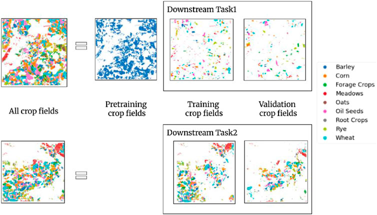
Figure 2. Dataset for the bi-modal self-supervised learning experiment. The top part of the figure illustrates the splitting of crop fields present in the DENETHOR’s training set into 3 different non-overlapping crop fields. The first split shown in the blue color are the crop fields used solely for the purpose of pre-training. The remaining crop fields are used to generate training and validation subset for downstream task 1. Similarly, the bottom row illustrates the splitting of DENETHOR’s validation region into 2 non-overlapping set of crop fields. The two splits are used to generate a training and validation subset for downstream task 2. The figure is taken from Patnala et al. (2024).

In downstream task 3, the measurements are taken from a different region (Brittany, France) from the year 2018. The dataset is a subset of the Breizhcrop dataset (Rußwurm et al., 2019). The dataset provides an aggregated spatial measurement per field parcel. There are 9 crop types in the original dataset (permanent meadows, temporary meadows, corn, wheat, rapeseed, barley, orchards, sunflower, and nuts). The crop fields that contain orchards, sunflowers, and nuts are discarded as there are fewer field parcels for these crop types. Our final downstream task 3 contains 54,000 training data samples and 6,000 validation data samples that are uniformly distributed across 6 classes. In both DENETHOR and Breizhcrops, the crop data provided have a full annual production cycle.

It is important to note that the ratio of training to validation samples for each downstream task is slightly lower than what’s typically used in remote sensing. We employed a 70–30 split in dividing the crop fields, rather than the datasets themselves. For downstream task 1, the ratio of training crop fields to validation crop fields is 21:9, primarily because other crop fields were used for pre-training. For downstream tasks 2 and 3, we maintained the 70:30 ratio. We opted for a higher proportion of training samples to include more data. This approach helps the network learn to recognize and account for pixels located at field borders or significantly affected by cloud cover.

3 Methods

We propose a novel bi-modal BERT-inspired pre-training strategy inspired by the original BERT model (Devlin et al., 2018) for encoding contextual representations of sequential data like text. In the original BERT, a tokenized text from a sentence is passed through the encoder part of a transformer. Before passing it to the encoder, some tokens are masked. Among these masked tokens, some are simply replaced by random values, some are replaced by other values from the distribution, and a few tokens are re-inserted with their original values. Similar to BERT’s masked language modeling approach, we randomly mask timestamps in the Sentinel-2 input sequence before passing it through the transformer encoder.

Our pre-training objective is to predict the corresponding high-resolution Planetscope reflectance values at the masked time steps and spatial locations. For this, the model has to use the contextual information from the unmasked time steps of the Sentinel-2 data. To exploit the finer temporal resolution of Planetscope data, we extend this approach to predict not just the original masked time step, but also the reflectance values for two preceding time steps. This multiple timestamp prediction strategy encourages the model to capture the finer temporal resolution of Planetscope. Since we are dealing with a regression task, the loss function used is the mean squared error (MSE) between the predicted and actual Planetscope reflectance values averaged over the three time steps. Figure 3 illustrates this setup.

Figure 3

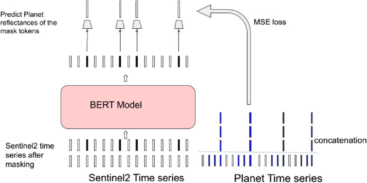
Figure 3. Our model is trained on time series data from Sentinel-2 and PlanetScope. The time series have different spatial and temporal resolutions. In this case, we only illustrate the temporal resolution. A subset of the Sentinel-2 time series is masked and the model is trained to predict the corresponding values of the Planetscope time series. Since Planetscope has a higher temporal resolution, the values of 3 timestamps instead of 1 timestamp are predicted.

We now describe the loss functions that are used for self-supervised learning more in detail. A Sentinel-2 time series with 12 spectral channels is denoted as $x_s=(x_{s1},x_{s2},x_{s3}\dots ,x_{st})$ where $t=144$ and $x_{si}\in {\mathbb{R}}^{12}$. A Planetscope time series is denoted as $x_p=(x_{p1},x_{p2},x_{p3}\dots ,x_{pt})$ where $t=365$ and each time step $x_{pi}\in {\mathbb{R}}^{36}$, where $x_{pi}$ is the concatenation of 4 spectral channels over 9 pixels. Note that Planetscope has a higher spatial and temporal resolution than Sentinel-2 as illustrated in Figure 1. While Patnala et al. (2024) already demonstrated the benefit of using additional data from Planetscope for self-supervised learning although the downstream tasks are only for Sentinel-2 data, we show that our proposed spectro-temporal model, which considers the temporal information over an entire year and includes two novel loss functions that consider seasonal and cloud effects, outperforms (Patnala et al., 2024). Our BERT model is denoted by $F$ and it learns a representation $z$ = $F(x_s)$ for a Sentinel-2 time series with 144 timesteps. Each timestep $z_t\in {\mathbb{R}}^{256}$ is represented by a 256 dimensional vector. Out of the 144 timesteps, we randomly select $90\%$ of the timesteps denoted by $\tilde{T}$. The selected timestamps are then passed to a linear layer $g(z_{si})$ to obtain $y_{si}\in {\mathbb{R}}^{36}$. The corresponding timestamp for Planetscope is denoted as $x_{pi}\in {\mathbb{R}}^{36}$. We then compute the MSE as shown in the Equation 1.

${\mathbb{L}}_{\mathit{bert}}=\frac{1}{2|\tilde{T}|}{\displaystyle \sum _{i\in \tilde{T}}}\Vert y_{si}-x_{pi}{\Vert }^2,(1)$

i.e., we aim to reconstruct the values of the spectral channels of the Planetscope data for the corresponding timestep. Since Planetscope has a higher temporal resolution than Sentinel2, we reconstruct not only 1 timestep but 3. In this case, $y_{si}\in {\mathbb{R}}^{\mathit{3x36}}$ and $x_{pi}\in {\mathbb{R}}^{\mathit{3x36}}$.

To further improve the representation that is learned in our bimodal BERT model, we incorporate two auxiliary losses in parallel, namely seasonal loss and cloud loss. A seasonal classification loss is used to capture phenological nuances across different crop growing seasons. The transformer outputs $z$ are aggregated by month, i.e., $z_m$ for $m\in \{1,\dots ,12\}$, and passed through a linear classifier $h_m$ to predict $c_m$, the class probabilities of each month label $\{1,\dots ,12\}$. We then use the cross-entropy as seasonal loss as per Equation 2:

${\mathbb{L}}_{\mathit{seasonal}}=-\frac{1}{12}{\displaystyle \sum _{m=1}^{12}}\log \left(c_{m,m}\right),(2)$

where $c_{m,m}$ is the predicted probability of the month $m$ for $z_m$. This encourages the model to implicitly learn seasonal patterns that influence crop traits. Figure 4 illustrates the seasonal loss.

Figure 4

Figure 4. Auxiliary seasonal loss.

An additional cloud prediction loss is used to make the model aware of atmospheric distortions and implicitly learn the effect of clouds on the measured reflectance. Cloud measurements are readily available in the Sentinel-2 dataset and discretized into 32 cloud levels. We select a subset of timesteps ${\tilde{T}}_{\mathit{cloud}}$ to directly predict the cloud levels for each timestep $i\in {\tilde{T}}_{\mathit{cloud}}$ using a linear layer with softmax $l_i=h(z_{si})$, where we denote the probability of a cloud level $j$ at timestep $i$ by $l_{i,j}$ and the ground-truth cloud level by ${cl}_i$. As cloud loss, we then use the cross entropy loss as shown in the Equation 3:

${\mathbb{L}}_{\mathit{cloud}}=-\frac{1}{|{\tilde{T}}_{\mathit{cloud}}|}{\displaystyle \sum _{i\in {\tilde{T}}_{\mathit{cloud}}}}{\displaystyle \sum _{j=1}^{32}}{\mathbb{I}}_{j={cl}_i}\log \left(l_{i,j}\right),(3)$

where ${\mathbb{I}}_x$ is the indicator function, which is 1 if $x$ is true and otherwise 0. The loss is illustrated in Figure 5.

Figure 5

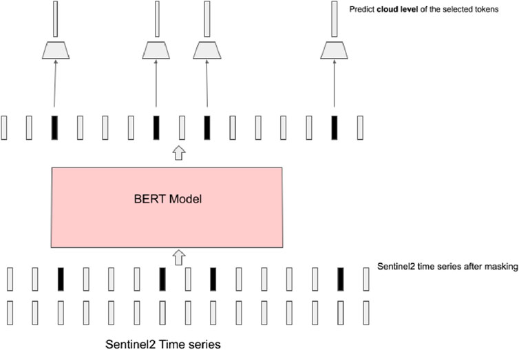
Figure 5. Auxiliary cloud prediction loss.

4 Experiments

As a backbone, we used a transformer model (Dosovitskiy et al., 2020) with 32 layers. Instead of using 2D convolutions in the initial layer, we used 1D convolutions to process the time series data of Sentinel-2. The pre-training objective was to minimize the MSE between the model’s predicted reflectance values and the actual measurements from the Planetscope sensors. For training, we used the following masking. $10\%$ of the tokens were masked to predict the cloud level for the cloud prediction auxiliary task. Another $70\%$ were masked and replaced with random values, $10\%$ were replaced with values sampled from the data distribution, and the remaining $10\%$ were left unchanged. The network was trained for 100 epochs using a batch size of 64. The initial learning rate was set to $10^{-3}$, with a warmup period of 5 epochs. A cosine annealing scheduler was employed to regulate the learning rate during training. The self-supervised trained transformer model provides a contextual time series representation.

For downstream tasks, this contextual time series representation serves as input to various base models: bi-directional long short term memory (LSTM), inceptiontime, and transformer as depicted in Figure 6. To evaluate the effectiveness of our pre-trained model across different model configurations, we randomly generated 10 network instances for each base model type (LSTM, inceptiontime, and transformer) using Optuna (Akiba et al., 2019). For bi-directional LSTM, the hyperparameter space is defined as follows: dimensions of the hidden layer as one of $\{\mathrm{32,64,128,256}\}$, number of layers between 2 and 6, and learning rate in the range from $10^{-5}$ to $10^{-3}$. For inceptiontime, the hyperparameter space is specified as follows: number of layers as either 2, 4, or 8, dimension of hidden layer as one of $\{\mathrm{128,256,512,1024}\}$, kernel size as one of $\{\mathrm{40,80,120,136}\}$, and learning rate between $10^{-5}$ and $10^{-3}$. The hyperparameter space for position encoded transformers is defined as follows: the dimension of the model is either of $\{\mathrm{32,64,128}\}$, the number of attention heads as one of $\{\mathrm{2,4,8}\}$, the number of layers between 2 and 6, and the learning rate ranges between $10^{-5}$ and $10^{-3}$.

Figure 6

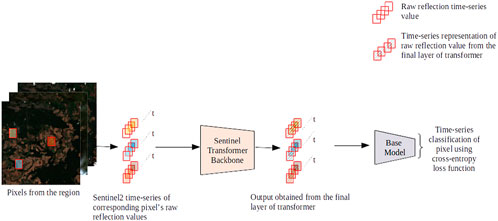
Figure 6. Experiment setup of the crop classification downstream tasks using the pre-trained transformer network. Each pixel is selected and the corresponding time series is then passed to the pre-trained Sentinel transformer. The output of the transformer model is an encoded representation of the time series, which is then passed to the base model for multi-class time series classification.

5 Ablation studies

This section presents an ablation analysis investigating how various parameters affect the performance of both the ResMLP and BERT pre-trained models. We explore the following aspects: impact of number of layers in the ResMLP model (Section 5.1), effect of number of layers in the BERT model (Section 5.2), influence of masking rate on BERT (Section 5.3), comparison between BERT and the spectro-temporal contrastive approach (Section 5.4), and an analysis of the impact of the auxiliary losses for the BERT model, specifically the seasonal classification and cloud prediction losses. Further, in the same subsection, we analyzed the effect of predicting multiple timestamps (Section 5.5). Finally, we examined the effects of different auxiliary losses (Section 5.6).

For all case studies, we report the mean classification accuracy and standard deviation across 10 models with varying hyperparameters (see Section 6). Our results focus on downstream task 2, as described in Section 2. We limit our ablation studies to LSTM and transformer architectures due to the inferior performance observed in inception models.

5.1 Number of layers on ResMLP model

Figure 7 illustrates the effect of increasing the number of layers on the ResMLP model’s performance for both LSTM and Transformer architectures. The mean accuracy increases by increasing the number of layers. Notably, for LSTM models, there is a marginal increment observed when transitioning from 32 to 64 layers.

Figure 7

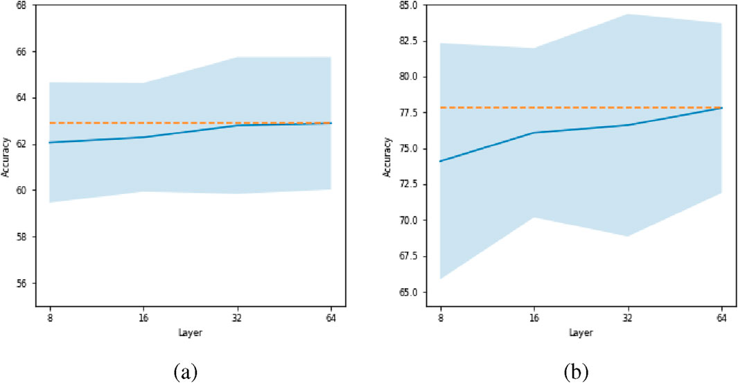
Figure 7. Effect of number of layers for ResMLP model. Plot (a) corresponds to LSTM and plot (b) corresponds to the transformer. The orange dashed line represents the maximum accuracy achieved across varying numbers of layers.

5.2 Effect of number of layers on BERT model

Figure 8 illustrates the effect of increasing the number of layers for the BERT model. We observe improvement for both LSTM and transformer architectures upon increasing the number of layers. To accommodate the larger models on a single GPU, a batch size of 128 was used for the transformer with 16 layers, while a batch size of 64 was used for 32 layers.

Figure 8

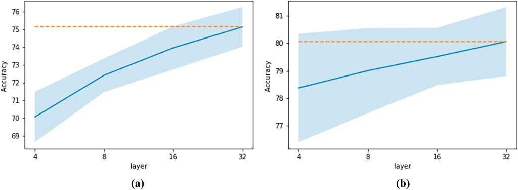
Figure 8. Effect of the number of layers for BERT model. Plot (a) corresponds to LSTM and plot (b) corresponds to transformer. The orange dashed line represents the maximum accuracy achieved across varying numbers of layers.

It is important to note that for the rest of the BERT ablation experiments, a 16-layer transformer architecture was used as the benchmark model for comparing the effects of other parameters and design choices.

5.3 Effect of masking rate on BERT model

Figure 9 illustrates a relationship between the masking rate and its effect on accuracy. For LSTM architectures, we observe an increasing trend in performance as the masking rate is increased from $15\%$ to $90\%$. In the case of Transformer models, the accuracy improves from a $15\%$ masking rate up to $60\%$, after which it plateaus with no significant gains observed at the $90\%$ masking level. The mean difference in accuracy between the $15\%$ and $90\%$ masking rates is approximately $11.01\%$ for LSTM models and $6.84\%$ for transformer models.

Figure 9

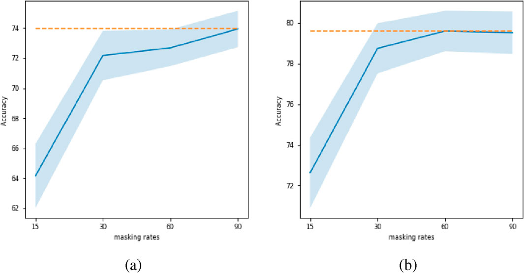
Figure 9. Effect of masking rate for BERT model. Plot (a) corresponds to LSTM and plot (b) corresponds to transformer. The orange dashed line represents the maximum accuracy achieved across different masking rates.

5.4 Comparison between BERT and spectro-temporal contrastive

Spectro-temporal contrastive learning should have been a natural extension of the spectral contrastive method. Instead of utilizing spectral pairs from the same timestamp as complementary views, the spectro-temporal contrastive strategy uses the time series of spectral measurements for each pixel location as the corresponding complementary pair. Figure 10 provides a visual description of our spectro-temporal contrastive method.

Figure 10

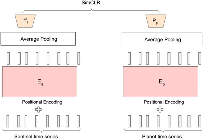
Figure 10. Spectro-temporal contrastive method.

The spectro-temporal contrastive approach has certain drawbacks. This method uses two separate transformer models, which poses a constraint on the maximum batch size. Consequently, we conducted a comparative evaluation between our proposed BERT method and the spectro-temporal contrastive strategy using a smaller transformer architecture, specifically one with 4 layers and an embedding dimension of 64.

Table 1 demonstrates the superiority of BERT over the spectro-temporal contrastive method for both LSTM and transformer. For LSTM, there is a mean overall difference of $15.05\%$ and it is $10.55\%$ for transformer.

Table 1

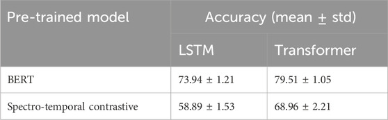
Table 1. Comparison of BERT and spectro-temporal contrastive method when evaluated on LSTM and transformer base models.

5.5 Contribution of auxiliary losses and multiple timestamps

As demonstrated in Table 2, the inclusion of the cloud prediction auxiliary loss results in an overall increase in mean accuracy of $3.88\%$ for LSTM and $2.14\%$ for Transformer models, highlighting the effectiveness of this auxiliary task. Similarly, the addition of the seasonal classifier as an auxiliary loss during pre-training leads to an overall increase in mean accuracy of $6.99\%$ for LSTM and $4.65\%$ for Transformer models, showing the benefits of including seasonal information.

Table 2

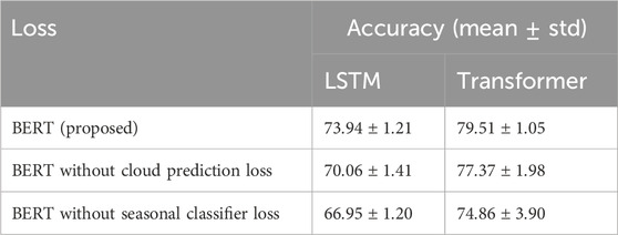
Table 2. Impact of seasonal loss and cloud loss.

Furthermore, Table 3 highlights the advantages of predicting three future time steps during pre-training over predicting a single time step. This results in an overall increase in mean accuracy of $6.27\%$ for LSTM and $3.74\%$ for Transformer models.

Table 3

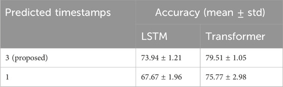
Table 3. Impact of the number of predicted timestamps.

5.6 Comparison between different types of auxiliary loss functions

We compared our proposed cross-entropy loss for the auxiliary task to the mean square loss. Table 4 demonstrates the superiority of the cross-entropy loss over the use of the MSE loss for the auxiliary task. For LSTM, there is a mean overall difference of $3.62\%$ and it is $3.55\%$ for transformer.

Table 4

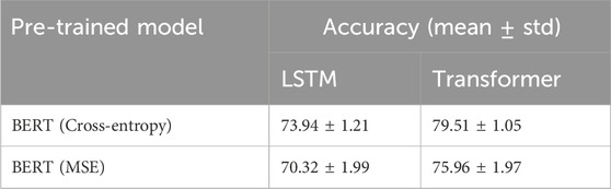
Table 4. Comparison between different losses for the auxiliary task on BERT model when evaluated on LSTM and transformer base model.

6 Results

We compare our proposed spectro-temporal BERT model with a contrastive learning baseline that uses datasets with different spatial resolutions, but does not rely on temporal information for self-supervised learning, as illustrated in Figure 1. The baseline ResMLP (Patnala et al., 2024) consists of 64 layers and was trained with a batch size of 2048. For comparison, we use comparison plots and absolute gain in performance. In the comparison plot, the x-axis presents the accuracy of the ResMLP model and the y-axis represents the accuracy of the BERT model for self-supervised learning. The dotted line across the plot represents a break-even line. Points above the diagonal break-even line, plotted in red, indicate BERT’s superiority over ResMLP, while green points below the line indicate inferior performance. In the plot, we also report the fractional win score (Equation 4), calculated as the number of times out of 10 experiments that BERT surpassed the ResMLP model, i.e.,

$Win\text{\_}score=\frac{{\sum }_{i=1}^N\mathbb{I}\left(ac{c}_{\mathit{BERT}}>ac{c}_{\mathit{ResMLP}}\right)}{N}.(4)$

Figures 11–13 present the comparison plots evaluating the competitive pre-trained models across downstream tasks 1, 2, and 3, respectively. A separate evaluation is done for each base model, i.e., LSTM, inception, and transformer. Since 10 different hyperparameter configurations are employed for each base model, the number of experiments is 10.

Figure 11

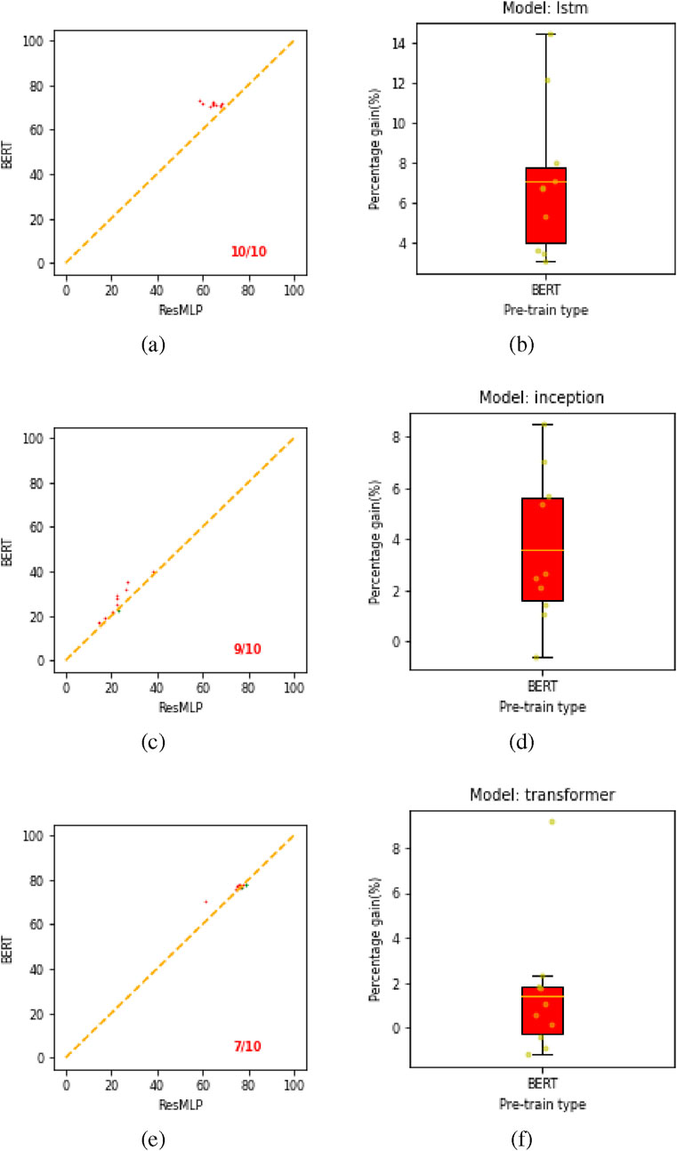
Figure 11. Comparison and box plot for all pre-trained models on downstream task 1. Plots (a,c,e) show the comparison plots for LSTM, inception, and transformer, respectively. Panels (b,d,f) correspond to box plots showing an absolute gain for our proposed BERT model over the ResMLP pre-trained model.

Figure 11 presents the comparison and box plots comparing the performance of our proposed BERT model against the ResMLP baseline for downstream task 1. The win-ratios, indicating the number of times (out of 10 experiments) BERT surpassed ResMLP, are $10/10$ for LSTM, $9/10$ for inception, and $7/10$ for transformer models. The mean classification accuracies achieved by ResMLP models are $64.43\%\pm 3.06\%$ for LSTM, $23.41\%\pm 6.18\%$ for inception, and $75.20\%\pm 4.76\%$ for transformer models. For LSTM, the mean gain of BERT over the ResMLP is 7.04% (min: 3.02%, max: 14.46%). In the case of inception, the mean gain is 3.57% (−0.62%, 8.49%). For transformers, the mean gain is 1.44% (−1.21%, 9.18%).

Figure 12 presents the comparing results for downstream task 2. The win-ratios are $10/10$, $10/10$, and $6/10$ for LSTM, inception, and transformer, respectively. The mean classification accuracies achieved by ResMLP models are $62.88\%\pm 2.86\%$ for LSTM, $22.01\%\pm 4.28\%$ for inception, and $77.80\%\pm 5.92\%$ for transformer. For LSTM, the mean gain of BERT over the ResMLP is $12.24\%$ ($8.68\%$, $19.75\%$). In the case of inception, the mean gain is $12.28\%$ ($9.05\%$, $15.98\%$). For transformers, the mean gain is $2.26\%$ ($-3.27\%$, $13.54\%$).

Figure 12

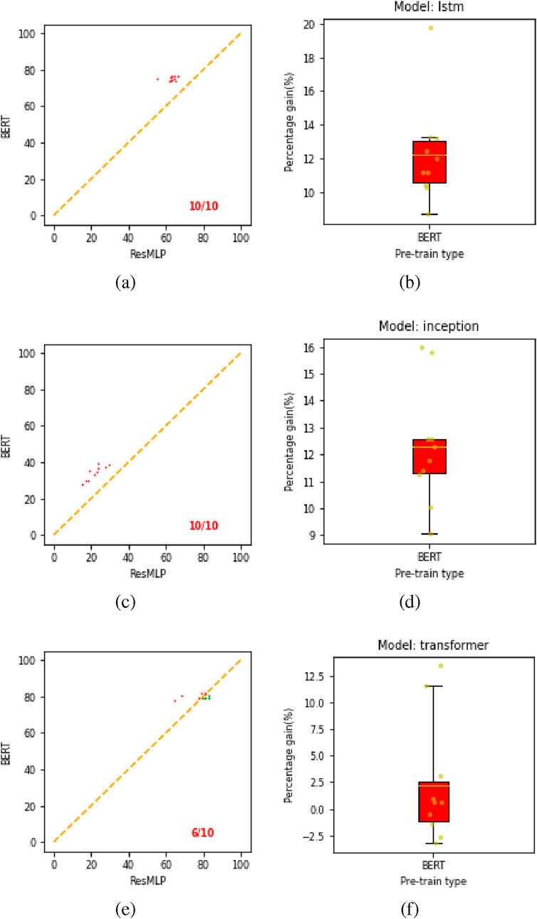
Figure 12. Comparison plot and box plot for all pre-trained models on downstream task 2. Plots (a,c,e) show the comparison plots for LSTM, inception, and transformer, respectively. Panels (b,d,f) correspond to box plots showing absolute gain for our proposed BERT model over the ResMLP pre-trained model.

Figure 13 presents the results for downstream task 3. The win-ratios are $3/10$ for LSTM, $9/10$ for inception, and $6/10$ for transformer. The mean classification accuracy achieved by the ResMLP models is $56.32\%\pm 0.47\%$ for LSTM, $16.37\%\pm 5.97\%$ for inception, and $53.87\%\pm 2.82\%$ for transformer. For LSTM, the mean gain of BERT over the ResMLP is $-0.11\%$ ($-0.70\%$, $0.56\%$). It is the only setting where BERT performs on average worse than ResMLP. In the case of inception, the mean gain is $5.91\%$ ($-3.47\%$, $18.59\%$). For transformers, the mean gain is $1.15\%$ ($-2.05\%$, $6.93\%$) for BERT.

Figure 13

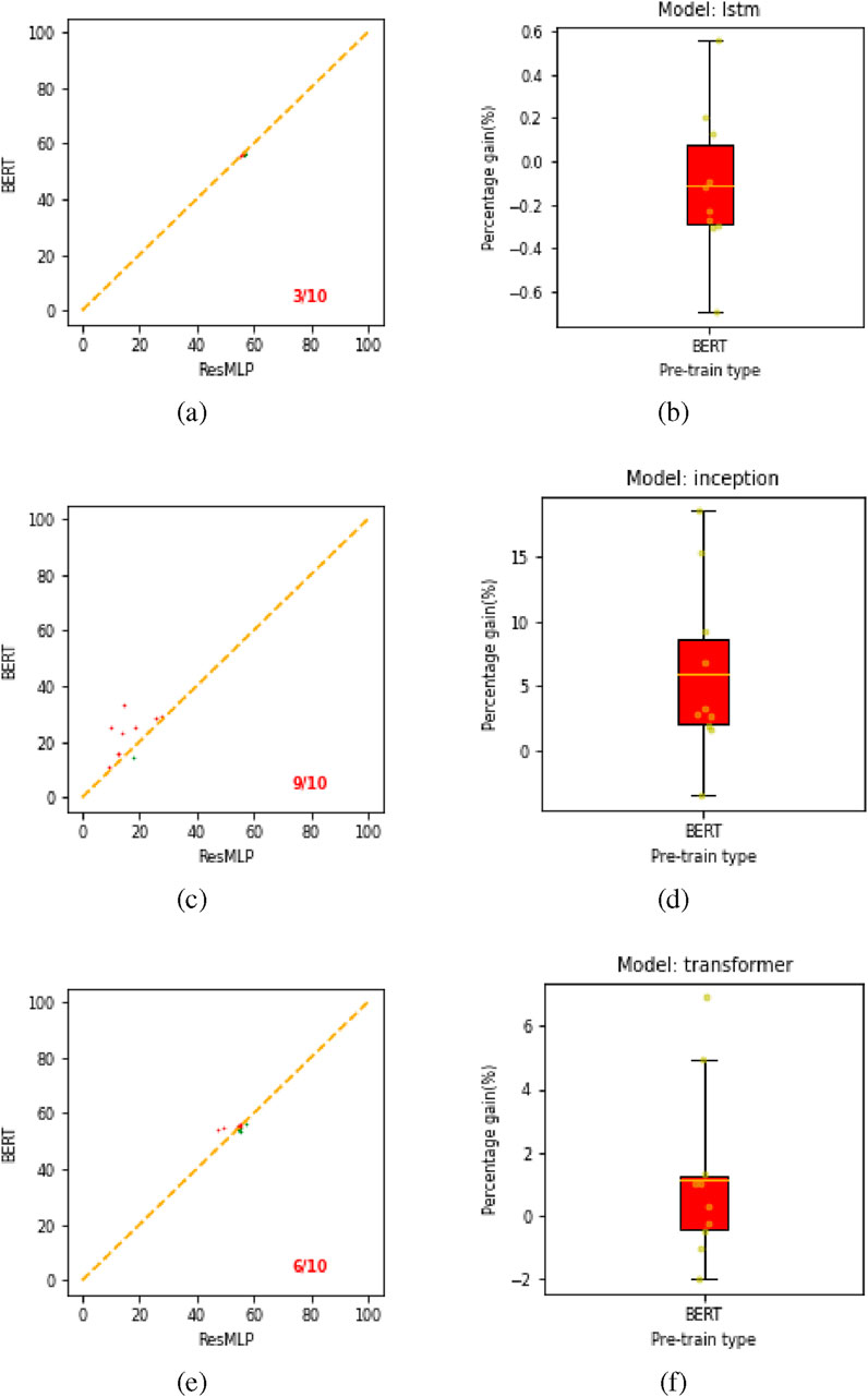
Figure 13. Win-matrix and box plot for all pre-trained models on downstream task 3. Plots (a,c,e) show the win-matrix for LSTM, inception, and transformer, respectively. Panels (b,d,f) correspond to box plots showing an absolute gain for our proposed BERT model over the ResMLP pre-trained model.

Table 5 presents the classification accuracy achieved by models trained using the representations learned from the ResMLP self-supervised approach and our proposed BERT bimodal method across all three downstream crop classification tasks.

Table 5

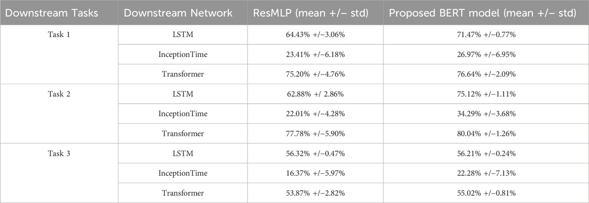
Table 5. Accuracy of the models for both pre-trained ResMLP self-supervised model and our proposed BERT model in three different downstream tasks.

Based on the experimental results presented, the proposed bi-modal BERT approach demonstrates consistent performance gains over the baseline ResMLP method across the three downstream crop classification tasks and different base model architectures (LSTM, InceptionTime, Transformer). For LSTM architectures, the BERT approach is clearly superior on downstream tasks 1 and 2. On task 3, there is no improvement and the performance is comparable to ResMLP, with most model configurations lying close to the break-even line as shown in Figure 13. In the case of transformer models, the BERT method consistently outperforms ResMLP across all tasks. Figures 14, 15 present maps that compare the performance of the BERT model against the ResMLP baseline model. These maps specifically illustrate the results for one configuration on downstream task 2. The plots from different configurations showed similar results. We present results from downstream task 2 because its data is relatively similar to the data used for pre-training, unlike the data in downstream task 3. Also, the data for downstream task 1 is from the same region and time, so it does not provide enough variability.

Figure 14

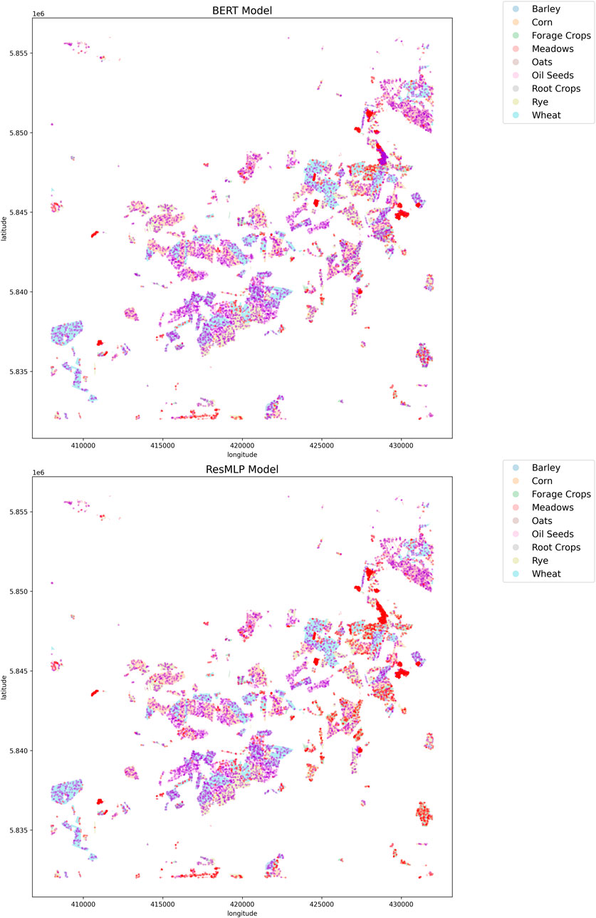
Figure 14. Visualization of the crop classification map for both spectral-temporal BERT and ResMLP pre-trained model. Dark violet points indicate where the predictions are correct, and red points show where predictions are wrong. The results are from the LSTM model evaluated on the validation set of downstream task 2. Out of 10 available hyperparameter configurations, these results were obtained using hyperparameters corresponding to model number 5.

Figure 15

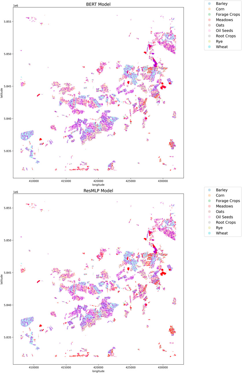
Figure 15. Visualization of the crop classification map for both spectral-temporal BERT and ResMLP pre-trained model. Dark violet points indicate where the predictions are correct, and red points show where predictions are wrong. The results are from the transformer model evaluated on the validation set of downstream task 2. Out of 10 available hyperparameter configurations, these results were obtained using hyperparameters corresponding to model number 5.

In summary, the proposed spectro-temporal BERT method outperforms the ResMLP baselines in 8 out of 9 cases and it is on par in one case. By using very different architectures for the time series classification with 10 different hyper-parameters each, we showed that the results generalize across different architectures. The results show the advantage of a temporal model compared to a contrastive learning approach. Note that both the proposed spectro-temporal BERT model and ResMLP utilize data from different sources with different spatial and temporal resolutions, namely Sentinel-2 and Planetscope, but only our approach leverages the higher temporal resolution of Planetscope.

7 Discussion

We have demonstrated the advantages of employing spectro-temporal self-supervised methods over those that solely utilize spectral components. The BERT approach offers a key benefit over its spectro-temporal contrastive counterpart: it requires only one transformer model during training and can be easily scaled across multiple devices using data-distributed parallelism techniques (Li et al., 2020). While alternative loss functions to contrastive loss exist, such as Barlow twins (Zbontar et al., 2021), studies like (Bahri et al., 2021; Patnala et al., 2024) have shown that these alternatives fail to yield superior representations for tabular data. Other loss functions, including MoCo (He et al., 2019), DiNo (Caron et al., 2021), and BYOL (Grill et al., 2020), employ momentum-based distillation techniques, thus making them less adaptable to multi-modal setups. Our transformer model takes roughly 20 h to train for 100 epochs on V100 GPUs, mainly due to our selection of a higher number of layers and a large dimension for the intermediate MLP layer. However, the ResMLP model, with an equivalent number of layers and hidden dimensions, exhibits similar training times. It is worth noting that the transformer has a computational complexity of $O(N^2)$. In our experimental setup, we use 144 time stamps as tokens, which mitigates the impact of this complexity. Emerging state space models like MAMBA (Gu and Dao, 2024) show promise in competing with transformers, offering both convolutional and recurrent setups for faster training and inference, respectively. Such models are beginning to gain traction in the remote sensing community (Huang et al., 2024). The limitations of our approach are as follows: Our pre-training process uses a regional dataset that focuses specifically on croplands in a small area of Brandenburg. This limited geographical scope restricts the model’s ability to generalize to other regions, particularly in developing areas where labeled data is scarce. The model’s performance can be improved by expanding the pre-training dataset to include samples from a wider range of geographic locations. This expansion would allow the model to learn more diverse crop patterns and potentially make it more suitable for use in developing countries where fewer labeled examples are available. In fact, it would be highly beneficial, if a large multi-sensor dataset encompassing several world regions were made available to the community so that larger, more powerful unsupervised machine learning models can be trained and evaluated. Such community datasets were very influential in several other domains. In this study, we utilized data from DENETHOR and Breizhcrop, where the crop data covers a complete annual production cycle. However, if crops with varying annual cycles are involved, systematic batching or modern GPUs equipped with flash attention would be required. Flash attention enables efficient processing of variable-length data within a single batch, making it suitable for such scenarios. Additionally, our current approach uses a 3 $\times$ 3 set of pixels for Planetscope without considering larger spatial contexts. Recent works like UBARN (Dumeur et al., 2024b) and ALISE (Dumeur et al., 2024a) have explored BERT-style training in the spatio-spectro-temporal domain, albeit using a single source. A promising future direction would be to investigate how our multi-modal strategy could be applied to such models.

8 Conclusion

In this study, we extended the work of Patnala et al. (2024) by introducing an innovative bi-modal approach that combines spectral and temporal data from two satellites for self-supervised pre-training and by adopting a BERT-style training strategy. We tested this method on three distinct downstream tasks related to crop classification. Our methodology draws inspiration from the BERT model, but it is adapted to predict Planetscope reflectance values from Sentinel-2 data. Our model leverages the higher spectral information of Sentinel-2 data and Planetscope’s higher spatial and temporal resolution. We also developed two new loss functions for self-supervised learning. The seasonal classifier loss enhances the model’s ability to differentiate between seasons, while the cloud prediction task utilizes metadata to inform the model about cloud coverage in pixels at specific times, allowing it to implicitly understand cloud-related distortions in reflectance readings. As evidenced by the results in Section 6, our BERT bi-modal model consistently outperformed the ResMLP model across most test scenarios, and it performed comparably in the other test scenarios. This suggests that our BERT approach, pre-trained on combined spectro-temporal information and enhanced with auxiliary seasonal and cloud prediction losses, learns representations that are highly effective for crop classification. We anticipate that this approach is scalable and that the model’s performance could further improve with larger training datasets.

Data availability statement

Publicly available datasets were analyzed in this study. This data can be found here: https://github.com/lukaskondmann/DENETHOR.

Author contributions

AP: Conceptualization, Data curation, Methodology, Project administration, Software, Writing – original draft, Writing – review and editing. MS: Supervision, Validation, Writing – review and editing. JG: Supervision, Validation, Writing – review and editing.

Funding

The author(s) declare that financial support was received for the research and/or publication of this article. The research was funded by German Federal Ministry for the Environment, Nature Conservation, and Nuclear Safety under grant no 67KI 2043 (KISTE). Computing time for this study was kindly provided by the Juelich Supercomputing Centre under project DeepACF. JG is supported by the Deutsche Forschungsgemeinschaft (DFG, German Research Foundation) - SFB 1502/1-2022 - Projektnummer:450058266.

Acknowledgments

We acknowledge the support from Michael Langguth in proofreading the paper.

Conflict of interest

The authors declare that the research was conducted in the absence of any commercial or financial relationships that could be construed as a potential conflict of interest.

Generative AI statement

The author(s) declare that Generative AI was used in the creation of this manuscript. The perplexity standard version was used to rephrase the text and look into grammatical errors.

Publisher’s note

All claims expressed in this article are solely those of the authors and do not necessarily represent those of their affiliated organizations, or those of the publisher, the editors and the reviewers. Any product that may be evaluated in this article, or claim that may be made by its manufacturer, is not guaranteed or endorsed by the publisher.

Footnotes

¹https://api.planet.com

References

Akiba, T., Sano, S., Yanase, T., Ohta, T., and Koyama, M. (2019). Optuna: a next-generation hyperparameter optimization framework. Corr. abs/1907, 10902. doi:10.1145/3292500.3330701

CrossRef Full Text | Google Scholar

Ayush, K., Uzkent, B., Meng, C., Tanmay, K., Burke, M., Lobell, D. B., et al. (2020). Geography-aware self-supervised learning. Corr. abs/2011, 09980. doi:10.48550/arXiv.2011.09980

CrossRef Full Text | Google Scholar

Bahri, D., Jiang, H., Tay, Y., and Metzler, D. (2021). SCARF: self-supervised contrastive learning using random feature corruption. Corr. abs/2106 (15147). doi:10.48550/arXiv.2106.15147

CrossRef Full Text | Google Scholar

Bharti, S., Kaur, P., Singh, P., Madhu, C., and Garg, N. (2022). “Crop yield prediction using cnn-lstm model,” in 2022 IEEE conference on interdisciplinary approaches in technology and management for social innovation (IATMSI), 1–5. doi:10.1109/IATMSI56455.2022.10119308

CrossRef Full Text | Google Scholar

Brown, T. B., Mann, B., Ryder, N., Subbiah, M., Kaplan, J., Dhariwal, P., et al. (2020). Language models are few-shot learners. Corr. abs/2005, 14165. doi:10.48550/arXiv.2005.14165

CrossRef Full Text | Google Scholar

Caron, M., Touvron, H., Misra, I., Jégou, H., Mairal, J., Bojanowski, P., et al. (2021). Emerging properties in self-supervised vision transformers. Corr. abs/2104 (14294). doi:10.1109/ICCV48922.2021.00951

CrossRef Full Text | Google Scholar

Cecili, G., De Fioravante, P., Dichicco, P., Congedo, L., Marchetti, M., and Munafò, M. (2023). Land cover mapping with convolutional neural networks using sentinel-2 images: case study of rome. Land 12, 879. doi:10.3390/land12040879

CrossRef Full Text | Google Scholar

Chen, T., Kornblith, S., Norouzi, M., and Hinton, G. E. (2020). A simple framework for contrastive learning of visual representations. CoRR, 05709. doi:10.48550/arXiv.2002.05709

CrossRef Full Text | Google Scholar

Lessig, C., Luise, I., Gong, B., Langguth, M., Stadtler, S., and Schultz, M. (2023). Atmorep: a stochastic model of atmosphere dynamics using large scale representation learning.

Google Scholar

Dell’Acqua, F., Iannelli, G. C., Torres, M. A., and Martina, M. L. (2018). A novel strategy for very-large-scale cash-crop mapping in the context of weather-related risk assessment, combining global satellite multispectral datasets, environmental constraints, and in situ acquisition of geospatial data. Sensors 18, 591. doi:10.3390/s18020591

PubMed Abstract | CrossRef Full Text | Google Scholar

Devlin, J., Chang, M., Lee, K., and Toutanova, K. (2018). BERT: pre-training of deep bidirectional transformers for language understanding. Corr. abs/1810, 04805. doi:10.48550/arXiv.1810.04805

CrossRef Full Text | Google Scholar

Dosovitskiy, A., Beyer, L., Kolesnikov, A., Weissenborn, D., Zhai, X., Unterthiner, T., et al. (2020). An image is worth 16x16 words: transformers for image recognition at scale. Corr. abs/2010, 11929. doi:10.48550/arXiv.2010.11929

CrossRef Full Text | Google Scholar

Drusch, M., Del Bello, U., Carlier, S., Colin, O., Fernandez, V., Gascon, F., et al. (2012). Sentinel-2: esa’s optical high-resolution mission for gmes operational services. Remote Sens. Environ. 120, 25–36. doi:10.1016/j.rse.2011.11.026

CrossRef Full Text | Google Scholar

Dumeur, I., Valero, S., and Inglada, J. (2024a). Paving the way toward foundation models for irregular and unaligned Satellite Image Time Series.

Google Scholar

Dumeur, I., Valero, S., and Inglada, J. (2024b). Self-supervised spatio-temporal representation learning of satellite image time series. IEEE J. Sel. Top. Appl. Earth Observations Remote Sens. 17, 4350–4367. doi:10.1109/JSTARS.2024.3358066

CrossRef Full Text | Google Scholar

Garnot, V. S. F., and Landrieu, L. (2021). Panoptic segmentation of satellite image time series with convolutional temporal attention networks. Corr. abs/2107, 07933. doi:10.48550/arXiv.2107.07933

CrossRef Full Text | Google Scholar

Grill, J., Strub, F., Altché, F., Tallec, C., Richemond, P. H., Buchatskaya, E., et al. (2020). Bootstrap your own latent: a new approach to self-supervised learning. Corr. abs/2006 (07733). doi:10.48550/arXiv.2006.07733

CrossRef Full Text | Google Scholar

Gu, A., and Dao, T. (2024). Mamba: linear-time sequence modeling with selective state spaces

Google Scholar

Gui, J., Chen, T., Zhang, J., Cao, Q., Sun, Z., Luo, H., et al. (2024). A survey on self-supervised learning: algorithms, applications, and future trends. IEEE Trans. Pattern Analysis and Mach. Intell. 46, 9052–9071. doi:10.1109/TPAMI.2024.3415112

PubMed Abstract | CrossRef Full Text | Google Scholar

He, K., Fan, H., Wu, Y., Xie, S., and Girshick, R. B. (2019). Momentum contrast for unsupervised visual representation learning. Corr. abs/1911, 05722. doi:10.48550/arXiv.1911.05722

CrossRef Full Text | Google Scholar

He, K., Zhang, X., Ren, S., and Sun, J. (2015). Deep residual learning for image recognition. Corr. abs/1512, 03385. doi:10.48550/arXiv.1512.03385

CrossRef Full Text | Google Scholar

Huang, G., Liu, Z., and Weinberger, K. Q. (2016). Densely connected convolutional networks. Corr. abs/1608, 06993. doi:10.48550/arXiv.1608.06993

CrossRef Full Text | Google Scholar

Huang, L., Chen, Y., and He, X. (2024). Spectral-spatial mamba for hyperspectral image classification. Remote Sens. 16, 2449. doi:10.3390/rs16132449

CrossRef Full Text | Google Scholar

Hütt, C., Waldhoff, G., and Bareth, G. (2020). Fusion of sentinel-1 with official topographic and cadastral geodata for crop-type enriched lulc mapping using foss and open data. ISPRS Int. J. Geo-Information 9, 120. doi:10.3390/ijgi9020120

CrossRef Full Text | Google Scholar

Khan, M., Hanan, A., Kenzhebay, M., Gazzea, M., and Arghandeh, R. (2024). Transformer-based land use and land cover classification with explainability using satellite imagery. Sci. Rep. 14, 16744. doi:10.1038/s41598-024-67186-4

PubMed Abstract | CrossRef Full Text | Google Scholar

Kondmann, L., Toker, A., Rußwurm, M., Camero, A., Peressuti, D., Milcinski, G., et al. (2021). “DENETHOR: the dynamicearthNET dataset for harmonized, inter-operable, analysis-ready, daily crop monitoring from space,” in Thirty-fifth conference on neural information processing systems datasets and benchmarks track (round 2).

Google Scholar

Li, S., Zhao, Y., Varma, R., Salpekar, O., Noordhuis, P., Li, T., et al. (2020). Pytorch distributed: experiences on accelerating data parallel training. Corr. abs/2006, 15704. doi:10.48550/arXiv.2006.15704

CrossRef Full Text | Google Scholar

Luo, J., Xie, M., Wu, Q., Luo, J., Gao, Q., Shao, X., et al. (2024). Early crop identification study based on sentinel-1/2 images with feature optimization strategy. Agriculture 14, 990. doi:10.3390/agriculture14070990

CrossRef Full Text | Google Scholar

Meier, U., Bleiholder, H., Buhr, L., Feller, C., Hack, H., Heß, M., et al. (2009). The bbch system to coding the phenological growth stages of plants-history and publications. J. für Kulturpflanzen 61, 41–52. doi:10.5073/JfK.2009.02.01

CrossRef Full Text | Google Scholar

Patnala, A., Stadtler, S., Schultz, M. G., and Gall, J. (2024). Bi-modal contrastive learning for crop classification using Sentinel-2 and Planetscope. Front. Remote Sens. 5, 1480101. doi:10.3389/frsen.2024.1480101

CrossRef Full Text | Google Scholar

Purushwalkam, S., and Gupta, A. (2020). “Demystifying contrastive self-supervised learning: invariances, augmentations and dataset biases,” in Advances in neural information processing systems 33: annual conference on neural information processing systems 2020, NeurIPS 2020, december 6-12, 2020, virtual.

Google Scholar

Račič, M., Oštir, K., Peressutti, D., Zupanc, A., and Čehovin Zajc, L. (2020). Application of temporal convolutional neural network for the classification of crops on sentinel-2 time series. ISPRS - Int. Archives Photogrammetry, Remote Sens. Spatial Inf. Sci. XLIII-B2-2020, 1337–1342. doi:10.5194/isprs-archives-XLIII-B2-2020-1337-2020

CrossRef Full Text | Google Scholar

Rad, R. (2024). “Vision transformer for multispectral satellite imagery: advancing landcover classification,” in Proceedings of the IEEE/CVF winter conference on applications of computer vision (WACV), 8176–8183.

Google Scholar

Ray, D. K., Sloat, L. L., Garcia, A. S., Davis, K. F., Ali, T., and Xie, W. (2022). Crop harvests for direct food use insufficient to meet the un’s food security goal. Nat. Food 3, 367–374. doi:10.1038/s43016-022-00504-z

PubMed Abstract | CrossRef Full Text | Google Scholar

Rußwurm, M., Lefèvre, S., and Körner, M. (2019). Breizhcrops: a satellite time series dataset for crop type identification. Corr. abs/1905, 11893. doi:10.48550/arXiv.1905.11893

CrossRef Full Text | Google Scholar

Scheibenreif, L., Hanna, J., Mommert, M., and Borth, D. (2022). “Self-supervised vision transformers for land-cover segmentation and classification,” in IEEE/CVF conference on computer vision and pattern recognition workshops, CVPR workshops 2022, New Orleans, LA, USA, june 19-20, 2022 (IEEE), 1421–1430. doi:10.1109/CVPRW56347.2022.00148

CrossRef Full Text | Google Scholar

Simonyan, K., and Zisserman, A. (2015). Very deep convolutional networks for large-scale image recognition

Google Scholar

Tarasiou, M., Chavez, E., and Zafeiriou, S. (2023). “Vits for sits: vision transformers for satellite image time series,” in Proceedings of the IEEE/CVF conference on computer vision and pattern recognition (CVPR), 10418–10428.

Google Scholar

Yao, J., Zhang, B., Li, C., Hong, D., and Chanussot, J. (2023). Extended vision transformer (exvit) for land use and land cover classification: a multimodal deep learning framework. IEEE Trans. Geoscience Remote Sens. 61, 1–15. doi:10.1109/TGRS.2023.3284671

CrossRef Full Text | Google Scholar

Zbontar, J., Jing, L., Misra, I., LeCun, Y., and Deny, S. (2021). Barlow twins: self-supervised learning via redundancy reduction. Corr. abs/2103, 03230. doi:10.48550/arXiv.2103.03230

CrossRef Full Text | Google Scholar