Average optical path length estimation in a slab of arbitrary finite thickness

A method for determining the average photon path length in a slab of multiple scattering material is presented. Radiances can be obtained from the radiative transfer equation and subsequently differentiated to obtain the average photon path length. These radiances can be obtained via multiple methods including Monte Carlo simulations, analytic two-stream approximations, and multi-stream numerical solutions such as the AccuRT computational tool. Average path lengths obtained via numerical differentiation of these radiances are found to agree closely with path length estimates predicted by existing methods found in the literature. The average photon path length is further considered for a slab of finite physical thickness. It was found that for a slab consisting of non-absorbing material there is a linear relationship between the slab thickness and the average photon path length, but that for materials with nonzero absorption, this linear relationship breaks down as the slab thickness increases. Average path lengths may be converted to time spans to determine the amount of time a photon spends in a multiple scattering medium, which may be used to quantify the impact of multiple scattering on pulse stretching in lidar/radar applications.

1 Introduction

We present a method for computing the average optical path length of photons undergoing random walks in a slab of arbitrary physical thickness. The slab is assumed to consist of a dilute medium¹ with arbitrary values of the single-scattering albedo and the scattering phase function. This method can be used to compute the average optical path length $⟨L_{\text{opt}}⟩$ at any location in the slab, but also to quantify $⟨L_{\text{opt}}⟩$ for photons escaping from the top or bottom of the slab.

The average optical path length $⟨L_{\text{opt}}⟩$ is of interest in a variety of practical applications, such as in the study of the horizontal variability of clouds or in the study of diffuse light transport with relevance to biomedical imaging. In many studies of atmospheric scattering, a plane-parallel atmosphere is assumed with no variability in the horizontal direction. In contrast, Stephens and Heidinger (Stephens and Heidinger, 2000) considered the effects of a three-dimensional cloud geometry. They noted that horizontal cloud heterogeneity may lead to a reduced reflected radiance, which in turn may lead to a corresponding reduced value of the inferred optical depth compared to the optical-depth value obtained in the case of a plane-parallel atmosphere (Stephens and Heidinger, 2000). They further noted that the average photon path length can be used to estimate the optical depth, but that horizontal heterogeneity causes a positive bias as compared to the optical depth values expected in the plane-parallel case. The difference between these two optical depth estimates may be used as a metric to quantify the degree of horizontal heterogeneity of a scattering atmosphere.

The average optical path length $⟨L_{\text{opt}}⟩$ has also been used in the study of diffuse light transport, which has applications in biomedical imaging of strongly scattering biological tissues. For example, Pierrat et al. (2008) used the transport mean free path of photons to determine the regime of validity for the diffusion approximation. At large length scales, the diffusion approximation produces good results for the transport of the diffuse intensity (or radiance). However, the diffusion approximation has limitations at short length scales. Pierrat et al. (2008) investigated these limitations and proposed improved models. Elaloufi et al. (2004) used the transport mean free path to study the dynamic transport of light in optically thin slabs. They found diffusion-approximation results to accurately predict the long-time behavior of transmitted pulses in slabs of physical thickness $h$ larger than $8{\ell }_{tr}$ where ${\ell }_{tr}$ is the transport mean free path. Optically thin slabs $(h<8{\ell }_{tr})$, instead fall into the non-diffusive regime, and the authors used the radiative transfer equation to study the transition from the diffusive to the non-diffusive regime (Elaloufi et al., 2004).

Also, the average optical path length is useful in satellite remote sensing, wherein an instrument such as a lidar deployed in space measures the upward radiance of photons at the top of the atmosphere (TOA). Here the atmosphere may be assumed to be a plane-parallel, horizontal slab varying only with altitude $z$, and satellite remote sensing data may be used to infer the average path length of the photons escaping at the TOA. Likewise, photons emerging from the bottom of the slab, may be used to compute average path lengths that will be useful for interpreting data from ground-based lidar deployments aimed at studying cloud and aerosol properties.

To demonstrate the validity of our method for computing average optical path lengths, we use the AccuRT software tool (Stamnes et al., 2018). This software tool solves the radiative transfer equation (RTE) for two coupled slabs with different refractive indices (such as the coupled atmosphere-ocean system) using the discrete ordinate method. Solutions to the RTE yield radiances at a number of discrete polar quadrature angles (also known as streams), with a greater number of streams producing more accurate results (Stamnes et al., 2017). From these solutions at the polar quadrature angles, the source function can be computed via interpolation of the radiances computed at the polar quadrature angles and then integrated to obtain radiances at arbitrary polar angles by the “integration of the source function technique” as summarized in Section 3.

Prior work has been done in computing the average optical path length from radiance values for some simple cases, as summarized by van de Hulst (Hendrik Christoffel et al., 1980). It is therefore interesting to compare results obtained using our method for computing average optical path lengths, with corresponding results obtained by van de Hulst’s approach.

2 Methodology

Consider a horizontal slab of physical thickness $h$ and inherent optical properties (IOPs) that are characterized by the absorption coefficient $\alpha (z)$, the scattering coefficient $\beta (z)$, and the scattering phase function $p(z,\mathrm{\Theta })$, where $z=0$ at the bottom of the slab and $z=h$ at the top of the slab. The scattering angle $\mathrm{\Theta }$ is related to the polar and azimuth angles $({\theta }^{\prime },{\varphi }^{\prime })$ before a scattering event and $(\theta ,\varphi )$ after a scattering event by the cosine law of spherical trigonometry

$\cos \mathrm{\Theta }=\cos {\theta }^{\prime }\cos \theta +\sin {\theta }^{\prime }\sin \theta \cos \left({\varphi }^{\prime }-\varphi \right).(1)$

The quantity $\gamma (z)=\alpha (z)+\beta (z)$, is called the extinction coefficient and is used to describe the total attenuation or extinction due to the combined effects of absorption and scattering. The single-scattering albedo (SSA), denoted $\varpi (z)=\beta (z)/(\alpha (z)+\beta (z))$, describes the fraction of the extinction that is due to scattering. Note that for a homogeneous slab the scattering and absorption coefficients as well as the scattering phase function do not depend on altitude $z$ measured upwards from the bottom of the slab.

Both the slab thickness $h$ and the inherent optical properties impact the degree to which light is absorbed and multiply scattered. It is convenient to use the slab total optical thickness ${\tau }^{*}=h(\alpha +\beta )$ together with the single-scattering albedo $\varpi =\beta /(\alpha +\beta )$ and the scattering phase function $p(\mathrm{\Theta })$ to encapsulate all required information for a homogeneous slab.

Similarly, if we want to evaluate radiances at some intermediate depth $z$ (with $0\le z\le h$) for a homogeneous slab, we can use the optical depth $\tau (z)=z(\alpha +\beta )$.²

We may also consider the case where some absorbing gas with absorption coefficient $\kappa$ is mixed with small particles which can be characterized using IOPs as just described. We can introduce the parameter

$\eta =\kappa /\left(\alpha +\beta \right)(2)$

which is simply the ratio of the gas absorption coefficient $\kappa$ to the “particulate matter” extinction coefficient $(\alpha +\beta )$.

In such a mixture it is possible to introduce modified values for the optical thickness ${\tau }^{*\prime }={\tau }^{*}(1+\eta )$, optical depth ${\tau }^{\prime }=\tau (1+\eta )$, and single-scattering albedo ${\varpi }^{\prime }=\varpi /(1+\eta )$. That is, for any particulate medium that is mixed with or embedded in an absorbing gas, we may replace the mixture with an equivalent medium in which there is no gas between the particles and where the optical properties of the particles are $({\varpi }^{\prime },{\tau }^{*\prime },{\tau }^{\prime })$ instead of $(\varpi ,{\tau }^{*},\tau )$. This relation is known as the equivalence theorem (Hendrik Christoffel et al., 1980):

$I\left(\tau ,\varpi ,{\tau }^{*},\eta \right)=I\left({\tau }^{\prime },{\varpi }^{\prime },{\tau }^{*\prime }\right)(3)$

where $I$ is some measurable quantity at some optical depth $\tau$ within a medium. Suppose, for concreteness, that $I$ is the radiance (although this argument holds for any measurable quantity) and that we wish to determine the radiance $I$ at some optical depth $\tau$ within a medium.

2.1 The optical path length

Within the medium, there will be a number of photons that will combine to produce the radiance $I$ at optical depth $\tau$. These photons may take a number of different paths through the medium–for example, some photons may travel directly to depth $\tau$, while others may be scattered once along the way, and yet others may be scattered multiple times before arriving at $\tau$. The optical path length $L_{\text{opt}}$ of each of these photons will be randomly distributed, and for a large number of photons, the probability distribution $p(L_{\text{opt}})$ describes the probability that a given photon will traverse some path length $L_{\text{opt}}$ before arriving at $\tau$. This probability distribution is normalized, such that

${\int }_0^{\infty }p\left(L_{\text{opt}}\right)d{L}_{\text{opt}}=1.(4)$

Then in the case of a medium with no gas absorption, the radiance $I$ is given by

$I=I{\int }_0^{\infty }p\left(L_{\text{opt}}\right)d{L}_{\text{opt}}.(5)$

If we instead consider a medium with gas absorption, then the radiance will experience some exponential attenuation and so Equation 5 becomes

$I\left(\tau ,\varpi ,{\tau }^{*},\eta \right)=I\left(\tau ,\varpi ,{\tau }^{*},0\right){\int }_0^{\infty }p\left(\tau ,\varpi ,{\tau }^{*},L_{\text{opt}}\right)e^{-\eta L_{\text{opt}}}d{L}_{\text{opt}}(6)$

where $\eta$ is given by Equation 2.

Introducing the Laplace transform

$F\left(L_{\text{opt}}\right)={\mathcal{L}}^{-1}\left[f\left(\eta \right)\right](7)$

where $f(\eta )={\int }_0^{\infty }F(L_{\text{opt}})e^{-\eta L_{\text{opt}}}d{L}_{\text{opt}}$, we see that $F(L_{\text{opt}})$ is obtained via the inverse Laplace transform of $f(\eta )$ as indicated in Equation 7. Hence, Equation 6 can be expressed as

$I\left(\tau ,\varpi ,{\tau }^{*},\eta \right)=I\left(\tau ,\varpi ,{\tau }^{*},0\right){\mathcal{L}}^{-1}\left[p\left(\tau ,\varpi ,{\tau }^{*},L_{\text{opt}}\right)\right].(8)$

2.1.1 The average optical path length

The moments of the distribution $p(L_{\text{opt}})$ can also be found. For example, the mean (or average) optical path length is given by

$⟨L_{\text{opt}}⟩={\int }_0^{\infty }{L}_{\text{opt}}p\left(L_{\text{opt}}\right)d{L}_{\text{opt}}.(9)$

We may wish to use this approach to find the average path length of an absorbing medium. Using the inverse Laplace transform in conjunction with the equivalence theorem, it can be shown that [see Display 17.1 of (Hendrik Christoffel et al., 1980)]

$p\left(\tau ,\varpi ,{\tau }^{*},L_{\text{opt}}\right)={\mathcal{L}}^{-1}\left[\frac{I\left(\tau \left(1+\eta \right),\frac{\varpi }{\left(1+\eta \right)},{\tau }^{*}\left(1+\eta \right)\right)}{I\left(\tau ,\varpi ,{\tau }^{*}\right)}\right]={\mathcal{L}}^{-1}\left[\frac{I\left({\tau }^{\prime },{\varpi }^{\prime },{\tau }^{*\prime }\right)}{I\left(\tau ,\varpi ,{\tau }^{*}\right)}\right](10)$

We have a property of the Laplace transform:

$\frac{\mathrm{d}F(s)}{\mathrm{d}s}=-\mathcal{L}\left[tf\left(t\right)\right](11)$

We may write the expression for the average path length as follows³:

$\begin{array}{ll}\hfill ⟨L_{\text{opt}}⟩& ={\int }_0^{\infty }{L}_{\text{opt}}p\left(L_{\text{opt}}\right)d{L}_{\text{opt}}\hfill \\ \hfill & ={\int }_0^{\infty }{L}_{\text{opt}}p\left(L_{\text{opt}}\right)d{L}_{\text{opt}}\hfill \\ \hfill & =\mathcal{L}\left[L_{\text{opt}}p\left(L_{\text{opt}}\right)\right]\hfill \\ \hfill & =-\frac{\mathrm{d}}{\mathrm{d}\eta }\left(\frac{I\left({\tau }^{\prime },{\varpi }^{\prime },{\tau }^{{*}^{\prime }}\right)}{I\left(\tau ,\varpi ,{\tau }^{*}\right)}\right)\hfill \end{array}$

and so the average optical path length can be obtained by differentiation

$⟨L_{\text{opt}}\left(\tau ,\varpi ,{\tau }^{*}\right)⟩=\frac{\partial \ln I\left(\tau ,\varpi ,{\tau }^{*}\right)}{\partial \ln \varpi }-\frac{\partial \ln I\left(\tau ,\varpi ,{\tau }^{*}\right)}{\partial \ln {\tau }^{*}}-\frac{\partial \ln I\left(\tau ,\varpi ,{\tau }^{*}\right)}{\partial \ln \tau }.(12)$

If we consider the special case of a semi-infinite slab $({\tau }^{*}=\infty )$ in which we measure the radiance $I(0,\varpi ,\infty )$ escaping at the top of the slab $(\tau =0)$ then we obtain the average optical path length from a simplified version of Equation 12:

$⟨L_{\text{opt}}\left(0,\varpi ,\infty \right)⟩=\frac{\partial \ln I\left(0,\varpi ,\infty \right)}{\partial \ln \varpi }.(13)$

The corresponding average geometrical path length is obtained as

$\langle L\rangle =\langle L_{\text{opt}}\rangle /\left(\alpha +\beta \right)\approx L_{\text{opt}}/\beta \mathrm{i}\mathrm{f}\beta \gg \alpha .(14)$

Hence, if $\alpha$ and $\beta$ are specified in ${[\text{m}}^{-1}$], then the unit of $⟨L⟩$ will be [m].

3 Radiative transfer

Having shown that the average optical path length can be obtained from radiance values, the next task is to choose a method by which these radiance values may be computed. One such method for obtaining these radiances is via the radiative transfer equation (RTE), which allows us to determine radiance values at arbitrary values of optical depth $\tau$, polar angle $\theta$, and azimuth angle $\varphi$. By solving the RTE, we can obtain radiance values which we may then substitute into Equation 12 to obtain the corresponding average optical path length for photons propagating in direction $\theta ,\varphi$ at optical depth $\tau$. If we are interested in the average optical path length of photons escaping from the top of the slab (as in the lidar case), we may use Equation 13.

In the remainder of this section, we will introduce a general method for solving the RTE via the integration of the source function technique in conjunction with the discrete ordinate method (Stamnes et al., 2017). We will then show how this approach can be applied to the lidar problem. Finally we will introduce AccuRT (Stamnes et al., 2018), a computational tool for solving the RTE.

Consider a medium consisting of two adjacent, horizontal, multilayered, coupled slabs illuminated at the top of the upper slab by a collimated beam of irradiance $F_0$ (normal to the beam) in direction ${\theta }_0,{\varphi }_0$ with respect to the normal to the coupled slabs. Here ${\theta }_0$ is the polar angle of incidence, and ${\varphi }_0$ the corresponding azimuth angle.

The absorption coefficient, $\alpha (\tau (z))$, the scattering coefficient, $\beta (\tau (z))$, and the scattering phase function, $p(\tau (z),\mathrm{\Theta })=p(\tau (z),u^{\prime },{\varphi }^{\prime };u,\varphi )$ [i.e., the inherent optical properties (IOPs)] of the two coupled slabs are assumed to vary only in the vertical direction $z$. Recall that the relationship between the scattering angle $\mathrm{\Theta }$ and the polar and azimuthal angles is given by Equation 1. If we assume that $z$ increases upwards, then the corresponding optical depth $\tau (z)$, defined as

$\tau \left(z\right)={\int }_z^{\infty }\left[\alpha \left(z^{\prime }\right)+\beta \left(z^{\prime }\right)\right]d{z}^{\prime }(15)$

increases downwards from $\tau (z=\infty )=0$ at the top of the slab. For such a 1-D problem the RTE for the diffuse radiance $I(\tau ,u,\varphi )$ is (Stamnes et al., 2017; Stamnes and Stamnes, 2015; Stamnes et al., 2022; Stamnes et al., 2023)

$u\frac{I\left(\tau ,u,\varphi \right)}{d\tau }=I\left(\tau ,u,\varphi \right)-S\left(\tau ,u,\varphi \right)(16)$

where $d\tau (z)=-\gamma (z)dz$, is the differential optical depth, $\gamma (z)\equiv \alpha (z)+\beta (z)$ is the extinction coefficient, $u$ is the cosine of the polar angle, $\theta$, and $\varphi$ is the azimuthal angle.

The source function is given by

$S\left(\tau ,u,\varphi \right)=S_b\left(\tau ,u,\varphi \right)+\frac{\varpi \left(\tau \right)}{4\pi }{\int }_0^{2\pi }d{\varphi }^{\prime }{\int }_{-1}^{1}d{u}^{\prime }p\left(\tau ,u^{\prime },{\varphi }^{\prime };u,\varphi \right)I\left(\tau ,u^{\prime },{\varphi }^{\prime }\right)(17)$

where $\varpi (\tau )=\beta (\tau )/(\alpha (\tau )+\beta (\tau ))$ is the single-scattering albedo, and $p(\tau ,u^{\prime },{\varphi }^{\prime };u,\varphi )$ is the scattering phase function. The total source function is comprised of two terms: the source function due to singly-scattered incident collimated beam light $[S_b(\tau ,u,\varphi )]$ and a second term which represents the contribution of multiply-scattered light. The source function due to the incident collimated beam is

$S_b\left(\tau ,u,\varphi \right)=\frac{\varpi F_0}{4\pi }p\left(\tau ,u,\varphi ;-{\mu }_0,{\varphi }_0\right)e^{-\tau /{\mu }_0},{\mu }_0=\cos {\theta }_0.(18)$

We may isolate the azimuth dependence of Equation 16 by expanding the scattering phase function in Legendre polynomials and invoke the addition theorem for spherical harmonics to show that the scattering phase function becomes a Fourier cosine series. Then if the radiance is also expanded in a Fourier cosine series of $2M$ terms (Stamnes et al., 2017)

$I\left(\tau ,u,\varphi \right)={\displaystyle \sum _{m=0}^{2M-1}}{I}^m\left(\tau ,u\right)\cos m\left(\varphi -{\varphi }_0\right)m=\mathrm{0,1},\dots ,2M-1(19)$

it can be shown (Stamnes et al., 2017) that each Fourier component $(m=\mathrm{0,1},\dots ,2M-1)$ independently satisfies the radiative transfer equation

$u\frac{d{I}^m\left(\tau ,u\right)}{d\tau }=I^m\left(\tau ,u\right)-S^m\left(\tau ,u\right)(20)$

where

$S^m\left(\tau ,u\right)=S_b^m\left(\tau ,u\right)+\frac{\varpi \left(\tau \right)}{2}{\int }_{-1}^{1}d{u}^{\prime }{p}^m\left(\tau ,u^{\prime },u\right)I^m\left(\tau ,u^{\prime }\right)$

and

$S_b^m\left(\tau ,u\right)=\frac{\varpi F_0}{4\pi }{p}^m\left(\tau ,u,-{\mu }_0\right)e^{-\tau /{\mu }_0}.(21)$

Equation 20 can be solved by integrating the source function layer by layer:

$I^{m+}\left(\tau ,\mu \right)={\int }_{\tau }^{{\tau }_p}\frac{dt}{\mu }{S}_p^{m+}\left(t,\mu \right)e^{-\left(t-\tau \right)/\mu }+{\displaystyle \sum _{n=p+1}^{\tilde{L}}}{\int }_{{\tau }_{n-1}}^{{\tau }_n}\frac{dt}{\mu }{S}_n^{m+}\left(t,\mu \right)e^{-\left(t-\tau \right)/\mu }(22)$

$I^{m-}\left(\tau ,\mu \right)={\displaystyle \sum _{n=1}^{p-1}}{\int }_{{\tau }_{n-1}}^{{\tau }_n}\frac{dt}{\mu }{S}_n^{m-}\left(t,\mu \right)e^{-\left(\tau -t\right)/\mu }+{\int }_{{\tau }_{p-1}}^{\tau }\frac{dt}{\mu }{S}_p^{m-}\left(t,\mu \right)e^{-\left(\tau -t\right)/\mu }(23)$

where the ⁺ sign denotes the upward hemisphere and the–sign the downward hemisphere, and we have used the convention $\mu \equiv |u|=|\cos \theta |$ (Stamnes et al., 2017). Also, $\tilde{L}$ is the number of layers and $I^{m+}(\tau ,\mu )$ and $I^{m-}(\tau ,\mu )$ are Fourier components of the radiances for the diffuse radiation field. Since the source functions $S_i^{m+}(t,\mu )$ and $S_i^{m-}(t,\mu )$ in layer denoted by subscript $i(=n,\mathrm{o}\mathrm{r}p)$ can be evaluated analytically by the discrete ordinate method, Equations 22 and 23 have analytic solutions (Stamnes et al., 2017).

3.1 Application to the lidar/radar problem

Radiative transfer involving lidar/radar (finite as opposed to collimated) beam illumination is a three-dimensional (3-D) problem. The solution of the 3-D RTE for a narrow finite laser beam (i.e., the so-called searchlight problem) is quite challenging and computationally demanding. Therefore, it has become customary to use a one-dimensional (1-D) approach instead, and most treatments of the lidar/radar problem rely on solving a 1-D RTE for both atmospheric (Hogan, 2008; Hogan and Battaglia, 2008) and oceanic (Mitra and Churnside, 1999) applications implying that Equations 22, 23 pertinent for collimated beam illumination may be used also for lidar/radar beam illumination.

Equations 22, 23 are general solutions that allow us to find the radiance at any desired values of optical depth $\tau$, polar angle $\theta$, and azimuthal angle $\varphi$. As a concrete example of how these equations may be applied to a practical scenario, we now consider the special case of the lidar problem. In the so-called (mono-static) lidar problem, we assume that the incident light illumination is along the vertical (i.e., nadir) direction. That is, we assume that ${\mu }_0=1.0$, implying that $\varphi$ is irrelevant in slab geometry. For spaceborne lidar deployments, we are interested in the zenith radiance $I^{0+}(\mathrm{0,1})$ escaping at the top of the slab (i.e., $\tau =0$) in the zenith direction (i.e., $\mu =1$), while for ground-based lidar deployments we are interested in the nadir radiance $I^{0-}({\tau }_{\tilde{L}},1)$ escaping at the bottom of the slab (i.e., $\tau ={\tau }_{\tilde{L}}$) in the nadir direction (i.e., $\mu =1$):

$I^{0+}\left(\mathrm{0,1}\right)=I^{0+}\left(\tau ={\tau }_0=0,\mu =1\right)={\displaystyle \sum _{n=1}^{\tilde{L}}}{\int }_{{\tau }_{n-1}}^{{\tau }_n}dt{S}_n^{0+}\left(t,\mu =1\right)e^{-t}(24)$

$I^{0-}\left({\tau }_{\tilde{L}},1\right)=I^{0-}\left(\tau ={\tau }_{\tilde{L}},\mu =1\right)={\displaystyle \sum _{n=1}^{\tilde{L}}}{\int }_{{\tau }_{n-1}}^{{\tau }_n}dt{S}_n^{0-}\left(t,\mu =1\right)e^{-\left({\tau }_{\tilde{L}}-t\right)}.(25)$

Note that for these commonly used mono-static lidar configurations, only the azimuthally-averaged radiance, i.e., the $m=0$ component $I^{0\pm }(\tau ,1)$ in Equation 19, contributes to the radiances in the zenith $(I^{0+}(\tau ,1))$ or nadir $(I^{0-}(\tau ,1))$ direction.

As an example, consider a single slab (as opposed to two adjacent, coupled slabs) consisting of two layers $(\tilde{L}=2)$: a “target” (layer 2) overlain by layer 1, and let the slab be illuminated from above by a collimated beam at polar angle ${\theta }_0=0°$ (i.e., nadir direction, ${\mu }_0=1$). For this two-layer slab, the reflected signal would be given by [see Equation 24]:

$I^{+}\left(\mathrm{0,1}\right)={\int }_{{\tau }_0}^{{\tau }_1}dt{S}_1^{+}\left(t,1\right)e^{-t}+{\int }_{{\tau }_1}^{{\tau }_2}dt{S}_2^{+}\left(t,1\right)e^{-t}.(26)$

If the single-scattering approximation is applicable for both layers 1 and 2 and each layer is assumed to be homogeneous, we have [ignoring multiple scattering and since $\mu ={\mu }_0=1$, see Equation 21, $S_b^m(\tau ,u)=\frac{\varpi F_0}{4\pi }{p}^m(\tau ,u,-{\mu }_0)e^{-\tau /{\mu }_0}$ (Stamnes et al., 2023)]

$S_i^{+}\left(t,1\right)=S_{b,i}^{0,+}\left(t,1\right)=\frac{\varpi F_0}{{\mathcal{S}}_i}{e}^{-t}i=\mathrm{1,2}$

where ${\mathcal{S}}_i\equiv {\mathcal{S}}_i(-\mathrm{1,1})=\frac{4\pi }{p_i(-\mathrm{1,1})}(i=\mathrm{1,2})$ is the lidar ratio⁴, defined as the extinction coefficient divided by the 180$°$ backscattering coefficient ($p_i(-\mathrm{1,1})$ is the scattering phase function). Hence, for incident beam irradiance $F_0=1.0$ (normal to the beam direction), the radiance reflectance becomes [setting ${\tau }_0=0$ at the top of the upper slab and using Equation 26]

$R_{I,\mathrm{S}\mathrm{S}\mathrm{A}}=I^{+}\left(\mathrm{0,1}\right)=\frac{{\varpi }_1}{2{\mathcal{S}}_1}\left[1-e^{-2{\tau }_1}\right]+\frac{{\varpi }_2}{2{\mathcal{S}}_2}\left[e^{-2{\tau }_1}-e^{-2{\tau }_2}\right]\left[{\mathrm{s}\mathrm{r}}^{-1}\right].(27)$

Thus, for a homogenous two-layer slab with the same $\varpi$ and $\mathcal{S}$ values (i.e., $\frac{{\varpi }_2}{2{\mathcal{S}}_2}=\frac{{\varpi }_1}{2{\mathcal{S}}_1}=\frac{\varpi }{2\mathcal{S}}$)

$R_{I,\mathrm{S}\mathrm{S}\mathrm{A}}=\frac{\varpi }{2\mathcal{S}}\left[1-e^{-2{\tau }_2}\right]\left[{\mathrm{s}\mathrm{r}}^{-1}\right].$

The second term in Equation 27 gives adequate results if the target layer (layer 2) is optically thin (so that the single-scattering limit applies), but will yield inaccurate results if layer 2 is optically thick. Then multiple scattering will lead to an enhanced path length through the target layer, commonly referred to as “pulse stretching” in the lidar literature. The method described in this paper can be used to compute the average path length required to estimate the actual time photons spend in the target layer and hence quantify the time delay referred to as “pulse stretching”.

3.1.1 Lidar equation

The contribution to the radiance reflectance from layer 2, the target layer, i.e., the single-scattering approximation to the radiance reflectance $R_{I,\mathrm{S}\mathrm{S}\mathrm{A}}$ is determined from the second term in Equation 27:

$R_{I,\mathrm{S}\mathrm{S}\mathrm{A}}=\frac{{\varpi }_2}{2{\mathcal{S}}_2}\left[e^{-2{\tau }_1}-e^{-2{\tau }_2}\right]=\frac{{\varpi }_2}{2{\mathcal{S}}_2}{e}^{-2{\tau }_1}\left[1-e^{-2\left({\tau }_2-{\tau }_1\right)}\right]\left[{\mathrm{s}\mathrm{r}}^{-1}\right].(28)$

The attenuated backscatter ${\beta }_{\text{SSA}}$ from the target (layer 2) is obtained through division by its vertical thickness $\mathrm{\Delta }z$:

${\beta }_{\text{SSA}}=\frac{1}{\mathrm{\Delta }z}{R}_{I,\mathrm{S}\mathrm{S}\mathrm{A}}=\frac{e^{-2{\tau }_1}}{\mathrm{\Delta }z}\frac{{\varpi }_2}{2{\mathcal{S}}_2}\left[1-e^{-2\left({\tau }_2-{\tau }_1\right)}\right]\left[{\mathrm{m}}^{-1}{\mathrm{s}\mathrm{r}}^{-1}\right].(29)$

3.1.1.1 Lidar equation estimate

The attenuated backscatter coefficient (assuming a target layer of vertical extent $\mathrm{\Delta }z$) from lidar measurements is given by the lidar equation (Stamnes et al., 2023)

${\beta }_{\text{lidar}}=\frac{T^2}{\mathrm{\Delta }z}{\int }_0^{\mathrm{\Delta }z}{\beta }_{\pi }\left(z\right)e^{-2\gamma \left(z\right)z}dz=\frac{T^2}{\mathrm{\Delta }z}{\int }_0^{\mathrm{\Delta }z}\frac{\gamma \left(z\right)}{\mathcal{S}\left(z\right)}{e}^{-2\gamma \left(z\right)z}dz\left[{\mathrm{m}}^{-1}{\mathrm{s}\mathrm{r}}^{-1}\right](30)$

where $T^2$ is the two-way transmittance, ${\beta }_{\pi }(z)$ $[{\mathrm{m}}^{-1}{\mathrm{s}\mathrm{r}}^{-1}]$ the 180$°$ backscattering coefficient, $\gamma (z)$ $[{\mathrm{m}}^{-1}]$ the extinction coefficient, and $\mathcal{S}(z)\equiv \gamma (z)/{\beta }_{\pi }(z)$ $[\mathrm{s}\mathrm{r}]$ the lidar ratio. If we assume that $\mathcal{S}(z)$ and $\gamma (z)$ do not vary within the vertical extent $\mathrm{\Delta }z$ of the target layer, then Equation 30 yields

${\beta }_{\text{lidar}}=\frac{T^2}{\mathrm{\Delta }z}\frac{1}{2\mathcal{S}}\left[1-e^{-2\gamma \left(z\right)\mathrm{\Delta }z}\right]\left[{\mathrm{m}}^{-1}{\mathrm{s}\mathrm{r}}^{-1}\right].(31)$

Setting $T^2=e^{-2{\tau }_1}$ and $\gamma \mathrm{\Delta }z\approx {\tau }_2-{\tau }_1$, we find that the attenuated backscatter results predicted by Equation 29 and by the lidar equation (Equation 30) are the same (Stamnes et al., 2023), i.e., ${\beta }_{\text{SSA}}={\beta }_{\text{lidar}}$ if ${\varpi }_2=1.0$ and $\mathcal{S}={\mathcal{S}}_2$.

3.2 The AccuRT computational tool

AccuRT (Stamnes et al., 2018) is a computational tool for radiative transfer simulations in a coupled system consisting of two adjacenthorizontal slabs with different refractive indices (like in the case of an atmosphere overlying a body of liquid water or ice, such as sea ice or lake ice). The AccuRT computer code accounts for reflection and transmission at the interface between the two slabs, and allows for each slab to be divided into a number of layers sufficiently large to resolve the variation in the inherent optical properties (IOPs) with depth in each slab.

The user interface of AccuRT is designed to make it easy to specify the required input including wavelength range, incident beam forcing, and layer-by-layer (IOPs) in each of the two slabs as well as the two types of desired output.

• Irradiances and mean intensities (scalar irradiances) at a set of user-specified vertical positions in the coupled system;

• Radiances in a number of user-specified directions at a set of user-specified vertical positions in the coupled system.

Note that although AccuRT was originally developed to deal with two coupled slabs, it can easily be used for radiative transfer simulations in a single slab such as the atmosphere overlying a land surface. This capability can be accomplished by simply invoking the “vacuum” option to make the lower slab transparent.

The AccuRT software package (Stamnes et al., 2018) can be configured to produce the desired radiance values for given inputs (layer physical thickness, scattering coefficient, absorption coefficient, scattering phase function, etc.). For example, we may set up a series of AccuRT runs, each of which has some fixed layer physical thickness, scattering coefficient, $\beta$, and phase function, but with varying absorption coefficients, $\alpha$. In this way we may effectively sweep over different values of the single-scattering albedo (SSA) [$\varpi =\beta /(\alpha +\beta )$ values]. For the space-based lidar problem, each AccuRT run will produce top-of-atmosphere (TOA) radiance values. Thus, we efficiently obtain the radiance as a function of SSA. Using these radiance values, we can then obtain average path lengths via numerical differentiation (see Equations 12, 13).

3.3 The two-stream approximation

AccuRT solves the RTE for systems consisting of two adjacent slabs with different refractive indices using the discrete ordinate method. It can be used for an arbitrary number of angular quadrature points (“streams”) $2N$ with $N$ streams each for the upper and lower hemispheres, with $N=\mathrm{2,4,6,8},\dots$. But the lowest order of streams obtained by setting $N=1$ (i.e., the two-stream case), is not included in the discrete ordinate (DISORT) solver employed in AccuRT. In some cases, weakly absorbing media in particular, an analytic two-stream method can produce useful results that agree closely with results obtained using either AccuRT or the van de Hulst approach discussed in Section 4.1.

3.3.1 Two-stream results

The analytic two-stream method adopted in this paper is very general and yields results for arbitrary values of (i) optical depth, $\tau$, (ii) angle of beam incidence, ${\theta }_0$, (iii) angle of observation, $\theta$, (iv) absorption coefficient, $\alpha$, (v) scattering coefficient, $\beta$, (vi) scattering asymmetry factor, $g$, and (vii) slab physical thickness, $h$, or slab optical thickness, which for a homogeneous medium is simply ${\tau }^{*}=h(\alpha +\beta )$. This method (Stamnes et al., 2024) is discussed in detail elsewhere⁵ and summarized here. For a general non-conservative $(\varpi <1.0)$, homogeneous, anisotropically scattering $(g\ne 0)$ slab, the two-stream equations for the diffuse radiance $I_{\text{d}}^{\pm }(\tau )$ can be written (Stamnes et al., 2017)

$\bar{\mu }\frac{d{I}_{\text{d}}^{+}\left(\tau \right)}{d\tau }=I_{\text{d}}^{+}\left(\tau \right)-S^{+}\left(\tau \right),S^{+}\left(\tau \right)=\varpi \left(1-b\right)I_{\text{d}}^{+}\left(\tau \right)+\varpi b{I}_{\text{d}}^{-}\left(\tau \right)+S_b^{+}\left(\tau \right)(32)$

$-\bar{\mu }\frac{d{I}_{\text{d}}^{-}\left(\tau \right)}{d\tau }=I_{\text{d}}^{-}\left(\tau \right)-S^{-}\left(\tau \right),S^{-}\left(\tau \right)=\varpi \left(1-b\right)I_{\text{d}}^{-}\left(\tau \right)+\varpi b{I}_{\text{d}}^{+}\left(\tau \right)+S_b^{-}\left(\tau \right)(33)$

where $\varpi$ is the single-scattering albedo, and $b=(1-g)/2$ is the backscattering ratio with $g$ being the scattering asymmetry factor. The source functions for an incident collimated beam of irradiance $F_0$ (normal to the beam) are

$\begin{array}{ll}\hfill S_b^{+}\left(\tau ,{\mu }_0\right)& \equiv X^{+}{e}^{-\tau /{\mu }_0};X^{+}\left(\varpi ,b\right)=\frac{\varpi F_0}{2\pi }{b}^{+}\left({\mu }_0\right),b^{+}\left({\mu }_0\right)\approx b=\left(1-g\right)/2\hfill \\ \hfill S_b^{-}\left(\tau ,{\mu }_0\right)& \equiv X^{-}{e}^{-\tau /{\mu }_0};X^{-}\left(\varpi ,b\right)=\frac{\varpi F_0}{2\pi }{b}^{-}\left({\mu }_0\right),b^{-}\left({\mu }_0\right)\approx 1-b=\left(1+g\right)/2.\hfill \end{array}(34)$

Equations 32, 33 can be solved to yield analytic expressions for $I_{\text{d}}^{+}$ and $I_{\text{d}}^{-}$, which in turn can be used to solve for the source functions

$S^{\pm }\left(\tau ,{\tau }^{*}\right)=\varpi \left(1-b\right)I_{\text{d}}^{\pm }\left(\tau \right)+\varpi b{I}_{\text{d}}^{\mp }\left(\tau \right)+\frac{\varpi F_0{e}^{-\tau /{\mu }_0}}{2\pi }{b}^{\pm }\left({\mu }_0\right).(35)$

By integrating $S^{\pm }(t,{\tau }^{*})$, one can show that the upward $(I_{\text{d}}^{+})$ and downward $(I_{\text{d}}^{-})$ radiances at arbitrary values of $\tau ,\mu ,{\mu }_0,\varpi ,g$, and ${\tau }^{*}$ can be expressed analytically as (see Stamnes et al., 2023)

$\begin{array}{ll}\hfill I_{\text{d}}^{\pm }\left(\tau ,\mu ,{\mu }_0,\varpi ,b,{\tau }^{*}\right)& =C_1^{\pm }\left(\varpi ,{\tau }^{*}\right)E_1^{\pm }\left(\tau ,\mu ,\varpi ,b,{\tau }^{*}\right)+C_2^{\pm }\left(\varpi ,{\tau }^{*}\right)E_2^{\pm }\left(\tau ,\mu ,\varpi ,b,{\tau }^{*}\right)\hfill \\ \hfill & +C_3^{\pm }\left(\varpi \right)E_3^{\pm }\left(\tau ,\mu ,{\mu }_0,{\tau }^{*}\right)\hfill \end{array}(36)$

where $C_1^{\pm }(\varpi ,{\tau }^{*})$, $C_2^{\pm }(\varpi ,{\tau }^{*})$, and $C_3^{\pm }(\varpi )$ are constants, and $E_1^{\pm }(\tau ,\mu ,\varpi ,g,{\tau }^{*})$, $E_2^{\pm }(\tau ,\mu ,\varpi ,g,{\tau }^{*})$, and $E_3^{\pm }(\tau ,\mu ,{\mu }_0,{\tau }^{*})$ are simple analytic formulas (Stamnes et al., 2023).

By differentiating $I_{\text{d}}^{+}$ given by Equation 36, the average optical path length of photons traveling in the upward direction is obtained (see Equation 12):

$\begin{array}{ll}\hfill ⟨L_{\text{opt}}\left(\tau ,\mu ,{\mu }_0,\varpi ,g,{\tau }^{*}\right)⟩& =\frac{\partial \ln I_{\text{d}}^{+}\left(\tau ,\mu ,{\mu }_0,\varpi ,g,{\tau }^{*}\right)}{\partial \ln \varpi }-\frac{\partial \ln I_{\text{d}}^{+}\left(\tau ,\mu ,{\mu }_0,\varpi ,g,{\tau }^{*}\right)}{\partial \ln {\tau }^{*}}\hfill \\ \hfill & -\frac{\partial \ln I_{\text{d}}^{+}\left(\tau ,\mu ,{\mu }_0,\varpi ,g,{\tau }^{*}\right)}{\partial \ln \tau }.\hfill \end{array}(37)$

For a semi-infinite slab $({\tau }^{*}\to \infty )$ in which we focus on the radiance $I^{+}(0,\mu ,{\mu }_0,\varpi ,g,\infty )$ escaping at the top of the slab $(\tau =0)$, we obtain the average optical path length from the first term of Equation 37:

$⟨L_{\text{opt}}\left(0,\mu ,{\mu }_0,\varpi ,g,\infty \right)⟩=\frac{\partial \ln I_{\text{d}}^{+}\left(0,\mu ,{\mu }_0,\varpi ,g,\infty \right)}{\partial \ln \varpi }.(38)$

3.3.2 Analytic two-stream solution for a semi-infinite slab based on Chandrasekhar’s $H$-function

For isotropic scattering an accurate solution for a semi-infinite slab can be expressed in terms of Chandrasekhar’s $H$-function (see Chandrasekhar (1950), page 209 (Chandrasekhar, 2013) or Stamnes et al. (2017), Equation (7.124) and page 271 (Stamnes et al., 2017)). The reflected diffuse radiance $I_{\text{d}}^{+}(0,\mu ,{\mu }_0,\varpi ,\infty )\equiv I_{\text{d}}^{+}(0,\mu ,{\mu }_0,\varpi ,{\tau }^{*}\to \infty )$ can be approximated by a two-stream version of the $H$-function, $H_{\text{tsa}}(x)=\frac{\bar{\mu }+x}{\bar{\mu }+x\sqrt{1-\varpi }}$:

$I_{\text{d}}^{+}\left(0,\mu ,{\mu }_0,\varpi ,\infty \right)=\frac{\varpi F_0{\mu }_0}{4\pi \left(\mu +{\mu }_0\right)}{H}_{\text{tsa}}\left(\mu \right)H_{\text{tsa}}\left({\mu }_0\right)\approx \frac{\varpi F_0{\mu }_0}{4\pi \left(\mu +{\mu }_0\right)}\frac{\bar{\mu }+\mu }{\bar{\mu }+\mu \sqrt{1-\varpi }}\frac{\bar{\mu }+{\mu }_0}{\bar{\mu }+{\mu }_0\sqrt{1-\varpi }}.(39)$

Defining $f(\varpi )\equiv I_{\text{d}}^{+}(0,\mu ,\varpi ;{\tau }^{*}\to \infty )/(F_0{\mu }_0)$ and differentiating Equation 39, we find

$⟨L_{\text{opt}}\left(\varpi \right)⟩=\frac{\partial \ln f\left(\varpi \right)}{\partial \varpi }=1+\frac{\varpi }{\left(2\bar{\mu }/\mu \right)\sqrt{1-\varpi }-2\varpi +2}+\frac{\varpi }{\left(2\bar{\mu }/{\mu }_0\right)\sqrt{1-\varpi }-2\varpi +2}(40)$

for the average optical path length $⟨L_{\text{opt}}⟩$ in this special case. We note that Equation 40 predicts $⟨L_{\text{opt}}⟩(\varpi )=1.0$ in the absence of scattering. It also correctly predicts $⟨L_{\text{opt}}(\varpi )⟩\to \infty$ as $\varpi \to 1.0$. For isotropic scattering $(b=1/2,g=0)$ numerical differentiation using Equation 38 gives $⟨L_{\text{opt}}⟩$ results that agree with those computed analytically using Equation 40.

3.4 Anisotropic scattering–Henyey-Greenstein phase function

The Henyey-Greenstein (HG) scattering phase function is expressed in terms of the scattering angle $\mathrm{\Theta }$ and the asymmetry factor $g\equiv ⟨\cos \mathrm{\Theta }⟩$ as follows:

$p_{\text{HG}}\left(\cos \mathrm{\Theta }\right)=\frac{1-g^2}{{\left(1+g^2-2g\cos \mathrm{\Theta }\right)}^{3/2}}.(41)$

In the TSA we usually approximate the backscattering ratio as $b\approx (1-g)/2$ (see Equation 34), but for the HG scattering phase function a simple integration yields the following analytic formula $(x=-\cos \mathrm{\Theta })$:

$b_{\text{HG}}=\frac{1}{2}{\underset{0}{\int }}^1{p}_{\text{HG}}\left(-x\right)dx=\frac{1-g^2}{2}{\underset{0}{\int }}^1\frac{dx}{{\left(1+g^2+2gx\right)}^{3/2}}=\frac{1-g}{2g}\left[\frac{\left(1+g\right)}{\sqrt{\left(1+g^2\right)}}-1\right].(42)$

Hence, if the HG scattering phase function is used to approximate the actual phase function, Equation 42 gives the corresponding backscattering ratio.

4 Comparison with other methods

In Section 3.2, we introduced the computational tool AccuRT and explained how it can be used to solve the RTE to obtain radiance values. These radiance values can then be used in Equations 12 and 13 to obtain the corresponding average optical path length $⟨L_{\text{opt}}⟩$. In this section we compare the $⟨L_{\text{opt}}⟩$ results obtained via the AccuRT radiances to those obtained using a method described by van de Hulst (1980) (Hendrik Christoffel et al., 1980).

4.1 AccuRT vs. the van de Hulst approach

For isotropic scattering, Hendrik Christoffel et al. (1980) presented the following approximation for the average optical path length $⟨L_{\text{opt}}⟩$ of photons reflected from a semi-infinite slab:

$⟨L_{\text{opt}}⟩=1+0.693\varpi +\dots (43)$

where $\varpi$ is the single-scattering albedo. This approximation is valid for a strongly absorbing medium $(\varpi \to 0.0)$, but does not apply for a weakly absorbing medium $(\varpi \to 1.0)$. For $\varpi$-values near 1.0, Hendrik Christoffel et al. (1980) provided a different asymptotic expression for the average optical path length:

$⟨L_{\text{opt}}⟩\approx 1.732t^{-1}-1.42+\dots (44)$

where $t=\sqrt{1-\varpi }$.

Using the method described in Section 2, we ran AccuRT for $\varpi$-values in the range $0.999\le \varpi \le 1.0$ and obtained the average optical path length via numerical differentiation using Equation 38. We also computed average optical path lengths analytically using both Equation 40 and van de Hulst’s asymptotic formula (Equation 44).⁶ The average optical path length as a function of SSA obtained via Equation 38 using AccuRT radiances is shown in Figure 1, which also shows the average optical path lengths obtained via Equations 40 and 44. We see that there is close agreement between the average optical path lengths obtained from numerical differentiation (Equation 38) and the two analytic results (Equations 40 and 44).

Figure 1

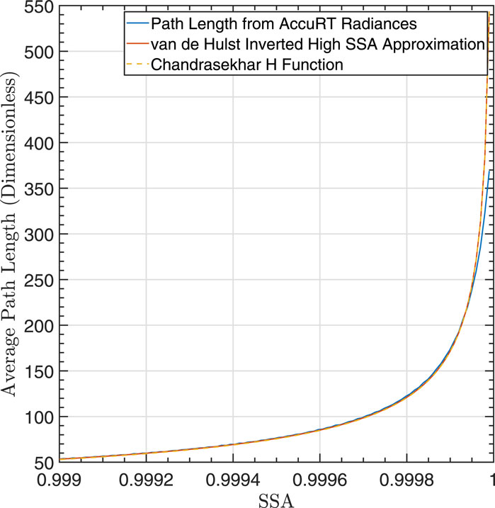
Figure 1. Comparison of the average optical path length $⟨L_{\text{opt}}⟩$ as obtained from numerical differentiation of AccuRT results (Equation 38), the van de Hulst approach (Equation 44), and the two-stream approach based on the Chandrasekhar H-function (Equation 40). AccuRT was run with a slab optical thickness ${\tau }^{*}=200$, which was sufficiently large to approximate a semi-infinite slab. We see close agreement between the results obtained from the three different methods.

4.2 Radiance reflectance ratio: two-stream vs. multi-stream results

For a semi-infinite slab consisting of a weakly absorbing matter (e.g., visible light penetration into fresh snow) the reflectance ratio $R(\varpi \le 1)/R(\varpi =1.0)$ at SSA values close to 1.0 is expected to be well approximated by the two-stream method.

For space-based lidar measurements, Hu et al. (2023) compared analytic two-stream results of the radiance ratio $R(\varpi \le 1)/R(\varpi =1)$ at SSA values close to 1.0 with results obtained via Monte Carlo simulations, and found two-stream results to agree well with accurate Monte Carlo results.

We now check if we can reproduce the results of Hu et al. (2023), but by using AccuRT computations instead of Monte Carlo simulations. Thus, we use AccuRT to obtain accurate reflectance ratios for comparison with the two-stream results. We consider SSA values in the range $0.998\le \varpi \le 1.0$ and angle cosines $\mu =1.0$, ${\mu }_0=1.0$ (mono-static lidar configuration), and $\bar{\mu }=0.6$. For these SSA and angle cosine values, we used Equation 39 to compute two-stream radiances, which were then normalized to $R(\varpi =1)$.

To compute the reflectance ratio, we used AccuRT to obtain top-of-slab radiance values for light reflected off a snow layer on the ground. We modeled the snow layer using a Henyey-Greenstein scattering phase function with asymmetry factor $g=0.0$ (isotropic scattering), and we used the same range of SSA values as Hu et al. (2023) $(0.998\le \varpi \le 1.0)$. For a fixed snow layer thickness of 1.0 m, we varied the scattering coefficients when running AccuRT to evaluate how closely the AccuRT results would compare with the analytic TSA results using ${\tau }^{*}=200$ to mimic the case of semi-infinite slab optical thickness. The radiance values were then normalized to the radiance at $\varpi =1.0$ in order to produce the radiance reflectance ratio $R(\varpi \le 1)/R(\varpi =1)$.

From Figure 2, which shows analytic two-stream results plotted against the reflectance ratio obtained via AccuRT, we see that AccuRT results corresponding to a slab optical thickness of ${\tau }^{*}=500$ agree closely with analytic TSA results. Since the TSA results are valid for a semi-infinite slab, it follows that a slab thickness of ${\tau }^{*}=500$ is sufficiently large to represent the semi-infinite case. Conversely, Figure 2 shows that AccuRT results corresponding to a slab optical thickness of ${\tau }^{*}=100$ do not agree closely with analytic TSA results. Hence, we conclude that a slab optical thickness of 100 is not sufficiently large to adequately represent a slab of semi-infinite optical thickness. The importance of the latter case is discussed further in Section 4.3.

Figure 2

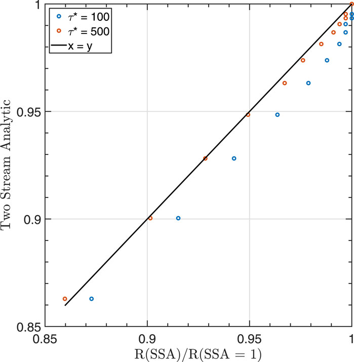
Figure 2. Comparison of normalized reflectance ratios $R(\varpi \le 1)/R(\varpi =1)$ computed by the analytic TSA method (Equation 39) (vertical axis) and by AccuRT (horizontal axis). Shown are values computed for $g=0.0$ (isotropic scattering), $\mu ={\mu }_0=1.0$, $\bar{\mu }=0.6$, and two different values of the slab optical thickness: ${\tau }^{*}=100$ and ${\tau }^{*}=500$.

4.3 How to simulate a semi-infinite case for a slab of finite physical thickness

It is important to emphasize the assumption of a semi-infinite slab when considering the results presented in Section 4.1 based on van de Hulst’s approach (Hendrik Christoffel et al., 1980). The basis of these results was the assumption of reflection from a semi-infinite slab. Thus, for a proper comparison, it is important that also AccuRT is set up to model reflection from a semi-infinite slab, which implies that all energy incident at the top of the slab must be absorbed and reflected, since, by definition, no energy can be transmitted.

For a homogenous slab of thickness $h$ and absorption and scattering coefficients $\alpha$ and $\beta$, respectively, the slab optical thickness is ${\tau }^{*}=h(\alpha +\beta )$, and the single-scattering albedo is $\varpi =\beta /(\alpha +\beta )$. In the semi-infinite limit we require ${\tau }^{*}\gg 1$. Hence, in the limit as $\varpi \to 1.0$ ($\beta \gg \alpha$), if we choose to fix the slab thickness $h$ (for example, we may use $h$ = 1.0 m for a snowpack) then we must require that $\beta \gg 1.0$.

Figure 3 demonstrates the problem that arises when AccuRT is not properly approximating the semi-infinite case. For example, if for a fixed physical slab thickness $h$, $\beta$ is not sufficiently large, the optical slab thickness ${\tau }^{*}$ will not be large enough to approximate a semi-infinite slab. In this case, some of the incident light may escape through the bottom of the slab, leading to a reduced value of the overall radiance reflected at the top of the slab. This reduced radiance value, when used in Equation 13 $[⟨L_{\text{opt}}(0,\varpi ,\infty )⟩=\frac{\partial \ln I(0,\varpi ,\infty )}{\partial \ln \varpi }]$ produces a reduced value of the average optical path length. This problem becomes quite pronounced as $\varpi \to 1.0$, as can be seen in Figure 3.

Figure 3

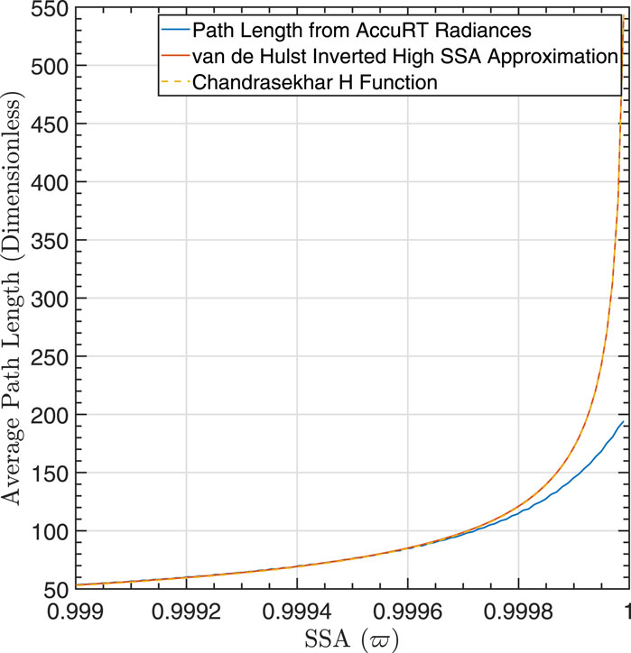
Figure 3. Comparison of the average optical path length $⟨L_{\text{opt}}⟩$ as obtained from AccuRT, the van de Hulst approach, and the two-stream approximation (TSA) based on the Chandrasekhar H-function Equation 40. In this case, AccuRT was run using a slab optical thickness that was too small to adequately approximate a semi-infinite slab. This situation leads to discrepancies between results produced by AccuRT and those produced by either the van de Hulst approximation (Equation 44) or the Chandrasekhar TSA (Equation 40) in the limit as $\varpi \to 1.0$.

A similar issue arises in the snow problem considered in Section 4.2. In this case, the relationship between the analytic TSA result for the radiance reflectance ratio and the corresponding accurate Monte Carlo result is shown to be approximately one-to-one for a slab of semi-infinite thickness. However, if the semi-infinite limit is not properly accounted for because the slab optical thickness ${\tau }^{*}$ is not chosen large enough to represent ${\tau }^{*}\to \infty$ in AccuRT, then the relationship between the analytic TSA result and the AccuRT result will no longer be represented by the one-to-one line in Figure 2. An example is shown by the blue points in Figure 2 corresponding to a slab optical thickness of ${\tau }^{*}=100$.

5 Optical path length in a slab of arbitrary optical thickness

The preceding analysis was carried out for a semi-infinite slab. From Equation 38, which represents this special case, it follows that the average optical path length depends only on one term: the derivative of the radiance with respect to the single-scattering albedo (SSA). To treat the general case of a slab of arbitrary slab optical thickness ${\tau }^{*}$, we introduce instead the “scaled” average optical path length given by (see Equation 37)

$\frac{⟨L_{\text{opt}}\left(0,\mu ,{\mu }_0,\varpi ,g,{\tau }^{*}\right)⟩}{{\tau }^{*}}=\frac{1}{{\tau }^{*}}\left[\frac{\partial \ln I_{\text{d}}^{+}}{\partial \ln \varpi }-\frac{\partial \ln I_{\text{d}}^{+}}{\partial \ln {\tau }^{*}}\right]=\frac{1}{{\tau }^{*}}\left[\frac{\varpi }{I_{\text{d}}^{+}}\frac{\partial I_{\text{d}}^{+}}{\partial \varpi }-\frac{{\tau }^{*}}{I_{\text{d}}^{+}}\frac{\partial I_{\text{d}}^{+}}{\partial {\tau }^{*}}\right](45)$

where $I_{\text{d}}^{+}\equiv I_{\text{d}}^{+}(0,\mu ,{\mu }_0,\varpi ,g,{\tau }^{*})$ is the radiance reflected from the slab. Viik (1995) presented average photon path length results for an isotropically scattering slab of finite thickness with focus on the dependence of $⟨L_{\text{opt}}⟩/{\tau }^{*}$ on the optical depth ratio, $\tau /{\tau }^{*}$. In contrast, here our interest is primarily in $⟨L_{\text{opt}}⟩/{\tau }^{*}$ values resulting due to photons reflected from the top of the slab or layer of a scattering/absorbing medium as a function of slab (or layer) IOPs and optical thickness ${\tau }^{*}$. Such results are of prime interest and importance for remote sensing applications. Here “layer” may refer to a “target layer” in lidar/radar applications (see Section 3.1).

We note that for a slab of finite optical thickness the second term in Equation 45 $[-(d{I}_{\text{d}}^{+}/d{\tau }^{*})/I_{\text{d}}^{+}]$ accounts for the change in the average path length due to the change in the slab optical thickness ${\tau }^{*}$. This term is subtracted from the first term in Equation 45, indicating that the average optical path length will be smaller for a slab of finite optical thickness than for a semi-infinite slab. We need to quantify how the second term of Equation 45 contributes to the optical path length. We expect that in the semi-infinite limit $({\tau }^{*}\to \infty )$ Equation 45 will approach Equation 38: $⟨L_{\text{opt}}(0,\mu ,{\mu }_0,\varpi ,g,\infty )⟩=\frac{\partial \ln I_{\text{d}}^{+}}{\partial \ln \varpi }=\frac{\varpi }{I_{\text{d}}^{+}}\frac{\partial I_{\text{d}}^{+}}{\partial \varpi }$. In other words, we expect that the second term of Equation 45 will approach zero as ${\tau }^{*}\to \infty$. To compute the second term, we may compute radiances at some fixed SSA value and then numerically compute the derivative of the radiance with respect to the slab optical thickness. Figure 4 shows the results of such computations, where for simplicity the radiances were computed via the analytic two-stream approximation (Equation 36) for an SSA value very close to 1.0 $(\varpi =1-10^{-9})$. From Figure 4 it is clear that the second term of Equation 43 approaches zero in the limit of a semi-infinite slab.

Figure 4

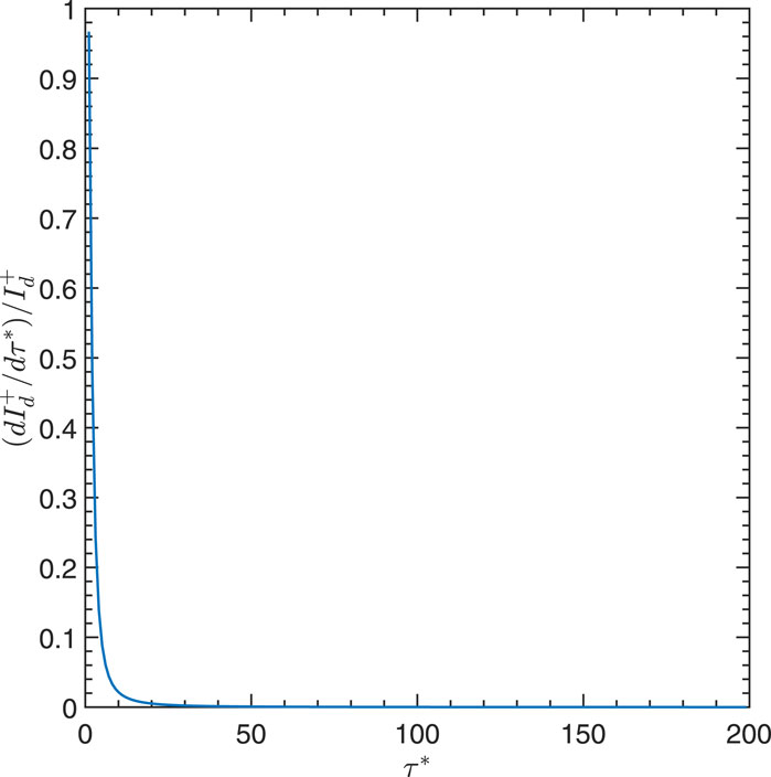
Figure 4. The derivative of upward radiance with respect to slab optical thickness (the second term of Equation 45: $(d{I}_{\text{d}}^{+}/d{\tau }^{*})/I_{\text{d}}^{+}$, as a function of the slab optical thickness. It can be seen that this derivative term approaches zero as the slab thickness increases.

We see that good results are obtained by computing the second term of Equation 45 using radiances resulting from the two-stream approximation. Thus, we may extend this approach also to the first term to provide a method for obtaining the scaled average optical path length $⟨L_{\text{opt}}⟩/{\tau }^{*}$ for a slab of arbitrary optical thickness ${\tau }^{*}$. In order to validate the results of this approach, we may compare them to those obtained by an analytical method presented by Hendrik Christoffel et al. (1980), who considered the scaled average optical path length $⟨L_{\text{opt}}⟩/{\tau }^{*}$ for a non-absorbing slab $(\varpi =1.0)$. He considered the scaled path length value in the limit of an infinitely thin slab $({\tau }^{*}\to 0)$ as well as for a semi-infinite slab $({\tau }^{*}\to \infty )$. For an infinitely thin slab, Hendrik Christoffel et al. (1980) found the scaled path length to approach the value of 1.5, and for a semi-infinite slab he found it to approach a value of 2.0.

Using the two-stream approximation, we computed radiances over a range of slab optical thicknesses from ${\tau }^{*}=0.1$ to ${\tau }^{*}=100$ at a fixed SSA value of $\varpi =1-10^{-9}$. Each term of Equation 45 was obtained via numerical differentiation. Finally, the difference between the two terms was used to obtain the scaled two-term path length, which is shown in Figure 5.

Figure 5

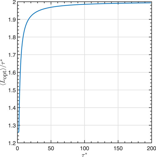
Figure 5. Scaled average optical path length (Equation 45: $\frac{⟨L_{\text{opt}}⟩}{{\tau }^{*}}=\frac{1}{{\tau }^{*}}\left[\frac{\varpi }{I_{\text{d}}^{+}}\frac{\partial I_{\text{d}}^{+}}{\partial \varpi }-\frac{{\tau }^{*}}{I_{\text{d}}^{+}}\frac{\partial I_{\text{d}}^{+}}{\partial {\tau }^{*}}\right]$) as a function of slab optical thickness ${\tau }^{*}$. Values were obtained via numerical differentiation of radiance values obtained from an analytic two-stream approximation.

Figure 5 shows that the scaled average optical path length computed using radiances obtained by the two-stream approximation approaches 2.0 in the limit of a semi-infinite slab in agreement with results reported by Hendrik Christoffel et al. (1980).

5.1 Dependence of $⟨L⟩$ on slab physical thickness $h$

It is of interest to know how the average path length of photons reflected from a slab depends on slab physical thickness $h$, since such knowledge would allow us to “translate” average path lengths into average “spans of time” spent by photons in a layer of specified physical thickness $h$. Due to multiple scattering these average “time spans” are expected to be longer than those obtained from the standard mean free path. In Figure 6A dense grid of 10,000 linearly spaced SSA values ranging from $\varpi =0.9999$ to $\varpi =1-1\times 10^{-9}$ were used to compute reflected radiances, and these computations were done for 200 linearly spaced slab physical thicknesses ranging from 0 to 20 m. Several fixed SSA values were then chosen, and the path length as a function of slab physical thickness is shown for each of these SSA values. Figure 6 shows that in the case of no absorption $(\varpi =1.0)$, there is a nearly linear relationship between the enhancement factor and the slab physical thickness. However, when even a small amount of absorptive substance is present, this linear relationship no longer holds. It can also be seen that for small slab thicknesses the relationship between the enhancement factor and the slab physical thickness is not linear. This result can be seen in both panels of Figure 6; the effect is subtle in the left panel but can be seen as a very slight upward curve as the slab physical thickness approaches zero. The effect is more plainly seen in the right panel, where the curve trends upward for slab physical thicknesses less than about 0.1 m.

Figure 6

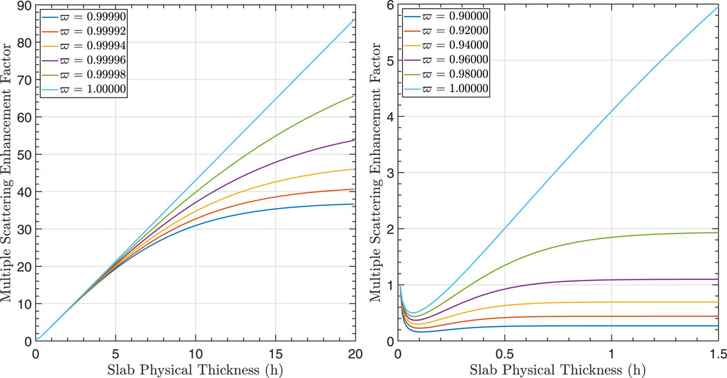
Figure 6. (A): Enhancement of the average optical path length due to multiple scattering for slab physical thickness $h$ in the range 0–20 m and SSA values in the range 0.9999–1.0. This enhancement factor is obtained by finding the average optical path length as a function of slab physical thickness $h$ [m] and then dividing by the path length in the single-scattering limit (i.e., the case of a thin slab, ${\tau }^{*}=0.01$). The average optical path length was computed via numerical differentiation of radiances obtained from the two-stream approximation. (B): Same as the left panel, but for slab physical thicknesses in the range 0–1.0 m and SSA values in the range 0.9–1.0. Note that for small slab thicknesses (i.e., less than about 0.1 m) the relationship between the enhancement factor and the slab physical thickness is not linear.

The results provided in left panel of Figure 6 might apply to a cloud of water or ice particles for which the particle density might be fixed, whereas the physical thickness might be allowed to vary. For a medium like a snowpack (or a vegetation canopy) one could fix the slab thickness (at say 1 m of snow like in the right panel of Figure 6) and vary the snow particle number density. Alternatively, for a fixed snow density, one could vary the snow pack physical thickness. In each case, one could generate results similar to those displayed in Figure 6.

5.2 Dependence of the optical path length $⟨L_{\text{opt}}⟩$ on the cosine of the beam of incidence angle

We now consider how the average optical path length depends on ${\mu }_0$, the cosine of the beam incidence angle. Following the same approach as before, we consider photons reflected in the zenith direction $(\mu =1)$, but let ${\mu }_0$ vary from near grazing incidence $({\mu }_0=0.2)$ to perpendicular incidence $({\mu }_0=1.0)$. For isotropic scattering, Figure 7 shows scaled average optical path length values as a function of slab optical thickness ${\tau }^{*}$ for photons reflected in the zenith direction $(\mu =1.0)$.

Figure 7

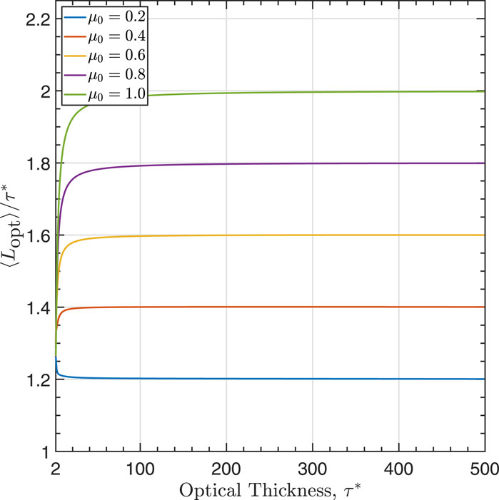
Figure 7. Scaled average optical path length (Equation 45) as a function of slab optical thickness ${\tau }^{*}$. Values were obtained via numerical differentiation of radiance values obtained from an analytic two-stream approximation. Values are shown for isotropic scattering with cosine of beam incidence angles ranging from ${\mu }_0=0.2$ to ${\mu }_0=1.0$.

Figure 7 shows that for isotropic scattering in the semi-infinite limit, the scaled optical path length approaches the value

$\frac{⟨L_{\text{opt}}\left(0,\mu ,{\mu }_0,\varpi ,g,{\tau }^{*}\right)⟩}{{\tau }^{*}}=\mu +{\mu }_0.(46)$

This result is in agreement with an analytic derivation presented by van de Hulst (Hendrik Christoffel et al., 1980), page 591.

Finally, we consider the effect of anisotropic scattering on the path length in the case of varying ${\mu }_0$. For example, Figures 8, 9 show scaled path length results at several values of ${\mu }_0$ for asymmetry factors of $g=0.5$ and $g=0.7$, respectively. Figures 8, 9 show that for a slab of finite optical thickness, the average photon path length of reflected photons is quite sensitive to the scattering phase function.

Figure 8

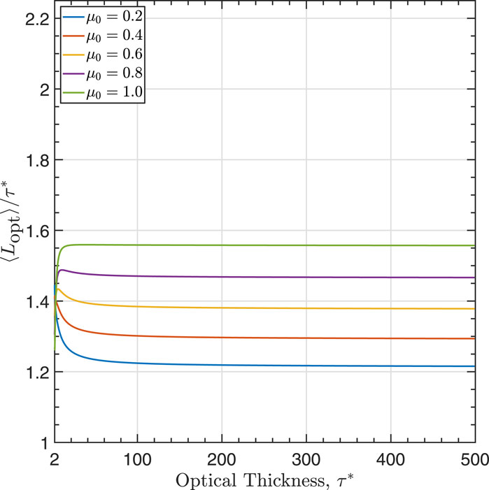
Figure 8. Scaled average optical path length (Equation 45) as a function of slab optical thickness ${\tau }^{*}$. Values were obtained via numerical differentiation of radiance values obtained from an analytic two-stream approximation. Values are shown for anisotropic scattering with $g=0.5$ and solar zenith angles ranging from ${\mu }_0=0.2$ to ${\mu }_0=1.0$.

Figure 9

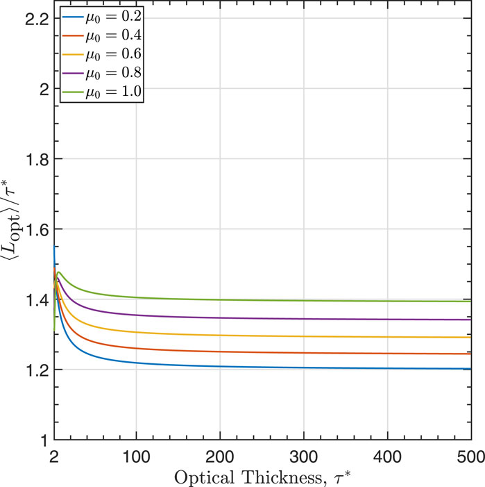
Figure 9. Scaled average optical path length (Equation 45) as a function of slab optical thickness ${\tau }^{*}$. Values were obtained via numerical differentiation of radiance values obtained from an analytic two-stream approximation. Values are shown for anisotropic scattering with $g=0.7$ and solar zenith angles ranging from ${\mu }_0=0.2$ to ${\mu }_0=1.0$.

6 Summary and conclusion

A method for determining the average photon path length due to random walks of photons in a slab consisting of multiple scattering material is presented. The method is applicable to anisotropic scattering and can be used to provide results for arbitrary slab (optical or physical) thickness. To validate the method we compare computed results with a limited number of results available in the literature, mostly for the case of a semi-infinite slab with isotropically scattering particles. The main results can be summarized as follows.

1. For isotropic scattering in an optically thick, weakly absorbing medium:

• Results produced by an analytic two-stream approximation to the radiative transfer equation (RTE) agree well with results produced by accurate multi-stream (such as discrete ordinate) solutions (see Figure 1 (average path lengths) and 2 (reflected radiances)). Both of these methods would enable one to address a variety of applications, but since the analytic two-stream solutions are computationally more efficient, they are preferred whenever they are applicable. Note that this agreement has only been demonstrated for isotropic scattering. Future work is required to determine whether the analytic two-stream method still provides good agreement with multi-stream solutions for anisotropic scattering, and if so under what conditions.

• In agreement with results reported by Hendrik Christoffel et al. (1980), for a slab of finite thickness, the average optical path length approaches 2.0 in the semi-infinite limit (see Figure 5).

• Compared to the average path length obtained in the single scattering limit the enhancement due to multiple scattering increases linearly with increase in slab physical thickness (for a fixed number density of scattering particles, see Figure 6) or with increase in particle number density for a fixed slab physical thickness) in the absence of absorption. A small amount of light absorbing material is enough to make this relationship non-linear as demonstrated in Figure 6.

$•$ Figure 7 shows scaled $⟨L_{\text{opt}}⟩/{\tau }^{*}$ results for bi-static configurations ($\mu =1.0$, ${\mu }_0$ varying). Note that in the semi-infinite limit, as $\varpi \to 1.0$ the scaled optical path length approaches the value $⟨L_{\text{opt}}(0,\mu ,{\mu }_0,\varpi ,g,{\tau }^{*})⟩/{\tau }^{*}=\mu +{\mu }_0$ in agreement with a result presented by Hendrik Christoffel et al. (1980).

2. Results for anisotropic scattering provided in Figures 8, 9 show that the average path length of photons reflected from a slab of finite optical thickness is sensitive to the anisotropy of the scattering phase function.

Finally, we should emphasize that the capability to convert average path lengths into average “time spans” spent by photons in a layer of specified physical thickness $h$ will allow us to quantify the impact of multiple scattering on the “pulse stretching” phenomenon. Thus, we may translate the results from the spatial domain into the time domain utilized by researchers in the lidar/radar community. For a medium with a constant refractive index, this transformation is straightforward. As discussed in Section 3.2, for a coupled two-slab system, such as an atmosphere overlying a body of water, the difference in refractive index between the two slabs must be considered.

Data availability statement

The raw data supporting the conclusions of this article will be made available by the authors, without undue reservation.

Author contributions

TK: Investigation, Software, Visualization, Writing – original draft, Writing – review and editing. WL: Writing – review and editing. NC: Writing – review and editing. YH: Writing – review and editing. YH: Writing – review and editing. SS: Writing – review and editing. XL: Writing – review and editing. BH: Writing – review and editing. JS: Writing – review and editing. TT: Writing – review and editing. JL: Writing – review and editing. CW: Writing – review and editing. XZ: Writing – review and editing. CG: Writing – review and editing. KS: Conceptualization, Funding acquisition, Methodology, Project administration, Supervision, Writing – original draft, Writing – review and editing.

Funding

The author(s) declare that financial support was received for the research and/or publication of this article. The authors wish to thank the NASA Remote Sensing Theory program and the NASA ESTO IIP program for supporting this research.

Conflict of interest

Authors CW and JL were employed by BAE Systems.

The remaining authors declare that the research was conducted in the absence of any commercial or financial relationships that could be construed as a potential conflict of interest.

Authors YoH, XL and TT declared that they were an editorial board member of Frontiers, at the time of submission. This had no impact on the peer review process and the final decision.

Generative AI statement

The author(s) declare that no Generative AI was used in the creation of this manuscript.

Publisher’s note

All claims expressed in this article are solely those of the authors and do not necessarily represent those of their affiliated organizations, or those of the publisher, the editors and the reviewers. Any product that may be evaluated in this article, or claim that may be made by its manufacturer, is not guaranteed or endorsed by the publisher.

Footnotes

¹In a dilute medium the concentration of particles is sufficiently low that the time between particle collisions is much longer than the duration of a collision, which implies that only binary (two-particle) collisions are important.

²If we measure altitude from the bottom of the atmosphere (slab) upwards, but optical depth from the top of the slab downwards, then for an inhomogeneous slab, we have $\tau (z)={\int }_z^{\infty }(\alpha (z^{\prime })+\beta (z^{\prime }))d{z}^{\prime }$, see Equation 15, Section 3.

³A brief note on the final step here: in Section 17.1.2, van de Hulst makes the comment that the total extinction factor has one part, $\exp \left(-L_{\text{opt}}\right)$, hidden in the factor $p(L_{\text{opt}})$. Thus we see that although the integral appears to be missing the exponential factor that would turn it into a Laplace transform, it is actually the case that this exponential factor has been subsumed into $p(L_{\text{opt}})$ and so the Laplace transform here is valid.

⁴For isotropic scattering $p_i(-\mathrm{1,1})=1\to {\mathcal{S}}_i=4\pi$.

⁵Stamnes, K., T. Kindervatter, W. Li, N. Chen,Y. Huang, Y. Hu, S. Stamnes, X. Lu, B. Hamre, T. Tanikawa, J. Lee, C. Weimer, X. Zeng, C. K. Gatebe, and J. J. Stamnes, Two-stream approximation in radiative transfer: Average Photon Path Length Estimation, Journal of the Atmospheric Sciences, accepted, 2024.

⁶The reason for using Equation 44 instead of Equation 43 is that the latter only applies to low $(\varpi \to 0)$ SSA values and thus is not applicable to the SSA values close to 1.0 used for this comparison.

References

Chandrasekhar, S. (2013). Radiative transfer. Cour. Corp.

Google Scholar

Chandrasekhar, S. (1950). Radiative Transfer. By S. Chandrasekhar. London (Oxford University Press) 1950. 8vo. Pp. 393, 35 Figures. 35 s. Quarterly Journal of the Royal Meteorological Society 76. 498–498. doi:10.1002/qj.49707633016

CrossRef Full Text | Google Scholar

Elaloufi, R., Carminati, R., and Greffet, J.-J. (2004). Diffusive-to-ballistic transition in dynamic light transmission through thin scattering slabs: a radiative transfer approach. JOSA A 21 (8), 1430–1437. doi:10.1364/josaa.21.001430

PubMed Abstract | CrossRef Full Text | Google Scholar

Hendrik Christoffel, V. de H. (1980). “Multiple light scattering: tables,” in Formulas, and applications, 2. Academic Press.

Google Scholar

Hogan, R. J. (2008). Fast lidar and radar multiple-scattering models. part i: small-angle scattering using the photon variance–covariance method. J. Atmos. Sci. 65 (12), 3621–3635. doi:10.1175/2008jas2642.1

CrossRef Full Text | Google Scholar

Hogan, R. J., and Battaglia, A. (2008). Fast lidar and radar multiple-scattering models. part ii: wide-angle scattering using the time-dependent two-stream approximation. J. Atmos. Sci. 65 (12), 3636–3651. doi:10.1175/2008jas2643.1

CrossRef Full Text | Google Scholar

Hu, Y., Lu, X., Zeng, X., Gatebe, C., Fu, Q., Yang, P., et al. (2023). Linking lidar multiple scattering profiles to snow depth and snow density: an analytical radiative transfer analysis and the implications for remote sensing of snow. Front. Remote Sens. 4. doi:10.3389/frsen.2023.1202234

CrossRef Full Text | Google Scholar

Mitra, K., and Churnside, J. H. (1999). Transient radiative transfer equation applied to oceanographic lidar. Appl. Opt. 38 (6), 889–895. doi:10.1364/ao.38.000889

PubMed Abstract | CrossRef Full Text | Google Scholar

Pierrat, R., Ben Braham, N., Rojas-Ochoa, L. F., Carminati, R., and Scheffold, F. (2008). The influence of the scattering anisotropy parameter on diffuse reflection of light. Opt. Commun. 281 (1), 18–22. doi:10.1016/j.optcom.2007.09.008

CrossRef Full Text | Google Scholar

Stamnes, K., Hamre, B., Stamnes, S., Chen, N., Fan, Y., Li, W., et al. (2018). Progress in forward-inverse modeling based on radiative transfer tools for coupled atmosphere-snow/ice-ocean systems: a review and description of the accurt model. Appl. Sci. 8 (12), 2682. doi:10.3390/app8122682

CrossRef Full Text | Google Scholar

Stamnes, K., Li, W., Stamnes, S., Hu, Y., Zhou, Y., Chen, N., et al. (2022). A novel approach to solve forward/inverse problems in remote sensing applications. Front. Remote Sens. 3, 1025447. doi:10.3389/frsen.2022.1025447

CrossRef Full Text | Google Scholar

Stamnes, K., Li, W., Stamnes, S., Hu, Y., Zhou, Y., Chen, N., et al. (2023). Laser light propagation in a turbid medium: solution including multiple scattering effects. Eur. Phys. J. D 77 (6), 110. doi:10.1140/epjd/s10053-023-00694-6

CrossRef Full Text | Google Scholar

Stamnes, K., and Stamnes, J. J. (2015). Radiative transfer in coupled environmental systems. Wiley VCH.

Google Scholar

Stamnes, K., Thomas, G. E., and Stamnes, J. J. (2017). Radiative transfer in the atmosphere and ocean. 2 edition. Cambridge University Press.

Google Scholar

Stephens, G. L., and Heidinger, A. (2000). Molecular line absorption in a scattering atmosphere. Part I: Theory. J. Atmos. Sci. 57 (10), 1599–1614. doi:10.1175/1520-0469(2000)057<1599:mlaias>2.0.co;2

CrossRef Full Text | Google Scholar

Viik, T. (1995). Average photon path-length in isotropically scattering finite atmospheres. Astrophysics Space Sci. 225, 205–219. doi:10.1007/bf00613235

CrossRef Full Text | Google Scholar