 Nathan C. Healey
 Christopher P. Barber
 Kelcy Smith1
 Jesslyn F. Brown
- 1KBR, Inc. Contractor to The U.S. Geological Survey, Earth Resources Observation and Science (EROS) Center, Sioux Falls, SD, United States
- 2U.S. Geological Survey, Earth Resources Observation and Science (EROS) Center, Sioux Falls, SD, United States
The geometric transformation of remotely sensed imagery from one map projection to another necessitates a data resampling operation which alters the recorded values. The global Landsat archive is made available in the Universal Transverse Mercator (UTM) projection system which preserves geographic shape across small area but introduces small errors in distance and area. As remote sensing-based studies develop from local scales to regional and global, they need to adopt more appropriate map projections from which accurate area measurements can be made. While effects of resampling on recorded values have been studied in the past, the impacts on higher-level results such as land cover have not been widely reported. This study investigates an approach for monitoring land cover and land change using two input datasets derived from identical source Landsat data, where one input dataset is transformed to an equal-area map projection and thereby resampled. Recorded surface reflectance values are changed through the reprojection/resampling process, and our study highlights observed differences in derived land cover from these two different input datasets throughout the various stages of deriving land cover and related characteristics. Our findings suggest that large-scale analyses of land cover will not be substantially impacted by reprojection of input data, but small-scale analyses should exercise caution when interpreting timing and magnitude of pixel-level change and classification dynamics.
1 Introduction
Applications of remote sensing have helped advance the modeling of earth surface processes and related impacts like crop yield estimation and food security, forest management practices and ecology, drought and water resource management, and carbon budgets (Wolter et al., 1995; Lark and Stafford, 1997; Jung et al., 2006; Rogan et al., 2010; Bhaga et al., 2020; Lechner et al., 2020; Karthikeyan et al., 2020). Landsat observations of Earth surface phenomena have revolutionized our understanding of Earth system science (Goward and Williams, 1997; Wulder et al., 2022). Acquiring information about land cover and associated changes to surface properties remains a fundamental motivation to sustain continuity of spaceborne observations, such as the Landsat program, into the future (Williams et al., 2006; Loveland and Dwyer, 2012; Radeloff et al., 2024). Defining best practices utilizing such a valuable archive of Earth surface observations is fundamentally important when assessments of land cover and land cover change inform decisions on how limited natural resources are managed (Brown et al., 2020). Spaceborne observations from satellites of our spherical three-dimensional Earth surface are depicted as two-dimensional images containing pixels on flat map surfaces through a broad set of transformations in the process of geospatial data projection. No matter the map projection, some level of distortion is inevitable, including when resampling a dataset into a new/different projection. Thus, methods of data handling, processing, and techniques that characterize global land change dynamics require careful consideration because something as common as reprojecting satellite data into different map projections inherently alters pixel values (Seong, 2010), especially when a dataset covers a large geographical area (Steinwand et al., 1995; Yang et al., 1996; Mulcahy, 1999; Usery, 2000; Seong and Usery, 2001; Usery and Seong, 2013). However, little is known about if and how input data resampling affects higher-order data products such as land cover. The aim of this study is to gain a better understanding of how pre-processing of Landsat input data (e.g., surface reflectance, surface temperature) potentially propagates into differences in detection of land cover and land cover change metrics. Specifically, this research investigates how Landsat input data resampling impacts output of higher-order data products of land cover classification or land cover change.
Enhanced ability to analyze atmospheric, earth surface, and subsurface properties of Earth from spaceborne sensors is undeniably beneficial for natural resource monitoring (Wulder et al., 2022). The Landsat program is currently the longest continuously acquired collection of space-based moderate-resolution land remote sensing data, beginning with the launch of the Earth Resources Technology Satellite (ERTS-1) (later renamed Landsat 1) in 1972. Land change monitoring is a well-established scientific endeavor (Anderson et al., 1976; Foody, 2002; Friedl et al., 2002; Hansen et al., 2000; Homer et al., 2004; Loveland et al., 2000; Wulder et al., 2008; Willis, 2015; Brown et al., 2020), but initial data processing steps in Landsat imagery development and management may require additional pre-processing by users depending on the application. Recognizing the importance of data management and potential issues related to resampling (or reprojection), the U.S. Geological Survey (USGS) produces two sets of Landsat data representing converted raw signals (Level-0) detected onboard Landsat spacecraft, to top-of-atmosphere (TOA) radiance (Level-1), to surface reflectance (Level-2) products: (1) U.S. Landsat Analysis Ready Data (ARD; in an Albers Equal Area Conic projection) tiled in a gridded system for the conterminous United States, Hawaii and Alaska (Earth Resources Observation and Science Center, 2021), and (2) Landsat scenes (in Universal Transverse Mercator (UTM) projection) tied to the global World Reference System-2 (i.e., Path/Row) grid which includes the global Landsat archive in its entirety (Earth Resources Observation and Science Center, 2020a; Earth Resources Observation and Science Center, 2020b; Earth Resources Observation and Science Center, 2020c; Earth Resources Observation and Science Center, 2020d).
To reduce initial steps in data processing, increase accessibility, and facilitate analysis, the USGS recognized a need for pre-packaged and pre-processed Landsat data by creating U.S. Landsat ARD (hereafter referred to as simply “ARD” for this report) for the Landsat archive from 1982-present (Dwyer et al., 2018). ARD contains data for the conterminous United States (CONUS), Alaska, and Hawaii that are tiled (5,000 × 5,000 pixel tiles or grids), georegistered, TOA radiance, and atmospherically corrected products defined in a common projection (Albers Equal Area Conic) for immediate use in monitoring and assessing landscape change (Dwyer et al., 2018). The use of ARD data has become a foundational input to large-scale (CONUS-wide) time series analyses of USGS land change science such as the Land Change Monitoring, Assessment, and Projection Initiative (LCMAP). LCMAP aimed to build a multi-decadal land cover mapping and monitoring capability for CONUS based on the strategy of utilizing every available cloud-free observation in the Landsat 30-m data record from 1982-present using a time-series analysis approach (Brown et al., 2020; Xian G. Z. et al., 2022). The ARD was developed in part to support LCMAP by providing coverage for CONUS in a single equal-area projection while minimizing projection-related data loss and simplifying data retrieval for time-series analysis (Dwyer et al., 2018).
The USGS publishes Landsat scenes from the global archive only projected in UTM. Alignment of UTM scene-based data with datasets in a different projection requires resampling. Resampling raster data via up- or down-scaling spatial resolution or simply through reprojection is common in remote sensing although users should understand the resulting impacts of reprojection and resampling on their results depending on the application, geographical extent, and phenomena being analyzed (Steinwand et al., 1995; White, 2008; Seong, 2010).
2 Materials and methods
2.1 Study site
The study region (i.e., ARD tile, hereafter referred to as the “Atlanta tile”) for this research in the southeast United States, encompassing the city of Atlanta, Georgia, was selected because it exhibits a variety of fragmented land cover types with substantial land cover change over the study period (Figure 1). Also, this region’s land use diversity has inspired previous research on urban growth (U.S. Geological Survey, 2024) and potential urban heat island impacts (Xian G. et al., 2022), highlighting the need to better understand the impacts of pixel resampling and reprojection.
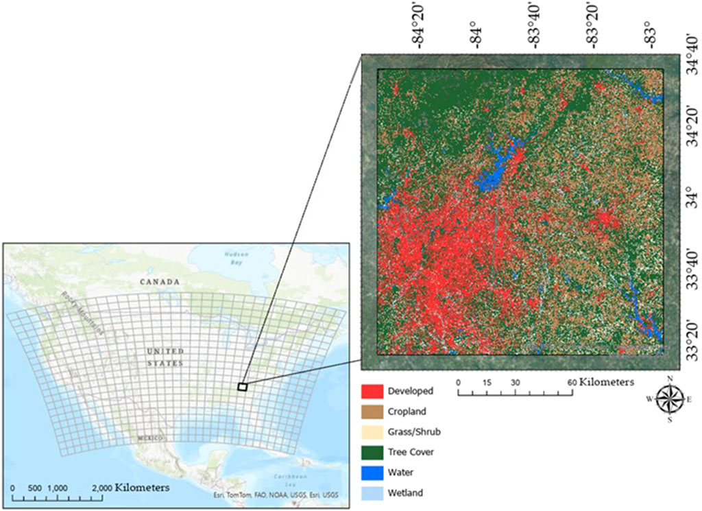
Figure 1. Study site location in this study, as defined by the U.S. Landsat Analysis Ready Data (ARD) grid, includes the Atlanta, Georgia (United States) metropolitan area, part of the Chattahoochee National Forest, various reservoirs (e.g., Lake Sydney Lanier, Lake Oconee, and Hartwell Lake), and surrounding private cropland.
2.2 Landsat data preparation
Passive optical imaging sensors onboard Landsat satellites (Landsat 5: Thematic Mapper (TM); Landsat 7: Enhanced Thematic Mapper Plus (ETM+); Landsat 8–9: Operational Land Imager (OLI)) gather photons of visible, near infrared, and shortwave infrared radiation that are spectrally dispersed to excite focal plane arrays which are translated into electrical signals (in the form of digital numbers (DNs)) leading to the formation of meaningful images or “scenes.” The process of radiometric calibration uses algorithms and processes to convert DNs (Level-0 data) for each pixel in a scene to spectral radiance (at the sensor, or TOA radiance) (Level-1 data). Geometric correction is applied to each pixel using ground control points (GCPs) and digital elevation model (DEM) data to correct for displacements caused by topographic relief. Atmospheric correction algorithms then compensate for scattering and absorption effects of the atmosphere. Once applied to TOA radiance values, a per-pixel fraction of reflected incoming solar radiation from Earth’s surface to the Landsat sensor is calculated and distributed as a Level-2 Bottom of Atmosphere (BOA) Surface Reflectance (SR) product by the USGS.
The Landsat archive has undergone a second major reprocessing effort (Collection 2) representing a culmination of improvements in absolute geolocation accuracy of the global ground reference dataset, updated global digital elevation modeling sources, and calibration and validation updates Crawford et al. (2023). Information about Collection 2 processing, geometric, and radiometric improvements can be found in a series of publications released by the USGS (Earth Resources Observation and Science Center, 2020a; Earth Resources Observation and Science Center, 2020b; Earth Resources Observation and Science Center, 2020c; Earth Resources Observation and Science Center, 2020d). For this study, two Collection 2 datasets are analyzed: (1) ARD as published by the USGS and (2) reprojected (UTM into the ARD Albers Equal Area Conic) scene-based Level-2 Landsat data using the exact same source scenes that made up the ARD data (hereafter referred to as “REP”).
Resampling of Landsat data for this study is defined as reprojecting Landsat scenes in UTM into ARD’s Albers Equal Area Conic projection using cubic convolution. Although scale distortion increases in distance away from the standard parallel, Albers Equal Area Conic is a preferred projection for land cover analyses over large areas in mid-latitude regions since it preserves relative sizes of areas across the map. To ensure consistency, spatial extents were defined by the ARD tile boundaries and the same source scenes that comprised each ARD tile were utilized in the geometric transformation from UTM to Albers Equal Area Conic. This procedure resulted in two datasets comprised of identical Landsat data in an ARD grid-defined area where one had been reprojected/resampled (REP), and one had not (ARD).
2.3 Continuous change detection and classification (CCDC)
The Continuous Change Detection (CCD) and Classification (CCDC) (Zhu and Woodcock, 2014) algorithm of time series analysis for land cover monitoring utilized in this study is specifically designed to utilize all available Level-2 Landsat surface reflectance, surface temperature, and associated quality data. CCDC is widely used in land cover studies focused on detecting land cover change pertaining to a variety of topics including forestry, agriculture, and urban development to name a few (Arevalo et al., 2020; Brown et al., 2020; Bullock et al., 2022; Friedl et al., 2022; Tang et al., 2024). Harmonic regression models characterizing the spectral response of each input band at every pixel are generated after clouds, cloud shadows, and snow are masked from all available imagery. Temporal segments of stable periods are determined by the harmonic model fits throughout the time series. Land cover change is associated with each instance where a divergence from past patterns in a temporal segment occurs, referred to as a model break. Abrupt changes leading to model breaks are often associated with phenomena like wildfires, logging practices, and surface mining operations, whereas gradual changes leading to model breaks can be associated with more slowly progressing processes like forest succession, insect infestations, or debilitating diseases. A new model is fit to each stable temporal segment of Landsat spectral observations that are separated by different model breaks. Once CCD has completed, stable segments are assigned land cover labels according to a classification algorithm paired with training data for each Landsat pixel. Land cover class definitions can be found in the Supplementary Material. For this study, we attempted to follow the data processing methodology of the USGS LCMAP program (U.S. Geological Survey, 2022) given its well documented metrics of accuracy, as well as errors and biases (Brown et al., 2020; Stehman et al., 2021). CCDC parameters and settings were taken from the LCMAP Algorithm Description Document (U.S. Geological Survey, 2022) without adjustment for specific land cover types, and the training data selection strategy also followed established protocols from LCMAP as described in Zhou et al. (2020). Here, a sample of 15.2 million randomly distributed training data pixels was generated within the ARD tile boundaries using the 2001 National Land Cover Database (NLCD) (Homer et al., 2004) aggregated to closely align with broad Anderson Land Cover Classification System Level 1 based classes (Anderson et al., 1976). Annual maps of thematic land cover for 1985–2023 were produced from CCDC using an “eXtreme Gradient Boosting” (XGBoost; Chen and Guestrin, 2016) classification model and continuous change detection (CCD) model results. All data were processed in a cloud-based environment (Amazon Web Services) via a Python-based library from the U.S. Geological Survey that implements CCDC algorithm (PyCCD; U.S. Geological Survey, 2024). CCDC has been reported previously to achieve a high level of accuracy (77.0% ± 2.0%) in North America as well as strong agreement (80%) with other global mapping endeavors like the European Space Agency (ESA) WorldCover product (Friedl et al., 2022), and the use of PyCCD in LCMAP to map eight different land cover classes has shown an accuracy of 82.5% (Stehman et al., 2021).
3 Results
3.1 Level-2 surface reflectance comparisons after resampling
As a first step, scatter plots of computed surface reflectance of the ARD and REP datasets for each Landsat band (excluding thermal infrared) were compared (Figure 2). Each scatter plot depicts the average surface reflectance values for each Landsat band, for each pixel within the Atlanta tile (25 million pixels total), for the entire study period (1985–2023). Coefficients of determination (R2) values range from 0.993 to 0.996, with Mean Absolute Differences (MAD) ranging from 0.0012 to 0.0020 and Mean Absolute Percent Differences (MAPD) ranging from 0.4% to 0.7%. The highest agreement between datasets, based on MAPD, was in the green band, and the lowest agreement was in the two shortwave infrared (SWIR1 and SWIR2) bands. Analysis of each band across the entire ARD tile indicate that the median and interquartile range percent differences are very near zero yet, a selection of outliers had differences in SR ranging from −11% to +15% (Figure 3). However, the difference between upper and lower quartiles of the 25 million pixels remains below 1%.
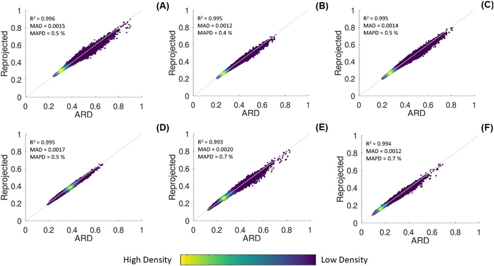
Figure 2. Comparison of average surface reflectance values from the U.S. Landsat Analysis Ready Data (ARD)-based data and the reprojected scene-based data (Universal Transverse Mercator (UTM) to ARD) for each Landsat pixel (25,000,000 pixels total) and each band (A) Blue; (B) Green; (C) Red; (D) Near Infrared; (E) Shortwave Infrared 1; (F) Shortwave Infrared 2) within the Atlanta ARD tile.
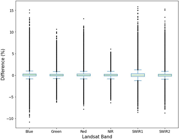
Figure 3. Box and whisker plots of average scene-wide differences (%) in surface reflectance values for each Landsat band in the Atlanta tile. Each data point represents a single pixel’s average value from 1985 to 2023.
3.2 CCDC comparisons after resampling
After comparison of surface reflectance values, each dataset was processed through the CCD algorithm. Figure 4 shows how slight differences in surface reflectance propagate into differences in the number of model breaks generated. However, the difference of annual total number of model breaks for all pixels within the Atlanta tile remains small with an R2 value of 0.9989, MAD of 17,314, and MAPD of only 3%. Across the Atlanta tile, the annual total number of model breaks generated by CCD is similar between the ARD and REP datasets (Figure 4), and the distribution of model break abundance for the entire timeseries follows similar patterns spatially (Figures 5A,B). Of the 25 million pixels in the tile, most experience either no breaks (i.e., no land cover change from 1985 to 2023), or as few as two breaks. Some areas of the Atlanta tile showed heightened model break abundance. Most of these areas had three to eight model breaks, with some pixels experiencing a maximum of 18 total model breaks throughout the time series. An example of a location experiencing heightened abundance of model breaks is highlighted in Figures 5C–E.
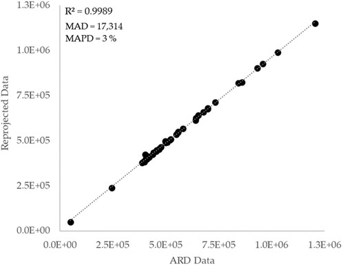
Figure 4. Annual number of model breaks from U.S. Landsat Analysis Ready Data (ARD) and for scene-based data (i.e., reprojected from Universal Transverse Mercator (UTM) to ARD using the exact same scenes that were used in the creation of the ARD data) for the Atlanta tile from 1985 to 2023 derived from the Continuous Change Detection and Classification (CCDC) algorithm.
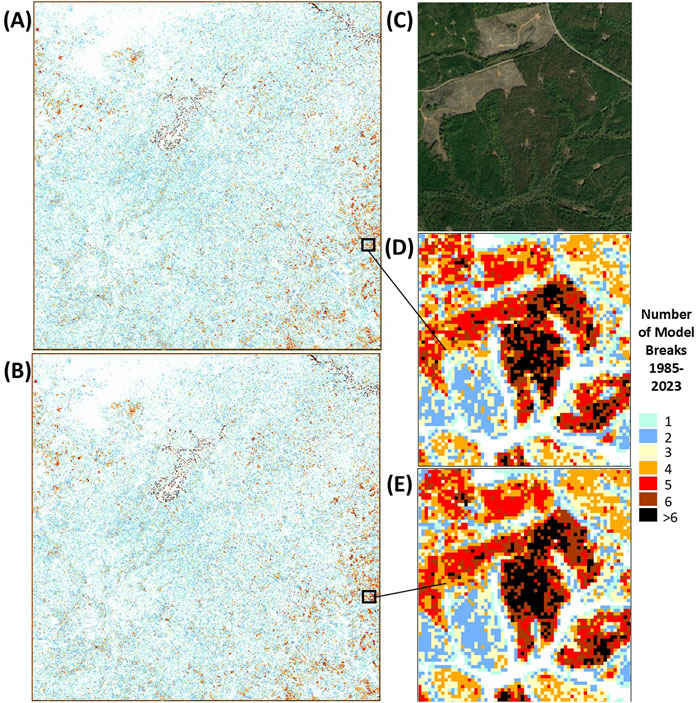
Figure 5. Annual number of model breaks from U.S. Landsat Analysis Ready Data (ARD) (A) and for reprojected scene-based data (REP) (B) for the Atlanta ARD tile region from 1985 to 2023 derived from the Continuous Change Detection and Classification (CCDC) algorithm. A true color image (C) of a location showing some of the highest number of model breaks in this region is shown with detailed depictions of the differences between the ARD (D) and REP (E) outputs at a location experiencing rotational timber harvest in north central Georgia, USA.
3.3 Classification comparisons after resampling
Pixel values in land cover categories resulting from the CCDC algorithm following class definitions outlined by the USGS LCMAP program (U.S. Geological Survey, 2020) show close agreement between the ARD and REP input datasets. The highest agreement of land cover classification between the two datasets was for pixels being classified as Tree Cover, followed by Developed, and Cropland (Figure 6). Barren land and Water had the next highest agreement. The greatest disagreements were when processing of one dataset resulted in pixels classified as Tree Cover and the other resulted in a classification of either Developed or Barren classes.
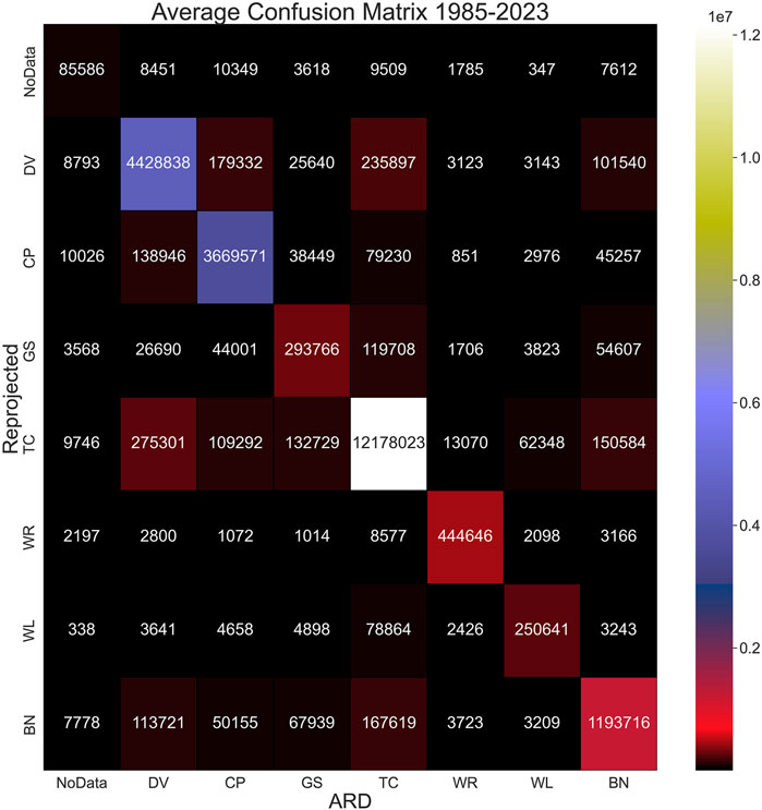
Figure 6. Average confusion matrix for classifications derived using the Continuous Change Detection and Classification (CCDC) algorithm for the Atlanta tile representing classifications of all 25 million pixels per year from 1985 to 2023. Land cover class abbreviations: TC = Tree Cover, DV = Developed, CP = Cropland, GS = Grass/Shrub, WL = Wetland, WR = Water, BN = Barren, No Data = no classification derived from CCDC.
Overall, tile-level annual land cover composition resulted in similar outputs between the ARD and REP datasets (Figure 7). Land cover trajectories were closely mimicked by both datasets through time, and both show that Tree Cover, Developed, and Cropland are the three classes covering the largest area of the Atlanta tile, respectively (Figure 7, also refer to Supplementary Material). Both datasets show increases in Developed land, Grass/Shrub, Cropland, and Water throughout the time series. Results show a decrease in Barren, Tree Cover, and Wetland classes (Table 1). Interannual variations in land cover composition, and computed differences between the outputs (ARD vs. REP), are shown in greater detail in the Supplementary Material. These Supplementary plots show a steady increase in Developed land and substantial decreases in Water. Differences between ARD and REP composition are quite small with R2, MAD, and MAPD values ranging from 0.923 to 0.999, 5–75 km2, and 0.5%–5.7%, respectively (refer to Supplementary Material).
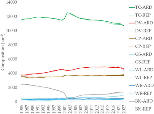
Figure 7. Annual Atlanta tile land cover composition for the U.S. Landsat ARD-based data (ARD) and scene-based (i.e., reprojected) data (REP) for 1985 to 2023 (Land cover class abbreviations: TC = Tree Cover, DV = Developed, CP = Cropland, GS = Grass/Shrub, WL = Wetland, WR = Water, BN = Barren). Plots of individual land cover classes are available in the Supplementary Material.
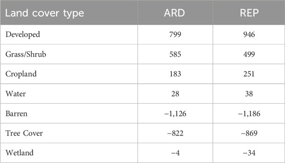
Table 1. Differences in area (km2) of each land cover type for the reprojected scene-based dataset (REP) and the U.S. Landsat ARD-based dataset (ARD) calculated by subtracting the 2023 value from the 1985 value.
Differences in annual classifications are noticeable in years surrounding periods of land cover change. Figure 8 shows an example of a pixel from the region in Figure 5 that experienced heightened model breaks. The associated land cover classification of the CCDC outputs resulting from the ARD and REP input datasets are similar yet clearly not identical. This example shows a forested location that is harvested in the late 1990s, followed by a regeneration period, and then the location is harvested again in the middle 2010s.
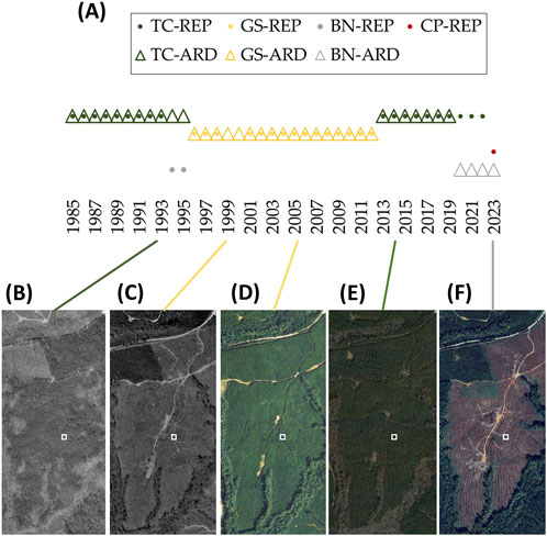
Figure 8. Output for an example pixel (−83.1244 W, 33.6830 N) of annual land cover composition using the U.S. Landsat ARD-based data (ARD) and reprojected scene-based data (REP) for 1985 to 2023 (A). Location of the example pixel is identified by a box in (B–F). (Land cover class abbreviations: TC = Tree Cover, GS = Grass/Shrub, BN = Barren, CP = Cropland).
4 Discussion
Anytime remotely sensed data are resampled or reprojected, an unavoidable transformation occurs that alters the original pixel values. In this study, Landsat Collection 2 UTM data are reprojected into the ARD Albers Equal Area Conic projection using cubic convolution as provided by the Rasterio python library (Gillies et al., 2013), where the new value of each pixel is calculated by fitting a smooth curve based on the surrounding pixels. While other resampling methods exist, cubic convolution is generally accepted to be most appropriate for use when reprojecting continuous field satellite imagery and is the method used by the USGS when producing Landsat products (Earth Resources Observation and Science Center, 2020a; Earth Resources Observation and Science Center, 2020b; Earth Resources Observation and Science Center, 2020c; Earth Resources Observation and Science Center, 2020d). When raster data are reprojected using calculations within a geometric transformation model, images are warped from the original projection space (here: UTM) to the desired projection space (here: ARD Albers Equal Area Conic). This is well established in remote sensing, although the impacts of such transformations in higher levels of data processing are less well understood, hence the motivation for this study. The resulting reprojected pixel values are similar although this research demonstrates that they are clearly not the same. Previous research by Steinwand et al. (1995) indicates that a potential reason for the difference in pixel values between datasets in this study being so small is related to a limited amount of geometric distortion when reprojecting from UTM to a conical projection for the southeastern United States. Changes to pixel values are expected during reprojection, but the degree to which changes in surface reflectance impacts local and regional scale features produced in subsequent data processing such as classification of land cover was unreported prior to this study. The results of this study indicate that small changes in surface reflectance due to reprojection have fine-scale impacts on input data but do not significantly alter land cover classification or detection of changes in land cover in large-scale analyses.
Differences in change detection produced by CCDC after input data reprojection are subtly important, depending on the scale of the application of land cover outputs. Large-scale metrics from this study indicate that the change is quite small (MAPD = 3%) when anywhere from ∼50,000 to 1,200,000 model breaks occur annually across the entire Atlanta tile. Small-scale investigations into the results from this study indicate that the abundance and timing of CCDC model breaks can vary depending on the input dataset. Previous studies without input data reprojection have noted similar difficulty in detection of small-scale land cover change timing as well as classification confusion. For example, classification labeling uncertainty for early successional forest has been confused with cropland, and recently logged areas with little detectable vegetation can lead to classifications of grassland or bare soil (i.e., Barren) (Kinnebrew et al., 2022). Small-scale, gradual spatiotemporal changes, like insect infestations in forests, are challenging to quantify (Pouliot et al., 2014; He et al., 2024). Nevertheless, small differences in the abundance and timing of model breaks does not significantly impact delineation of landscape features (forests, urban areas, etc.) or changes at larger (i.e., ARD tile-level) scales. Applications focused on small-scale geospatial changes (pixel-level) to land cover will notice that resampling pixels can have a greater influence on results than applications focused on more large-scale (ARD tile-level) analyses of land cover dynamics. Areas where there are three or more breaks commonly represent areas experiencing natural (e.g., water-level fluctuations in a lake/reservoir or drought impacts on national forests) or anthropogenic influences (e.g., forestry, mining, or urbanization) on land cover dynamics. For instance, interannual water level rise and fall along shorelines of lakes/reservoirs increases model break potential (i.e., land cover change), and areas where commercial timber production is occurring inherently experience greater probability of model breaks occurring. In the context of this example, finer-scale analyses of lake surface area or small-scale tree stand monitoring will vary, depending on whether the input data have been resampled. In a larger, more landscape-scale context, the fluctuation of model breaks and resulting land cover classes on a proportionally small number of pixels relative to the entire tile comprised of 25 million pixels, will be less impactful on overall landscape-level analyses of land cover change through time, regardless of whether the data were resampled or not. Our results show that both ARD and REP datasets show similar large-scale change abundance and timing.
For this particular region, our results indicate that analyses focused on large- or regional-scale Tree Cover, Developed, and Cropland compositional dynamics would likely obtain similar results in terms of CCDC outputs of change detection and classification/composition after input data are reprojected. However, discrepancies in classification associated with all other classes begin to increase after input data have been reprojected and run through the CCDC algorithm. We highlight a fine-scale example of a location experiencing commercial timber production where land cover classification and model breaks (i.e., land cover change) through the time series are quite similar, but some important distinctions are revealed. For example, the timing of Tree Cover removal (i.e., timber harvest) is captured by both sets of results, but the REP data output classified the pixel as Barren for 2 years prior to becoming Grass/Shrub whereas the ARD remained tree cover and switched abruptly to Grass/Shrub. Both datasets captured the transition timing from Grass/Shrub to Tree Cover in the same year, but when the plot was harvested a second time, the ARD data converted to Barren for the final 4 years of the time series whereas the REP data remained Tree Cover for three of the last 4 years before converting to Cropland. Clearly, this location is not used as Cropland, but the final year of the time series of the REP data resulted in an unrealistic classification. This artifact of reprojection could be very important if research is focused on very fine geographic scales or plot-level dynamics. If natural resource managers are relying on land cover mapping using CCDC for assessment of large-scale compositional changes through time, reprojection will not likely invalidate such an approach. However, reprojection is shown to alter the time series of events related to timing of model breaks (i.e., land cover change) and resulting classification, so caution should be exercised if a reprojection of the input data occurs.
Limitations to this study include the fact that only one ARD tile has been investigated. However, with 25 million pixels to survey over a study period of 38 years, we consider this sample size to be adequate for this study. Future research could investigate a variety of ARD tiles representing a diverse spectrum of biogeographical conditions that have been impacted by land cover change in different ways. The land cover classes in this study are intentionally broad in their definitions, which could be adjusted in future work to understand how resampling of input data may impact more specific land cover classes (e.g., Tree Cover versus Deciduous/Evergreen Trees). We also only considered the geometric transformation and associated resampling of imagery from UTM to an Albers Equal Area Conic projection. We expect that other land cover monitoring applications would apply a similar equal area conic projection (e.g., Lambert) if UTM was unsatisfactory and that the impact of transformation and resampling would be similar. Applications where impacts of input data resampling need to be rigorously quantified may seek to repeat investigations we have demonstrated here for applications-specific projections, geographies, and/or output data types.
In conclusion, the observed time-series models and resulting land cover outputs from REP data are not significantly different from ARD inputs on larger scales. Surface reflectance values change during the resampling procedures in reprojection of raster data pixels, and these differences propagate through the CCDC algorithm by producing varying levels of change detection model breaks and varying land cover classification of interannual pixel values. The scale of applications is important when considering the impacts of input data reprojection. On small spatial scales (i.e., pixel to plot level) differences in model breaks and land cover classification could complicate interannual analyses on land cover dynamics. On larger spatial scales (regional to tile-wide), the differences introduced by input data reprojection are relatively small. In summary, caution should be exercised when interpreting the results of algorithmic outputs of land cover change and composition, depending on the scale of the analysis and research goals.
Data availability statement
Details and sources of Collection 2 Landsat data archive (Level-1, Level-2, and Level-3 data products) can be found at https://www.usgs.gov/landsat-missions/landsat-data-access. A variety of sources provide access to the Landsat data archives including the USGS EarthExplorer (https://earthexplorer.usgs.gov), commercial cloud access (https://www.usgs.gov/landsat-missions/landsat-commercial-cloud-data-access), GloVis (https://glovis.usgs.gov), Landsat Look (https://landsatlook.usgs.gov), the USGS Earth Observation and Science (EROS) Center Science Processing Architecture (ESPA) On-Demand interface (https://espa.cr.usgs.gov), and NASA AppEEARS portal (https://appeears.earthdatacloud.nasa.gov). The Albers scenes that go into ARD tiling are published via Amazon Web Services (AWS) S3, and the USGS Landsat data can be accessed using the USGS SpatioTemporal Asset Catalog (STAC) at https://www.usgs.gov/landsat-missions/spatiotemporal-asset-catalog-stac.
Author contributions
NH: Conceptualization, Data curation, Formal Analysis, Investigation, Methodology, Writing – original draft, Writing – review and editing. CB: Conceptualization, Funding acquisition, Investigation, Methodology, Project administration, Supervision, Writing – review and editing. KS: Conceptualization, Data curation, Investigation, Methodology, Software, Writing – review and editing. RM: Data curation, Investigation, Methodology, Software, Writing – review and editing. JB: Conceptualization, Funding acquisition, Project administration, Writing – review and editing. CR: Data curation, Investigation, Methodology, Writing – review and editing.
Funding
The author(s) declare that financial support was received for the research and/or publication of this article. This work was supported by the U.S. Geological Survey under contract 140G0121D0001.
Acknowledgments
We thank our colleagues at the USGS EROS Center for feedback on manuscript preparation and analysis strategies, and our peer reviewers from the journal. Any use of trade, firm, or product names is for descriptive purposes only and does not imply endorsement by the U.S. Government.
Conflict of interest
Authors NH, KS, RM, and CR were employed by KBR, Inc.
The remaining authors declare that the research was conducted in the absence of any commercial or financial relationships that could be construed as a potential conflict of interest.
Generative AI statement
The author(s) declare that no Generative AI was used in the creation of this manuscript.
Publisher’s note
All claims expressed in this article are solely those of the authors and do not necessarily represent those of their affiliated organizations, or those of the publisher, the editors and the reviewers. Any product that may be evaluated in this article, or claim that may be made by its manufacturer, is not guaranteed or endorsed by the publisher.
Supplementary material
The Supplementary Material for this article can be found online at: https://www.frontiersin.org/articles/10.3389/frsen.2025.1570580/full#supplementary-material
References
Anderson, J. R., Hardy, E. E., Roach, J. T., and Witmer, R. E. (1976). A land use and land cover classification system for use with remote sensor data, 964. Washington, DC: US Government Printing Office. doi:10.3133/pp964
Arevalo, P., Bullock, E. L., Woodcock, C. E., and Olofsson, P. (2020). A suite of tools for continuous land change monitoring in Google Earth Engine. Front. Clim. 2, 576740. doi:10.3389/fclim.2020.576740
Bhaga, T. D., Dube, T., Shekede, M. D., and Shoko, C. (2020). Impacts of climate variability and drought on surface water resources in sub-Saharan Africa using remote sensing: a review. Rem. Sens. 12 (24), 4184. doi:10.3390/rs12244184
Brown, J. F., Tollerud, H. J., Barber, C. P., Zhou, Q., Dwyer, J. L., Vogelman, J. E., et al. (2020). Lessons learned implementing an operational continuous United States national land change monitoring capability: the Land Change Monitoring, Assessment, and Projection (LCMAP) approach. Rem. Sens. Environ. 238, 111356. doi:10.1016/j.rse.2019.111356
Bullock, E. L., Healey, S. P., Yang, Z., Houborg, R., Gorelick, N., Tang, X., et al. (2022). Timeliness in forest change monitoring: a new assessment framework demonstrated using Sentinel-1 and a continuous change detection algorithm. Rem. Sens. Environ. 276, 113043. doi:10.1016/j.rse.2022.113043
Chen, T., and Guestrin, C. (2016). “XGBoost: a scalable tree boosting system,” in Kdd '16: proceedings of the 22nd ACM SIGKDD international conference on knowledge discovery and data mining, 785–794. doi:10.1145/2939672.2939785
Crawford, C. J., Roy, D. P., Arab, S., Barnes, C., Vermote, E., Hulley, G., et al. (2023). The 50-year Landsat collection 2 archive. Sci. Remote. Sens. 8, 100103. doi:10.1016/j.srs.2023.100103
Dwyer, J. L., Roy, D. P., Sauer, B., Jenkerson, C. B., Zhang, H., and Lymburner, L. (2018). Analysis ready data—enabling analysis of the Landsat archive. Rem. Sens. 10 (9), 1363. doi:10.3390/rs10091363
Earth Resources Observation and Science (EROS) Center (2020d). Landsat 1-5 multispectral scanner level-1, collection 2. U.S. Geol. Surv. doi:10.5066/P9AF14YV
Earth Resources Observation and Science (EROS) Center (2020c). Landsat 4-5 thematic mapper level-1, collection 2. U.S. Geol. Surv. doi:10.5066/P918ROHC
Earth Resources Observation and Science (EROS) Center (2020b). Landsat 7 enhanced thematic mapper Plus level-1, collection 2. U.S. Geol. Surv. doi:10.5066/P9TU80IG
Earth Resources Observation and Science (EROS) Center (2020a). Landsat 8-9 operational land imager/thermal infrared sensor level-1, collection 2. U.S. Geol. Surv. doi:10.5066/P975CC9B
Earth Resources Observation and Science (EROS) Center (2021). Landsat 4-9 U.S. Analysis ready data, collection 2. U.S. Geol. Surv. doi:10.5066/P960F8OC
Foody, G. M. (2002). Status of land cover classification accuracy assessment. Rem. Sens. Environ. 80 (1), 185–201. doi:10.1016/S0034-4257(01)00295-4
Friedl, M. A., McIver, D. K., Hodges, J. C. F., Zhang, X. Y., Muchoney, D., Strahler, A. H., et al. (2002). Global land cover mapping from MODIS: algorithms and early results. Rem. Sens. Environ. 83 (1), 287–302. doi:10.1016/S0034-4257(02)00078-0
Friedl, M. A., Woodcock, C. E., Olofsson, P., Zhu, Z., Loveland, T., Stanimirova, R., et al. (2022). Medium spatial resolution mapping of global land cover and land cover change across multiple decades from Landsat. Front. Rem. Sens. 3, 894571. doi:10.3389/frsen.2022.894571
Gillies, S., Steward, A. J., Snow, A. D., Culquicondor, A., Amici, A., Shepard, A., et al. (2013). Rasterio: geospatial raster I/O for Python programmers. Mapbox. Available online at: https://github.com/rasterio/rasterio.
Goward, S. N., and Williams, D. L. (1997). Landsat and earth systems science: development of terrestrial monitoring. Photogram. Eng. Rem. Sens. 63 (7), 887–900.
Hansen, M. C., Defries, R. S., Townshend, J. R. G., and Sohlberg, R. (2000). Global land cover classification at 1 km spatial resolution using a classification tree approach. Int. J. Rem. Sens. 21 (6-7), 1331–1364. doi:10.1080/014311600210209
He, H., Yan, J., Liang, D., Sun, Z., Li, J., and Wang, L. (2024). Time-series land cover change detection using deep learning-based temporal semantic segmentation. Rem. Sens. Environ. 305, 114101. doi:10.1016/j.rse.2024.114101
Homer, C., Huang, C., Yang, L., Wylie, B., and Coan, M. (2004). Development of a 2001 national land-cover database for the United States. Photogram. Eng. Rem. Sens. 70 (7), 829–840. doi:10.14358/PERS.70.7.829
Jung, M., Henkel, K., Herold, M., and Churkina, G. (2006). Exploiting synergies of global land cover products for carbon cycle modeling. Rem. Sens. Environ. 101 (4), 534–553. doi:10.1016/j.rse.2006.01.020
Karthikeyan, L., Chawla, I., and Mishra, A. K. (2020). A review of remote sensing applications in agriculture for food security: crop growth and yield, irrigation, and crop losses. J. Hydrol. 586, 124905. doi:10.1016/j.jhydrol.2020.124905
Kinnebrew, E., Ochoa-Brito, J. I., French, M., Millis-Novoa, M., Shoffner, E., and Siegel, K. (2022). Biases and limitations of Global Forest Change and author-generated land cover maps in detecting deforestation in the Amazon. PLoS ONE 17 (7), e0268970. doi:10.1371/journal.pone.0268970
Lark, R. M., and Stafford, J. V. (1997). Classification as a first step in the interpretation of temporal and spatial variation of crop yield. Ann. App. Biol. 130, 111–121. doi:10.1111/j.1744-7348.1997.tb05787.x
Lechner, A. M., Foody, G. M., and Boyd, D. S. (2020). Applications in remote sensing to forest ecology and management. One Earth 2, 405–412. doi:10.1016/j.oneear.2020.05.001
Loveland, T. R., and Dwyer, J. L. (2012). Landsat: building a strong future. Rem. Sens. Environ. 122, 22–29. doi:10.1016/j.rse.2011.09.022
Loveland, T. R., Reed, B. C., Brown, J. F., Ohlen, D. O., Zhu, Z., Yang, L., et al. (2000). Development of a global land cover characteristics database and IGBP DISCover from 1 km AVHRR data. Int. J. Rem. Sens. 21 (6–7), 1303–1330. doi:10.1080/014311600210191
Mulcahy, K. A. (1999). Spatial data sets and map projections: an analysis of distortion. Phd Dissertation. New York, NY: Graduate School and University Center, City University of New York. DAI-A 60/01.
Pouliot, D., Latifovic, R., Zabcic, N., Guindon, L., and Olthof, I. (2014). Development and assessment of a 250 m spatial resolution MODIS annual land cover time series (2000–2011) for the forest region of Canada derived from change-based updating. Rem. Sens. Environ. 140, 731–743. doi:10.1016/j.rse.2013.10.004
Radeloff, V. C., Roy, D. P., Wulder, M. A., Anderson, M., Cook, B., Crawford, C. J., et al. (2024). Need and vision for global medium-resolution Landsat and Sentinel-2 data products. Rem. Sens. Environ. 300, 113918. doi:10.1016/j.rse.2023.113918
Rogan, J., Bumbarger, N., Kulakowski, D., Christman, Z. J., Runfola, D. M., and Blanchard, S. D. (2010). Improving forest type discrimination with mixed life-form classes using fuzzy classification thresholds informed by field observations. Can. J. Rem. Sens. 36, 699–708. doi:10.5589/m11-009
Seong, J. C. (2010). Modelling the accuracy of image data reprojection. Int. J. Rem. Sens. 24 (11), 2309–2321.
Seong, J. C., and Usery, E. L. (2001). Modeling the raster representation accuracy using a scale factor model. Photogram. Eng. Rem. Sens. 67, 1185–1191. doi:10.1080/01431160210154038
Stehman, S. V., Pengra, B., Horton, J., and Wellington, D. F. (2021). Validation of the U.S. Geological survey’s land change monitoring, assessment and projection (LCMAP) collection 1.0 annual land cover products 1985–2017. Rem. Sens. Environ. 265, 112646. doi:10.1016/j.rse.2021.112646
Steinwand, D. R., Hutchinson, J. A., and Snyder, J. P. (1995). Map projections for global and continental data sets and an analysis of pixel distortion caused by reprojection. Photogram. Eng. Rem. Sens. 61, 1487–1497.
Tang, X., Barrett, M. G., Cho, K., Bratley, K. H., Tarrio, K., Zhang, Y., et al. (2024). Broad-area-search of new construction using time series analysis of Landsat and Sentinel-2 data. Sci. Rem. Sens. 9, 100138. doi:10.1016/j.srs.2024.100138
Usery, E. L. (2000). MAUP: modifiable Areal Unit Problem in raster GIS datasets. Raster pixels as modifiable areas. GIM Int. 15 (8), 43–45.
Usery, E. L., and Seong, J. C. (2013). All equal-area map projections are created equal, but some equal-area map projections are more equal than others. Cartogr. Geogr. Info. Syst. 28, 183–193. doi:10.1559/152304001782153053
U.S. Geological Survey (USGS) (2020). Land change monitoring, assessment, and projection (LCMAP) data Format control Book (DFCB). U.S. Geol. Surv. LSDS 1424. Available online at: https://www.usgs.gov/media/files/lcmap-dfcb.
U.S. Geological Survey (USGS) (2022). Land change monitoring, assessment, and projection (LCMAP) collection 1.3 continuous change detection and classification (CCDC) algorithm description document (ADD). LSDS-2345, version 1.0. Available online at: https://www.usgs.gov/media/files/lcmap-collection-13-ccdc-add.
White, D. (2008). Display of pixel loss and replication in reprojecting raster data from the sinusoidal projection. Geocarto Int. 21 (2), 19–22. doi:10.1080/10106040608542379
Williams, D. L., Goward, S., and Arvidson, T. (2006). Landsat: yesterday, today, and tomorrow. Photogram. Eng. Rem. Sens. 72 (10), 1171–1178. doi:10.14358/PERS.72.10.1171
Willis, K. S. (2015). Remote sensing change detection for ecological monitoring in United States protected areas. Biol. Conserv. 182, 233–242. doi:10.1016/j.biocon.2014.12.006
Wolter, P. T., Mladenoff, D. J., Host, G. E., and Crow, T. R. (1995). Improved forest classification in the northern Lake State using multi-temporal Landsat imagery. Photogram. Eng. Rem. Sens. 61 (9), 1129–1143.
Wulder, M. A., Roy, D. P., Radeloff, V. C., Loveland, T. R., Anderson, M. C., Johnson, D. M., et al. (2022). Fifty years of Landsat science and impacts. Rem. Sens. Environ. 280, 113195. doi:10.1016/j.rse.2022.113195
Wulder, M. A., White, J. C., Goward, S. N., Masek, J. G., Irons, J. R., Herold, M., et al. (2008). Landsat continuity: issues and opportunities for land cover monitoring. Rem. Sens. Environ. 112 (3), 955–969. doi:10.1016/j.rse.2007.07.004
Xian, G., Shi, H., Zhou, Q., Auch, R., Gallo, K., Wu, Z., et al. (2022b). Monitoring and characterizing multi-decadal variations of urban thermal condition using time-series thermal remote sensing and dynamic land cover data. Rem. Sens. Environ. 269, 112803. doi:10.1016/j.rse.2021.112803
Xian, G. Z., Smith, K., Wellington, D., Horton, J., Zhou, Q., Li, C., et al. (2022a). Implementation of the CCDC algorithm to produce the LCMAP Collection 1.0 annual land surface change product. Earth Syst. Sci. Data 14 (1), 143–162. doi:10.5194/essd-14-143-2022
Yang, L., Zhu, Z., Izaurralde, J., and Merchant, J. (1996). Evaluation of North and South America AVHRR 1-km data for global environmental modeling, 21–26 January1996. Santa Fe, New Mexico, USA: NCGIA Third International Conference/Workshop on Integrating GIS and Environmental Modeling.
Zhou, Q., Tollerud, H., Barber, C., Smith, K., and Zelenak, D. (2020). Training data selection for annual land cover classification for the land change monitoring, assessment, and projection (LCMAP) initiative. Rem. Sens. 12 (4), 699. doi:10.3390/rs12040699
Keywords: land cover, reprojection, resampling, classification, land cover change
Citation: Healey NC, Barber CP, Smith K, Mital R, Brown JF and Robison C (2025) Resiliency of land change monitoring efforts to input data resampling. Front. Remote Sens. 6:1570580. doi: 10.3389/frsen.2025.1570580
Received: 03 February 2025; Accepted: 08 May 2025;
Published: 06 June 2025.
Edited by:
Cláudia Maria Almeida, National Institute of Space Research (INPE), BrazilReviewed by:
Antonio Fonseca, Clark University, United StatesXiaofeng Lin, Jimei University, China
Rodrigo Macedo, Federal University of Paraná, Brazil
Copyright At least a portion of this work is authored by Christopher P. Barber and Jesslyn F. Brown on behalf of the U.S. Government and as regards Dr. Barber, Ms. Brown and the U.S. Government, is not subject to copyright protection in the United States. Foreign and other copyrights may apply. This is an open-access article distributed under the terms of the Creative Commons Attribution License (CC BY). The use, distribution or reproduction in other forums is permitted, provided the original author(s) or copyright owner(s) are credited and that the original publication in this journal is cited, in accordance with accepted academic practice. No use, distribution or reproduction is permitted which does not comply with these terms.
*Correspondence: Nathan C. Healey, bmhlYWxleUBjb250cmFjdG9yLnVzZ3MuZ292