 Harald Zandler1*
 Jakob Abermann1
 Benjamin A. Robson2
 Alexander Maschler3Thomas Scheiber3
 Jonathan L. Carrivick4
 Jacob C. Yde3
- 1Department of Geography and Regional Science, University of Graz, Graz, Austria
- 2Department of Earth Science, University of Bergen, Bergen, Norway
- 3Department of Civil Engineering and Environmental Sciences, Western Norway University of Applied Sciences, Sogndal, Norway
- 4School of Geography and Water@leeds, University of Leeds, Leeds, United Kingdom
Remote sensing is a key tool to derive glacier surface velocities but existing mapping methods, such as cross-correlation techniques, can fail where surface properties change temporally or where large velocity variations occur spatially. High-resolution datasets, such as UAV imagery, offer a promising solution to tackle these issues and to study small-scale glacier dynamics, but new workflows are required to handle such data. Therefore, we tested the potential of new deep learning-based image-matching algorithms for deriving glacier surface velocities across the ablation area of a glacier with strong spatial variability in surface velocities (<5 m/yr to >100 m/yr) and substantial changes in surface properties between image acquisitions. For a thorough comparison of state-of-the-art methods and sensors, we applied three different techniques (cross-correlation using geoCosiCorr3D, feature tracking with ORB using SeaIceDrift and the new deep learning-based method using ICEpy4D) and three different platforms (Sentinel-2, PlanetScope, UAVs) to estimate glacier surface velocities. Results showed lowest errors for velocities derived with the deep learning-based approach applied to UAV imagery (RMSE = 2.17 m/yr, R2 = 0.99), followed by cross-correlation using Sentinel-2 images (RMSE = 21.0 m/yr, R2 = 0.59) and the deep learning-based approach with PlanetScope data (RMSE = 21.28 m/yr, R2 = 0.36). Cross-correlation with geoCosiCorr3D resulted in comparably high errors with the UAV dataset (RMSE = 36.22 m/yr, R2 = 0.24), whereas ORB-based feature tacking showed lowest performance with all sensors. Spatial patterns of computed velocities indicate that applying existing cross-correlation methods for areas with regular displacements or low glacier velocities yields suitable results on UAV data, but innovative deep learning-based approaches are required for resolving rapid changes in velocities or in surface properties. This novel method benefits from improved keypoint detection and matching through training using neural networks and data characterized by challenging geometries, outlier minimization and more robust descriptors by applying cross-attention layers. We conclude that continued development of deep learning-based feature tracking approaches for glacier velocity computations may substantially improve UAV-based velocity derivations applied to challenging situations. This method is able to deliver reliable displacement data in situations where traditional methods fail, which implies a new level of detail in understanding and interpreting glacier dynamics.
1 Introduction
Understanding glacier dynamics is a prerequisite to unravel key physical processes controlling glacier morphology and mass balance as well as socioeconomic impacts of glaciers such as meltwater production (Millan et al., 2022; Rounce et al., 2023). Glacier surface velocity (referred to as “glacier velocity” herein) is a central component of glacier dynamics and reflects glacier behavior. Therefore, increasing spatiotemporal density of glacier velocity observations and understanding should assist with untangling the processes and mechanisms by which glaciers respond to atmospheric forcings (Nanni et al., 2023).
While field-based methods offer precise measurements, they are limited in terms of spatial resolution and temporal coverage. Remote sensing approaches on the other hand offer regional-scale analysis of glacier velocity albeit with some limitations in terms of spatial and temporal resolution (Scambos et al., 1992; Immerzeel et al., 2014; Jawak et al., 2018; Shukla and Garg, 2019; Pronk et al., 2021; Van Wyk De Vries and Wickert, 2021; Mohanty et al., 2024; Zhou et al., 2024). However, remote sensing of glacier velocities is a non-trivial task due to decorrelation and standardization issues and consequentially, several different remote sensing methods exist, such as interferometric techniques using synthetic aperture radar (InSAR) and offset tracking. While SAR data can be utilized for interferometric techniques, such analyses are only applicable to glaciers under certain conditions related to ground and sensor characteristics. In this study, we apply offset tracking, which is more robust and applicable to both medium and high-resolution data (Shen et al., 2022; Sood et al., 2022; Li et al., 2024a; Mohanty et al., 2024). Offset tracking approaches can be applied to both SAR and optical images and have been widely used to study glacier velocities at a range of spatial and temporal scales (Scambos et al., 1992; Friedl et al., 2021; Mohanty et al., 2024). Satellites offer broad spatial coverage and consistent long-term observations but are most effective on fast-flowing glaciers (e.g., in Greenland) or those with supraglacial debris, where surface features remain recognizable over temporal baselines of up to a year. However, for achieving very high spatial resolutions and detecting small changes, large spatial velocity variations or slow movement, it is often necessary to apply unoccupied aerial vehicles (UAVs) for examining glacier dynamics (Immerzeel et al., 2014; Rippin et al., 2015; Bhardwaj et al., 2016; Kraaijenbrink et al., 2016; Jouvet et al., 2018; Cao et al., 2021; Karimi et al., 2021; Wang et al., 2021; Karimi, 2022; He et al., 2023; Qiao et al., 2023).
Most offset tracking techniques use variations of correlation methods and comprise intensity tracking and feature tracking methods (Shen et al., 2022). Intensity tracking uses patches of images (or chips) and applies cross-correlation algorithms to calculate displacement, whereby approaches based on the spatial domain (normalized cross-correlation) or on the frequency domain (phase-correlation) exist (Heid and Kääb, 2012; Aati et al., 2022b; Dematteis et al., 2022; Shen et al., 2022). While the majority of studies are based on intensity tracking methods (Pronk et al., 2021; Robson et al., 2022; Kelly et al., 2023; Nanni et al., 2023; Mohanty et al., 2024), several feature tracking algorithms, such as SIFT (Scale-Invariant Feature Transform), SURF (Speeded-Up Robust Features) or ORB (Oriented FAST and Rotated BRIEF), have been used for the derivation of ice movement (Muckenhuber et al., 2016; Hyun and Kim, 2018). Intensity tracking methods are considered robust in case of low surface deformations (i.e., changes in surface properties, not in a glaciological sense) or regular movement patterns, but may be limited for large velocity ranges and strong surface alterations due to decorrelation (Dematteis et al., 2022; Kelly et al., 2023), or may even fail due to substantial surface changes, such as opening crevasses, or changes of surface facies due to ablation or snow drift (Van Wyk De Vries and Wickert, 2021; Li et al., 2024b).
Therefore, challenging conditions with strong surface changes require new methods to derive glacier velocities. Deep learning applications revolutionized remote sensing approaches in many thematic areas such as land cover classification or modelling (Pang et al., 2025; Tang et al., 2025). Recent studies have indicated that deep learning-based image matching algorithms also bear improvements in mapping glacier surface properties and reconstructions based on structure from motion (SfM), as they show much higher densities of matched features and are capable of tracking features under strong glacier activity and geometry variations (Ioli et al., 2023a; Ioli et al., 2024; Mohanty et al., 2024), making it a promising technique for more robust feature tracking approaches (Shen et al., 2022). However, these techniques have not yet been applied to optical UAV imagery for deriving glacier velocities and so the potential of them for velocity mapping with high-resolution data is unknown.
Therefore, the aim of this study is to compare new deep learning-based workflows to frequently used, existing algorithms for deriving glacier velocities with very high-resolution UAV data, high-resolution (PlanetScope) and medium resolution (Sentinel-2) satellite imagery. We apply our workflows to Austerdalsbreen, as it is a challenging test case; where the glacier exhibits substantial inter-annual surface changes and large velocity ranges (5 m/yr to >100 m/yr).
2 Materials and methods
2.1 Study area
Austerdalsbreen (61°36′N, 6°59′E) is a 19.38 km2 outlet glacier of the Jostedalsbreen ice cap with a glacier tongue of about 2,700 m in length in 2024 (measured from the confluence of the two icefalls, Odinsbreen and Thorsbreen; Figure 1). The steep icefalls separate the accumulation area located on a high plateau from the low-sloping glacier tongue, which constitutes the study area. Jostedalsbreen is the largest ice cap of the European mainland and has been receding since the termination of the Little Ice Age around 1750 CE (Carrivick et al., 2022). Austerdalsbreen experienced strong changes in recent years, with the formation of an expanding glacial lake since 2014 and a continuous and accelerating thinning and decrease of the glacier’s length and volume (Seier et al., 2024). However, the ice thickness in the central part of the glacier tongue is still more than 200 m (Gillespie et al., 2024).
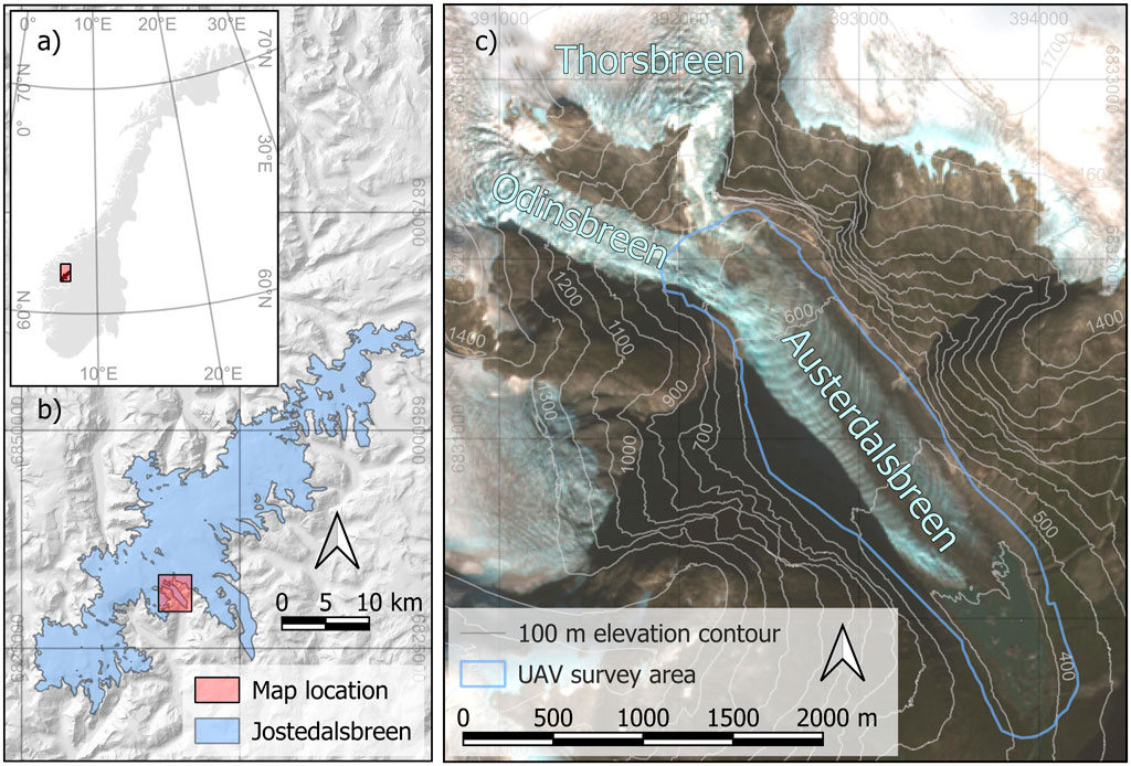
Figure 1. (a) Overview of the study area showing the location of the Jostedalsbreen ice cap in Norway; (b) the location of Austerdalsbreen in relation to the ice cap; and (c) a detail of Austerdalsbreen on 19 September 2024, showing the boundary of the UAV survey area. Notice the transverse light and dark bands called ogives on the glacier tongue. Satellite image: ESA (2024). Elevation data: Kartverket (2021) Glacier outlines: RGI Consortium (2023).
Several studies exist that focus on the glacier’s prominent ogives (transverse annual light and dark bands on the glacier surface, formed below the icefalls) and series of proglacial moraine ridges, and glacier dynamics were considered as a main influencing factor for explaining their formation and variability (King and Lewis, 1961; Eyles and Rogerson, 1978; Waddington, 1981). The surface of Austerdalsbreen is also characterized by a distinct ablation-dominated medial moraine, which separates the ice flow from the two icefalls. However, until now, no remote sensing-based approach to map glacier velocity with high-resolution data exists. Field observations show that the glacier is also characterized by a strong spatial variability in glacier velocity, from 5 m/yr at the ice margins to more than 100 m/yr near the icefalls, a distinctive feature already mentioned in the King and Lewis (1961). These spatio-temporal variations in glacier velocity, together with rapid surface changes, make Austerdalsbreen an ideal test site to study different velocity mapping techniques in challenging conditions.
2.2 Datasets and preprocessing
To test various glacier velocity algorithms, optical high-resolution UAV data is the main data source of this study. Furthermore, the integration of two additional optical remote sensing sensors intends to provide a feasible comparison to other datasets. We selected Sentinel-2 imagery as a medium resolution source to include one of the most used optical remote sensing sensors for glacier velocity mapping (Altena et al., 2019; Bhambri et al., 2020; Pronk et al., 2021; Zhou et al., 2021; Millan et al., 2022; Mouginot et al., 2023). To also provide an example of a high-resolution, spaceborne sensor, we also incorporated PlanetScope data into our analysis, which has been frequently used to calculate glacier velocity in existing research (Dell et al., 2019; Bhushan et al., 2020; Liu et al., 2020; Liu et al., 2024; Aati et al., 2022a; He et al., 2023).
2.2.1 UAV data - mapping and preprocessing
We performed one UAV flight on 13 September 2023 (1043 images), which is approximately at the end of the hydrological year that is also used for evaluating the mass balance of glaciers (Seibert et al., 2021) and one flight on 03 July 2024 (862 images), as prolonged snow cover makes earlier observations not feasible. However, the resulting time period from fall to early summer is an ideal benchmark for testing different sensors and algorithms, as it represents the winter period but also uses dates without snow cover, which may confound displacement calculations. Both datasets were acquired using a Wingtra Gen II fixed-wing UAV with a front and side overlap of 70% to ensure comprehensive coverage and high-quality photogrammetric reconstruction.
To accurately georeference the images, a Post-Processing Kinematics (PPK) workflow was applied, utilizing the Tunsbergsdalen base station, maintained by the Norwegian Mapping Authorities (Kartverket). This workflow resulted in geolocation residuals of 0.06 m in the X and Y directions and 0.11 m in the Z dimension for the 2023 acquisition, and 0.04 and 0.10 m for the 2024 acquisition.
The acquired images were processed photogrammetrically in Agisoft Metashape Professional following a standard workflow, beginning with image alignment and subsequent steps for 3D reconstruction.
The resulting orthophotos with a ground sampling distance of 0.03–0.04 m were then coregistered using an affine transformation with 14 manually mapped matching points, placed on solid surfaces along the glacier and lake boundary, leading to a registration error of 0.09 m. Finally, we resampled the images to 0.10 m, 0.15 m and 0.60 m for the analysis. This was performed to test different resolutions and to reduce processing times.
2.2.2 PlanetScope
The newest generation of the PlanetScope dove constellation is the PSB. SD instrument, which provides eight spectral bands (coastal blue, blue, green I, green, red, yellow, red edge and near-infrared (NIR)), a product resolution of 3 m, resampled from original 3–4 m depending on flight height, and near daily temporal resolution since 2021 (Planet Labs PBC, 2023). To reach the best possible match to the UAV campaign, we downloaded PlanetScope PSB. SD SuperDove ortho scene surface reflectance products (Planet Labs PBC, 2024) for 13 September 2023, and 20 July 2024. This is the closest possible match (within 17 days of the UAV acquisition) due to cloud coverage. Final products showed good coregistration, so no further geometrical corrections were applied.
2.2.3 Sentinel-2
Sentinel-2 provides 10 m spatial resolution with the blue, green, red and NIR bands and a revisit period of approximately 5 days. We used Level-1C data (ESA, 2024) to avoid potential artefacts from atmospheric corrections. The acquisition dates of the utilized scenes were 31 August 2023, and 24 June 2024. Respective dates represent the closest match to UAV acquisitions (within 13 and 9 days of the UAV images) without cloud cover or noise from haze. Visual inspection showed good geometrical coregistration and no further geometrical processing was performed. For some algorithms, respective data was resampled to 5 m to allow more flexibility with the step size.
2.3 Glacier surface velocity algorithms
The main target parameter of this study is horizontal (2D) displacement instead of 3D displacement, as the latter is also dependent on the quality of the associated digital elevation model, which complicates the assessment and is not available for the dates of the spaceborne data. We aimed at selecting algorithms that cover different methods, i.e., intensity tracking based on cross-correlation and feature tracking approaches, and that are applicable without the need of additional filtering, as this also introduces different tradeoffs and variations based on glacier shape and surface conditions (e.g., snow cover, shadows) during image acquisition (Paul et al., 2017). However, different algorithms lead to different output products, i.e., either raster datasets or displacement vectors. The latter have to be interpolated to provide a feasible comparison in the raster domain. In such situations, we used inverse distance weighted (IDW) for interpolation as this method is frequently used to interpolate glacier velocities from point data (Waechter et al., 2015) and shows good results and higher performance compared to other techniques (Gong et al., 2014; Hodam et al., 2017). The corresponding IDW-radius was set to half the maximum distance of resulting displacement vectors on the glacier surface to minimize holes in the interpolated surface. However, it is important to consider that the performance of interpolation techniques can be highly variable (Strößenreuther et al., 2020). To provide a comparison of all datasets in the vector domain, we calculated 100 m × 100 m median vectors from the resulting products.
2.3.1 Intensity tracking using geoCosiCorr3D
Intensity tracking methods compare small sections of images, called windows or chips, and correlate them to derive offsets that represent glacier velocities. We selected Geospatial CosiCorr3D (Aati et al., 2022b; Aati, 2024) because it is a newer improvement of the frequently used and cited COSI-Corr algorithm (Leprince et al., 2007; Heid and Kääb, 2012; Jawak et al., 2018). With this approach, horizontal 2D displacements are derived using a multi-scale moving window, whereby the first window maximizes the correlation between base and target image and a smaller window is used to compute a finer offset value. This correlation can be computed in both the spatial and the frequency domain, although the latter is recommended (Aati et al., 2022b). Several parameters need to be defined, such as the initial and final window sizes, number of iterations, and sampling distance. Sampling distance (step size) has to be larger than one pixel for this algorithm. To achieve a resolution higher than 20 m with the Sentinel-2 dataset, the mentioned resampling step to 5 m was performed. This approach usually uses a single band for each image. Therefore, we computed principal components with all our datasets, using all bands from PlanetScope and the 10 m bands from Sentinel-2, which is recommended to enhance topographic features and reduce noise in ice velocity research (Bindschadler and Scambos, 1991; Fahnestock et al., 2016). We used the first principal component to calculate the displacement with geoCosiCorr3D.
For other parameters, we used the initial settings according to the relevant literature (Aati et al., 2022a; Aati et al., 2022b) such as a window size larger than the expected displacement (Dematteis et al., 2022). However, when no correlation, intense noise, or unrealistic results appeared, we gradually adapted the window size or used the spatial instead of the frequency domain. With these variations, we also intended to reduce the effects of different tradeoffs due to different window sizes (Paul et al., 2017). The final products of the algorithm were raster-based u and v components, which were converted to total horizontal displacement.
2.3.2 Feature tracking using ORB
Feature tracking algorithms identify certain distinctive features in the primary images based on different techniques that are independent of orientation or scale, store the identified features as keypoints, and try to identify these distinctive points by comparing them to keypoints of secondary images (Gabarró et al., 2023). We selected an ORB-based feature tracking method implemented in the python package SeaIceDrift (Muckenhuber et al., 2016; Korosov and Rampal, 2017; NERSC, 2018), as this package shows high accuracy and speed in cryospheric research, and ORB shows better performance compared to other traditional feature tracking methods such as SIFT or SURF (Rublee et al., 2011; Muckenhuber et al., 2016; Li et al., 2022). The approach is based on the FAST (Features from Accelerated Segment Test) keypoint detector that analyses the images on several scales and levels, while ORB adds a direction using intensity-weighted centroids, selects the best keypoints to subsequently match the features using a brute force matcher and the Hamming distance, and applies a ratio-test before accepting the best match (Muckenhuber et al., 2016). Finally, we calculated displacement vectors from the resulting coordinates of the matches. We did not apply the pattern matching option of the mentioned package, which is based on the cross-correlation technique (Korosov and Rampal, 2017), to avoid methodological overlaps with the intensity tracking approach of the previous chapter. However, selective test results of the pattern matching technique did not show any improvements of the results obtained by standalone feature tracking applied in the presented study.
Numerous parameters, such as the number of target features, the ratio threshold, pyramid levels, maximum expected displacement, or patch size, can be selected in the module. In this study, all recommended settings according to Muckenhuber et al. (2016) were used for the initial run, apart from the expected displacement, which was set to the maximum observed value found in the literature (King and Lewis, 1961). In case of a low number of computed displacement vectors, we fine-tuned other parameters, e.g., by increasing the number of target features, ratio thresholds or pyramid levels to achieve a maximum number of reasonable displacement vectors and ideal spatial distribution.
For deriving final displacement vectors, we used the coordinates of the resulting matches to calculate the u component, the v component and the total displacement with subsequent interpolation.
2.3.3 Deep learning-based feature tracking
Deep learning-based image matching and feature tracking show increased performance in recent literature (Wang et al., 2022; Petrakis and Partsinevelos, 2023; Hendrickx et al., 2024). New deep learning techniques are considered particularly useful for challenging regions, such as mountain areas with steep topography, or given difficult conditions where traditional feature tracking methods may fail, such as situations with strong appearance changes and high rotational deformations (Yuan et al., 2022; Maiwald et al., 2023; Ioli et al., 2024).
In this study, we used the feature matching algorithms SuperPoint, SuperGlue and LightGlue (DeTone et al., 2018; Sarlin et al., 2020; Lindenberger et al., 2023), as implemented in the python package ICEpy4D (Ioli et al., 2023a), as the respective matching algorithms were already successfully used in glacier or permafrost environments (Ioli et al., 2023b; 2024; Hendrickx et al., 2024), although not for deriving glacier surface velocities from orthoimages but for 3D terrain reconstruction.
The approach uses single or three band images in byte format, and looks for corresponding points, which are detected by SuperPoint, and matches these points with the SuperGlue or LightGlue matcher (Ioli et al., 2023a; Lindenberger et al., 2023). SuperPoint is a Convolutional Neural Network (CNN) that uses a self-supervised training approach to extract relevant distinctive points in the images and a corresponding 256 unit descriptor, showing increased performance when compared to LIFT, SIFT and ORB (DeTone et al., 2018). SuperGlue then matches the keypoints using two components, an attentional graph neural network that uses initial features communicating with each other using self- and cross-attention layers for more robust representations of the descriptors, and an optimal matching layer that creates a score matrix to find the best partial assignment of the keypoints by utilizing the Sinkhorn algorithm (Sarlin et al., 2020). Thereby, the algorithm considers both images at the same time for outlier minimization and sparse point matching (Lindenberger et al., 2023). ICEpy4D uses pre-trained models with either indoor or outdoor-based sets of weights (Ioli et al., 2024). We selected the outdoor-based model, which is trained on the MegaDepth dataset (Li and Snavely, 2018) following (Ioli et al., 2024). In the case of a low number of matches, also the indoor model was tested, but this setting did not lead to improved results. The other utilized matcher, LightGlue, is an enhancement of SuperGlue that aims to make the feature tracking algorithm more accurate and efficient by preselecting points that are easier to match, and by discarding points that are considered not matchable by the algorithm (Lindenberger et al., 2023).
In addition to the selection of the indoor or outdoor pre-trained models, several options are available for fine tuning the feature matching approach, such as the SuperPoint keypoint detector threshold, the limit for the detected keypoints and tiled or untiled processing options. We used a tiled processing approach and a detector threshold of 0.0001 following recommendations in the package documentation (Ioli et al., 2023a), but we increased the limit for detected keypoints to 20,000.
For deriving final displacement vectors, we used the coordinates of the resulting matches to calculate the u component, the v component and the total displacement of the point-based displacements with subsequent interpolation.
2.4 Validation and performance measures
Different validation options for evaluating glacier velocities exist (Karimi et al., 2021; Mouginot et al., 2023; Liu et al., 2024) and several best practice approaches are discussed in Paul et al. (2017). Simple methods include visual inspections of the flow field and comparisons to the glacier outlines or inspections of stable ground areas. However, providing error measures based on ground-truth points from field surveys or higher resolution images are considered as the highest-level error assessment approaches (Paul et al., 2017). In this study, the applied approach followed these recommendations and included a combination of validation metrics.
Quantitative error measures are used as the most important indicators of algorithm performance following Paul et al. (2017). Therefore, the high-resolution UAV data (pixel size 3–4 cm) served as the basis for mapping displacement vectors across the glacier surface using distinctive features, a technique also used in previous research (Kraaijenbrink et al., 2016). Mapping was performed in a way where the search started at the confluence of the icefalls Thorsbreen and Odinsbreen towards the glacier terminus. After a distinctive feature was identified in both images and mapped in one glacier location in both images, the search continued about 100 m in the ice flow direction. The random and irregular nature of distinctive features together with the large surface change of the glacier led to several limitations, as it prevented a regular pattern of the resulting validation vectors and increased the originally intended mapping distance and density. In total, 43 validation vectors were mapped for most of the length of the glacier tongue covering different areas of the glacier surface. Although more vectors could theoretically be mapped in certain areas of the glacier, we avoided this practice and tried to maintain a balanced evaluation mapping along the whole length of the glacier, given the aforementioned limitations, to not bias the assessment towards areas where distinctive features were easier to map, as these areas most likely represented regions with lower surface changes and velocities.
The location of the mapped points was finally used to extract glacier velocities from the different algorithms. Due to the varying image capture dates, all displacements were converted to glacier velocity in m/yr for the final evaluation. Some velocity algorithms may lead to NA (no value is available) values on the glacier surface due to decorrelation of the image pairs. If ground-truth points were located in NA-areas, they were converted to zero before the evaluation to consider the same number of evaluation points for all algorithms. We calculated several performance measures frequently used in existing research to assess different algorithms and compare the results. The calculated measures were the root mean squared error (RMSE), the mean absolute error (MAE), and the bias. Additionally, we calculated respective relative values as a percentage of the mean measured glacier velocity. All performance measures were calculated according to formulas provided in Zandler et al. (2019).
In addition, visual inspection was used as a qualitative measure of algorithm performance as recommended in literature (Paul et al., 2017). We created maps of velocities, superimposed by calculated 100 m × 100 m median displacement vectors compared to the measured displacement vectors. Visual inspection of the algorithm results is important to quickly assess its capability to derive displacement patterns across the glacier or if it just generates random noise.
3 Results
The different sensors and algorithms, paired with the large number of modifiable settings (window and step size, keypoints, pyramid levels, detector thresholds) lead to a very large number of performance measures. Therefore, we only selected the best performing combinations for presentation in this section for a feasible comparison and we provide performance measures of other methods as a table in the Supplementary Material. An overview of algorithms, sensors, and main settings is summarized in Table 1 of chapter 3.5.

Table 1. Performance measures of different glacier velocity algorithms and sensors.R2.
3.1 UAV imagery comparison
Orthoimages of the flight campaign show a recession of the glacier tongue, an increase in debris cover, and substantial changes in the northwestern part of the glacier below the confluence of Thorsbreen and Odinsbreen (Figure 2). Mapped displacement vectors show glacier velocities between 5.3 m/yr and 105.6 m/yr (which translates to a displacement from 4.2 m to 85.0 m between the UAV survey periods) with an average value of 38.6 m/yr and a median value of 26.4 m/yr. Strong increases in surface velocity were visible towards Odinsbreen and Thorsbreen. Displacement vectors were mostly mapped along the medial moraine.
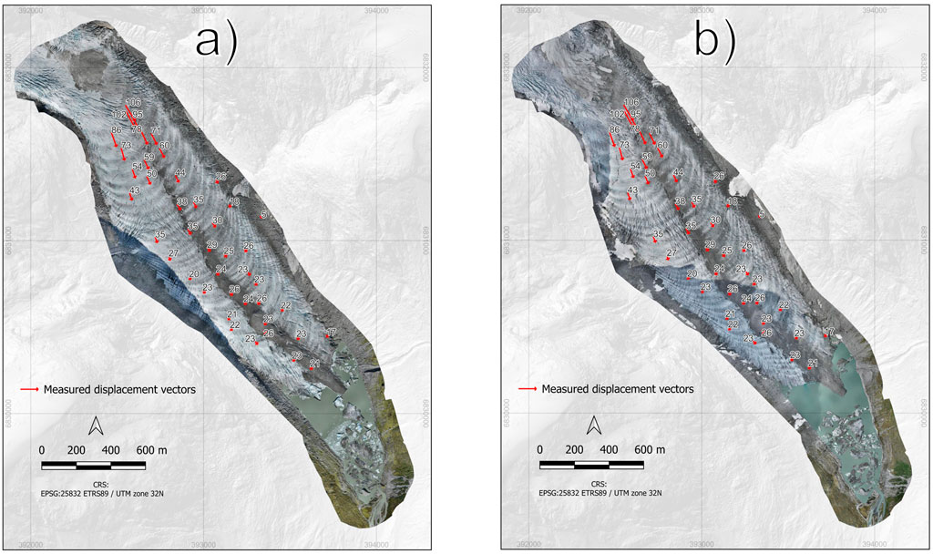
Figure 2. Orthoimages of Austerdalsbreen resulting from the survey flight on (a) 13 September 2023 and (b) 3 July 2024. Ground truth displacement vectors are shown on both images. The background hillshade is based on a DEM from 2020 (Kartverket, 2021).
3.2 GeoCosiCorr3D
With Sentinel-2, the intensity tracking method geoCosiCorr3D, with a window size of 32 × 32 pixels, a minimum step size of 10 m and based on the frequency domain, resulted in glacier velocity values throughout most of the glacier area (Figure 3). The algorithm produced low surface velocities near the glacier terminus with around 10 m/yr and higher values around 60 m/yr upglacier below the icefalls. Displacement direction was reasonably captured by the algorithm across most parts of the glacier. The glacier area below the icefalls was characterized by strong patchiness of the results with surface velocities alternating between 10 m/yr and more than 100 m/yr with several decorrelated areas without computed surface velocities. The same was true for larger stretches around the glacier periphery. Stable bedrock areas showed relatively high computed surface displacement values in some parts.
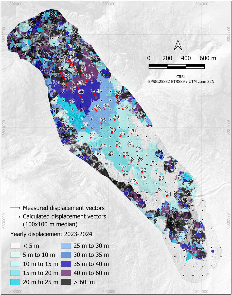
Figure 3. Displacement values based on Sentinel-2 imagery and the intensity tracking method geoCosiCorr3D compared to measured displacement vectors. Background hillshade shows UAV data 2023 on the glacier tongue and elevation in 2020 outside of the UAV survey area (Kartverket, 2021).
With PlanetScope data, geoCosiCorr3D led to the best results using a window size with a side length of 64 pixels and a minimum step size of 6 m. The algorithm resulted in glacier velocities across most parts of the glacier and a relatively smooth transition from lower velocities at the glacier terminus towards higher surface velocities below the icefalls (Figure 4). Directional vectors derived from the algorithm showed large agreement with mapped vectors. In the area closer to the icefalls, the results showed a noisy pattern and no clearly oriented vectors. Rocky areas next to the glacier partly resulted in no or almost no surface movement in some areas, but also several areas with computed movement and noise in the marginal parts of the glacier tongue.
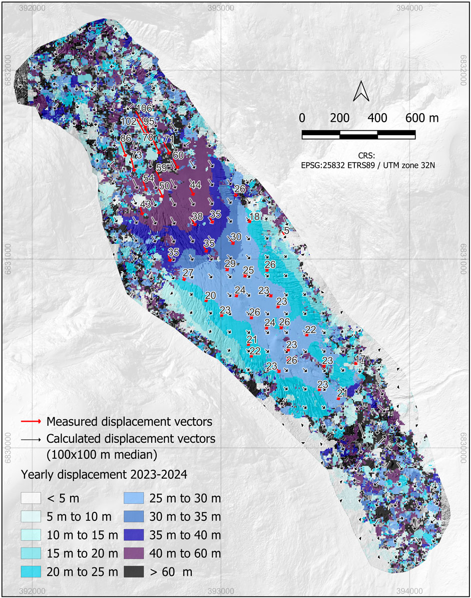
Figure 4. Displacement values based on PlanetScope imagery and the intensity tracking method geoCosiCorr3D compared to measured displacement vectors. Background hillshade shows UAV data 2023 on the glacier tongue and elevation in 2020 outside of the UAV survey area (Kartverket, 2021).
GeoCosiCorr3D applied to UAV data led to noisy results for large parts of the glacier surface with several window sizes (128 × 128 px, 256 × 256 px, 512 × 512 px) and resolutions (0.15 m and 0.60 m) using the frequency approach of geoCosiCorr3D. The “spatial” approach showed better and more stable results and best performance was achieved with the 0.6 m resolution, a window size of 64 pixels side length, and a maximum search range of 150 m (Figure 5). Visually, the results showed a smooth transition from the glacier terminus to the area with surface velocities of around 100 m/yr. Near the icefalls, the resulting displacement vectors were relatively chaotic while they showed mostly good agreement in other areas with exception of the medial moraine. The medial moraine also resulted in higher surface velocities than measured vectors. Stable areas were correctly mapped at the southeastern lake shore, but overestimated surface velocities occurred in other regions.
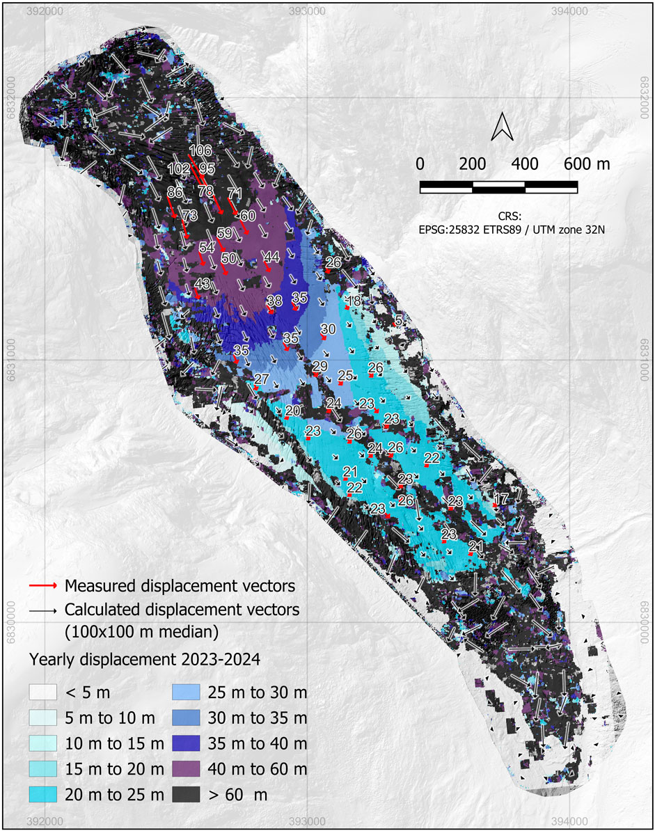
Figure 5. Displacement values based on UAV imagery and the intensity tracking method geoCosiCorr3D compared to measured displacement vectors. Background hillshade shows UAV data 2023 on the glacier tongue and elevation in 2020 outside of the UAV survey area (Kartverket, 2021).
3.3 ORB-based feature tracking (SeaIceDrift)
Feature tracking approaches with ORB did produce almost no displacement vectors with Sentinel-2 image pairs and were not further evaluated. Therefore, the feature tracking method was not applicable for this dataset and resolution. Similarly, ORB-based feature tracking did result in a very low number of displacement vectors with PlanetScope imagery, whereby some showed visual agreement to the mapped vectors, but most vectors showed no clear patterns and large deviations to the mapping results and glacier outline. Therefore, the results from ORB were not further analyzed and not feasible in combination with PlanetScope data.
Feature tracking based on ORB using UAV data did not result in sufficient displacement vectors with most settings. The best results were achieved with a resolution of 0.15 m, a ratio threshold of 0.9, and 250.000 target features (Figure 6). Thereby, many areas were not covered by displacement vectors. The remaining areas showed a transition from surface velocities of 20 m/yr at the terminus to maximum values of about 70 m/yr below the icefalls, while the produced displacement vectors showed similar direction compared to mapped displacements.
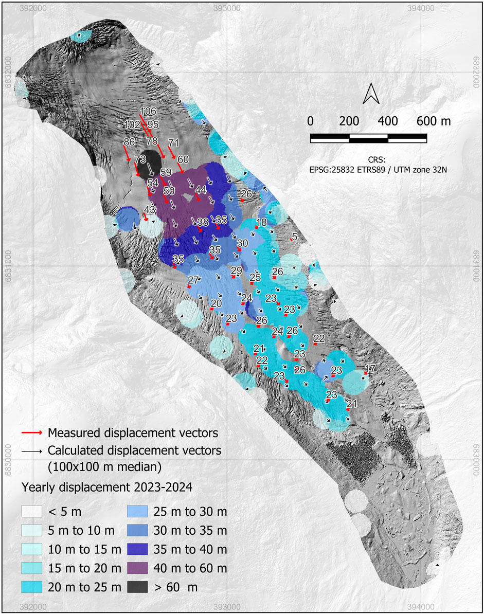
Figure 6. Displacement values based on UAV imagery and the feature tracking method ORB as implemented in SeaIceDrift compared to measured displacement vectors. Background hillshade shows UAV data 2023 on the glacier tongue and elevation in 2020 outside of the UAV survey area (Kartverket, 2021).
3.4 Deep learning-based feature tracking (ICEpy4D)
Sentinel-2 data did not result in a meaningful number of displacement vectors with deep learning techniques as implemented in ICEpy4D, rendering both tested feature tracking approaches not feasible with medium resolution optical data. The approach based on ICEpy4D, combining the SuperGlue and LightGlue matchers, computed glacier velocities in most areas with PlanetScope data, but also showed some irregular features and patchiness with strong velocity variations in some parts of the glacier (Figure 7).
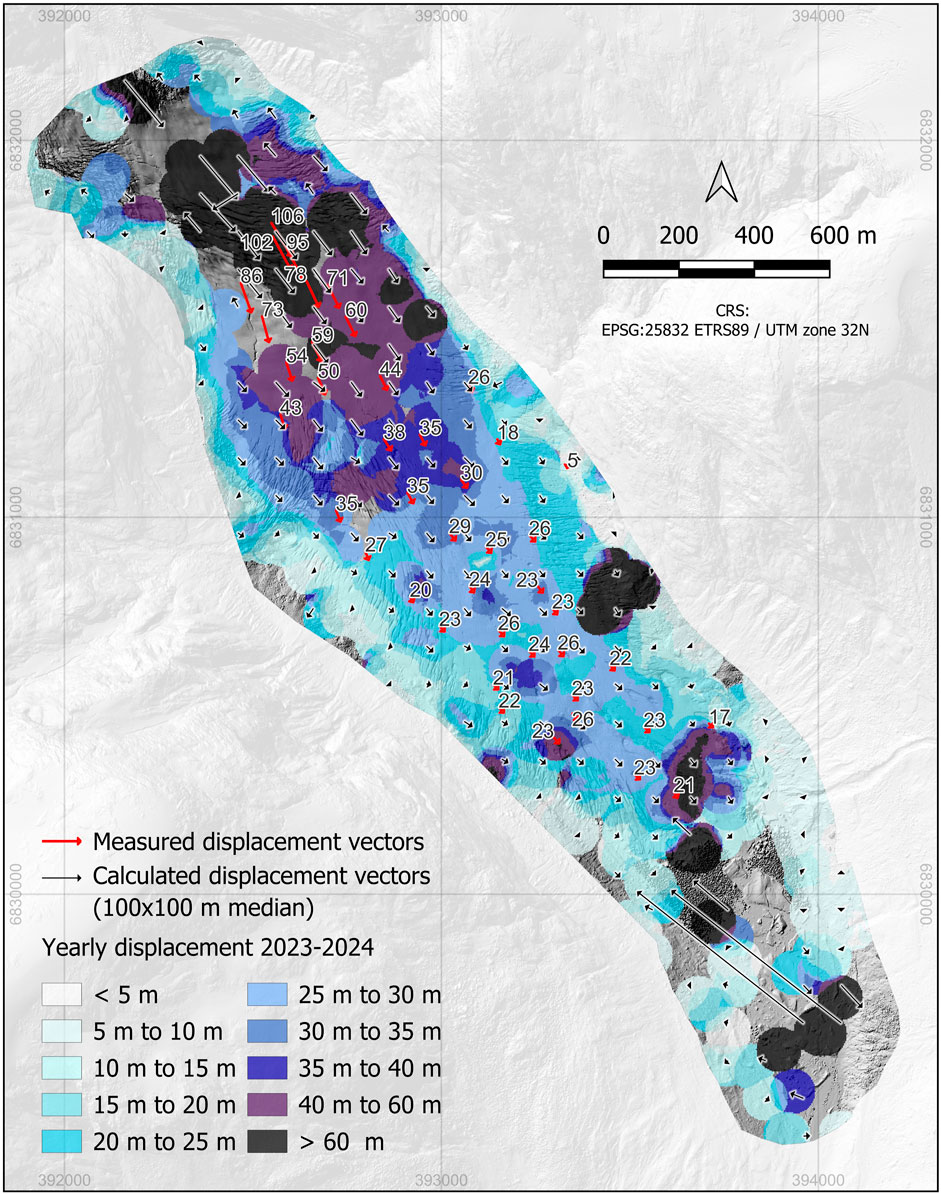
Figure 7. Displacement values based on PlanetScope imagery and the deep learning-based feature tracking method from ICEpy4D compared to measured displacement vectors. Background hillshade shows UAV data 2023 on the glacier tongue and elevation in 2020 outside of the UAV survey area (Kartverket, 2021).
Visual comparison of calculated directions to mapped directions showed a relatively good agreement until manually mapped surface speed of about 70 m/yr, but low agreement below the icefalls where higher speeds were mapped. Stable areas were often not correctly mapped and resulted in low surface displacements in most parts.
With UAV data, the deep learning algorithm resulted in calculated surface velocities across most parts of the glacier surface except directly below the icefalls, and a smooth transition between the different velocity classes is evident (Figure 8).
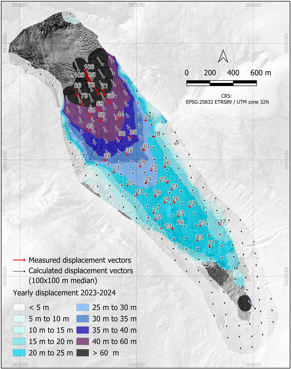
Figure 8. Displacement values based on UAV imagery and the deep learning-based feature tracking method from ICEpy4D compared to measured displacement vectors. Background hillshade shows UAV data 2023 on the glacier tongue and elevation in 2020 outside of the UAV survey area (Kartverket, 2021).
Best results were achieved with a combination of the SuperGlue and LightGlue matchers and both the 10 cm and 60 cm resolutions, whereby SuperGlue resulted in more matches on the glacier and LightGlue produced more displacement vectors in stable areas. Velocities around zero were calculated along the rocky stable areas around the glacier with some exceptions. The lake area at the glacier terminus showed an area of exceptionally high surface velocities. Almost all computed vectors matched mapped vectors in direction and length with the exception of water surfaces.
The qualitative comparison of all sensors showed a pattern with best results of the UAV data combined with deep learning-based feature tracking from ICEpy4D, followed by geoCosiCorr3D using PlanetScope and Sentinel-2, whereas geoCosiCorr3D with UAV imagery, the deep learning-based feature tracking method with PlanetScope data or the ORB feature tracking method as implemented in SeaIceDrift with UAV imagery resulted in many areas without appropriate detection of surface velocities (Figure 9).
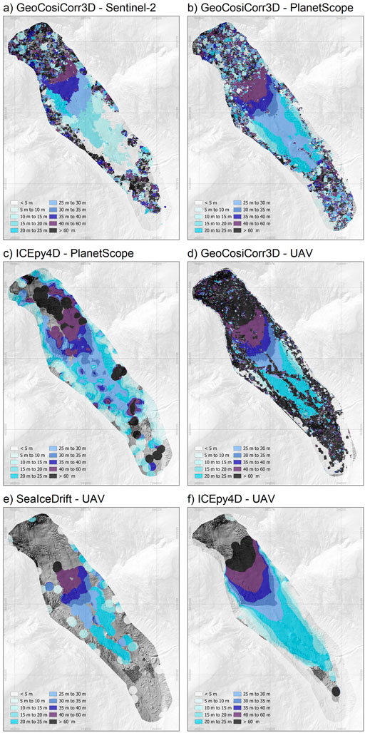
Figure 9. Visual comparison of resulting velocities of the different platforms and algorithms with (a) geoCosiCorr3D using Sentinel-2; (b) geoCosiCorr3D using PlanetScope; (c) ICEpy4D using PlanetScope; (d) geoCosiCorr3D using UAV data; (e) SeaIceDrift using UAV data; and (f) ICEpy4D using UAV data.
3.5 Performance measures of the algorithms and sensors
UAV data combined with deep learning-based feature tracking achieved the best results across all performance measures (Table 1). Sentinel-2 together with the intensity tracking method geoCosiCorr3D resulted in second highest R2 and second lowest RMSE, while PlanetScope with deep learning-based feature tracking or intensity tracking were second in respect to MAE and Bias. Lowest performances were achieved with UAV data using both intensity and ORB-based feature tracking methods, with relative RMSE errors of 94% to more than 100%.
Visual comparison of scatterplots supported numerical performance measures, with a constant negative Bias of the Sentinel-2 results, whereas the majority of data points were close to the 1:1 line with all other approaches with strong deviations particularly for intensity and ORB feature tracking methods with UAV data (Figure 10). GeoCosiCorr3D showed better matches at medium velocities with space-borne sensors, but higher errors at regions with lower or very high surface displacements.
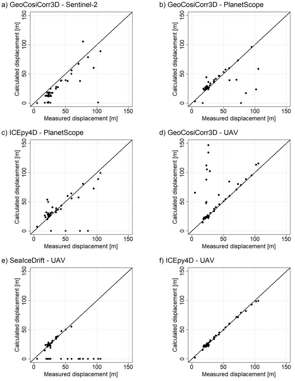
Figure 10. Scatterplots of measured compared to calculated displacement from the different platforms and algorithms with (a) geoCosiCorr3D using Sentinel-2; (b) geoCosiCorr3D using PlanetScope; (c) ICEpy4D using PlanetScope; (d) geoCosiCorr3D using UAV data; (e) SeaIceDrift using UAV data; and (f) ICEpy4D using UAV data.
The graphical comparison of differences between algorithm-based velocities and measured velocities also shows that outliers had a strong impact on error measures of several algorithms, particularly on GeoCosiCorr3D and ICEpy4D with PlanetScope, while the deep learning-based technique showed low differences to measured data and no outliers with UAV imagery (Figure 11). Sentinel-2 results showed a relatively low number of outliers and constant negative differences for most validation vectors. Methods using GeoCosiCorr3D and SeaIceDrift with UAV data generally showed higher error with particularly high errors of several outliers.
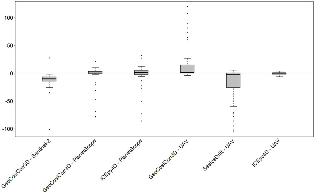
Figure 11. Boxplots of differences between yearly displacements as calculated with the applied algorithms versus measured yearly displacement values. Negative differences indicate lower algorithm velocities, while positive values indicate higher values of the calculated velocities.
4 Discussion
To our knowledge, this study is the first comparison of traditional tracking methods and innovative new deep learning feature tracking approaches for mapping glacier velocities from air- and spaceborne imagery. At the case study site of Austerdalsbreen, which is characterized by a highly dynamic ice surface for a land-based glacier, our results indicate that deep learning-based feature tracking outperforms traditional algorithms such as intensity tracking methods if applied to high-resolution UAV datasets. Quantitatively, the deep learning-based approach had sixteen times lower RMSE compared to the cross-correlation method. This result adds to the findings of existing research highlighting the potential of deep learning-based matching for surface dynamics of glaciers or permafrost environments (Hendrickx et al., 2024; Ioli et al., 2024).
4.1 Overall performance
With absolute error values of around 2 m/yr, the best results show considerable uncertainties and are higher compared to UAV-based results for very slow-moving glaciers (<10 m/yr) that resulted in errors around or below 1 m/yr (Cao et al., 2021; Karimi et al., 2021; Karimi, 2022). However, if relative errors are considered, the algorithm shows equally good performance with relative errors below 10% even under the challenging conditions of the local glacier dynamics, i.e., large velocity variations and considerable changes in surface features. Comparisons to evaluations in regions with moderate glacier velocities (<55 m), resulting in RMSE values of 1.7 m/yr to 1.9 m/yr (Van Tricht et al., 2021), also indicates the good performance of the presented method at higher surface velocities. Deep learning-based techniques were also applicable to PlanetScope data with coarser spatial resolution to some extent with a RMSE of 21 m/yr, a reasonable performance if compared to existing work using this sensor with cross-correlation methods (Liu et al., 2024). However, although these comparisons show the applicability of the deep learning-based feature tracking approach for UAV data, it must be stated that direct comparisons to other studies and evaluation approaches are challenging due to the different study settings.
Although the performance was lower than the deep learning-based UAV method, other algorithms achieved good results as well, but with different sensors. Intensity tracking, i. e., traditional cross correlation, showed MAE values around 14 m/yr with Sentinel-2, which is similar compared to existing medium resolution sensor studies, which reported errors of about 10 m/yr (Millan et al., 2022; Mouginot et al., 2023). However, RMSE values were higher in this study with 21 m/yr due to the impacts of validation points in glacier regions with high surface velocities. The comparison to research on faster glaciers (>70 m/yr) reporting RMSE values of >90 m/yr (Kelly et al., 2023), indicates superior performance of the presented study with medium resolution data. GeoCosiCorr3D also resulted in comparably good results with PlanetScope imagery, showing a RMSE of 22.5 m/yr, which is lower if compared to existing work on this sensor but also higher surface velocities (Liu et al., 2024).
4.2 Uncertainties and variability
Another notable result was that UAV derived datasets performed relatively poorly using existing, well-established methods, such as cross-correlation, in the presented setting. With intensity tracking methods, good results were achieved for bare ice areas with glacier velocities up to 60 m/yr. However, higher glacier velocities and areas with high debris cover, such as the medial moraine, led to decorrelation and no feasible velocity results, a result also reported by other UAV-based studies where decorrelation made intensity tracking impossible (Li et al., 2022). Changes in small features, such as rocks in the medial moraine, which are usually well visible in the high-resolution UAV data, but not in coarser resolution imagery, may therefore be a disadvantage for calculating surface displacement with such datasets. High displacements may also limit frequency-based intensity tracking approaches as reported by existing work (Dematteis et al., 2022). This is supported by the findings of the presented approach, where spatial and frequency-based methods showed similar results with space-borne sensors of lower resolution, but the spatial domain performed much better with UAV imagery. The relatively good performance of other sensors also showed that high-resolutions do not necessarily improve the performance, which is in line with the findings by Karimi (2022).
Deep learning-based feature tracking using UAV imagery led to the best performance at Austerdalsbreen, but was also connected to some variability of the results dependent on fine tuning of the algorithm. Combining the SuperGlue and LightGlue did not improve the quantitative performance measures, but resulted in more displacement vectors, particularly outside of the glacier area but also in high velocity regions. Therefore, some areas with high velocities, which result in a lower density of displacement vectors, are subject to considerable variability depending on the selected deep learning-based approach and respective settings. In the presented approach, LightGlue resulted in more matches in stable areas, as it preselects points, and discards points that are harder to match (Lindenberger et al., 2023). Therefore, the points that are harder to match are potentially found on areas with considerable surface changes, which were less prominent in the LightGlue approach compared to SuperGlue, while steady or more robust matches are more likely found on stable ground. In summary, the inhomogeneous density of matches resulting from the deep learning-based approach, as also visible in existing work (Ioli et al., 2023a; Ioli et al., 2024), is a clear disadvantage of the method compared to regular gridded approaches such as correlation-based intensity tracking. In this regard, the interpolation technique and associated parameters ads further variability and may introduce strange patterns, e.g., a bubbly appearance as visible on some feature tracking-based results, making the standardization and comparison of this approach difficult. Furthermore, higher resolutions may lead to a higher concentration of tie points in certain areas with good matches, whereas other areas with more challenging conditions may not be sufficiently covered, an issue that led to lower performance with higher resolved UAV imagery in this study.
The other tested feature tracking approach, ORB, did not produce a sufficient number of displacement vectors and was not successful in the presented study. Therefore, this method is not considered suitable for mapping glacier velocities in this setting. This result is unexpected, as this approach is frequently used for sea ice monitoring with medium resolution data (Hyun and Kim, 2018; Yang and Xie, 2024), and was also successfully used to match high-resolution images of rock glaciers (Marsy et al., 2020). Although results of the approach could be potentially improved using filtering of erroneous displacement vectors (Yang and Xie, 2024) or pairing it with correlation methods as implemented by the SeaIceDrift module (Muckenhuber et al., 2016), such an approach was not feasible in the presented approach given the low number of computed displacement vectors.
4.3 Algorithm comparison
Intensity tracking methods performed well in regions with small optical changes, which can be explained by the high correlation of regular tiles with a defined side length in such areas due to low changes in their grey value distributions (Leprince et al., 2007). Surface changes, rotations and changes in surface debris between acquisitions substantially change the overall distribution of grey values leading to the decorrelation of the whole tile, even if small sections within the tile may still be similar (Dematteis et al., 2022). Therefore, this method was not successful in the upper part of the glacier. Similarly, feature tracking based on traditional methods, such as the presented ORB algorithm, requires regular grey value distributions around the keypoints and complex distortions, missing content and occlusion inhibit the performance of this approach (Ioli et al., 2024). This partly explains the low performance of the ORB based technique. In contrast, techniques that are directly trained on data with challenging geometries to identify and match keypoints and include self- and cross attention layers, as the presented deep learning-based method, are particularly successful in situations of varying radiometry, illumination, different viewing angles and rotational deformations (Maiwald et al., 2021; Ioli et al., 2024; Morelli et al., 2024). All these conditions are frequently found in high-resolution imagery of glaciers due to rotations of single rocks, structural ice changes, illumination effects on the ice due to varying irradiance on the highly reflective ice surface and changes in sediment content. Furthermore, an important advantage of this technique is that it is based on keypoints and not a fixed window size, which is particularly important in regions where substantial changes occur and just small features are retained.
4.4 Relevance for glacier research
Our results showed that established cross-correlation methods performed well where glacier surface velocities are moderate and with imagery from medium to high-resolution, spaceborne sensors. However, neither areas with high velocities nor areas with very slow surface displacement were adequately resolved by these approaches. In contrast, glacier surfaces characterized by very low and very high velocities were successfully mapped using deep learning-based feature tracking and UAV data, and this technique was the only method that resulted in reasonable surface displacement results with the UAV imagery across the whole glacier. Therefore, the presented deep learning approach may be particularly useful in situations of large variabilities in glacier velocities, for detecting inter-seasonal glacier dynamics, or if large surface changes are present due to rotational transformation or ablation, for example, (Kraaijenbrink et al., 2016; Ioli et al., 2024). Additionally, this deep learning workflow may also be crucial for glaciological applications where small-scale processes are investigated with recourse to surface velocities, such as for sudden and intense accelerations of ice margins related to the drainage of ice-contact lakes (Bhardwaj et al., 2016; Mallalieu et al., 2017), ice passage through icefalls, or ice flow near calving fronts.
5 Conclusion
Traditional intensity tracking methods applied to high-resolution UAV data, such as cross-correlation, are suitable methods where glacial surface displacements are regular and relatively low (Vivero and Lambiel, 2019; Puniach et al., 2021). However, resolving ice surface velocities in areas of rapid changes in glacier surface conditions and in areas with high spatial variability in velocities can benefit from improved methods such as deep learning-based feature tracking. In this study, intensity tracking methods applied to datasets obtained from spaceborne sensors achieved good results for most parts of the glacier tongue of Austerdalsbreen, but could not resolve glacier velocities in areas characterized by strong surface changes. The applicability of methods is therefore mainly dependent on the rate of optical surface change and resolution, and intensity tracking methods are more suitable in situations where high temporal resolutions are possible during the snow free period.
This research illustrates the general feasibility of deep learning-based feature tracking for deriving glacier velocities using high-resolution remote sensing data. Respective technique substantially increases information on glacier surface velocities using high-resolution imagery, as it is able to deliver reliable displacement data in situations where traditional methods may fail. Therefore, the presented new deep image-matching method to derive glacier velocities implies a new level of detail in understanding and interpreting glacier dynamics. Improvements of deep learning-based feature tracking approaches, e.g., with more homogenous point densities, may greatly improve UAV-based velocity derivations under challenging conditions in future research.
Data availability statement
The datasets presented in this study can be found in online repositories. The names of the repository/repositories and accession number(s) can be found below: https://doi.org/10.5281/zenodo.14961373.
Author contributions
HZ: Conceptualization, Data curation, Formal Analysis, Investigation, Methodology, Resources, Software, Validation, Visualization, Writing – original draft, Writing – review and editing. JA: Conceptualization, Funding acquisition, Writing – original draft, Writing – review and editing. BR: Data curation, Funding acquisition, Investigation, Project administration, Writing - original draft, Writing – review and editing. AM: Writing – original draft, Writing – review and editing. TS: Funding acquisition, Writing – original draft, Writing – review and editing. JC: Funding acquisition, Writing – original draft, Writing – review and editing. JY: Funding acquisition, Project administration, Supervision, Writing – original draft, Writing – review and editing.
Funding
The author(s) declare that financial support was received for the research and/or publication of this article. Data acquisition for this study was funded by the Norwegian Research Council for the project JOSTICE (project no. 302458). Open access publishing was funded by the University of Graz.
Acknowledgments
We greatly appreciate funding of the JOSTICE project by the Norwegian Research Council, which enabled field work to generate UAV imagery for this publication. Thanks also go to Planet Labs PBC for making PlanetScope data freely available for the research community with their education and research program. Thanks also go to ESA for making remote sensing data freely available. Sven Le Moine-Bauer is thanked for participating in fieldwork in June 2024. The authors acknowledge the financial support by the University of Graz. Finally, we thank two reviewers for their efforts in improving our manuscript.
Conflict of interest
The authors declare that the research was conducted in the absence of any commercial or financial relationships that could be construed as a potential conflict of interest.
Generative AI statement
The author(s) declare that no Generative AI was used in the creation of this manuscript.
Publisher’s note
All claims expressed in this article are solely those of the authors and do not necessarily represent those of their affiliated organizations, or those of the publisher, the editors and the reviewers. Any product that may be evaluated in this article, or claim that may be made by its manufacturer, is not guaranteed or endorsed by the publisher.
Supplementary material
The Supplementary Material for this article can be found online at: https://www.frontiersin.org/articles/10.3389/frsen.2025.1586933/full#supplementary-material
References
Aati, S. (2024). Geospatial-COSICorr3D GitHub page. Available online at: https://github.com/SaifAati/Geospatial-COSICorr3D (Accessed January 16, 2025).
Aati, S., Avouac, J.-P., Rupnik, E., and Deseilligny, M.-P. (2022a). Potential and limitation of PlanetScope images for 2-D and 3-D earth surface monitoring with example of applications to glaciers and earthquakes. IEEE Trans. Geoscience Remote Sens. 60, 1–19. doi:10.1109/TGRS.2022.3215821
Aati, S., Milliner, C., and Avouac, J.-P. (2022b). A new approach for 2-D and 3-D precise measurements of ground deformation from optimized registration and correlation of optical images and ICA-based filtering of image geometry artifacts. Remote Sens. Environ. 277, 113038. doi:10.1016/j.rse.2022.113038
Altena, B., Haga, O. N., Nuth, C., and Kääb, A. (2019). Monitoring sub-weekly evolution of surface velocity and elevation for a high-latitude surging glacier using Sentinel-2. Int. Archives Photogrammetry, Remote Sens. Spatial Inf. Sci. XLII-2-W13, 1723–1727. doi:10.5194/isprs-archives-XLII-2-W13-1723-2019
Bhambri, R., Watson, C. S., Hewitt, K., Haritashya, U. K., Kargel, J. S., Pratap Shahi, A., et al. (2020). The hazardous 2017–2019 surge and river damming by Shispare Glacier, Karakoram. Sci. Rep. 10, 4685. doi:10.1038/s41598-020-61277-8
Bhardwaj, A., Sam, L., Akanksha, , Martín-Torres, F. J., and Kumar, R. (2016). UAVs as remote sensing platform in glaciology: present applications and future prospects. Remote Sens. Environ. 175, 196–204. doi:10.1016/j.rse.2015.12.029
Bhushan, S., Shean, D., Alexandrov, O., and Henderson, S. (2020). Automated tools to derive short-term glacier velocity from high-resolution commercial satellite imagery. Advance. Thousand Oaks, California, USA: Sage doi:10.1002/essoar.10502169.1
Bindschadler, R. A., and Scambos, T. A. (1991). Satellite-image-derived velocity field of an antarctic ice stream. Science 252, 242–246. doi:10.1126/science.252.5003.242
Cao, B., Guan, W., Li, K., Pan, B., and Sun, X. (2021). High-resolution monitoring of glacier mass balance and dynamics with unmanned aerial vehicles on the ningchan No. 1 glacier in the qilian mountains, China. Remote Sens. 13, 2735. doi:10.3390/rs13142735
Carrivick, J. L., Andreassen, L. M., Nesje, A., and Yde, J. C. (2022). A reconstruction of Jostedalsbreen during the Little Ice Age and geometric changes to outlet glaciers since then. Quat. Sci. Rev. 284, 107501. doi:10.1016/j.quascirev.2022.107501
Dell, R., Carr, R., Phillips, E., and Russell, A. J. (2019). Response of glacier flow and structure to proglacial lake development and climate at Fjallsjökull, south-east Iceland. J. Glaciol. 65, 321–336. doi:10.1017/jog.2019.18
Dematteis, N., Giordan, D., Crippa, B., and Monserrat, O. (2022). Fast local adaptive multiscale image matching algorithm for remote sensing image correlation. Comput. and Geosciences 159, 104988. doi:10.1016/j.cageo.2021.104988
DeTone, D., Malisiewicz, T., and Rabinovich, A. (2018). “SuperPoint: self-supervised interest point detection and description,” in 2018 IEEE/CVF conference on computer vision and pattern recognition workshops (CVPRW), 337–33712. doi:10.1109/CVPRW.2018.00060
ESA (2024). Copernicus Sentinel-2 data (processed by ESA). Available online at: https://browser.dataspace.copernicus.eu (Accessed December 05, 2025).
Eyles, N., and Rogerson, R. J. (1978). A framework for the investigation of medial moraine formation: austerdalsbreen, Norway, and berendon glacier, British columbia, Canada. J. Glaciol. 20, 99–113. doi:10.3189/S0022143000021249
Fahnestock, M., Scambos, T., Moon, T., Gardner, A., Haran, T., and Klinger, M. (2016). Rapid large-area mapping of ice flow using Landsat 8. Remote Sens. Environ. 185, 84–94. doi:10.1016/j.rse.2015.11.023
Friedl, P., Seehaus, T., and Braun, M. (2021). Global time series and temporal mosaics of glacier surface velocities derived from Sentinel-1 data. Earth Syst. Sci. Data 13, 4653–4675. doi:10.5194/essd-13-4653-2021
Gabarró, C., Hughes, N., Wilkinson, J., Bertino, L., Bracher, A., Diehl, T., et al. (2023). Improving satellite-based monitoring of the polar regions: identification of research and capacity gaps. Front. Remote Sens. 4. doi:10.3389/frsen.2023.952091
Gillespie, M. K., Andreassen, L. M., Huss, M., de Villiers, S., Sjursen, K. H., Aasen, J., et al. (2024). Ice thickness and bed topography of Jostedalsbreen ice cap, Norway. Earth Syst. Sci. Data 16, 5799–5825. doi:10.5194/essd-16-5799-2024
Gong, G., Mattevada, S., and O’Bryant, S. E. (2014). Comparison of the accuracy of kriging and IDW interpolations in estimating groundwater arsenic concentrations in Texas. Environ. Res. 130, 59–69. doi:10.1016/j.envres.2013.12.005
He, Z., Yang, W., Wang, Y., Zhao, C., Ren, S., and Li, C. (2023). Dynamic changes of a thick debris-covered glacier in the southeastern Tibetan plateau. Remote Sens. 15, 357. doi:10.3390/rs15020357
Heid, T., and Kääb, A. (2012). Evaluation of existing image matching methods for deriving glacier surface displacements globally from optical satellite imagery. Remote Sens. Environ. 118, 339–355. doi:10.1016/j.rse.2011.11.024
Hendrickx, H., Blanch, X., Elias, M., Delaloye, R., and Eltner, A. (2024). AI-based tracking of fast-moving alpine landforms using high frequency monoscopic time-lapse imagery. EGUsphere, 1–20. doi:10.5194/egusphere-2024-2570
Hodam, S., Sarkar, S., Marak, A. G. R., Bandyopadhyay, A., and Bhadra, A. (2017). Spatial interpolation of reference evapotranspiration in India: comparison of IDW and kriging methods. J. Inst. Eng. India Ser. A 98, 511–524. doi:10.1007/s40030-017-0241-z
Hyun, C.-U., and Kim, H. (2018). Arctic Sea ice motion measurement using time-series high-resolution optical satellite images and feature tracking techniques. Korean J. Remote Sens. 34, 1215–1227. doi:10.7780/kjrs.2018.34.6.2.6
Immerzeel, W. W., Kraaijenbrink, P. D. A., Shea, J. M., Shrestha, A. B., Pellicciotti, F., Bierkens, M. F. P., et al. (2014). High-resolution monitoring of Himalayan glacier dynamics using unmanned aerial vehicles. Remote Sens. Environ. 150, 93–103. doi:10.1016/j.rse.2014.04.025
Ioli, F., Barbieri, F., Gaspari, F., Nex, F., and Pinto, L. (2023a). ICEpy4D: a Python toolkit for advanced multi-epoch glacier monitoring with deepl-learning photogrammetry. Int. Archives Photogrammetry, Remote Sens. Spatial Inf. Sci. XLVIII-1-W2-2023, 1037–1044. doi:10.5194/isprs-archives-XLVIII-1-W2-2023-1037-2023
Ioli, F., Bruno, E., Calzolari, D., Galbiati, M., Mannocchi, A., Manzoni, P., et al. (2023b). A replicable open-source multi camera system for low-cost 4D glacier monitoring. Int. Archives Photogrammetry, Remote Sens. Spatial Inf. Sci. XLVIII-M (1–2023), 137–144. doi:10.5194/isprs-archives-XLVIII-M-1-2023-137-2023
Ioli, F., Dematteis, N., Giordan, D., Nex, F., and Pinto, L. (2024). Deep learning low-cost photogrammetry for 4D short-term glacier dynamics monitoring. PFG 92, 657–678. doi:10.1007/s41064-023-00272-w
Jawak, S. D., Kumar, S., Luis, A. J., Bartanwala, M., Tummala, S., and Pandey, A. C. (2018). “Evaluation of geospatial tools for generating accurate glacier velocity maps from optical remote sensing data,” in The 2nd international electronic conference on remote sensing (MDPI), Basel, Switzerland: MDPI 341. doi:10.3390/ecrs-2-05154
Jouvet, G., Weidmann, Y., Kneib, M., Detert, M., Seguinot, J., Sakakibara, D., et al. (2018). Short-lived ice speed-up and plume water flow captured by a VTOL UAV give insights into subglacial hydrological system of Bowdoin Glacier. Remote Sens. Environ. 217, 389–399. doi:10.1016/j.rse.2018.08.027
Karimi, N. (2022). Alpine glacier surface velocity measurement from UAV imagery – examining the effect of image resolution on the accuracy of results. Geocarto Int. 37, 10990–11009. doi:10.1080/10106049.2022.2043454
Karimi, N., Sheshangosht, S., and Roozbahani, R. (2021). High-resolution monitoring of debris-covered glacier mass budget and flow velocity using repeated UAV photogrammetry in Iran. Geomorphology 389, 107855. doi:10.1016/j.geomorph.2021.107855
Kartverket (2021). Høyde DOM1: 1 m digital surface model 2020. Lasercanning. Available online at: https://hoydedata.no/LaserInnsyn2/.
Kelly, J. T., Hehlen, M., and McGee, S. (2023). Uncertainty of satellite-derived glacier flow velocities in a temperate alpine setting (juneau icefield, Alaska). Remote Sens. 15, 3828. doi:10.3390/rs15153828
King, C. A. M., and Lewis, W. V. (1961). A tentative theory of ogive formation. J. Glaciol. 3, 912–939. doi:10.3189/S0022143000027283
Korosov, A. A., and Rampal, P. (2017). A combination of feature tracking and pattern matching with optimal parametrization for sea ice drift retrieval from SAR data. Remote Sens. 9, 258. doi:10.3390/rs9030258
Kraaijenbrink, P., Meijer, S. W., Shea, J. M., Pellicciotti, F., Jong, S. M. D., and Immerzeel, W. W. (2016). Seasonal surface velocities of a Himalayan glacier derived by automated correlation of unmanned aerial vehicle imagery. Ann. Glaciol. 57, 103–113. doi:10.3189/2016AoG71A072
Leprince, S., Barbot, S., Ayoub, F., and Avouac, J.-P. (2007). Automatic and precise orthorectification, coregistration, and subpixel correlation of satellite images, application to ground deformation measurements. IEEE Trans. Geoscience Remote Sens. 45, 1529–1558. doi:10.1109/TGRS.2006.888937
Li, G., Chen, Z., Mao, Y., Yang, Z., Chen, X., and Cheng, X. (2024a). Different glacier surge patterns revealed by Sentinel-2 imagery derived quasi-monthly flow velocity at west Kunlun Shan, Karakoram, Hindu Kush and Pamir. Remote Sens. Environ. 311, 114298. doi:10.1016/j.rse.2024.114298
Li, L., Yang, Y., Wang, S., Wang, C., Wang, Q., Chen, Y., et al. (2024b). Yearly elevation change and surface velocity revealed from two UAV surveys at baishui river glacier No. 1, yulong snow mountain. Atmosphere 15, 231. doi:10.3390/atmos15020231
Li, M., Zhou, C., Chen, X., Liu, Y., Li, B., and Liu, T. (2022). Improvement of the feature tracking and patter matching algorithm for sea ice motion retrieval from SAR and optical imagery. Int. J. Appl. Earth Observation Geoinformation 112, 102908. doi:10.1016/j.jag.2022.102908
Li, Z., and Snavely, N. (2018). “MegaDepth: learning single-view depth prediction from internet photos,” in 2018 IEEE/CVF Conference on computer Vision and pattern recognition, (salt lake city, UT, USA: ieee), 2041–2050. doi:10.1109/CVPR.2018.00218
Lindenberger, P., Sarlin, P.-E., and Pollefeys, M. (2023). LightGlue: local feature matching at light speed. doi:10.48550/arXiv.2306.13643
Liu, J., Gendreau, M., Enderlin, E. M., and Aberle, R. (2024). Improved records of glacier flow instabilities using customized NASA autoRIFT (CautoRIFT) applied to PlanetScope imagery. Cryosphere 18, 3571–3590. doi:10.5194/tc-18-3571-2024
Liu, Q., Mayer, C., Wang, X., Nie, Y., Wu, K., Wei, J., et al. (2020). Interannual flow dynamics driven by frontal retreat of a lake-terminating glacier in the Chinese Central Himalaya. Earth Planet. Sci. Lett. 546, 116450. doi:10.1016/j.epsl.2020.116450
Maiwald, F., Feurer, D., and Eltner, A. (2023). Solving photogrammetric cold cases using AI-based image matching: new potential for monitoring the past with historical aerial images. ISPRS J. Photogrammetry Remote Sens. 206, 184–200. doi:10.1016/j.isprsjprs.2023.11.008
Maiwald, F., Lehmann, C., and Lazariv, T. (2021). Fully automated pose estimation of historical images in the context of 4D geographic information systems utilizing machine learning methods. ISPRS Int. J. Geo-Information 10, 748. doi:10.3390/ijgi10110748
Mallalieu, J., Carrivick, J. L., Quincey, D. J., Smith, M. W., and James, W. H. M. (2017). An integrated Structure-from-Motion and time-lapse technique for quantifying ice-margin dynamics. J. Glaciol. 63, 937–949. doi:10.1017/jog.2017.48
Marsy, G., Vernier, F., Bodin, X., Cusicanqui, D., Castaings, W., and Trouvé, E. (2020). Monitoring mountain cryosphere dynamics by time lapse stereo photogrammetry. ISPRS Ann. Photogramm. Remote Sens. Spat. Inf. Sci. V-2–2020 V-2-2020, 459–466. doi:10.5194/isprs-annals-V-2-2020-459-2020
Millan, R., Mouginot, J., Rabatel, A., and Morlighem, M. (2022). Ice velocity and thickness of the world’s glaciers. Nat. Geosci. 15, 124–129. doi:10.1038/s41561-021-00885-z
Mohanty, A., Srivastava, P. K., and Aggarwal, A. (2024). Review of glacier velocity and facies characterization techniques using multi-sensor approach. Environ. Dev. Sustain. doi:10.1007/s10668-024-04604-7
Morelli, L., Ioli, F., Maiwald, F., Mazzacca, G., Menna, F., and Remondino, F. (2024). Deep-image-matching: a toolbox for multiview image matching of complex scenarios. Int. Archives Photogrammetry, Remote Sens. Spatial Inf. Sci., 309–316. XLVIII-2-W4-2024. doi:10.5194/isprs-archives-XLVIII-2-W4-2024-309-2024
Mouginot, J., Rabatel, A., Ducasse, E., and Millan, R. (2023). Optimization of cross correlation algorithm for annual mapping of alpine glacier flow velocities; application to sentinel-2. IEEE Trans. Geoscience Remote Sens. 61, 1–12. doi:10.1109/TGRS.2022.3223259
Muckenhuber, S., Korosov, A. A., and Sandven, S. (2016). Open-source feature-tracking algorithm for sea ice drift retrieval from Sentinel-1 SAR imagery. Cryosphere 10, 913–925. doi:10.5194/tc-10-913-2016
Nanni, U., Scherler, D., Ayoub, F., Millan, R., Herman, F., and Avouac, J.-P. (2023). Climatic control on seasonal variations in mountain glacier surface velocity. Cryosphere 17, 1567–1583. doi:10.5194/tc-17-1567-2023
NERSC (2018). GitHub page for the package SeaIceDrift-0.7. Nansen environmental and remote sensing center (NERSC). Contributors Ant. Korosov, Timothy Williams Ashwin Nair. Available online at: https://github.com/nansencenter/sea_ice_drift (Accessed January 17, 2025).
Pang, L., Yao, J., Li, K., and Cao, X. (2025). SPECIAL: zero-shot hyperspectral image classification with CLIP. doi:10.48550/arXiv.2501.16222
Paul, F., Bolch, T., Briggs, K., Kääb, A., McMillan, M., McNabb, R., et al. (2017). Error sources and guidelines for quality assessment of glacier area, elevation change, and velocity products derived from satellite data in the Glaciers_cci project. Remote Sens. Environ. 203, 256–275. doi:10.1016/j.rse.2017.08.038
Petrakis, G., and Partsinevelos, P. (2023). Keypoint detection and description through deep learning in unstructured environments. Robotics 12, 137. doi:10.3390/robotics12050137
Planet Labs PBC (2023). Planet imagery product specifications. Available online at: https://assets.planet.com/docs/Planet_Combined_Imagery_Product_Specs_letter_screen.pdf.
Planet Labs PBC (2024). Planet application program interface: in space for life on earth. Available online at: https://api.planet.com.
Pronk, J. B., Bolch, T., King, O., Wouters, B., and Benn, D. I. (2021). Contrasting surface velocities between lake- and land-terminating glaciers in the Himalayan region. Cryosphere 15, 5577–5599. doi:10.5194/tc-15-5577-2021
Puniach, E., Gruszczyński, W., Ćwiąkała, P., and Matwij, W. (2021). Application of UAV-based orthomosaics for determination of horizontal displacement caused by underground mining. ISPRS J. Photogrammetry Remote Sens. 174, 282–303. doi:10.1016/j.isprsjprs.2021.02.006
Qiao, G., Yuan, X., Florinsky, I., Popov, S., He, Y., and Li, H. (2023). Topography reconstruction and evolution analysis of outlet glacier using data from unmanned aerial vehicles in Antarctica. Int. J. Appl. Earth Observation Geoinformation 117, 103186. doi:10.1016/j.jag.2023.103186
RGI Consortium (2023). Randolph Glacier inventory - a dataset of global Glacier Outlines (NSIDC-0770, Version 7). doi:10.5067/F6JMOVY5NAVZ
Rippin, D. M., Pomfret, A., and King, N. (2015). High resolution mapping of supra-glacial drainage pathways reveals link between micro-channel drainage density, surface roughness and surface reflectance. Earth Surf. Process. Landforms 40, 1279–1290. doi:10.1002/esp.3719
Robson, B. A., MacDonell, S., Ayala, Á., Bolch, T., Nielsen, P. R., and Vivero, S. (2022). Glacier and rock glacier changes since the 1950s in the La Laguna catchment, Chile. Cryosphere 16, 647–665. doi:10.5194/tc-16-647-2022
Rounce, D. R., Hock, R., Maussion, F., Hugonnet, R., Kochtitzky, W., Huss, M., et al. (2023). Global glacier change in the 21st century: every increase in temperature matters. Science 379, 78–83. doi:10.1126/science.abo1324
Rublee, E., Rabaud, V., Konolige, K., and Bradski, G. (2011). “ORB: an efficient alternative to SIFT or SURF,” in 2011 international conference on computer vision, 2564–2571. doi:10.1109/ICCV.2011.6126544
Sarlin, P.-E., DeTone, D., Malisiewicz, T., and Rabinovich, A. (2020). SuperGlue: learning feature matching with graph neural networks, 4937, 4946. doi:10.1109/cvpr42600.2020.00499
Scambos, T. A., Dutkiewicz, M. J., Wilson, J. C., and Bindschadler, R. A. (1992). Application of image cross-correlation to the measurement of glacier velocity using satellite image data. Remote Sens. Environ. 42, 177–186. doi:10.1016/0034-4257(92)90101-O
Seibert, J., Jenicek, M., Huss, M., Ewen, T., and Viviroli, D. (2021). “Chapter 4 - snow and ice in the hydrosphere,” in Snow and ice-related hazards, risks, and disasters. Editors W. Haeberli, and C. Whiteman Second Edition (Elsevier), 93–135. doi:10.1016/B978-0-12-817129-5.00010-X
Seier, G., Abermann, J., Andreassen, L. M., Carrivick, J. L., Kielland, P. H., Löffler, K., et al. (2024). Glacier thinning, recession and advance, and the associated evolution of a glacial lake between 1966 and 2021 at Austerdalsbreen, western Norway. Land Degrad. Dev. 35, 394–414. doi:10.1002/ldr.4923
Shen, H., Zhou, S., Fang, L., and Yang, J. (2022). Glacier motion monitoring using a novel deep matching network with SAR intensity images. Remote Sens. 14, 5128. doi:10.3390/rs14205128
Shukla, A., and Garg, P. K. (2019). Evolution of a debris-covered glacier in the western Himalaya during the last four decades (1971–2016): a multiparametric assessment using remote sensing and field observations. Geomorphology 341, 1–14. doi:10.1016/j.geomorph.2019.05.009
Sood, S., Thakur, P. K., Stein, A., Garg, V., and Dixit, A. (2022). Mapping Samudra Tapu glacier: a holistic approach utilizing radar and optical remote sensing data for glacier radar facies mapping and velocity estimation. Adv. Space Res. 70, 3975–3999. doi:10.1016/j.asr.2022.10.030
Strößenreuther, U., Horwath, M., and Schröder, L. (2020). How different analysis and interpolation methods affect the accuracy of ice surface elevation changes inferred from satellite altimetry. Math. Geosci. 52, 499–525. doi:10.1007/s11004-019-09851-3
Tang, D., Cao, X., Wu, X., Li, J., Yao, J., Bai, X., et al. (2025). AeroGen: enhancing remote sensing object detection with diffusion-driven data generation. doi:10.48550/arXiv.2411.15497
Van Tricht, L., Huybrechts, P., Van Breedam, J., Vanhulle, A., Van Oost, K., and Zekollari, H. (2021). Estimating surface mass balance patterns from unoccupied aerial vehicle measurements in the ablation area of the Morteratsch–Pers glacier complex (Switzerland). Cryosphere 15, 4445–4464. doi:10.5194/tc-15-4445-2021
Van Wyk De Vries, M., and Wickert, A. D. (2021). Glacier Image Velocimetry: an open-source toolbox for easy and rapid calculation of high-resolution glacier velocity fields. Cryosphere 15, 2115–2132. doi:10.5194/tc-15-2115-2021
Vivero, S., and Lambiel, C. (2019). Monitoring the crisis of a rock glacier with repeated UAV surveys. Geogr. Helv. 74, 59–69. doi:10.5194/gh-74-59-2019
Waddington, E. D. (1981). Accurate modelling of glacier flow. Vancouver, Canada: University of British Columbia. doi:10.14288/1.0052458
Waechter, A., Copland, L., and Herdes, E. (2015). Modern glacier velocities across the icefield ranges, st elias mountains, and variability at selected glaciers from 1959 to 2012. J. Glaciol. 61, 624–634. doi:10.3189/2015JoG14J147
Wang, L., Lan, C., Wu, B., Gao, T., Wei, Z., and Yao, F. (2022). A method for detecting feature-sparse regions and matching enhancement. Remote Sens. 14, 6214. doi:10.3390/rs14246214
Wang, P., Li, H., Li, Z., Liu, Y., Xu, C., Mu, J., et al. (2021). Seasonal surface change of urumqi glacier No. 1, eastern tien Shan, China, revealed by repeated high-resolution UAV photogrammetry. Remote Sens. 13, 3398. doi:10.3390/rs13173398
Yang, Y. L., and Xie, T. (2024). Sea ice drift vector extraction based on feature matching using CS-1 Images. J. Phys. Conf. Ser. 2718, 012012. doi:10.1088/1742-6596/2718/1/012012
Yuan, X., Yuan, X., Chen, J., and Wang, X. (2022). Large aerial image tie point matching in real and difficult survey areas via deep learning method. Remote Sens. 14, 3907. doi:10.3390/rs14163907
Zandler, H., Haag, I., and Samimi, C. (2019). Evaluation needs and temporal performance differences of gridded precipitation products in peripheral mountain regions. Sci. Rep. 9, 15118. doi:10.1038/s41598-019-51666-z
Zhou, W., Xu, M., and Han, H. (2024). Spatial distribution and variation in debris cover and flow velocities of glaciers during 1989–2022 in tomur peak region, tianshan mountains. Remote Sens. 16, 2587. doi:10.3390/rs16142587
Keywords: UAV, PlanetScope, Sentinel-2, cross-correlation, Superpoint, SuperGlue, LightGlue, displacement
Citation: Zandler H, Abermann J, Robson BA, Maschler A, Scheiber T, Carrivick JL and Yde JC (2025) Deep learning outperforms existing algorithms in glacier surface velocity estimation with high-resolution data – the example of Austerdalsbreen, Norway. Front. Remote Sens. 6:1586933. doi: 10.3389/frsen.2025.1586933
Received: 03 March 2025; Accepted: 14 May 2025;
Published: 26 May 2025.
Edited by:
Sher Muhammad, International Centre for Integrated Mountain Development, NepalReviewed by:
Jing Yao, Chinese Academy of Sciences (CAS), ChinaKonstantin Maslov, University of Twente, Netherlands
Copyright © 2025 Zandler, Abermann, Robson, Maschler, Scheiber, Carrivick and Yde. This is an open-access article distributed under the terms of the Creative Commons Attribution License (CC BY). The use, distribution or reproduction in other forums is permitted, provided the original author(s) and the copyright owner(s) are credited and that the original publication in this journal is cited, in accordance with accepted academic practice. No use, distribution or reproduction is permitted which does not comply with these terms.
*Correspondence: Harald Zandler, aGFyYWxkLnphbmRsZXJAdW5pLWdyYXouYXQ=