Bare surface soil moisture and surface roughness estimation using multi-band multi-polarization NISAR-like SAR data

The upcoming NISAR Earth-observation satellite will utilize dual frequencies simultaneously, providing synthetic aperture radar (SAR) remote sensing data in both the L-band and S-band. With its ability to operate single-polarization, dual-polarization, and quad-polarization modes, NISAR will offer significant capabilities for land surface observation applications, particularly for estimating surface soil moisture (SSM) and surface roughness (Hrms). This study aims to demonstrate NISAR’s future potential in SSM and Hrms estimation by evaluating the single (SP), double (DP) and quad (QP) polarization configurations. Noisy synthetic NISAR-like data was generated using the Dubois-B model for both S- and L-bands. The use of a priori information on the soil moisture was also examined for SSM and Hrms estimations. Various neural networks (NNs) were trained using the noisy synthetic dataset. Validation was performed on noisy synthetic data, as real NISAR data is not yet available. Out of the NISAR configurations tested, the QP configuration was shown to be the most performant, with RMSE on SSM estimation of 4.2 vol.%, for QP configuration compared to 5.1 and 8.2 vol.% for SP and DP configurations when not using a priori knowledge of soil moisture conditions. RMSE on Hrms was 0.3 cm for QP configuration, compared to 0.7 and 0.6 cm for SP and DP configurations. The QP was also shown to be more capable of mitigating the effect of the incidence angle on the estimation of SSM and Hrms compared to the two other configurations. Moreover, simultaneous use of S- and L-bands enhances SSM and Hrms estimation compared to using either of these frequency bands alone in single-, dual-, or quad-polarization configurations. Furthermore, using a priori knowledge of soil moisture conditions was successful in improving the estimation precision for SSM for all NISAR configurations. Notably, for QP configuration, RMSE on SSM estimation was 3.9 vol.% and 3.2 vol.% when a priori information on SSM was considered respectively in dry to slightly wet and very wet conditions. These findings demonstrate the high potential of the future NISAR sensor for estimating SSM and Hrms.

1 Introduction

Soil is the boundary layer between land and atmosphere, and represents the interface of interaction between the two (Camillo et al., 1983). Surface soil moisture (SSM) and soil roughness (represented by root mean square height, Hrms) are two soil parameters that are widely used in hydrology, agronomy and environment science (Engman, 1991; Jackson et al., 1996; Acutis and Donatelli, 2003; Vereecken et al., 2022). Traditionally, soil moisture is measured with ground measurement instruments, such as dielectric, capacitance, and neutron probes, with high accuracy; while surface roughness can be measured using profile meters, laser, and photogrammetry tools (Jester and Klik, 2005; Evett et al., 2008; Feidenhans’l et al., 2015). However, these traditional measurement tools have limitations as they can only measure the soil parameters at the point of measurement, potentially misrepresenting the wider area (spatial representation), and are time demanding and resource intensive, making operation challenging when used over larger areas.

In more recent works, radar remote sensing data have been used for estimating soil moisture and roughness through various approaches. There are currently numerous satellite missions used for soil parameter retrieval, some rely on passive radar technology (Kerr et al., 2016; Colliander et al., 2022), which generally have a low resolution, while others rely on active radar technology (Mirsoleimani et al., 2019; Gorrab et al., 2016; El Hajj et al., 2016; Ettalbi et al., 2023) and have higher resolution. Passive satellites, such as the Soil Moisture and Ocean Salinity (SMOS) mission, and the Soil Moisture Active Passive (SMAP) - after the malfunction of its active radar ∼2.5 months after it started operating - employ modeling techniques, relying on radar radiometers that retrieve radar signals coming from Earth’s surface, to estimate soil moisture at a high temporal resolution of 3 days for SMOS, and 2 to 3 days, for SMAP. Many studies used these SSM estimates with good results (Jackson et al., 2012; Kim et al., 2017; Yang et al., 2017), however, these satellites have a low spatial resolution of 35–40 km for SMOS (with SMOS INRA-CESBIO product at 25 km), and 36 km for SMAP (with a downscaled version at 9 km resolution (Das et al., 2018), and a disaggregated SMAP product at 1 km (Fang et al., 2022)), resulting in land-cover heterogeneity within a single pixel (agricultural, forest, and urban zone mixed together).

On the other hand, active radar satellites employ Synthetic Aperture Radar (SAR) technology, offering much higher resolution compared to passive satellites, in the order of meters to tens of meters. SAR remote sensing data are widely used for soil moisture and roughness estimation through various techniques. Using active radar satellite data, previous studies have employed the Change Detection (CD) technique for soil moisture estimation (Palmisano et al., 2022; Zhu et al., 2022; Du et al., 2024), Notably, Palmisano et al. (2022), used the CD technique in tandem with Sentinel-1 data and found a Pearson correlation ∼0.8 and root mean square error (RMSE) ∼5.0 vol.% when estimating SSM. That being said, the method most commonly used for the estimation of surface soil parameters is based on modeling radar backscattering coefficients (σ⁰). In the modeling approach, soil parameter estimation is generally accomplished by means of Neural Networks (NNs). These NNs are trained with simulated data produced either with physical backscattering models (Baghdadi et al., 2012; Sadeghi et al., 2015; Fung, 1994) or semi-empirical backscattering models (Baghdadi et al., 2015; El Hajj et al., 2016; Mirsoleimani et al., 2019; Hoskera et al., 2020). Among these, the Water Cloud Model (WCM) (Attema and Ulaby, 1978) is the most commonly used for radar signal simulation over vegetated areas. In the WCM, the total radar signal is modeled as the sum of direct vegetation contribution and soil contribution multiplied by the attenuation factor. The direct vegetation contribution and the attenuation are derived using one or more vegetation descriptors (e.g., Normalized Differential Vegetation Index). The soil contribution can be modelled using the Dubois model (Dubois et al., 1995), the Integral Equation Model (IEM) (Fung, 1994), or the Oh model (Oh, Sarabandi, and Ulaby, 1992), which are the models most commonly used for the simulation of SAR data (Hoskera et al., 2020; Merzouki, McNairn, and Pacheco, 2010; Choker et al., 2017; Fung, 1994; Dubois et al., 1995). These models generate σ⁰ according to soil surface and radar parameters. Later studies proposed modified versions of these backscattering model, developed to improve their performance and their correspondence to real data (Baghdadi et al., 2015; 2016; Ma, Han, and Liu, 2021). For example, Baghdadi et al. (2015) proposed a semi-empirical calibration of the model values from IEM producing IEM-B. Furthermore, Baghdadi et al. (2016) proposed a modified version of the Dubois model, named Dubois-B, by recalibrating VV and HH on an extensive dataset encompassing a wide range of incidence angles (18°–57°) and radar wavelengths (encompassing L-, C-, and X-band), as well as in situ measurements of roughness and moisture, in addition to incorporating HV to existing HH and VV polarizations.

Before the launch of the Sentinel-1 (S1) SAR constellation, many studies used SAR satellite data, such as data from ALOS and TerraSAR-X, etc., in SSM and Hrms estimation (Baghdadi et al., 2012; Aubert et al., 2013; Izumi et al., 2019; Menéndez Duarte et al., 2008; Zribi et al., 2019). However, the main limitation was the long revisit time of these products, making operational use impossible. The launch of S1 constellation alleviates this limitation, since it provides free and open source C-band SAR data with 10 m pixel spacing of and an orbital revisit time of 6 days (12 days after the S1-B malfunctioned on 23 December 2021 (Potin et al., 2022), and 6 days again after S1-C (Klenk et al., 2025) became operation in February 2025). This data allowed for operational monitoring of soil parameters, mainly focused on SSM at high resolution as demonstrated by many studies. Notably, El Hajj et al. (2017) based their approach on the inversion of the Water Cloud Model (WCM) combined with the modified Integral Equation Model (IEM). They developed and validated neural networks using a simulated SAR C-band dataset (produced with the use of IEM). Their results showed that they were capable of estimating SSM in agricultural areas with an accuracy of approximately 5 vol.% with better performance in moderately rough soil (1–3 cm root mean surface height). Moreover, Paloscia et al. (2013) developed an NN-based approach. They tested and validated the algorithm in several test areas across Italy, Australia, and Spain, with RMSE around 4.0 vol.% in Italy an Australia and around 5 0.0 vol.% in Spain.

Apart from the advancement from S1 alone, recent studies have explored the potential of combining different SAR frequency bands with the aim of improving the accuracy of soil moisture estimation. For example, Hamze et al. (2021) used surface roughness derived from ALOS-2 L-band SAR to improve C-band based soil moisture estimation, resulting in a decrease of 0.9 vol.% in RMSE values without a priori information on soil moisture condition, and a 1.4 vol.% decrease with a priori information on soil moisture conditions. Furthermore, Zhu et al. (2020) showed that coupling X, C, and L band resulted in a decrease of 0.4–1.4 vol.% in RMSE on SSM estimation. In addition, studies have also examined the effect of using SAR data in multiple polarizations in soil parameter retrieval (Lee et al., 2001; Saradjian and Hosseini, 2011; Zhu et al., 2020; Ma and Liu, 2025). Notably (Kweon and Oh, 2014), found that quad-polarization configurations outperformed single- and dual-polarization configurations, yielding RMSE on SSM and Hrms estimation of 3.3 vol.% and 0.6 cm, respectively, as well as a correlation coefficients of 0.91% and 0.94% respectively for SSM and Hrms. Furthermore (Hoskera et al., 2020), showed that the R² value improved from 0.60 to 0.50 when using VV and VH, respectively, alone, to 0.70 when both were combined, while the residual standard error (RSE) decreased from 3.0 vol.% to 2.0 vol.%. However, on the other hand, Baghdadi and Holah (2006) found that using Advanced Synthetic Aperture Radar (ASAR) data, the accuracy of the soil moisture estimate does not improve when two polarizations (HH and HV) are used instead of only one (improvement of less than 1 vol.%).

These studies underscore the capabilities of SAR technology for soil moisture estimation, however, challenges remain. Firstly, SAR data at shorter wavelengths remain limited when attempting soil moisture retrieval over dense vegetation cover, as demonstrated by many studies that found that C- and X-bands SAR gave less accurate estimating compared to longer wavelengths especially during the critical middle- and late-stage periods of full development (Hamze et al., 2021; El Hajj et al., 2019; Roo et al., 2001). For this reason, longer SAR wavelengths, like L-band at ∼24 cm, have shown better potential for operational use since they are more capable of penetrating well-developed vegetation cover, overcoming the penetration problems of X- and C-band (El Hajj et al., 2019; Roo et al., 2001; Bazzi et al., 2022). However, there are currently no L-band SAR data that are free-of-charge and have a short revisit time. Secondly, there no open access SAR satellite systems capable of operating at multiple wavelengths simultaneously. This is unfortunate because, as discussed earlier, using multiple wavelengths can improve the estimation of soil parameter. Indeed, estimating soil moisture and surface roughness together remains challenging when using only a single wavelength, marking the need for multi-frequency data (two or more wavelengths).

For all these reasons, the NISAR (NASA ISRO SAR) mission, set to be launched mid 2025 is greatly promising, especially since it will operate at dual frequencies, namely, S- and L-bands (around 9 and 24 cm, respectively), and provide SAR data dual (DP) and quad (QP) polarizations in addition to the single (SP) polarization. The NISAR mission is a collaboration between NASA’s Jet Propulsion Laboratory (JPL) (Kellogg et al., 2020; NISAR, 2025) and the Indian Space Research Organisation (ISRO). The NISAR SAR apparatus operates through a 12-m antenna, shared for both frequencies, therefore the incidence angle will be the same for both operating frequencies ranging between 33° and 47°. Both frequency bands operate at a swath width of 242 km and provide a resolution ranging from three to 10 m, depending on the observation mode. The NISAR will perform global acquisitions on a 12-day repeat cycle (Rosen et al., 2017; Villano et al., 2018; Kellogg et al., 2020; NISAR, 2025). Data produced by NISAR will be freely and openly available to support scientific research and operational applications. NISAR, with its multiple frequencies and polarizations configurations, potentially aids in the development of SSM and Hrms estimation models that rely on the independent sensitivities of frequencies and polarizations to different soil characteristics in order to mitigate potential errors in estimation. Therefore, NISAR could play a crucial role in increasing the availability of soil moisture maps by complementing Sentinel-1. Indeed, while Sentinel-1 already produces an important number of maps, NISAR’s capabilities will further increase mapping frequency. Therefore, by combining data from both missions, the number of soil moisture maps will be significantly higher, resulting in much denser image coverage, especially when all SAR orbits are utilized.

In preparation for the launch of NISAR Soil Moisture Science Team (2023) provided a detailed description of inversion models that could be employed for the estimation of soil moisture using the upcoming NISAR mission (i.e., physical model inversion algorithm, and multiscale fusion algorithm). They particularly described the NISAR L3 Soil Moisture Data Product, aiming for a spatial resolution of 200 m × 200 m and an accuracy on SSM estimation of 6.0 vol.%. Concerning the physical model inversion algorithm, data cubes for multiple L-band polarizations (HH, HV, and VV) and land cover types (nine in total) were built using the Numerical Maxwell Model in 3 Dimensions (NMM3D), namely, root mean square surface height, soil’s dielectric constant and vegetation water content. The algorithm is based on a minimization by least squares of the difference between simulated and observed time-series backscattering coefficients. Using L-band, the SSM estimation accuracy was between 4.4 vol.% (bare soil) and 8.0 vol.% (canola). They also tested a multiscale fusion model, whose results were presented in detail by Lal et al. (2023). The proposed multiscale algorithm blends the coarse resolution (∼9 km) reanalysis soil moisture of the European Centre for Medium-Range Weather Forecast (ECMWF) with very-high-resolution NISAR L-band SAR backscatter (∼10 m) datasets to produce a high resolution 200 m soil moisture product. They obtained an ubRMSE ranging from 2.7 to 5.0 vol.% over crop fields. Furthermore, Dinesh et al. (2024) investigated the capacity of full polarimetric SAR data in L-Band for estimating soil moisture using decomposition techniques and machine learning algorithms. They used simulated NISAR product provided by NASA. The vegetation effect was considered through the Water Cloud Model (WCM). Random forest showed the most precise soil moisture estimations, with an RMSE between 3.0 and 5.0 vol.% without considering vegetation effects and an RMSE between 2.8 and 4.2 vol.% while considering vegetation effects. In addition (Kim et al., 2025), estimated soil moisture over forests using L-band airborne SAR that replicate NISAR observations and obtained an accuracy of 6.7 vol.%.

This study anticipates NISAR’s launch by analyzing the potentially achievable accuracy in estimating soil parameters (SSM and Hrms) over bare agricultural areas, based on the different NISAR operating configurations (SP, DP, and QP). This study will be conducted using simulated radar backscattering coefficient data based on the Dubois-B model. Neural Network technique (NN) will be constructed for SSM and Hrms estimation. All NISAR configurations will be tested, without and with a priori information on soil moisture conditions (obtained thanks to weather data or human expertise). Findings aim to leverage new generation SAR remote sensing data (multi-frequency) in the estimation of soil parameters for agricultural, hydrological, and environmental applications.

2 Methodology

This study compares the performance of different NISAR configurations for the estimation of surface SSM and Hrms over bare soils, using neural NNs to invert radar signals. The NNs are trained on a noisy synthetic SAR dataset in L- and S-band (wavelengths of NISAR), generated using the Dubois-B radar backscattering model at different polarizations (HH, VV, and HV). NISAR data in single, dual, and quad polarizations configurations were evaluated for estimating soil parameters. Wide ranges of Dubois-B model input parameters were used in the simulated dataset production phase, then noise was added to better approximate real data.

The Dubois-B model was chosen for simulating backscattering coefficients due to its demonstrated accuracy in the L-band and likely reliability in the S-band, since the latter lies between the C and L frequencies used for its calibration. Furthermore, Dubois-B’s validity domain corresponds well with the typical ranges of soil moisture and surface roughness on agricultural land and matches NISAR sensor parameters such as incidence angles and polarizations. In contrast, the Integral Equation Model (IEM) (Fung et al., 1992) and its variants, AIEM (Chen et al., 2003) and IEM-B (Baghdadi and Zribi, 2016), were not used for two main reasons. First, IEM has shown notable discrepancies between simulated and observed SAR data, resulting in imprecise radar signal inversion (Baghdadi and Zribi, 2016). Additionally, IEM and AIEM require the estimation of multiple input parameters other than SSM and Hrms, such as the correlation function, and correlation length, increasing the complexity of the inversion process. Second, IEM-B was calibrated using an experimental dataset consisting of SAR images and ground measurements of soil moisture content and roughness, which transformed the original IEM model into a semi-empirical model since this calibration replaced the measured correlation length with a forcing parameter while fixing the correlation function to a Gaussian function. However, this forcing parameter is proposed for X, C, and L frequency bands, leaving that parameter missing for S-band.

The inversion method of NISAR signal for estimating soil parameters is developed through four key steps:

• Generating synthetic (simulated) SAR σ⁰ data for HH, VV, and HV polarizations in L and S frequency bands.

• Adding noise to synthetic data to better approximate real SAR data that will be delivered by NISAR.

• Splitting the generated noise dataset into two equal parts: One will be used for training the NNs (noisy training dataset) and the other will be used for neural network validation (noisy validation dataset).

• Training the NNs using the noisy training dataset and validating them using the noisy validation dataset.

Performance analysis of NNs is performed only on the noisy validation dataset, as NISAR has not yet been launched. The aim is to anticipate this launch by analyzing the likely accuracy of soil parameter estimation when using NISAR.

2.1 Synthetic SAR data

Dubois-B is the model selected for generating SAR synthetic data. The Dubois model, introduced by Dubois and Van Zyl (1994) was developed using scatterometer data and later tested on airborne datasets. Being a semi-empirical approach, it combines theoretical modeling with coefficients derived through experimental data fitting (Dubois et al., 1995). The Dubois model is a widely used approach to characterize the backscattering coefficient, by establishing its relationship with radar parameters, such as incidence angle, wavelength, and frequency, as well as surface properties like roughness and dielectric constant. Using the VV and the HH polarizations, the model solves for two unknown variables: dielectric constant and surface roughness, enabling the retrieval of soil moisture and surface roughness. The Dubois model algorithm has shown significant success in bare soil areas, as noted by several studies as that of Sikdar and Cumming (2004) and Neusch and Sties (1999).

However, some studies have highlighted the limitations of the Dubois model (Baghdadi et al., 2016; Merzouki et al., 2010; Choker et al., 2017). Notably, Choker et al. (2017) evaluated Dubois model using a wide dataset of SAR data (at L-, C- and X-bands) and soil measurements acquired over numerous agricultural sites (in France, Italy, Germany, Belgium, Luxembourg, Canada and Tunisia), reporting overestimations of the measured σ⁰ mainly in HH polarization, when soil moisture is below 20 vol.%, or k Hrms above 2.5 (k is the wavenumber), or θ higher than 30° (Choker et al., 2017). Furthermore, Dubois is limited to the two co-polarization (VV and HH) which is restrictive when using cross polarization SAR data. In order to overcome this limitation, Baghdadi et al. (2016) developed the Dubois-B, a recalibrated version of the Dubois model. The Dubois-B incorporates HV as well as HH and VV polarizations and was validated on an extensive dataset, encompassing a wide range of incidence angles (18°–57°), in various climatic zones (humid, semi-arid, and arid sites) and for radar wavelengths (L, C, and X). Dubois-B was not calibrated for the S-band because remotely sensed SAR S-band data is not yet available. In this study, Dubois-B is assumed to be valid for the Sband since its wavelength (∼9 cm), lies in between the wavelengths of C and L frequency bands.

Dubois-B demonstrated a superior performance across different radar wavelengths, incidence angles, for both HH and VV polarizations with decreased Biases and RMSE when compared to Dubois (Baghdadi et al., 2016). The expression for HV, VV and HH in the Dubois-B model are the following (Equations 1–3, respectively)

${\mathrm{\sigma }}_{HV}^0={10}^{-2,325}\times {\left(\cos \mathrm{\theta }\right)}^{-0.01}\times {10}^{0,011\times \cot \left(\mathrm{\theta }\right)\times \text{SSM}}\times {\left(k.Hrms\right)}^{0.44\times \sin \left(\mathrm{\theta }\right)}(1)$

${\mathrm{\sigma }}_{VV}^0={10}^{-1,138}\times {\left(\cos \mathrm{\theta }\right)}^{1,528}\times {10}^{0,008\times \cot \left(\mathrm{\theta }\right)\times \text{SSM}}\times {\left(k.Hrms\right)}^{0.71\times \sin \left(\mathrm{\theta }\right)}(2)$

${\mathrm{\sigma }}_{HH}^0={10}^{-1,287}\times {\left(\cos \mathrm{\theta }\right)}^{1,227}\times {10}^{0,009\times \cot \left(\mathrm{\theta }\right)\times \text{SSM}}\times {\left(k.Hrms\right)}^{0.86\times \sin \left(\mathrm{\theta }\right)}(3)$

Where SSM is the volumetric soil moisture measured in volumetric percent (vol.%), k is the wavenumber equal to 2π/λ (λ is the wavelength), Hrms is the root mean surface height (surface λ roughness) in cm, and θ is the incidence angle in radian. The Dubois-B model was used to generate a synthetic dataset of backscattering coefficient (σ⁰) for L- and S-bands (wavelength equal to 23.84 and 9.37 cm, respectively) in the VV, HH, and HV polarizations. The inputs required by the Dubois-B model for σ⁰ generation are: SSM, Hrms, and θ. The maximum SSM value used in the simulations (40 vol.%) was set as such because e radar signal increases with soil moisture up to a threshold of about 35–40 vol.% (Holah et al., 2005). Beyond this threshold, the radar signal begins to decrease, making the estimation of moisture less reliable, since the same backscattering coefficient value could correspond to two different moisture values (after saturation). The range of θ chosen, from 30° to 50° corresponds to approximately the range of θ for NISAR (NISAR, 2025).

Table 1, shows the ranges of input parameters used for the Dubois-B simulations, as well as the total number of elements generated for each frequency band (defined by one wavelength) and polarization.

Table 1

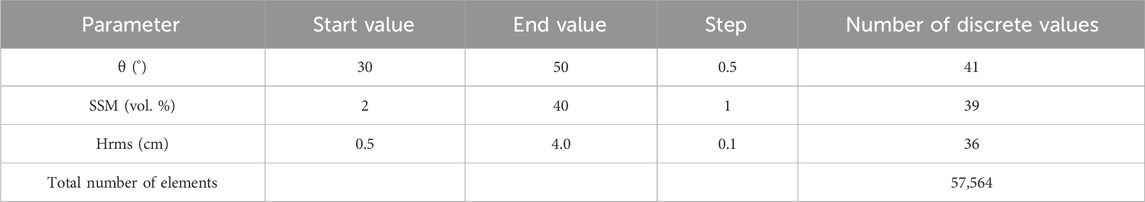
Table 1. Dubois-B input parameters used in this study.

The output of the Dubois-B model (simulated SAR data, σ⁰) is calculated from input parameters without any added noise. However, in real world use cases, SAR σ⁰ includes a certain amount of noise, depending on the radiometric accuracy of the instrument (Shimada et al., 2009; Motohka et al., 2018; Schmidt et al., 2020; Schwerdt et al., 2017). This radiometric error must be accounted for when employing simulated SAR data. For Sentinel-1, This error is approximately 0.70 dB (σ⁰) for co-polarizations (VV and HH) and 1.0 dB for cross polarization (HV) (Schwerdt et al., 2017). For ALOS281 2, this error is less than 0.8 dB, as shown by Motohka et al. (2018). The operational radiometric accuracy of NISAR is not yet known as the satellite data is not produced yet. For this reason, we will assume that NISAR will have a radiometric accuracy similar to other currently available SAR satellite mission (Sentinel-1 and ALOS-2). Therefore, a zero-mean Gaussian random noise with standard deviations of 0.7 dB (for VV and HH) and 1.0 dB (for HV) was introduced to synthetic σ⁰ for each element in our dataset (corresponding to a given θ, SSM, and Hrms). A hundred noise samples were randomly drawn for each element. These noise values (dB) were then added to the Dubois-B-simulated 288 σ⁰, generating 100 variations for each original element in our synthetic dataset. As a result, the noisy synthetic datasets were created for L- and S-bands, and in VV, HH, and HV polarizations, each containing 5,756,400 elements. This noisy synthetic data are supposed to approximate real NISAR data, assuming that real NISAR data will have similar radiometric accuracy to that of the noisy simulated datasets. Each point of the noisy synthetic dataset operationally represents the mean of backscattering coefficient over a spatially homogeneous unit (a plot or a mesh-cell) measuring a few hundred meters square. This will strongly reduce the effect of speckle excepted on real NISAR data because we are using the mean of pixels inside of a given spatial unit the influence of speckle noise will be reduced. For example, for a plot that is around 200 m × 200 m, the effect of speckle will be reduced by a factor of 20.

2.2 Neural network configurations

In this study, a NN approach was employed to estimate soil parameters from SAR data. The NNs were trained using the Levenberg–Marquardt algorithm (Marquardt, 1963) and structured with two hidden layers, each containing 20 neurons (Baghdadi et al., 2012) with Mean squared error (MSE) used as the loss function. This method was used because previous studies have shown that a network with two hidden layers and 20 neurons per layer provided accurate SSM estimates while maintaining reasonable computational efficiency (El Hajj et al., 2017). Both hidden layers employed a ReLU activation function (Schmidt-Hieber, 2020; Lin and Shen, 2018). Three SAR configurations were considered based on the polarimetric modes available for NISAR (Brancato and Fattahi, 2021), all three configurations utilized the L and S frequencies simultaneously:

• SP configuration: corresponds to the configuration where we use acquisitions from L- and S-bands in Single Polarization configuration. Noisy radar signal at HH polarization, and noisy radar signal at VV polarization were tested.

• DP configuration: corresponds to the configuration where we use acquisitions from L- and S-bands in Dual Polarization configuration: noisy radar signals at both HH and HV polarizations, as well as noisy radar signals at VV and VH polarizations were tested.

• QP configuration: corresponds to the configuration where we use acquisitions from L- and S-bands in Quad Polarization configuration noisy radar signal at HH, HV, and VV polarizations were used in input to inversion model.

NNs were trained using only θ and the noisy synthetic training backscattering coefficients generated from Dubois-B. Consequently, neither reference-SSM nor reference-Hrms were used as inputs for the estimation of soil parameters (SSM and Hrms) as these two are not known at the time of estimation. Furthermore, since NISAR operates the L- and S-bands in tandem, θ is the same for the two wavelengths employed (Rosen et al., 2017; Villano et al., 2018; Kellogg et al., 2020; NISAR, 2025). SSM and Hrms were estimated simultaneously using all three configurations.

Additionally, a priori information on natural soil moisture conditions was incorporated during NN training. Previous studies demonstrated that prior knowledge of soil moisture conditions significantly enhances estimation accuracy of SSM (Baghdadi et al., 2012; Hamze et al., 2021; El Hajj et al., 2017). Weather data, including precipitation and temperature from ERA5 reanalysis, in situ sensors, and remote sensing products like the Tropical Rainfall Measuring Mission (TRMM), can help indicate whether the soil is dry to slightly wet (after a prolonged dry period before SAR acquisition) or very wet (following heavy rainfall). By integrating this a priori information on SSM, the range of possible soil moisture estimates is constrained, improving both accuracy and mapping reliability in neural network models. For this reason, in addition to the NN built using the whole range of SSM (without a priori information on SSM), separate NNs are created for each of the two soil moisture state, one encompassing dry to slightly wet soil moisture conditions and one for very wet soil moisture conditions (with a priori information on SSM).

The impact of a priori information was assessed accordingly, NNs were trained with and without prior information on soil moisture. When splitting the noisy synthetic data to create a dataset for dry to slightly wet soils and another for the very wet soils, an overlap of 10 vol.% has been kept between the two training sub-datasets of the NNs. Here are the three developed cases (using both S- and L-bands):

• Case 1: No a priori information is used for the soil moisture state. In this case, the NN is trained using SSM between 2 and 40 vol.%.

• Case 2: With a priori information on soil moisture state. The soil is presupposed to be dry to slightly wet according to meteorological data (precipitation, temperature). The NN is trained using SSM between 2 and 30 vol.%.

• Case 3: With a priori information on soil moisture. The soil is presupposed to be very wet according to meteorological data (precipitation, temperature). The NN is trained using SSM between 20 and 40 vol.%.

When it comes to validation datasets, in the case without a priori information (case 1), the three NN configurations (SP, DP, and QP) were validated using the entire noisy validation dataset, with SSM values ranging from 2 to 40 vol.%. For the two cases with a priori information on SSM (cases 2 and 3), the NNs were validated using a dataset having SSM values ranging between 2 and 25 vol.% when the soil is assumed to be dry to slightly wet (case 2), and using a dataset having SSM values between 26 and 40 vol.%. in the case of very wet soil (case 3). Nine neural networks were developed for surface soil moisture and roughness estimation. Table 2 summarizes each developed neural network.

Table 2

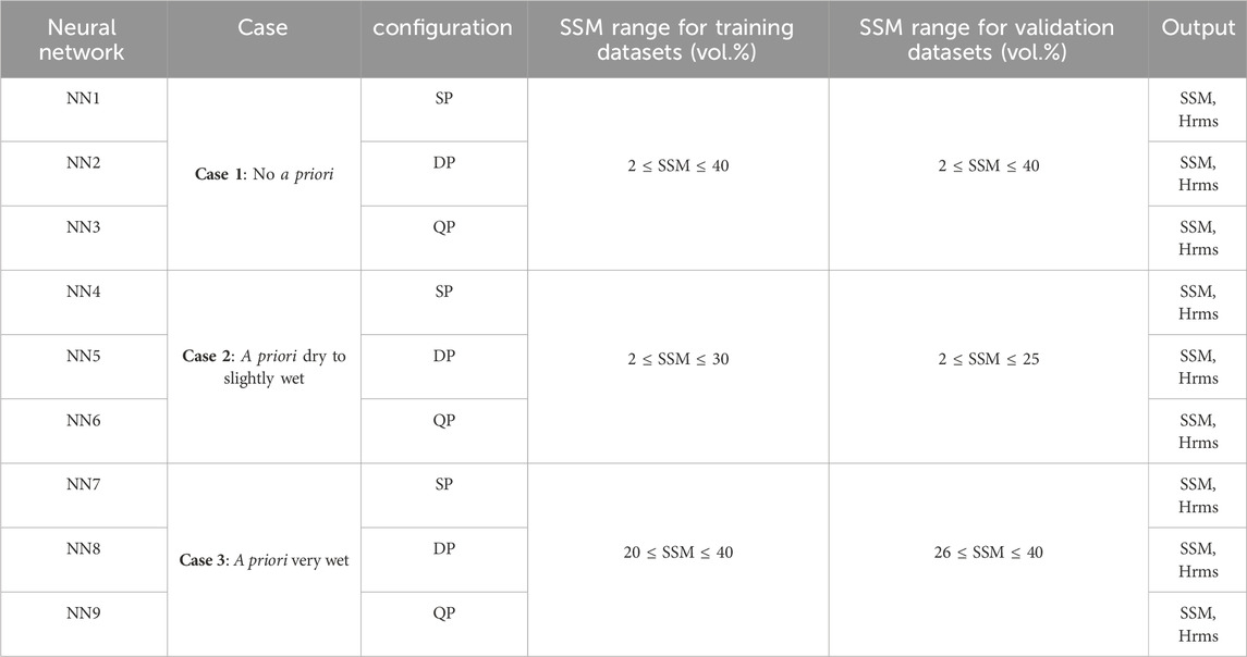
Table 2. Description of the NNs used in this study.

The performance analysis of each neural network was conducted on the noisy validation dataset that corresponds to each case (see Table 2). The estimated SSM and Hrms values from the neural networks are compared to the reference values (those used to simulate the SAR synthetic validation dataset), and the errors are quantified using Root Mean Square Error (RMSE) and bias (Estimated–Reference). Additionally, the RMSE and bias of SSM estimates are analyzed as a function of Hrms and θ values; while bias and RMSE of Hrms estimates were analyzed based on SSM and θ values.

3 Results

3.1 Estimated compared to reference SSM

The results of SSM estimation were analyzed first, by comparing estimated SSM to reference (input) SSM for each of the NNs (Figure 1).

Figure 1

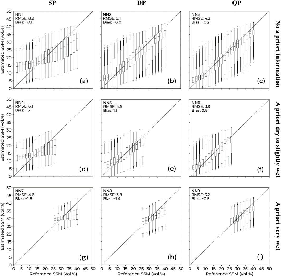
Figure 1. Estimated SSM as a function of reference SSM (a) NN1: single polarization (HH), no a priori information. (b) NN2: dual polarizations (HH and HV), no a priori information. (c) NN3: quad polarizations (HH, VV, and HV), no a priori information. (d) NN4: single polarization (HH), a priori dry to slightly wet. (e) NN5: dual polarizations (HH and HV), a priori dry to slightly wet. (f) NN6: quad polarizations (HH, VV, and HV), a priori dry to slightly wet. (g) NN7: single polarization (HH) a priori very wet. (h) NN8: dual polarizations (HH and HV), a priori very wet. (i) NN9: quad polarizations (HH, VV, and HV), a priori very wet. RMSE and bias are in vol.%.

Analysis of the results will be presented for each of the three cases: case 1: no a priori information, case 2: a priori dry to slightly wet, and case 3: a priori very wet. For single polarization NNs, the presented results correspond to HH polarization, as HH and VV exhibited similar performance. Results for VV are provided in the appendix (Supplementary Figures A7a, d, g). Likewise, results for DP configuration NNs using VV and VH instead of HH and HV can be found in the appendix (Supplementary Figures A7b, e, h). The similar soil moisture retrieval accuracy for HH and VV polarizations (difference of 0.2 vol.% without a priori soil moisture infomration) may be due to the fact that the sensitivity of the radar signal to soil moisture is not very dependent on polarization (e.g. (Sokol et al., 2004; Baghdadi et al., 2008)). A second possible explanation is that although some authors have shown a stronger sensitivity of the radar signal in HH (e.g. (Beaudoin et al., 1990)), this difference is not clearly visible in the simulated data.

Considering case 1, where we do not use a priori information, the NN developed using the single-polarization (SP) configuration (NN1) resulted in an RMSE of 8.2 vol.% (Figure 1a) compared to 5.1 vol.% for NN2 (Figure 1b), which uses dual-polarization (DP) configuration. Meanwhile, NN3 which utilizes quad-polarization (QP) configuration performed the best with an RMSE of 4.2 vol.% (Figure 1c). Furthermore, NN1 showed large over estimation of SSM for very low SSM values, and significant underestimation for high SSM values. Bias values were around 0 vol.% for all three NNs.

In case 2, where soil moisture conditions were assumed to be dry to slightly wet, the NN constructed using the SP configuration (NN4) showed an RMSE of 6.1 vol.% (Figure 1d), compared to 4.5 vol.% (Figure 1e) for NN5 (DP configuration); while NN6 (QP configuration) resulted in an RMSE of 3.9 vol.% (Figure 1f) which was the best out of the three. Similarly to case 1, the SP configuration (NN4) showed an important overestimation for low reference SSM and underestimation for high reference SSM. Bias was positive and varied from 1.5 vol.% for the SP configuration to 0.8 vol.% for the QP configuration.

Case 3 tells a similar story, NN9 (QP configuration) performed the best, with an RMSE of 3.2 vol.% (Figure 1g), followed by NN8 (DP configuration) with 3.8 vol.% (Figure 1h), and finally NN6 (SP configuration), with an RMSE of 4.6 vol.% (Figure 1i). There was no important overestimation at low SSM values, although we still have underestimation for high reference SSM values. Bias was negative ranging from −1.8 vol.% for the NN7, which uses SP configuration, to −0.5 vol.% for the NN using QP configuration.

Therefore, the quad-polarization configuration achieved the best SSM estimation, with errors consistently lower than the two other configurations tested (single-polarization and dual-polarization configurations). Furthermore, NNs constructed using a priori knowledge of soil moisture conditions performed better than NNs constructed without knowledge of soil moisture conditions, with improvements of RMSE. Estimated compared to reference Hrms.

Estimated Hrms were compared reference Hrms in Figure 2. When examining case 1 (without a priori knowledge of soil conditions), NN1 (Figure 2 using SP configuration) resulted in an RMSE of 0.7 cm (Figure 2a), while NN2 (using DP configuration) performs slightly better with an RMSE of 0.6 cm (Figure 2b), and NN3 (using QP configuration) performs the best estimations with an RMSE of 0.3 cm (Figure 2c). Bias was similar across the board at around 0.01 cm. For case 2 (a priori dry to slightly wet), NN4, which uses SP configuration, showed an RMSE of 0.6 cm (Figure 2d), while NN5 (Figure 2e, DP configuration) had an RMSE of 0.5 cm, and NN6, which uses the quad polarization, resulted in an RMSE of 0.3 (Figure 2f). NN4 and NN5 exhibited positive bias, with values of 0.15 and 0.06 cm, respectively, while NN6 showed no bias. For case 3 (a very wet) NN7, using the SP configuration, resulted in an RMSE of 0.5 cm (Figure 2g), RMSE was similar for NN8 (using DP configurations, Figure 2h), while NN9 (QP configuration) had an RMSE of 0.3 cm (Figure 2i). Bias was negative for the tested NNs, being highest for NN7 at −0.13 cm, followed by −0.07 cm for NN8 and −0.04 cm for NN9.

Figure 2

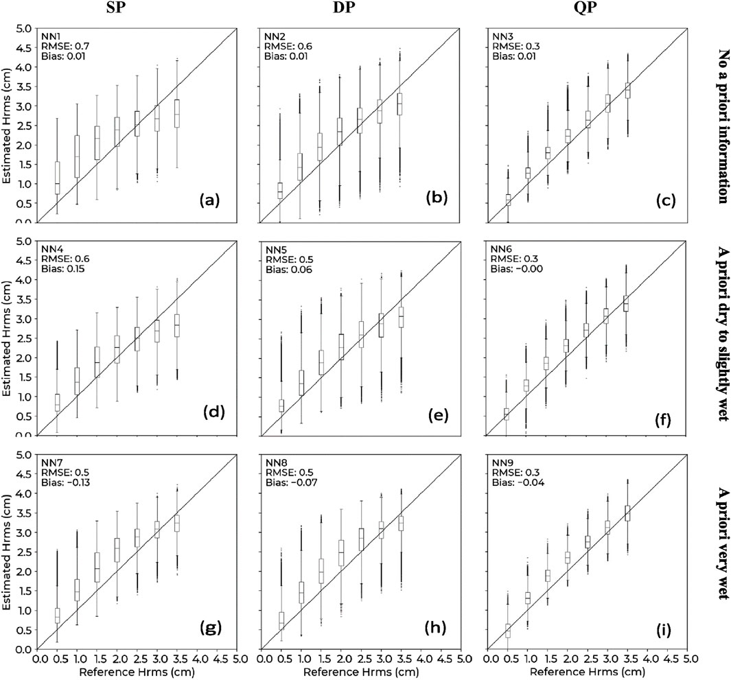
Figure 2. Estimated Hrms as a function of reference Hrms (a) NN1: single polarization (HH), no a priori information. (b) NN2: dual polarizations (HH and HV), no a priori information. (c) NN3: quad polarizations (HH, VV, and HV), no a priori information. (d) NN4: single polarization (HH), a priori dry to slightly wet. (e) NN5: dual polarizations (HH and HV), a priori dry to slightly wet. (f) NN6: quad polarizations (HH, VV, and HV), a priori dry to slightly wet. (g) NN7: single polarization (HH) a priori very wet. (h) NN8: dual polarizations (HH and HV), a priori very wet. (i) NN9: quad polarizations (HH, VV, and HV), a priori very wet. RMSE and bias are in cm.

Similar to SSM estimation, quad-polarization configuration performed the best Hrms estimation, with errors around half of the two other configurations (SP and DP configurations). Furthermore, the neural networks in our article output both soil moisture (SSM) and surface roughness (Hrms), and since the radar signal is related to both soil moisture and roughness, an improved estimation of SSM in the case of a priori information on SSM (thanks to the optimized estimation of soil moisture within a reduced range of SSM values) can lead to an improvement in Hrms estimation. This improvement is negligible for the QD configuration, which performs well in all three cases; however, we saw improvements between 0.1 and 0.2 cm for the SP and DP configurations (Figure 2).

3.2 Evaluating error in SSM estimation as a function of θ and Hrms

In this section, SSM estimation errors were analyzed using RMSE and bias metrics as a function of Hrms and θ values for each configuration in our study (SP, SP, and QP) and for each case (no a priori knowledge, a priori dry to slightly wet, a priori very wet). As in Section 3.1, for SP configuration, the NN tested utilized the HH polarization; results for VV are provided in the appendix (Supplementary Figures A8 and A9). Likewise, results for VV and VH instead of HH and HV can also be found in the appendix (Supplementary Figures A8 and A9).

Figure 3 shows the RMSE on SSM estimation as a function of θ and Hrms for the various NNs. For NNs constructed without a priori knowledge of soil moisture conditions, NN1 (SP configuration) had RMSE values ranging from around 6.0 vol.% for low θ values (30°), to around 9.5 vol.% for high θ values (50°). RMSE ranged from ∼3.5 to ∼6.0 vol.% for NN2 (DP configuration), and from ∼3.0 to ∼5.0 vol.% for NN3 (QP configuration). Figure 3b shows the effect of θ on RMSE when using a priori knowledge of dry to slightly wet soil conditions. RMSE ranged from ∼5.0 to ∼6.0 vol.% for NN4 (SP configuration), from ∼3.5 to ∼5.0 vol.% for NN5 (DP configuration), and from 2.8 to around 4 vol.% for NN6 (QP configuration). Figure 3c shows that RMSE ranged from ∼4.0 to ∼4.5 vol.%, for NN7 (SP configuration), from ∼3.0 to ∼4.0 vol.% for NN8 (DP configuration), and from ∼2.5 to ∼3.5 vol.% for NN9 (QP configuration). Therefore, RMSE increased as θ increased. Furthermore, incorporating a priori knowledge of soil moisture conditions, and using QP polarization reduced RMSE and narrowed its range as marked by the difference between the maximum and minimum RMSE (ΔRMSE) that was approximately 3.5 vol.% for NN1 and around 1.0 vol.% for NN9.

Figure 3

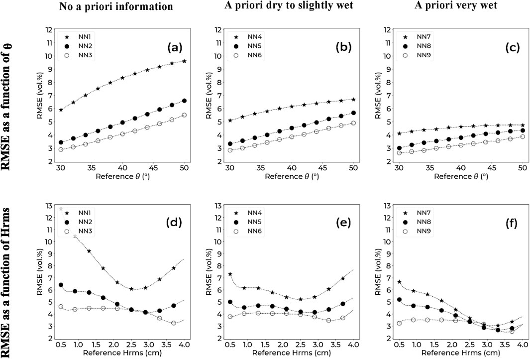
Figure 3. RMSE on SSM estimation as a function of reference θ (a–c) and as a function of reference Hrms (d–f) for each polarization-configuration. (a, d) No a priori information. (b, e) A priori dry to slightly wet. (c, f) A priori very wet. (NN1, NN4, NN7): single polarization (HH), (NN2, NN5, NN8):dual polarizations (HH and HV), (NN3, NN6, NN9): quad polarizations (HH, VV, and HV).

Figures 3d–f, show RMSE as a function of reference Hrms. For NNs constructed without a priori knowledge of SSM (Figure 3d), NN1 (SP configuration) had the highest RMSE for very high and very low Hrms values (∼13.0 vol.% at Hrms = 0.5 cm, and ∼9.0 vol.% at Hrms = 4.0 cm). NN2 (DP configuration) and NN3 (QP configuration) exhibited their highest RMSE values at ∼6.5 and ∼4.5 vol.%, respectively, for very low Hrms (0.5 cm). For NNs constructed for dry to slightly wet conditions (Figure 3e), RMSE for NN4 (SP) is highest for very low and very high Hrms values (∼7.0 vol.% for Hrms of 0.5 and 5.0 cm). For NN5 (DP) and NN6 (QP), RMSE values were around 4.5 and 4.0 vol.%, respectively across the range of Hrms. For NNs developed for very wet conditions, NN7 (SP configuration) and NN8 (DP configuration) had their highest RMSE values for very low Hrms (∼6.5 and ∼5.0 vol.% for Hrms = 0.5 cm) while NN9 (QP configuration) resulted in an RMSE of around 3.5 vol.% across the range of Hrms values.

RMSE was highest at both the lowest and highest Hrms values in our study, particularly when using the SP configuration. However, using the QP configuration and a priori knowledge of soil moisture conditions significantly reduced RMSE and minimized the impact of Hrms on SSM estimation.

Figure 4 presents the bias on SSM estimation as a function of θ and Hrms for the various NNs. Figure 4a shows that without a priori knowledge of soil moisture conditions, Bias is around 0 vol.% for NN1, NN2, and NN3 (no bias). In the case of a priori dry to slightly wet conditions, bias was positive, NN4 (SP configuration) had a bias ranging from 1.0 for low θ (30°) to 2.0 for high θ (50°). For NN5 (DP configuration), bias ranged between 0.5 and 2.0 vol.%, and NN6 (QP configuration) ranged between 0.5 and 1.0 vol.% (Figure 4b). When working in very wet soil moisture conditions (Figure 4c), bias that more negative greater when θ increases, ranging from −1.0 to −2.0 vol.%, for NN7 (SP configuration), from ∼−0.5 to ∼−1.5 vol.% for NN8 (DP configuration), and from ∼0 to ∼−1 vol.% for NN9 (QP configuration).

Figure 4

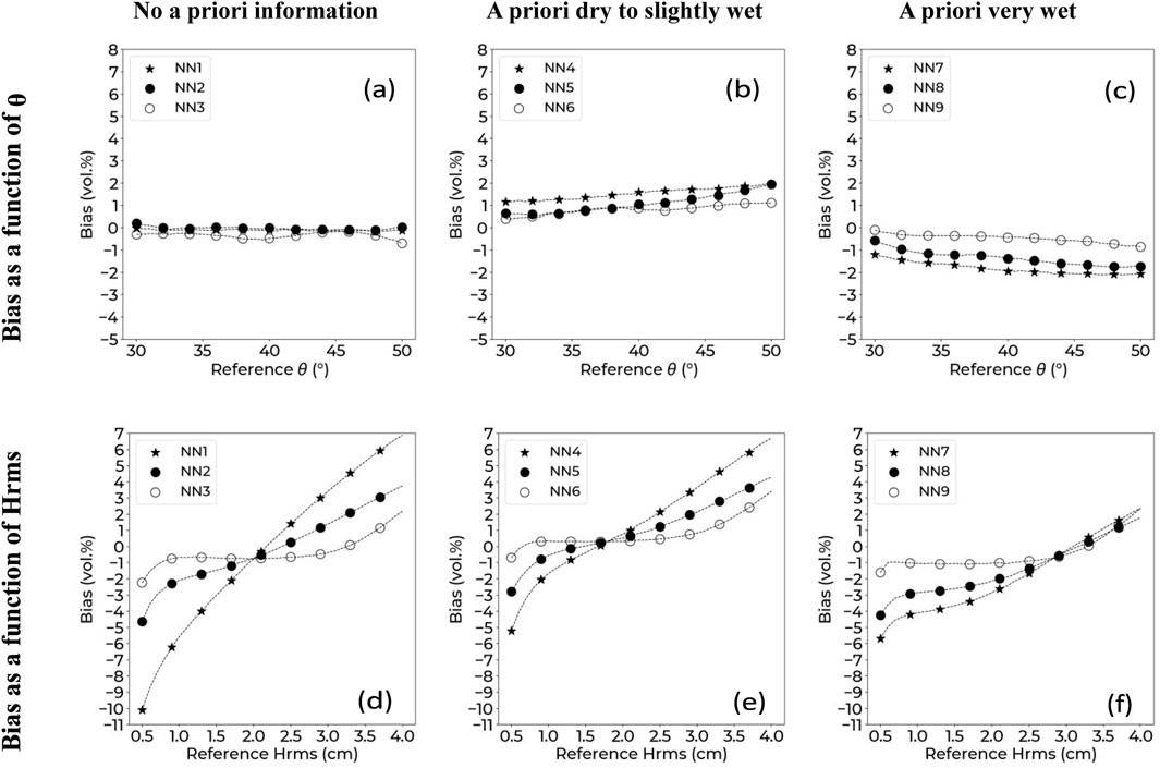
Figure 4. Bias on SSM estimation as a function of reference θ (a–c) and as a function of reference Hrms (d–f) for each polarization-configuration. (a, d) No a priori information. (b, e) A priori dry to slightly wet. (c, f) A priori very wet. (NN1, NN4, NN7): single polarization (HH), (NN2, NN5, NN8): dual polarizations (HH and HV), (NN3, NN6, NN9): quad polarizations (HH, VV, and HV).

Figures 4d–f show estimation bias as a function of reference Hrms. When a priori soil condition knowledge was not used, bias values ranged from −10.0 to 7.0 vol.%, when Hrms increased from 0.5 to 4.0 cm, for NN1 (SP configuration), from −5.0 to 3.5 vol.% for NN2 (DP configuration) and from −2.0 to 3.0 vol.% for NN3 (SP configuration) (Figure 4d). NNs constructed for a priori dry to slightly wet conditions resulted in smaller ranges of bias values, with NN4 resulting in bias values varying between −5.0 to 6.5 vol.%, as Hrms increased from 0.5 to 4.0 cm NN5 resulted in bias values ranging from −3.0 to 4.0 vol.%, while bias values for NN6 ranged from −1.0 to 3.0 vol.%. For NNs constructed with a priori knowledge of very wet soil moisture conditions, bias values ranged from −6.0 to 2.0 vol.% and from −4.0 to 2.0 vol.%, respectively for NN7 (SP configuration) and NN8 (DP configuration) when Hrms increases from 0.5 to 4.0 cm NN9 (QP configuration) shows a mostly constant bias at around −1.0 vol.% for Hrms values between 0.5 and 3.0 cm, outside that range, bias increases, reaching 2.0 vol.% for Hrms of 4.0 cm.

Bias was generally more negative for lower Hrms values and more positive for higher Hrms values. However, the effect of Hrms on bias was reduced when using QP configuration and a priori knowledge of soil moisture conditions, as shown by the improvement in the range of bias between NN1 and NN9, as Δbias was ∼17.0 vol.% for NN1 and ∼2.0 vol.% for NN9.

3.3 Evaluating error in Hrms estimation as a function of θ and SSM

In this section, Hrms estimation were assessed using RMSE and bias values as a function of reference SSM and θ values for each configuration in our study (SP, SP, and QP). RMSE has been calculated without a priori knowledge of soil moisture conditions because the results of Section 3.2 showed that using a priori knowledge did not significantly enhance Hrms estimation. Figure 5a shows the RMSE on Hrms estimation as a function of reference θ. For NN1 (SP configuration), RMSE values decreased from ∼0.9 to ∼0.6 cm when θ increases from 30° to 50°. For NN2 (DP configuration), RMSE went from ∼0.7 down to ∼0.5 cm when θ increases, while for NN3 (QP configuration), RMSE values decreased from ∼0.4 to ∼0.3 cm when θ decreased. ΔRMSE, calculated as the difference between maxRMSE and minRMSE, was ∼0.3 cm for NN1, compared to ∼0.2 cm for NN2, and ∼0.1 cm for NN3, which had the lowest RMSE values overall. Figure 5b shows RMSE as a function of reference SSM. NN1 had its highest RMSE at around 1.0 cm for very low and very high SSM reference SSM values (2 vol.%, and 40 vol.%, respectively). The lowest RMSE achieved by NN1 was around 0.6 cm for an SSM value of around 20 vol.%, NN2 showed RMSE varying between ∼0.5 and ∼0.6 cm, while NN3 had the lowest overall RMSE varying between ∼0.3 and ∼0.4 cm.

Figure 5

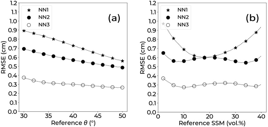
Figure 5. RMSE on Hrms estimation as a function of reference θ (a) and as a function of reference SSM (b). NN1: SP configuration (HH), NN2: DP configuration (HH and HV), NN3. QP configuration (HH, VV, and HV).

Therefore, RMSE decreased when θ increases. Moreover, RMSE was highest for very low and very high SSM values. However, for the QP configuration (NN3), these effects were not as strong when compared to the other polarization-configurations.

Figure 6a presents the bias values as a function of reference θ. Bias was around 0 cm for the three NNs tested with NN3 having slight positive bias of around 0.1 cm for really high and really low θ values (30° and 50°, respectively). The bias was also examined as a function of reference SSM (Figure 6b). For NN1 (SP configuration), there was a negative bias for low SSM values (lower than 20 vol.%), reaching −0.8 cm at an SSM of 2.0 vol.%. Conversely, for high SSM values (>20 vol.%), the bias was positive, reaching 0.8 cm at an SSM of 40 vol.%. Similarly, for NN2 (DP configuration) and NN3 (QP configuration), the bias followed the same trend: negative for low SSM values and positive for high SSM values. For NN2, the bias reached −0.4 cm at an SSM of 2.0 vol.% and 0.4 cm at 40 vol.%. For NN3, the bias was the smallest, reaching −0.2 cm at 2.0 vol.% and 0.2 cm at 40 vol.%.

Figure 6

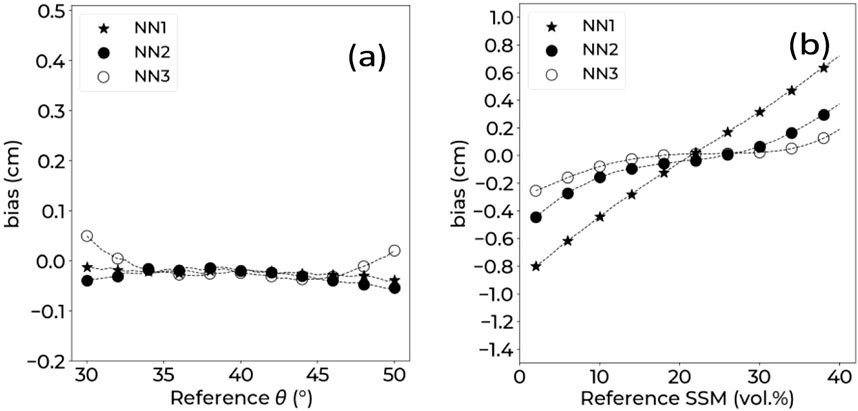
Figure 6. RMSE on Hrms estimation as a function of reference θ (a) and as a function of reference SSM (b). NN1: SP configuration (HH), NN2: DP configuration (HH and HV), NN3. QP configuration (HH, VV, and HV).

4 Discussion

A noisy synthetic SAR dataset of S and L frequency bands was created following Dubois-B simulations of SAR backscattering coefficients. This dataset was then split equally into a training dataset, and validation dataset with the aim to estimate both the surface soil moisture (SSM) and the surface roughness (Hrms) using neural networks. Validation was carried out using synthetic data only because NISAR data is not yet operational and so the data is not yet available (launch expected in 2025). NISAR will provide L- and S-bands acquisitions simultaneously in three configurations: Single-, Dual-, and Quad-Polarization configurations. These configurations were tested without a priori information on soil moisture conditions, and with a priori information on the soil moisture conditions (dry to slightly wet or very wet soils). Results showed that the quad polarization configuration achieved the highest precision for SSM and Hrms estimation, performing better than single and dual polarizations configurations.

4.1 Analysis of estimation errors

Errors in SSM estimates from neural networks were shown to be influenced by SAR incidence angle (θ) and by soil surface roughness (Hrms). Regarding the effect of incidence angle, RMSE on SSM was highest when θ was highest for all NNs tested, however QP configuration proved to be less affected by θ when compared to other configurations. This degradation in SSM estimation with increasing radar incidence is well documented in the literature, as the sensitivity of the radar signal to soil moisture decreases with increasing incidence angle due to noise caused by soil roughness (Aubert et al., 2011; Baghdadi et al., 2008).

Additionally, for NNs constructed with a priori knowledge of dry to slightly wet soil moisture conditions, there was a slight overestimation (positive estimation bias) that gently increased when θ increases. Inversely, for NNS constructed with a priori very wet soil moisture conditions, a slight underestimation (negative estimation bias) was observed, slightly increasing when θ increases. This underestimation of SSM for high moisture values (30–40 vol.%) is due to saturation of the radar signal for this range of SSM (30–40 vol.%) (Baghdadi et al., 2016).

Regarding the effect of Hrms on SSM estimation, when no a priori information on SSM was used, very low or very high Hrms led to an increase in RMSE for SP configuration. For DP configuration, RMSE on SSM decreased when Hrms decreased; while QP configuration was not significantly affected by Hrms. For a priori dry to slightly wet condition, RMSE on SSM for SP configuration was highest for very low or very high Hrms, while Hrms did not affect RMSE on SSM for the DP and QP configurations in this soil moisture condition. Regarding a priori very wet conditions, RMSE on SSM for the SP and DP configurations increased when Hrms decreases, while Hrms did not significantly affect RMSE of the QP configuration. Regarding bias, lower Hrms values led to more negative SSM estimation bias while higher Hrms values led to more positive SSM estimation bias for all cases, with QP configuration performing the best being affected less than SP and DP configurations by Hrms. These over- and under-estimation of the SSM estimates depending on the range of Hrms were observed by El Hajj et al. (2017), who note that a smooth surface (Hrms < 1 cm) results in decreased backscattering and underestimated SSM with high RMSE on SSM. On the other hand, a rough surface (Hrms > 3.0 cm) augments radar backscatter, leading to SSM overestimation. However, NNs using the Quad polarization configuration were able to mitigate this limitation of smooth or rough surfaces.

Regarding Hrms estimation errors, RMSE on Hrms was shown to be affected by θ for both SP and DP configurations, as RMSE decreases when θ increases. This better estimation of ground roughness for high values of θ is due to a better sensitivity of the radar signal to roughness for high values of θ compared to low incidence angles values because the dependence of the radar signal on surface roughness in agricultural areas is mainly significant at high incidence angles (Baghdadi et al., 2008). Hrms estimated from QP configuration was not shown to be affected by θ. SSM affected Hrms estimation errors for very high and for very low SSM, when using SP configuration, however there was no significant effect for neither the DP or QP configurations. On the other hand, SSM affected bias for Hrms estimation with negative bias for low SSM value and positive bias for high SSM values with QP configuration being affected less than the SP and QP configuration.

4.2 Using a priori knowledge of soil moisture conditions

In this study, three cases were examined 1) no a priori knowledge of soil moisture conditions, 2) soil conditions were considered known as dry to slightly wet, 3) soil conditions were considered known as very wet. Incorporating a priori information that can be easily obtained from in situ precipitation stations or from other sources (remote sensing data or/and model-based simulation) enhances the precision of SSM estimates. However, in the cases where soil moisture conditions is known, the range of SSM values in the training phase are smaller (case 2: 2 vol.% ≤ SSM ≤ 30 vol.%; case 3: 20 vol.% ≤ SSM ≤ 40 vol.%) compared to the range of SSM values when no a priori soil moisture knowledge were used (case 1: 2 vol.% ≤ SSM ≤ 40 vol.%), reducing the over- and underestimations of SSM. Therefore, in order to correctly assess the improvement in SSM estimation in the cases of a priori information on SSM, the same range of SSM has be considered when calculating RMSE on SSM estimates. Table 3 shows RMSE and Bia values on SSM estimation when using the same range of SSM values for NN constructed without and with a priori information of soil moisture conditions. When comparing NNs for without a priori knowledge of soil moisture condition (case1: NN1, NN4, and NN7) to NNs constructed with a priori knowledge of dry to slightly wet conditions (case 2: NN2, NN5, and NN8), RMSE was calculated using only SSM values ranging between 2 and 25, which is the range used for a priori dry to slightly wet NNs. Similarly, when comparing non a priori NNs to NNs constructed with a priori knowledge of very wet conditions (case 3: NN3, NN6, and NN9), RMSE was calculated using only SSM values ranging between 26 and 40, which is the range used for a priory very wet NNs. Table 3 shows that the improvement in RMSE on SSM for a priori dry to slightly wet NNs in “non a priori” NNs was 1.2 vol.% for SP configuration, 0.5 vol.% for DP configuration, and 0.3 for QP configuration. For “a priori very wet” NNs, the improvement in RMSE was 3.6 vol.% for SP configuration, 1.4 vol.% for DP configuration, and 1.0 vol.% for QP configuration. Therefore, using a priori knowledge of soil moisture conditions slightly improved the SSM estimation results when working in dry to slightly wet soil conditions, and greatly improved soil moisture estimation when working in very wet soil condition for all NISAR configurations.

Table 3

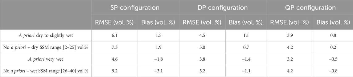
Table 3. Performance on SSM estimates of a priori NNs compared to no a priori NNs.

4.3 Using single frequency data (L or S-band)

NISAR will provide both of S and L frequency bands simultaneously, enabling dual-frequency radar observations during a single pass (NISAR, 2025; Kellogg et al., 2020). This is a significant feature of NISAR, not currently available in other SAR constellations. For this reason, our work used L and Sbands in tandem; however, it is important to assess the use of two frequency bands by comparing it to results we get using a single frequency band.

For this reason, single-frequency noisy datasets were built for each frequency band (L, and S-band). For each of these two, NNs were constructed and tested in the Single, Dual, and Quad-polarization configurations. Table 4 compares RMSE values for SSM estimation resulting from NN built using two frequencies and one frequency and without a priori knowledge of soil moisture condition (the entire range of SSM). L-band and S-band showed similar performance showed in the table as “L or S-band.” As seen in Table 4, NNs utilizing both L- and S-bands together consistently outperformed those relying on a single band, achieving lower RMSE values across all configurations. Specifically, in the SP configuration, RMSE increased from 8.2 vol.% (dual frequency bands) to 9.3 vol.% (single frequency band), reflecting a 1.1 vol.% performance degradation when using only one frequency. Similarly, in the DP configuration, RMSE increased from 5.1 vol.% (dual frequency band) to 6.2 vol.% (single frequency band), and in the QP configuration, it worsened from 4.2 vol.% to 5.4 vol.%, indicating a 1.2 vol.% decline. These findings underscore the benefits of dual-frequency SAR observations, which provide more accurate soil moisture estimates by integrating complementary scattering information from both frequency bands.

Table 4

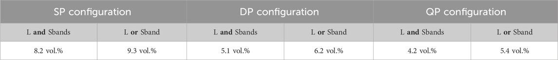
Table 4. Comparing RMSE values (vol.%) on SSM estimates for of Dual and Single frequency bands, without a priori knowledge of soil moisture conditions.

Table 5 compares RMSE values for Hrms estimation (cm) without a priori knowledge of soil moisture condition using both L and S bands or one of the bands only (L or S). NNs utilizing both L- and Sbands together performed better than NNs relying on a single band, achieving lower RMSE of around 0.1 cm across the different configurations.

Table 5

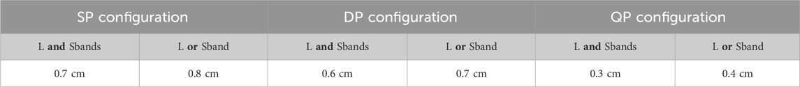
Table 5. Comparing RMSE values (cm) on Hrms estimates, for of Dual and Single frequency bands, without a priori knowledge of soil moisture conditions.

4.4 Comparison with L-band alone and with Sentinel-1 C-band SAR

In order to better assess the use of multiple frequencies simultaneously for soil moisture estimation, results of the dual frequency (L- and S-band) bands were compared to single frequency (L-band). When working without a priori information on SSM, using L-band alone (results not presented in the manuscript), achieved an RMSE on SSM estimation of 8.3 vol.% for SP configuration, 6.1 vol.% for the DP configuration and 5.3 vol.% for the QP configuration. Therefore, using dual frequency bands results in better SSM estimation of around 0.2 vol.% for the SP configuration, 1.0 vol.% for the DP configuration and around 1.1 vol.% for the QP configuration. NISAR Soil Moisture Science Team (2023) also investigated the benefit of using the dual frequency bands compared to L-band only, utilizing only the single polarization configuration (HH only) with results of dual-frequencies showing improvements in unbiased RMSE of 1 vol.% for corn and 0.2 vol.% for soybean over single frequency (L-band).

Concerning Sentinel-1, the S1 constellation currently provides satellite acquisitions in cross polarization configuration (VV/VH) over the majority of the Globe (P. Potin et al., 2019; Ticehurst et al., 2019). It is one of the more widely used SAR constellation for SSM and Hrms estmation (Hamze et al., 2021; Choker et al., 2017; El Hajj et al., 2017; Choker, Baghdadi, and Zribi, 2018). In recent works, (Ettalbi et al., 2023), constructed NN model trained and validated using synthetic C-band data simulated using the Integral Equation Model (IEM) model. In the validation phase using synthetic dataset, they showed that the Dual-polarization (VV and VH) lead to RMSE on SSM of around 6.0 vol.%. In addition, Choker, Baghdadi, and Zribi (2018) applied NNs, trained with synthetic data, on S1 data for SSM and Hrms estimation, with dual polarization performing better than single polarization, resulting in an SSM estimation with a RMSE of 7.5 vol.% and 5.8 vol.% when using NNs constructed without, and with a priori knowledge of soil moisture conditions, respectively. Regarding Hrms estimation, Choker et al. (2018) obtained an RMSE of 0.8 cm when working without a priori knowledge of soil moisture conditions and 0.7 cm when working with a priori knowledge of soil moisture conditions.

Compared to these findings by Ettalbi et al. (2023), and Choker et al. (2018), the NNs developed in our work performed better, resulting in lower RMSE values when using the DP and QP configurations. A few reasons are behind this improvement. Firstly, Sentinel-1 operates at a single frequency (C-band, wavelength ∼ 5 cm) whereas NISAR can rely on two bands (L and S-bands); these two independent frequency bands could provide complementary information that improve to performance of the NNS. Secondly, Sentinel-1 operates in the cross polarization mode (VV/VH), meaning that it is limited to using NNs in the DP configuration whereas NISAR can provide quadpolarization data. What is notable here is that in our work, the DP configuration was significantly outperformed by the QP configuration in terms of overall error as well as in terms of performance stability thus signaling the potential importance of NISAR for SSM and Hrms estimation.

5 Conclusion

This study aims to gauge the potential of using data from the NISAR satellite for SSM and Hrms estimation over bare soils. The NISAR satellite will utilize L and S frequency bands and will provide data in single-, dual-, and quad-polarization configurations. For this reason, simulated radar backscattering coefficients in NISAR configurations were generated for S- and L-bands using the Dubois-B model. Using S- and L-bands data simultaneously, nine neural networks were constructed, assessing each of NISAR’s three polarization configurations (single “SP”, dual “DP” and quad “QP” polarization). Additionally, a priori information on soil moisture conditions, that could be obtained using meteorological data, was tested (no a priori, a priori dry to slightly wet soils, and a priori very wet soils).

Results showed that without a prior information on soil moisture, RMSE on SSM estimation is 4.2 vol.% for the QP configuration, compared to 5.1 vol.% and 8.2 vol.% for the SP and DP configurations, respectively. Similarly, the RMSE for Hrms was 0.3 cm in the QP configuration, whereas it increased to 0.7 and 0.6 cm in the SP and DP configurations, respectively. Therefore, quad-polarization (QP configuration) is the most performant for SSM and Hrms estimation. Furthermore, the QP configuration reduced the impact of the SAR incidence angle (θ) and the Hrms on the SSM estimates, exhibiting RMSE values consistently lower than those of single-polarization (SP) and dual-polarization (DP) configurations across the range of θ. Comparing the use of dual-frequency and single-frequency showed that using both S- and L-bands improves SSM and Hrms estimation compared to using either S- or L-band alone. Additionally, our study found that using a priori knowledge of soil moisture conditions improves SSM estimation precision for all NISAR configurations, especially for very wet soil moisture conditions, but has little impact on Hrms estimation.

These results highlight the potential of future NISAR data for SSM and Hrms estimation and lay the groundwork for applying NNs trained on synthetic data (from radar backscattering models). Future work will focus on validating these NNs using real NISAR data, comparing estimates to in situ SSM and Hrms measurements.

Future works would focus on building NISAR data inversion networks over agricultural surfaces with vegetation cover. This requires the use of a radar backscatter model integrating soil and vegetation components. One of the most frequently used models is the Water Cloud Model, which can be calibrated using real NISAR backscatter coefficient data in conjunction with in situ moisture and roughness measurements. The vegetation component is in general modeled using a vegetation index calculated from optical images (Sentnel-2, Landsat, among others). Furthermore, in this approach, we trained neural networks which, would rely solely on imagery-derived data, when real data become available. However, machine learning methods usually benefit from more input features (e.g., environmental, meteorological), improving retrieval accuracy. Indeed, Auxiliary data sometimes used in addition to radar and optical data sources (air temperature, precipitation, net radiation, digital elevation model, soil texture…) could provide significant added value.

Data availability statement

The raw data supporting the conclusion of this article will be made available by the authors, without undue reservation.

Author contributions

SN: Conceptualization, Data curation, Formal Analysis, Investigation, Methodology, Project administration, Software, Supervision, Validation, Visualization, Writing – original draft, Writing – review and editing. NB: Conceptualization, Formal Analysis, Funding acquisition, Methodology, Project administration, Resources, Supervision, Validation, Writing – review and editing. HB: Formal Analysis, Methodology, Supervision, Validation, Writing – review and editing. MZ: Validation, Writing – review and editing. DP: Validation, Writing – review and editing. MS: Validation, Writing – review and editing.

Funding

The author(s) declare that financial support was received for the research and/or publication of this article. This research received funding from the National Research Institute for Agriculture, Food and the Environment (INRAE), and from the French Space Study Center (CNES, TOSCA 2024-2025 project).

Acknowledgments

The authors wish to thank the National Research Institute for Agriculture, Food and the Environment (INRAE), and the French Space Study Center (CNES, TOSCA 2024-2025) for supporting this work.

Conflict of interest

The authors declare that the research was conducted in the absence of any commercial or financial relationships that could be construed as a potential conflict of interest.

The author(s) declared that they were an editorial board member of Frontiers, at the time of submission. This had no impact on the peer review process and the final decision.

Generative AI statement

The author(s) declare that no Generative AI was used in the creation of this manuscript.

Publisher’s note

All claims expressed in this article are solely those of the authors and do not necessarily represent those of their affiliated organizations, or those of the publisher, the editors and the reviewers. Any product that may be evaluated in this article, or claim that may be made by its manufacturer, is not guaranteed or endorsed by the publisher.

References

Acutis, M., and Donatelli, M. (2003). SOILPAR 2.00: software to estimate soil hydrological parameters and functions. Eur. J. Agron. 18 (3), 187–393. doi:10.1016/S11610301(02)00128-4

CrossRef Full Text | Google Scholar

Attema, E. P. W., and Ulaby, F. T. (1978). Vegetation modeled as a water Cloud. Radio Sci. 13 (2), 357–364. doi:10.1029/RS013i002p00357

CrossRef Full Text | Google Scholar

Aubert, M., Baghdadi, N., Zribi, M., Douaoui, A., Loumagne, C., Baup, F., et al. (2011). Analysis of TerraSAR-X data sensitivity to bare soil moisture, roughness, composition and soil crust. Remote Sens. Environ. 115 (8), 1801–1810. doi:10.1016/j.rse.2011.02.021

CrossRef Full Text | Google Scholar

Aubert, M., Baghdadi, N. N., Zribi, M., Ose, K., El Hajj, M., Vaudour, E., et al. (2013). Toward an operational bare soil moisture mapping using TerraSAR-X data acquired over agricultural areas. IEEE J. Sel. Top. Appl. Earth Observations Remote Sens. 6 (2), 900–916. doi:10.1109/JSTARS.2012.2220124

CrossRef Full Text | Google Scholar

Baghdadi, N., Cerdan, O., Zribi, M., Auzet, V., Darboux, F., El Hajj, M., et al. (2008). Operational performance of current synthetic aperture radar sensors in mapping soil surface characteristics in agricultural environments: application to hydrological and erosion modelling. Hydrol. Process. 22 (1), 9–20. doi:10.1002/hyp.6609

CrossRef Full Text | Google Scholar

Baghdadi, N., Choker, M., Zribi, M., El Hajj, M., Paloscia, S., Verhoest, N. E. C., et al. (2016). A new empirical model for radar scattering from bare soil surfaces. Remote Sens. 8 (11), 920. doi:10.3390/rs8110920

CrossRef Full Text | Google Scholar

Baghdadi, N., Cresson, R., El Hajj, M., Ludwig, R., and La Jeunesse, I. (2012). Estimation of soil parameters over bare agriculture areas from C-band polarimetric SAR data using neural networks. Hydrology Earth Syst. Sci. 16 (6), 1607–1621. doi:10.5194/hess-161607-2012

CrossRef Full Text | Google Scholar

Baghdadi, N., Holah, N., and Zribi, M. (2006). Soil moisture estimation using multi-incidence and multi-polarization ASAR data. Int. J. Remote Sens. 27 (10), 1907–1920. doi:10.1080/01431160500239032

CrossRef Full Text | Google Scholar

Baghdadi, N., and Zribi, M. (2016). “Characterization of soil surface properties using radar remote sensing,” in Land surface remote sensing in continental hydrology. Editors N. Baghdadi, and M. Zribi (Elsevier), 1–39. doi:10.1016/B978-1-78548-1048.50001-2

CrossRef Full Text | Google Scholar

Baghdadi, N., Zribi, M., Paloscia, S., Verhoest, N. E. C., Mattia, F., Baup, F., et al. (2015). Semi-empirical calibration of the integral equation model for Co-polarized L-band backscattering. Remote Sens. 7 (10), 13626–13640. doi:10.3390/rs71013626

CrossRef Full Text | Google Scholar

Bazzi, H., Baghdadi, N., Charron, F., and Zribi, M. (2022). Comparative analysis of the sensitivity of SAR data in C and L bands for the detection of irrigation events. Remote Sens. 14 (10), 2312. doi:10.3390/rs14102312

CrossRef Full Text | Google Scholar

Beaudoin, A., Le Toan, T., and Gwyn, Q. H. J. (1990). SAR observations and modeling of the C-band backscatter variability due to multiscale geometry and soil moisture. IEEE Trans. Geoscience Remote Sens. 28 (5), 886–895. doi:10.1109/36.58978

CrossRef Full Text | Google Scholar

Brancato, V., and Fattahi, H. (2021). UAVSAR observations of InSAR polarimetric phase diversity: implications for NISAR ionospheric phase estimation. Earth Space Sci. 8 (4), e2020EA001445. doi:10.1029/2020EA001445

CrossRef Full Text | Google Scholar

Camillo, P. J., Gurney, R. J., and Schmugge, T. J. (1983). A soil and atmospheric boundary layer model for evapotranspiration and soil moisture studies. Water Resour. Res. 19 (2), 371–380. doi:10.1029/WR019i002p00371

CrossRef Full Text | Google Scholar

Chen, K. S., Wu, T.-D., Tsang, L., Li, Q., Shi, J., and Fung, A. K. (2003). Emission of rough surfaces calculated by the integral equation method with comparison to three-dimensional moment method simulations. IEEE Trans. Geoscience Remote Sens. 41 (1), 90–101. doi:10.1109/TGRS.2002.807587

CrossRef Full Text | Google Scholar

Choker, M., Baghdadi, N., and Zribi, M. (2018). Estimation of Surface Roughness over Bare Agricultural Soil from Sentinel-1 Data, Estimation de La Rugosité Du Sol En Milieux Agricoles à Partir de Données Sentinel-1. AgroParisTech. Available online at: https://theses.hal.science/tel-02293194.

Google Scholar

Choker, M., Baghdadi, N., Zribi, M., El Hajj, M., Paloscia, S., Verhoest, N. E. C., et al. (2017). Evaluation of the Oh, Dubois and IEM backscatter models using a large dataset of SAR data and experimental soil measurements. Water 9 (1), 38. doi:10.3390/w9010038

CrossRef Full Text | Google Scholar

Colliander, A., Reichle, R. H., Crow, W. T., Cosh, M. H., Chen, F., Chan, S., et al. (2022). Validation of soil moisture data products from the NASA SMAP mission. IEEE J. Sel. Top. Appl. Earth Observations Remote Sens. 15, 364–392. doi:10.1109/JSTARS.2021.3124743

CrossRef Full Text | Google Scholar

Das, N. N., Entekhabi, D., Scott Dunbar, R., Colliander, A., Chen, F., Crow, W., et al. (2018). The SMAP mission combined active-passive soil moisture product at 9 km and 3 km spatial resolutions. Remote Sens. Environ. 211 (June), 204–217. doi:10.1016/j.rse.2018.04.011

CrossRef Full Text | Google Scholar

Dinesh, D., Kumar, S., and Saran, S. (2024). Machine learning modelling for soil moisture retrieval from simulated NASA-ISRO SAR (NISAR) L-band data. Remote Sens. 16 (18), 3539. doi:10.3390/rs16183539

CrossRef Full Text | Google Scholar

Du, S., Duan, P., Zhao, T., Wang, Z., Niu, S., Ma, C., et al. (2024). An improved Change detection method for high-resolution soil moisture mapping in permafrost regions. GIScience Remote Sens. 61 (1), 2310898. doi:10.1080/15481603.2024.2310898

CrossRef Full Text | Google Scholar

Dubois, P. C., and Van Zyl, J. (1994). An empirical soil moisture estimation algorithm using imaging radar. Proc. IGARSS ’94 - 1994 IEEE Int. Geoscience Remote Sens. Symposium 3, 1573–1575. doi:10.1109/IGARSS.1994.399501

CrossRef Full Text | Google Scholar

Dubois, P. C., van Zyl, J., and Engman, T. (1995). Measuring soil moisture with imaging radars. IEEE Trans. Geoscience Remote Sens. 33 (4), 915–926. doi:10.1109/36.406677

CrossRef Full Text | Google Scholar

El Hajj, M., Baghdadi, N., Bazzi, H., and Zribi, M. (2019). Penetration analysis of SAR signals in the C and L bands for wheat, maize, and grasslands. Remote Sens. 11 (1), 31. doi:10.3390/rs11010031

CrossRef Full Text | Google Scholar

El Hajj, M., Baghdadi, N., Zribi, M., and Bazzi, H. (2017). Synergic use of sentinel-1 and sentinel-2 images for operational soil moisture mapping at high spatial resolution over agricultural areas. Remote Sens. 9 (12), 1292. doi:10.3390/rs9121292

CrossRef Full Text | Google Scholar

El Hajj, M., Baghdadi, N., Zribi, M., Belaud, G., Cheviron, B., François, C., et al. (2016). Soil moisture retrieval over irrigated grassland using XBand SAR data. Remote Sens. Environ. 176 (April), 202–218. doi:10.1016/j.rse.2016.01.027

CrossRef Full Text | Google Scholar

Engman, E. T. (1991). Applications of microwave remote sensing of soil moisture for water resources and agriculture. Remote Sens. Environ. 35 (2), 213–226. doi:10.1016/0034-4257(91)90013-V

CrossRef Full Text | Google Scholar

Ettalbi, M., Baghdadi, N., Garambois, P.-A., Bazzi, H., Ferreira, E., and Zribi, M. (2023). Soil moisture retrieval in bare agricultural areas using sentinel-1 images. Remote Sens. 15 (14), 3502. doi:10.3390/rs15143502

CrossRef Full Text | Google Scholar

Evett, S. R., Heng, L. K., Moutonnet, P., and Nguyen, M. L. (2008). “Field estimation of soil water content: a practical guide to methods, instrumentation, and sensor technology,” in IAEA.

Google Scholar

Fang, B., Lakshmi, V., Cosh, M., Liu, P.-W., Bindlish, R., and Jackson, T. J. (2022). A global 1-km downscaled SMAP soil moisture product based on thermal inertia theory. Vadose Zone J. 21 (2), e20182. doi:10.1002/vzj2.20182

CrossRef Full Text | Google Scholar

Feidenhans’l, N. A., Hansen, P.-E., Pilný, L., Madsen, M. H., Bissacco, G., Petersen, J. C., et al. (2015). Comparison of optical methods for surface roughness characterization. Meas. Sci. Technol. 26 (8), 085208. doi:10.1088/0957-0233/26/8/085208

CrossRef Full Text | Google Scholar

Fung, A. K. (1994). “Microwave scattering and emission models and their applications,” in The Artech House Remote Sensing Library. London, United Kingdom: Artech House. Available online at: https://cir.nii.ac.jp/crid/1130000794737100288.

Google Scholar

Fung, A. K., Li, Z., and Chen, K. S. (1992). Backscattering from a randomly rough dielectric surface. IEEE Trans. Geoscience Remote Sens. 30 (2), 356–369. doi:10.1109/36.134085

CrossRef Full Text | Google Scholar

Gorrab, A., Zribi, M., Baghdadi, N., and Chabaane, Z. L. (2016). “Mapping of surface soil parameters (roughness, moisture and texture) using one radar X-band SAR configuration over bare agricultural semi-arid region,” in 2016 IEEE international geoscience and remote sensing symposium (IGARSS), 3035–3038. doi:10.1109/IGARSS.2016.7729785

CrossRef Full Text | Google Scholar

Hamze, M., Baghdadi, N., El Hajj, M. M., Zribi, M., Bazzi, H., Cheviron, B., et al. (2021). Integration of L-band derived soil roughness into a bare soil moisture retrieval approach from C-band SAR data. Remote Sens. 13 (11), 2102. doi:10.3390/rs13112102

CrossRef Full Text | Google Scholar

Holah, N., Baghdadi, N., Zribi, M., Bruand, A., and King, C. (2005). Potential of ASAR/ENVISAT for the characterization of soil surface parameters over bare agricultural fields. Remote Sens. Environ. 96 (1), 78–86. doi:10.1016/j.rse.2005.01.008

CrossRef Full Text | Google Scholar

Hoskera, A. K., Nico, G., Ahmed, M. I., and Whitbread, A. (2020). Accuracies of soil moisture estimations using a semi-empirical model over bare soil agricultural croplands from sentinel-1 SAR data. Remote Sens. 12 (10), 1664. doi:10.3390/rs12101664

CrossRef Full Text | Google Scholar

Izumi, Y., Widodo, J., Kausarian, H., Demirci, S., Takahashi, A., Razi, P., et al. (2019). Potential of soil moisture retrieval for tropical peatlands in Indonesia using ALOS-2 L-band full-polarimetric SAR data. Int. J. Remote Sens. 40 (15), 5938–5956. doi:10.1080/01431161.2019.1584927

CrossRef Full Text | Google Scholar

Jackson, T. J., Bindlish, R., Cosh, M. H., Zhao, T., Starks, P. J., Bosch, M. S., et al. (2012). Validation of soil moisture and Ocean Salinity (SMOS) soil moisture over watershed networks in the U.S. IEEE Trans. Geoscience Remote Sens. 50 (5), 1530–1543. doi:10.1109/TGRS.2011.2168533

CrossRef Full Text | Google Scholar

Jackson, T. J., Schmugge, J., and Engman, E. T. (1996). Remote sensing applications to hydrology: soil moisture. Hydrological Sci. J. 41 (4), 517–530. doi:10.1080/02626669609491523

CrossRef Full Text | Google Scholar

Jester, W., and Klik, A. (2005). Soil surface roughness measurement—methods, applicability, and surface representation. CATENA, 25 Years Assess. Eros. 64 (2), 174–192. doi:10.1016/j.catena.2005.08.005

CrossRef Full Text | Google Scholar

Kellogg, K., Hoffman, P., Standley, S., Shaffer, S., Rosen, P., Edelstein, W., et al. (2020). “NASA-ISRO synthetic aperture radar (NISAR) mission,” in 2020 IEEE aerospace conference, 1–21. doi:10.1109/AERO47225.2020.9172638

CrossRef Full Text | Google Scholar

Kerr, Y. H., Al-Yaari, A., Rodriguez-Fernandez, N., Parrens, M., Molero, B., Leroux, D., et al. (2016). Overview of SMOS performance in terms of global soil moisture monitoring after six years in operation. Remote Sens. Environ. 180 (July), 40–63. doi:10.1016/j.rse.2016.02.042

CrossRef Full Text | Google Scholar

Kim, S.-B., van Zyl, J. J., Johnson, J. T., Moghaddam, M., Tsang, L., Colliander, R. S. D., et al. (2017). Surface soil moisture retrieval using the L-band synthetic aperture radar onboard the soil moisture active–passive satellite and evaluation at core validation sites synthetic aperture radar onboard the soil moisture active–passive satellite and evaluation at core validation sites. IEEE Trans. Geoscience Remote Sens. 55 (4), 1897–1914. doi:10.1109/TGRS.2016.2631126

PubMed Abstract | CrossRef Full Text | Google Scholar

Kim, S.-B., Xu, X.-L., Kraatz, S., Colliander, A., Cosh, M. H., Kelly, V., et al. (2025). Soil moisture estimates using -band airborne SAR over forests replicating NISAR Observations. IEEE J. Sel. Top. Appl. Earth Observations Remote Sens. 18, 7364–7373. doi:10.1109/JSTARS.2025.3544095

CrossRef Full Text | Google Scholar

Klenk, P., Schmidt, K., Giez, J., Nannini, M., Pulella, A., and Schwerdt, M. (2025). DLR’s independent calibration of the sentinel-1C system-first results from S1C commissioning phase activities.

Google Scholar

Kweon, S.-K., and Oh, Y. (2014). Estimation of soil moisture and surface roughness from single-polarized radar data for bare soil surface and comparison with dual- and QuadPolarization cases. IEEE Trans. Geoscience Remote Sens. 52 (7), 4056–4064. doi:10.1109/TGRS.2013.2279183

CrossRef Full Text | Google Scholar

Lal, P., Singh, G., Das, N. N., Entekhabi, D., Lohman, R., Colliander, A., et al. (2023). A multi-scale algorithm for the NISAR mission high-resolution soil moisture product. Remote Sens. Environ. 295 (September), 113667. doi:10.1016/j.rse.2023.113667

CrossRef Full Text | Google Scholar

Lee, J.-S., Grunes, M. R., and Pottier, E. (2001). Quantitative comparison of classification capability: fully polarimetric versus dual and single-polarization SAR. IEEE Trans. Geoscience Remote Sens. 39 (11), 2343–2351. doi:10.1109/36.964970

CrossRef Full Text | Google Scholar

Lin, G., and Shen, W. (2018). Research on convolutional neural network based on improved relu piecewise activation function. Procedia Comput. Sci. 131 (January), 977–984. doi:10.1016/j.procs.2018.04.239

CrossRef Full Text | Google Scholar

Ma, T., Han, L., and Liu, Q. (2021). Retrieving the soil moisture in bare farmland areas using a modified Dubois model. Front. Earth Sci. 9 (December). doi:10.3389/feart.2021.735958

CrossRef Full Text | Google Scholar

Ma, T., and Liu, Q. (2025). Retrieval of soil moisture in salinized farmland soil by multi-polarization SAR. Int. J. Remote Sens. 46 (2), 792–810. doi:10.1080/01431161.2024.2423910

CrossRef Full Text | Google Scholar

Marquardt, D. W. (1963). An algorithm for least-squares estimation of nonlinear parameters. J. Soc. Industrial Appl. Math. 11 (2), 431–441. doi:10.1137/0111030

CrossRef Full Text | Google Scholar

Menéndez Duarte, R., Wozniak, E., Recondo, C., Cabo, C., Marquínez, J., and Fernández, S. (2008). Estimation of surface roughness and stone cover in burnt soils using SAR images. CATENA 74 (3), 264–272. doi:10.1016/j.catena.2008.05.003

CrossRef Full Text | Google Scholar

Merzouki, A., McNairn, H., and Pacheco, A. (2010). Evaluation of the Dubois, Oh, and IEM radar backscatter models over agricultural fields using C-band RADARSAT-2 SAR image data. Can. J. Remote Sens. 36 (Suppl. 2), S274–S286. doi:10.5589/m10-055

CrossRef Full Text | Google Scholar

Mirsoleimani, H. R., Reza Sahebi, M., Baghdadi, N., and El Hajj, M. (2019). Bare soil surface moisture retrieval from sentinel-1 SAR data based on the calibrated IEM and Dubois models using neural networks. Sensors 19 (14), 3209. doi:10.3390/s19143209

PubMed Abstract | CrossRef Full Text | Google Scholar

Motohka, T., Isoguchi, O., Sakashita, M., and Shimada, M. (2018). “Results of ALOS-2 PALSAR-2 calibration and validation after 3 Years of operation,” in IGARSS 2018 - 2018 IEEE international geoscience and remote sensing symposium, 4169–4170. doi:10.1109/IGARSS.2018.8519118

CrossRef Full Text | Google Scholar

Neusch, T., and Sties, M. (1999). Application of the Dubois-model using experimental synthetic aperture radar data for the determination of soil moisture and surface roughness Synthetic Aperture Radar Data for the Determination of Soil Moisture and Surface Roughness. ISPRS J. Photogrammetry Remote Sens. 54 (4), 273–278. doi:10.1016/S0924-2716(99)00019-2

CrossRef Full Text | Google Scholar

NISAR (2025). NASA-ISRO SAR mission (NISAR). Available online at: https://nisar.jpl.nasa.gov/ (Accessed October 29, 2025).

Google Scholar

NISAR Soil Moisture Science Team (2023). NISAR L3 soil moisture data product.

Google Scholar

Oh, Y., Sarabandi, K., and Ulaby, F. T. (1992). An empirical model and an inversion technique for radar scattering from bare soil surfaces. IEEE Trans. Geoscience Remote Sens. 30 (2), 370–381. doi:10.1109/36.134086

CrossRef Full Text | Google Scholar

Palmisano, D., Satalino, G., Balenzano, A., and Mattia, F. (2022). Coherent and incoherent Change detection for soil moisture retrieval from sentinel-1 data. IEEE Geoscience Remote Sens. Lett. 19, 1–5. doi:10.1109/LGRS.2022.3154631

CrossRef Full Text | Google Scholar

Paloscia, S., Pettinato, S., Santi, E., Notarnicola, C., Pasolli, L., and Reppucci, A. (2013). Soil moisture mapping using sentinel-1 images: algorithm and preliminary validation. Remote Sens. Environ. 134 (July), 234–248. doi:10.1016/j.rse.2013.02.027

CrossRef Full Text | Google Scholar

Potin, P., Colin, O., Pinheiro, M., Rosich, B., O’Connell, A., Ormston, T., et al. (2022). “Status and evolution of the sentinel-1 mission,” in IGARSS 2022 - 2022 IEEE international geoscience and remote sensing symposium, 4707–4710. doi:10.1109/IGARSS46834.2022.9884753

CrossRef Full Text | Google Scholar

Potin, P., Rosich, B., Miranda, N., Grimont, P., Shurmer, I., O’Connell, A., et al. (2019). “Copernicus sentinel-1 constellation mission operations status,” in IGARSS 2019 - 2019 IEEE international geoscience and remote sensing symposium, 5385–5388. doi:10.1109/IGARSS.2019.8898949

CrossRef Full Text | Google Scholar

Roo, R.D., Du, Y., Ulaby, F. T., and Dobson, M. C. (2001). “A semi-empirical backscattering model at L-band and C-band for a soybean canopy with soil moisture inversion,” in IEEE transactions on geoscience, transactions on geoscience and remote sensing, 39, 864–872. doi:10.1109/36.917912

CrossRef Full Text | Google Scholar

Rosen, P. A., Kim, Y., Kumar, R., Misra, T., Bhan, R., and Raju Sagi, V. (2017). “Global persistent SAR sampling with the NASA-ISRO SAR (NISAR) mission,” in 2017 IEEE radar conference (RadarConf), 0410–0414. doi:10.1109/RADAR.2017.7944237

CrossRef Full Text | Google Scholar

Sadeghi, M., Jones, S. B., and Philpot, W. D. (2015). A linear physically-based model for remote sensing of soil moisture using short wave infrared bands. Remote Sens. Environ. 164 (July), 66–76. doi:10.1016/j.rse.2015.04.007

CrossRef Full Text | Google Scholar

Saradjian, M. R., and Hosseini, M. (2011). Soil moisture estimation by using multipolarization SAR image. Adv. Space Res. 48 (2), 278–286. doi:10.1016/j.asr.2011.03.029

CrossRef Full Text | Google Scholar

Schmidt, K., Schwerdt, M., Miranda, N., and Reimann, J. (2020). Radiometric comparison within the sentinel-1 SAR constellation over a wide backscatter range. Remote Sens. 12 (5), 854. doi:10.3390/rs12050854

CrossRef Full Text | Google Scholar

Schmidt-Hieber, J. (2020). Nonparametric regression using deep neural networks with ReLU activation function. Ann. Statistics 48 (4), 1875–1897. doi:10.1214/19AOS1875

CrossRef Full Text | Google Scholar

Schwerdt, M., Schmidt, K., Ramon, N. T., Klenk, P., Yague-Martinez, N., Prats-Iraola, P., et al. (2017). Independent system calibration of Sentinel1B. Remote Sens. 9 (6), 511. doi:10.3390/rs9060511

CrossRef Full Text | Google Scholar

Shimada, M., Isoguchi, O., Tadono, T., and Isono, K. (2009). PALSAR radiometric and geometric calibration radiometric and geometric calibration. IEEE Trans. Geoscience Remote Sens. 47 (12), 3915–3932. doi:10.1109/TGRS.2009.2023909

CrossRef Full Text | Google Scholar

Sikdar, M., and Cumming, I. (2004). A modified empirical model for soil moisture estimation in vegetated areas using SAR data. IGARSS 2004. 2004 IEEE Int. Geoscience Remote Sens. Symposium 2, 803–806. doi:10.1109/IGARSS.2004.1368526

CrossRef Full Text | Google Scholar

Sokol, J., NcNairn, H., and Pultz, T. J. (2004). Case studies demonstrating the hydrological applications of C-band multipolarized and polarimetric SAR. Can. J. Remote Sens. 30 (3), 470–483. doi:10.5589/m03-073

CrossRef Full Text | Google Scholar

Ticehurst, C., Zhou, Z.-S., Lehmann, E., Fang, Y., Thankappan, M., Rosenqvist, A., et al. (2019). Building a SAR-enabled data cube capability in Australia using SAR analysis ready data. Data 4 (3), 100. doi:10.3390/data4030100

CrossRef Full Text | Google Scholar

Vereecken, H., Amelung, W., Bauke, S. L., Bogena, H., Brüggemann, N., Montzka, C., et al. (2022). Soil hydrology in the Earth system. Nat. Rev. Earth Environ. 3 (9), 573–587. doi:10.1038/s43017-022-00324-6

CrossRef Full Text | Google Scholar

Villano, M., Pinheiro, M., Krieger, G., Moreira, A., Paul, A., and Veeramachaneni, C. (2018). “Gapless imaging with the NASA-ISRO SAR (NISAR) mission: challenges and opportunities of staggered SAR,” in EUSAR 2018; 12th European conference on synthetic aperture radar, 1–6.

Google Scholar

Yang, Z., Crow, W., Hu, L., Di, L., and Mueller, R. (2017). “SMAP DATA for cropland soil moisture assessment — a case study,” in 2017 IEEE international geoscience and remote sensing symposium (IGARSS), 1996–1999. doi:10.1109/IGARSS.2017.8127373

CrossRef Full Text | Google Scholar

Zhu, L., Si, R., Shen, X., and Walker, J. P. (2022). An advanced Change detection method for time-series soil moisture retrieval from sentinel-1. Remote Sens. Environ. 279 (September), 113137. doi:10.1016/j.rse.2022.113137

CrossRef Full Text | Google Scholar

Zhu, L., Walker, J. P., and Shen, X. (2020). Stochastic ensemble methods for MultiSAR-mission soil moisture retrieval. Remote Sens. Environ. 251 (December), 112099. doi:10.1016/j.rse.2020.112099

CrossRef Full Text | Google Scholar

Zribi, M., Muddu, S., Bousbih, S., Al Bitar, A., Kumar Tomer, S., Baghdadi, N., et al. (2019). Analysis of L-band SAR data for soil moisture estimations over agricultural areas in the tropics over agricultural areas in the tropics. Remote Sens. 11 (9), 1122–1044. doi:10.3390/rs11091122

CrossRef Full Text | Google Scholar