 Reece B. Gregory
 Sidney A. Bush
 Pamela L. Sullivan
 Holly R. Barnard
- 1Department of Geography, Institute of Arctic and Alpine Research, University of Colorado-Boulder, Boulder, CO, United States
- 2College of Earth, Ocean, and Atmospheric Science, Oregon State University, Corvallis, OR, United States
Biogeochemical properties of soils play a crucial role in soil and stream chemistry throughout a watershed. How water interacts with soils during subsurface flow can have impacts on water quality, thus, it is fundamental to understand where and how certain soil water chemical processes occur within a catchment. In this study, ~200 soil samples were evaluated throughout a small catchment in the Front Range of Colorado, USA to examine spatial and vertical patterns in major soil solutes among different landscape units: riparian areas, alluvial/colluvial fans, and steep hillslopes. Solutes were extracted from the soil samples in the laboratory and analyzed for major cation (Li, K, Mg, Br, and Ca) and anion (F, Cl, NO2, NO3, PO4, and SO4) concentrations using ion chromatography. Concentrations of most solutes were greater in near surface soils (10 cm) than in deeper soils (100 cm) across all landscape units, except for F which increased with depth, suggestive of surface accumulation processes such as dust deposition or enrichment due to biotic cycling. Potassium had the highest variation between depths, ranging from 1.04 mg/l (100 cm) to 3.13 mg/l (10 cm) sampled from riparian landscape units. Nearly every solute was found to be enriched in riparian areas where vegetation was visibly denser, with higher mean concentrations than the hillslopes and fans, except for NO3 which had higher concentrations in the fans. Br, NO2, and PO4 concentrations were often below the detectable limit, and Li and Na were not variable between depths or landscape units. Ratioed stream water concentrations (K:Na, Ca:Mg, and NO3:Cl) vs. discharge relationships compared to the soil solute ratios indicated a hydraulic disconnection between the shallow soils (<100 cm) and the stream. Based on the comparisons among depths and landscape units, our findings suggest that K, Ca, F, and NO3 solutes may serve as valuable tracers to identify subsurface flowpaths as they are distinct among landscape units and depth within this catchment. However, interflow and/or shallow groundwater flow likely have little direct connection to streamflow generation.
Introduction
Montane ecosystems play an important role in the quality and availability of water in the western United States (U.S.) (Godsey et al., 2019; Bhat et al., 2021). Within montane regions, headwater systems are closely coupled to upland landscape processes and can be more temporally and spatially variable than downstream reaches (Gomi et al., 2002; Kaiser and McGlynn, 2018). Understanding how soil water chemistry varies across topographic features within these regions is essential for managing forest and water resources, especially when considering anthropogenic climate change and disturbances in montane systems (Covino, 2017; Dai et al., 2018; Bukoski et al., 2021). Topography influences surface and subsurface hydrology, and thus spatial patterns of vegetation, soil chemistry, and nutrients (Seibert et al., 2007; Molina et al., 2019; Sadiq et al., 2021). Topographically-driven flowpaths influence soil structure via weathering, altering the physical and chemical characteristics and hydrologic capacities of soils (Hook and Burke, 2000; Seibert et al., 2007; Sadiq et al., 2021). With climate change impacting montane zone dynamics at a disproportionally high rate, understanding topographic variation in soil solutes and their control on water quality is of growing importance (Seidl et al., 2017; Langhammer and Bernsteinová, 2020; Hale et al., 2022).
Several characteristics like the distribution of organics or subsurface geologic structure and composition can alter soil chemistry, thereby influencing the chemistry of subsurface flow as it reaches a stream. Identifying variations in soil water chemistry can therefore aid in determining flowpaths from the landscapes to the stream (Jencso and McGlynn, 2011; Herndon et al., 2015; Covino, 2017; Botter et al., 2020; Li et al., 2021). Soil solutes have been evaluated mainly through concentration-discharge (C-Q) relationships of stream samples, which infer how different flowpaths in the subsurface impact stream solute concentrations (Godsey et al., 2009; Herndon et al., 2015; Chorover et al., 2017; Botter et al., 2020). Generally, solutes behave chemostatically (Godsey et al., 2009); however, C-Q relationships can vary by the specific solute and wetness conditions (Godsey et al., 2019; Zhi et al., 2019; Botter et al., 2020; Bukoski et al., 2021). For instance, stream samples with elevated concentrations of magnesium (Mg), fluoride, (F), and sodium (Na) are commonly considered to indicate deep flowpaths along bedrock (Kiewiet et al., 2020; Bukoski et al., 2021; Xiao et al., 2021). In contrast, nitrogen (N), calcium (Ca), phosphate (PO4), and potassium (K) concentrations are typically related to shallow flow through vegetated areas, and sulfate (SO4) can be associated with redox conditions (Christopher et al., 2006; Jin et al., 2014; Kiewiet et al., 2020; Bukoski et al., 2021). While stream C-Q relationships can provide valuable information regarding broad flowpath characteristics, they do not allow for a finer-scale evaluation of stream contributions from specific landscape features within the catchment. By knowing how different topographic features and catchment positions effect soil solute production and transport, a greater understanding may be gained on where the dominant flowpaths exist within a catchment and how flow through specific landscape units can affect stream chemistry (Godsey et al., 2009).
Spatial differences in subsurface flow paths and solute transport can be strongly influenced by several soil properties including, structure, degree of weathering, and composition, which are largely attributable to topography (Newman et al., 1998; Seibert et al., 2007; van Meerveld et al., 2015; Pei et al., 2021). For example, the classic concept of the soil catena on a single parent material defines low lying areas as organic rich with the proportion of mineral soil increasing upslope (Milne, 1936, 1947; Bushnell, 1943). This organization arises in part from geomorphic and hydrometeorological processes. Moving laterally within hillslopes, convex and concave topographies also have been observed to give rise to similar organization with greater organic matter contents observed in concave swales and greater mineral content in convex or planar positions (Andrews et al., 2011). Linked to these spatial patterns in soil composition have been similar spatial patterns in soil water solute concentrations (Jin et al., 2011), where the greater degree of spatial connectivity to the hillslope controls stream water solute concentration and fluxes (Wen et al., 2020). Hydrometeorological conditions controlled either by aspect (i.e., variation in incoming solar radiation) or micro-topographic variations can lead to the distinctly different vegetation types and density, surface temperature, and chemical weathering patterns (Piatek et al., 2009; Opedal et al., 2015; Molina et al., 2019). Together, these factors control soil solute concentrations due to nutrient composition and amount of leaf litter, minerology, soil moisture retention, and surface temperature (Berg and Laskowski, 1997; Christopher et al., 2006; Piatek et al., 2009; Covino, 2017).
Given the importance of soil on solute generation, this study focuses on differences in soil solute concentration among different landscapes within the catchment through soil sampling and lab extraction of soil water. We have designed our sampling and analysis based on these spatial factors, aiming to observe the extent of soil solute differences within the catchment due to these distinct topographies and micro-climates. Laboratory extraction of soil water is a less resource- and labor-intensive way to determine the potential spatial variability in water chemistry in comparison to in situ methods such as distributed suction or zero-tension lysimeters. By extracting cation and anions via soil extractions (simulated infiltration and runoff), the spatial variability in soil chemistry can be determined and used to evaluate spatial contributions to stream flow (Covino, 2017).
The goal of this study was to determine how soil solute concentrations vary across landscape units (hillslopes, riparian areas, and alluvial/colluvial fans) in a montane catchment. We specifically investigated: how do major cations and anions vary with depth within a given landscape unit; and how do cations and anions differ among the landscape units within the catchment? Last, we used our results of our spatial sampling and paired it with stream data within the catchment to determine if a specific landscape unit or depth was a major contributor to stream flow.
Methods
Site description
We conducted this study in the Manitou Experimental Forest (MEF, 39.1006°N, 105.0942°W), located roughly 45 kilometers northwest of Colorado Springs, Colorado, USA. At ~2750 m elevation above mean sea level, this montane catchment has a semi-arid climate, with a 20-year annual average precipitation of 304 mm, most of which occurs in afternoon thunderstorms during the growing season (April through August). The climate is generally cool, ranging in average temperatures of −2°C low in January and a 19°C high in July (Frank et al., 2021). Topography of the area is variable, ranging from steep hillslopes to gradual alluvial/colluvial fans and densely vegetated riparian areas. Dominant plants species include ponderosa pine (Pinus ponderosa), Douglas-fir (Pseudotsuga menzisii), and aspen (Populus tremuloides), with Engelmann (Picea engelmannii) and blue spruce (Picea pungens) growing in the damper areas of the landscape (USFS, 2019). Soils in the area are primarily sandy loam and sandy gravelly loams, weathered from sandstone and granitic formations, ranging from slightly acidic to alkaline (pH 6.1–7.8) (Ortega et al., 2014). The drier south-facing slopes are characterized by looser, very gravelly coarse sandy loam, and north-facing slopes had finer gravelly coarse sandy loam (NRCS, 2022). Soils become more organic and fine in the alluvial/colluvial fan and riparian areas, with fine and very fine sandy loams accompanied by increased vegetation density (NRCS, 2022). Bedrock lies about 1.8 m below the ground surface; however there are numerous outcroppings across the landscape (Ortega et al., 2014).
Soils were collected from the headwaters of Hotel Gulch within MEF which includes an unnamed stream system (Hotel Stream for the purposes of this study). Hotel Stream consists of a main reach (A) and an intermittent reach (B), and the stem below their confluence (AB). Samples were taken from three sites along stream reach A (A0, A3, and A5 with the site code increasing with distance from the headwaters). Reach B only had one sampling site, as it had a shorter stream length and had more homogenized environment compared the A reach. Similarly, sampling was conducted at one site on reach AB, below the convergence of reach A and reach B (Figure 1). To observe spatial patterns in soil chemistry, the study area was aggregated into three major landscape units: hillslopes, alluvial/colluvial fans, and riparian. Hillslopes are characterized by steep slopes and are dominated by larger conifers and are more sparsely vegetated than the riparian or south-facing fan landscapes. Riparian landscapes are dominated by dense willow (Salix exigua) in close proximity to the stream and have dense, damp, and heavily organic soils. Alluvial/colluvial fans are similar to riparian, but have sandier soils deposited from upslope areas and more homogenous, slender cinquefoil (Protentilla gracilis) dominated vegetation. Fans are mostly present on the south-facing side of the stream, and differed from the hillslopes in both vegetation patterns and in slope, with more grassy vegetation and gradual grades (NRCS, 2022). Each A site had alluvial/colluvial fan landscape units and sampling sites at B and AB did not. B is characterized by steep slopes on both the north and south-facing slopes, intermediated by a riparian area around the stream. Site AB is similar to other A sites, with a wider area between slope aspects; however, it did not have a distinct fan landscape unit (Figure 1).
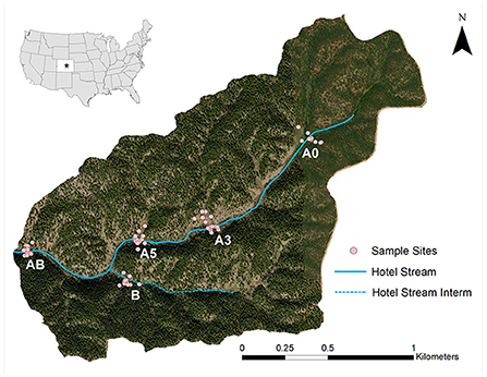
Figure 1. Sampling sites and stream reaches within the study area at Manitou Experimental Forest. Star on inset map indicates the location of the catchment.
Soil and stream sample collection and lab processing
At 62 sample locations within the catchment, bucket-type augers were used to sample from four depths: 10, 30, 50, and 100 centimeters (Table 1). Three replicate samples were taken at each sampling location, and each was sealed in a plastic bag to maintain field saturation. Location coordinates were recorded using a handheld GPS. Once collected, the samples were placed in coolers with ice packs for transportation to the laboratory and were stored in a −28°C freezer until processing.
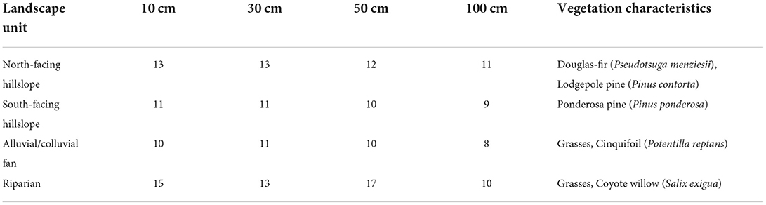
Table 1. Vegetation characteristics at each landscape unit and number of samples at each landscape unit and depth.
Soil samples were processed using a water extraction method to determine solute chemistry. Once thawed, large rocks and organic materials were removed from the soils using a 2 mm sieve. Next, 10 g of sieved soils were individually measured, placed in an Erlenmeyer flask, saturated with ultra-pure deionized water, overturned to mix the solution, and placed on a shaker table for 24 h at 200 rpm. Once removed from the shaker table, samples were placed in a centrifuge (ThermoFisher Sorvall ST 16) to separate the sediment from the extraction solution. Fifty mL of the soil solution was placed into centrifuge vial and spun at 5,000 rpm for 20 min. The supernatant water was then transferred from the centrifuge vials to HDPE bottles for filtering, removing most of the sediments. The extracted water samples were stored at 2°C and were filtered within 48 h of centrifuging.
Stream samples were collected daily to weekly from the end of the snowmelt in early May through early October 2020. Portable automatic samplers were installed at site AB during the summer months of 2020 to automatically collect daily stream samples (model-6712, Teledyne ISCO, Lincoln, NE, USA). Stream samples were collected in HDPE bottles and kept at 2°C until filtering within 24 h of collection. Stream stage data were recorded every 5 min at the most downstream site (AB), using a capacitance water level logger (Odyssey Dataflow Systems Limited) from May through early October 2020. Stage data were converted to discharge using a rating curve based on fifteen salt dilution measurements following Moore (2004).
All samples (soil supernatant and stream water) were filtered using vacuum-assisted filtering towers with glass microfiber filters (Whatman: 42 Nuclepore 1 μm glass microfiber filters, Grade GF/G). Filtered supernatant and stream samples were then transferred to opaque Nalgene bottles and frozen until solute concentration analysis. To measure solute concentrations, the filtered samples were analyzed by ion chromatography for both anions (F, Cl, NO2, Br, NO3, PO4, and SO4) and cations (Li, Na, NH4, K, Mg, and Ca). Sample duplicates along with analytical blanks and known standards were ran in each run to ensure instrument accuracy (±2.5% of the known concentrations from the standards).
Data analysis
To evaluate spatial and vertical differences among solutes, several series of t-tests were run among depths, landscape units, and depths at specific landscape units. Each solute distribution was found to be non-normal, thus, non-parametric t-tests (Wilcoxon Signed Rank test) were used for similarity testing. First, t-tests were run for each total solute at each landscape unit to identify any significant differences in solutes between depth for each landscape. Next, t-tests were run for average solute concentrations among all depths between landscape units to determine if there were any significant differences in concentration among different areas. Last, another series of t-tests were conducted among each landscape, for each solute, at every individual depth. These multiple statistical comparisons allowed us to identify differences in solute concentration among landscape units, depths, and landscape units at each depth. All t-tests were evaluated at the α = 0.05 level of significance.
To examine the relationship between spatial soil solutes and stream water chemistry, we used molar ratios to provide a normalized metric to compare stream and soil chemistry (Roy et al., 1999). We calculated the molar ratios K:Na, Ca:Mg, and NO3:Cl for both the soil extracts and the stream water samples by converting solute concentrations to molar concentrations and then dividing each of the chosen solutes by their respective atomic weights. The molar concentration of the solutes in the chosen ratios were divided (ex: K/Na) to calculate the molar ratio. A series of similarity tests were run between the stream and soil molar ratio data (Wilcoxon Signed Rank test). Comparisons were first made among all soil and stream molar ratios in bulk. Further comparisons were made among all soil molar ratios and stream molar ratios aggregated by season (fall, spring and summer) to see if hydrologic seasonality influenced the contribution of soil solutes in the stream. Then, molar ratio comparisons were made among soil sample landscape units and stream sample seasons. Molar ratios were then compared among the different sampling locations, subset by the stream along which they were sampled (A, B, or AB). Additionally, comparisons were made among bulk stream molar ratios and soil sample depth. Lastly, molar ratios for soil sample depths among each landscape unit was compared to bulk stream molar ratio data. All t-tests were evaluated at the α = 0.05 level of significance.
Results
Solute concentrations within each landscape unit
Concentrations of Br, and for the most part NO2, in the soil extracts were below the IC detection level; therefore, these solutes were not included in statistical comparisons. While significant differences were found among depths and landscapes in NO2, the differences in concentrations were minimal (0.21–0.35 mg/l; Table 3). Additionally, no significant differences were found in Na at any landscape unit across depths. No significant differences were found among any solutes (p < 0.05) between the north- and south-facing aspects of the riparian areas. Consequently, these data were combined when comparing the riparian area solutes to other landscape units.
Riparian differences with depth
Within the riparian landscape units, K and Ca differed across depths (Figure 2). For K, concentrations at 10 cm and >10 cm differed (p < 0.01), with mean concentrations ranging from 1.04 mg/l (100 cm) to 3.13 mg/l (10 cm), decreasing with depth (Table 2; Supplementary Figure 3). Mean Ca concentrations ranged from 2.67 mg/l (100 cm) to 4.21 mg/l (10 cm), decreasing with depth (Table 2). Calcium was found to have only borderline significance between 10 cm and 100 cm (p = 0.06) (Figure 2). Significant differences were found in F and SO4 for riparian landscapes across depths (Supplementary Figure 1). Fluoride concentrations differed between 10 cm and >10 cm (p < 0.05), and between 50 and 100 cm (p < 0.01) (Supplementary Figure 1). Mean concentrations of F ranged from 0.55 mg/l (10 cm) to 1.62 mg/l (100 cm), increasing with depth (Table 3). Sulfate showed a different pattern of significance across depths in riparian areas, with significant differences found between 10 and 30 cm, and 10 and 50 cm (p < 0.01) (Supplementary Figure 1). Concentrations of SO4 ranged from 0.69 mg/l (50 cm) and 1.00 mg/l (10 cm) with no clear pattern (increasing or decreasing) across depths (Table 3).
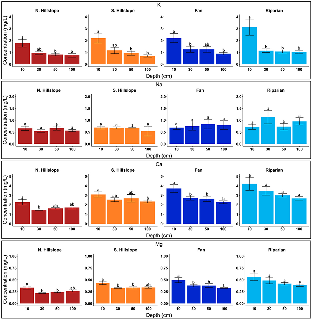
Figure 2. Bar charts displaying cation concentrations across sampled depths. Letters denote significance among depths at p < 0.05. Data presented are limited to solutes which were used for molar ratio comparisons with stream samples.
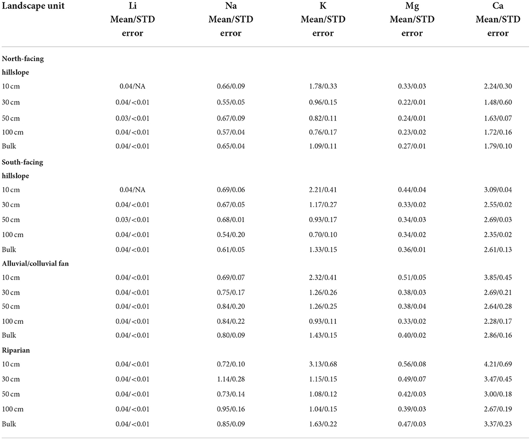
Table 2. Mean and standard error for each of the studied cation concentrations at each depth, and bulk, for every landscape unit.
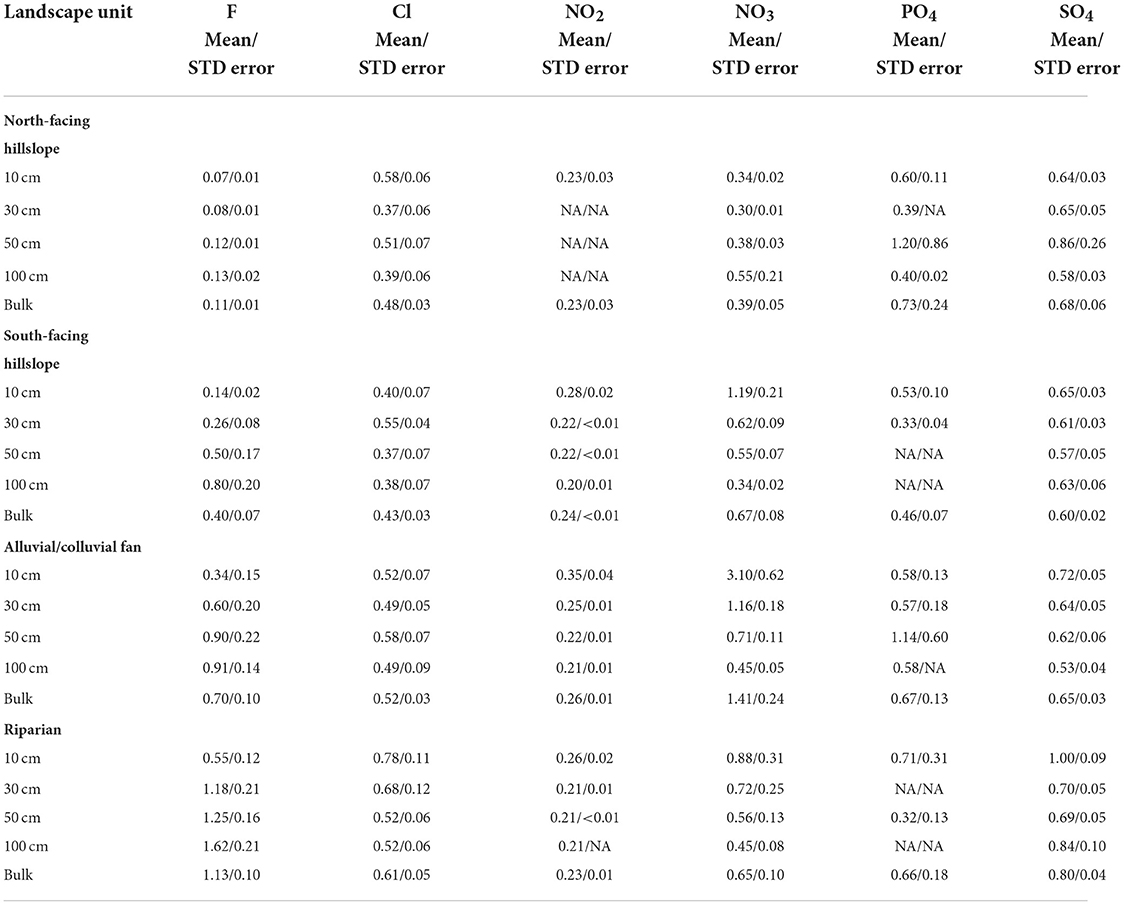
Table 3. Mean and standard error for each of the studied anion concentrations at each depth, and bulk, for every landscape unit.
Alluvial/colluvial fan differences with depth
We found significant differences in K, Mg, and Ca for alluvial/colluvial fans among the sampled depths (Figure 2; Supplementary Figure 3). Potassium showed significant differences between 10 and 100 cm, as well as borderline significance between 10 and 30 cm (p < 0.05) (Figure 2). Mean concentrations for K ranged from 0.93 mg/l (100 cm) to 2.32 mg/l (10 cm), decreasing with depth (Table 2). Significant differences in Mg were found between 10 and >10 cm (p < 0.01) (Figure 2). Mean concentrations of Mg ranged from 0.33 mg/l (100 cm) to 0.51 mg/l (10 cm), decreasing with depth (Table 2). Calcium had a similar pattern of significance as K, with significant differences found between 10 and >10 cm (p < 0.05) (Figure 2; Supplementary Figure 3). Mean concentrations of Ca ranged from 2.28 mg/l (100 cm) to 3.85 mg/l (10 cm), decreasing with depth slightly, but with a substantial drop in concentration below 10 cm (Table 2). Fluoride and NO3 also differed across depths (Figure 3; Supplementary Figures 1, 4). Fluoride had significant differences between 10 and >10 cm (p < 0.05) (Supplementary Figure 1), and mean concentration ranged from 0.34 mg/l (10 cm) to 0.91 mg/l (100 cm), increasing with depth (Table 3). Nitrate had significant differences between 10 and >10 cm (p < 0.01), with additional significant difference found between 30 and 100 cm (Figure 3; Supplementary Figure 4). Mean concentrations of NO3 were all relatively low and ranged from 0.45 mg/l (100 cm) to 0.88 (10 cm), decreasing with depth (Table 3).
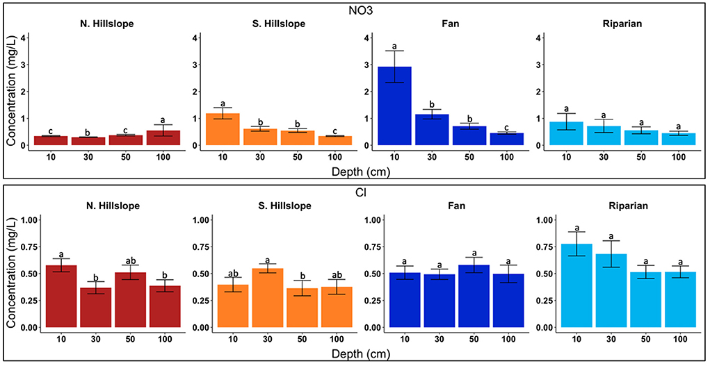
Figure 3. Bar charts displaying anion concentrations across sampled depths. Letters denote significance among depths at p < 0.05. Data presented are limited to solutes which were used for molar ratio comparisons with stream samples.
North-facing hillslope differences with depth
North-facing hillslopes had significant differences in Li, K, Mg, and Ca across depths (Figure 2; Supplementary Figure 3). While a significant difference was found between 50 and 100 cm (p < 0.01) for Li, concentrations only ranged 0.03 mg/l (50 cm) to 0.04 (10 cm) and were below the detection level for many samples, consequentially removing them from further analysis. Potassium had significant differences between 10 and 50 cm, as well as 10 and 100 cm (p < 0.05) (Figure 2; Supplementary Figure 3), with mean concentrations ranging from 0.76 mg/l (100 cm) to 1.78 mg/l (10 cm), decreasing with depth (Table 2). Significant differences in Mg concentrations were between 10 and 30 cm, as well as 10 and 50 cm (p < 0.01) (Figure 2; Supplementary Figure 3). Mean concentrations of Mg ranged from 0.22 mg/l (30 cm) to 0.33 mg/l (10 cm), with higher concentrations at 10 cm and relatively constant concentrations below 10 cm (Table 2). Calcium was found to have significant differences only between 10 and 30 cm (p < 0.05), with borderline significance between 10 and 100 cm (p = 0.055) (Figure 2). Mean concentrations ranged from 1.48 mg/l (30 cm) to 2.28 mg/l (10 cm), with a significantly higher concentration at 10 cm, and then increasing with depth slightly between 30–100 cm (Table 2).
Significant differences were found in F, Cl and NO3 concentrations in north-facing hillslopes at different depths (Figure 3; Supplementary Figures 1, 4). Fluoride concentrations differed between 10 and 50 cm (p < 0.01), as well as 10 and 100 cm (p < 0.05). We found differences among the intermediate depths as well with significant differences between 30 and 50 cm (p < 0.05), as well as 30 and 100 cm (p < 0.05) (Supplementary Figures 1, 4). Mean concentrations of F increased with depth, ranging from 0.074 mg/l (10 cm) to 0.13 mg/l (100 cm) (Table 3). Chloride was found to have significant differences at 10 and 30 cm (p < 0.05), as well as 10 and 100 cm (p < 0.05) (Figure 3). Concentration of Cl ranged from 0.37 mg/l (30 cm) to 0.58 mg/l (10 cm), with no obvious pattern across depths (Table 3). The only significant difference found for nitrate across depths was at 30 and 50 cm (p < 0.05) (Figure 3). Mean concentrations of NO3 ranged from 0.30 cm (30 cm) to 0.53 mg/l (100 cm), generally increasing with depth, but with the lowest concentration being at 30 cm (Table 3).
South-facing hillslope differences with depth
Within south-facing hillslopes, significant differences were found in K, Mg, and Ca (Figure 2). Potassium had significant differences between 10 and >10 cm (p < 0.05) (Figure 2; Supplementary Figure 3), with mean concentrations ranging from 0.70 mg/l (100 cm) to 2.21 mg/l (10 cm), decreasing with depth (Table 2). Significant differences in Mg were found between 10 and 30 cm, as well as 10 and 50 cm (p < 0.05) (Figure 2). Magnesium mean concentrations ranged from 0.33 mg/l (30 cm) to 0.44 mg/l (10 cm), with concentrations being generally consistent below 10 cm (Table 2). Significant differences in Ca were found between 10 cm and 100 cm (p < 0.05) (Figure 2). Concentrations of Ca ranged from 2.35 mg/l (100 cm) to 3.09 mg/l (10 cm), decreasing with depth (Table 2). Significant differences were found in F, NO3, and Cl in south-facing hillslopes at different depths (Supplementary Figures 1, 4; Figure 2). Fluoride was found to have significant differences between 10 and 50 cm (p < 0.05), and 10 cm and 100 cm (p < 0.05) (Supplementary Figure 1). Mean concentrations of F ranged from 0.14 mg/l (10 cm) to 0.80 mg/l (100 cm), increasing with depth (Table 3). Nitrate had one significant difference at depth between 30 and 50 cm (p < 0.05; Figure 3), and mean concentrations decreased with depth, ranging from 0.34 mg/l (100 cm) to 1.19 mg/l (10 cm) (Table 3). Chloride was found to be significantly different at depth only between 30 and 50 cm (p < 0.05) (Figure 3). Concentration of Cl ranged from 0.37 mg/l (50 cm) to 0.55 mg/l (30 cm), with generally higher concentrations in the shallower soils (Table 3).
Bulk differences among landscape units
Riparian areas vs. other landscape units
Significant differences in total cation concentrations from all depths between riparian and other landscape units were found for K, Mg, and Ca (Figure 4). Potassium concentrations differed between riparian and north-facing hillslope landscape units (p < 0.05) (Figure 4), with mean concentrations of 1.63 mg/l and 1.09 mg/l, respectively (Table 2). Magnesium differed between riparian and all other landscapes (p < 0.05) (Figure 4). Bulk Mg concentrations ranged from 0.27 mg/l to 0.47 mg/l with north-facing hillslopes being the lowest and riparian areas being the highest (Table 2). Calcium was found to have significant differences between riparian areas and the hillslopes (p < 0.01), as well as alluvial fans (p < 0.05) (Figure 4). Bulk Ca concentrations ranged from 3.37 mg/l at riparian areas to 1.79 mg/l at north-facing hillslopes (Table 2).
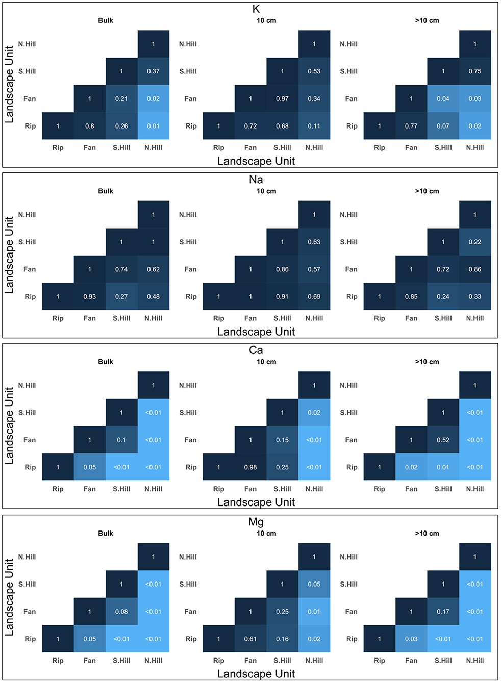
Figure 4. Significance matrices for non-parametric t-test comparisons of soil extract cations among different landscape units at each depth. The shade of the comparison is dependent on the level of significance, with lower p-values being lighter, and higher p-values being darker. Matrices shown are limited to solutes which were used for molar ratio comparisons with stream samples.
Significant differences in total anions concentration between riparian areas and other landscape units were found in F, Cl, NO3, and SO4 (Figure 5; Supplementary Figure 2). Fluoride was found to have significant differences between riparian areas and all other landscape units (p < 0.01) (Supplementary Figure 2). Mean concentrations of total F ranged from 0.11 mg/l to 1.13 mg/l, with north-facing hillslopes having the lowest concentration, and riparian having the greatest (Table 3). Chloride differed between riparian areas and south-facing hillslopes (p < 0.05) (Figure 5), with mean concentrations ranging from 0.43 mg/l in south-facing hillslopes to 0.61 mg/l in riparian areas (Table 3). Nitrate differed between riparian areas and north-facing hillslopes (p < 0.05), as well as riparian areas and alluvial/colluvial fans (p < 0.01) (Figure 5). Total mean concentrations of NO3 ranged from 0.39 to 1.41 mg/l, with the lowest concentrations being in north-facing hillslopes and the greatest in the alluvial/colluvial fans (Table 3). Total SO4 concentration were found to have significant differences among riparian areas and fans, as well as riparian areas and both aspects of hillslopes (p < 0.01) (Supplementary Figure 2). Mean concentrations of total SO4 ranged from 0.60 mg/l in south-facing hillslopes to 0.80 mg/l in riparian areas (Table 3).
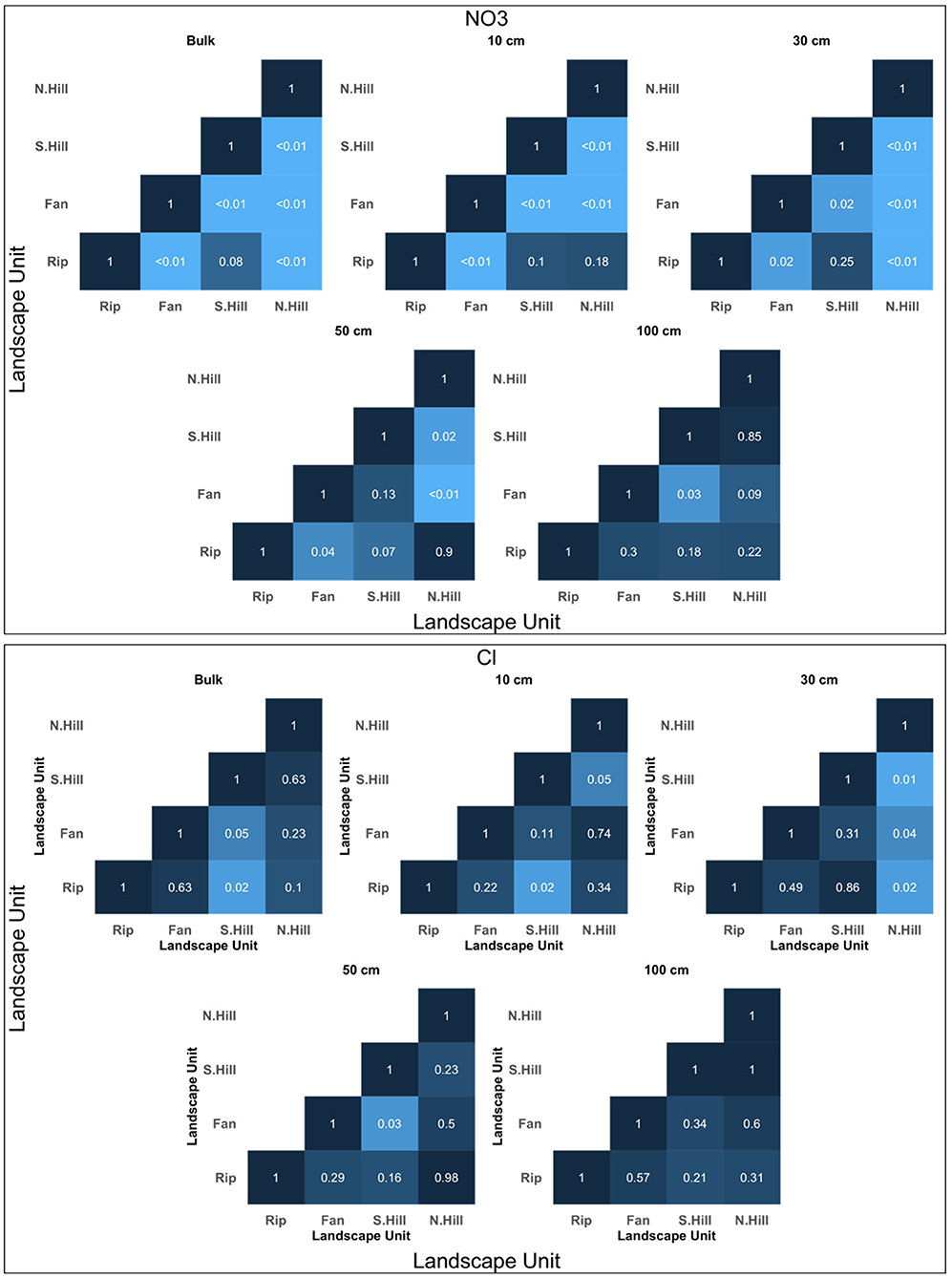
Figure 5. Significance matrices for t-test comparisons of anions among different landscape units at each depth. The shade of the comparison is dependent on the level of significance, with lower p-values being lighter, and higher p-values being darker. Matrices shown are limited to solutes which were used for molar ratio comparisons.
Alluvial/colluvial fans vs. other landscape units
In addition to the significant differences found between riparian and alluvial/colluvial fan landscapes, significant differences in total cations among alluvial/colluvial fans and other landscapes were found in K, Mg and Ca (Figure 4). Potassium concentrations differed between fans and north-facing hillslopes (p < 0.05). Magnesium was found to only have a significant difference between fans and north-facing hillslopes (p < 0.01) (Figure 4). Calcium concentrations differed between fans and north-facing hillslopes (Figure 4). Along with the significant differences found between riparian and alluvial/colluvial fan landscapes for anions, significant differences were also found between alluvial/colluvial fans and other landscape units for F, Cl, and NO3 (Figure 5; Supplementary Figure 2). Fluoride differed between fans and both aspects of the hillslopes (p < 0.05) (Supplementary Figure 2). Similarly, NO3 was also found to have significant differences between fans and both aspects of the hillslopes (p < 0.01) (Figure 5). Chloride concentrations differed between fans and south-facing hillslopes (p < 0.05) (Figure 5).
North- vs. south-facing hillslopes
In addition to the above noted comparisons, significant differences in cation concentrations were found between north- and south-facing hillslopes in Mg and Ca (p < 0.01) (Figure 4). Lastly, along with the significant comparisons evaluated above, significant differences in total cations were found between north- and south-facing hillslopes in F and NO3 (p < 0.01) (Figure 5, Supplementary Figure 2).
Comparisons between landscape units at depth
Based on the previous analyses, comparisons of solutes among each landscape unit at specific depths were limited to solutes which were found to have clear patterns in significant differences. Potassium, Mg, and Ca were evaluated at 10 and >10 cm depths. Differences in concentration for F and NO3 were evaluated for each sampled depth. Cl and SO4 were only analyzed at bulk concentrations, as they were found to only have significant differences among depths at a single landscape unit. The following analyses will build upon each other, with the previously noted landscape significance patterns being included in the analyses of the following landscape comparison.
Riparian vs. other landscape units
Differences at 10 cm: At 10 cm, riparian areas differed from all other landscape units in Mg, Ca, F, and NO3 concentrations. Magnesium differed between riparian areas and north-facing hillslopes (p < 0.05) (Figure 4). Similarly, Ca was found to have the same pattern of significance between riparian areas and north-facing hillslopes (p < 0.05) (Figure 4). Fluoride differed in concentrations among riparian areas and both aspects of the hillslopes (p < 0.01) (Supplementary Figure 2). Lastly, NO3 was found to only have significant differences between riparian areas and alluvial/colluvial fans (p < 0.01) (Figure 5).
Differences at >10 cm: For solutes analyzed at >10 cm, K, Mg, and Ca had significant differences between riparian and other landscape units. Potassium differed between riparian areas and north-facing hillslopes (p < 0.05) (Figure 4). Significant differences in Mg were found among riparian and all other landscape units (p < 0.05) (Figure 4). Calcium had a similar pattern to Mg, with significant differences among riparian areas and all other landscape units (p < 0.01) (Figure 4). Of the solutes evaluated at 30 cm, F and NO3 had significant differences among riparian areas and other landscape units. Fluoride concentrations differed among riparian areas and both aspects of the hillslopes (p < 0.01), with additional borderline significance found between riparian areas and fans (p = 0.055) (Supplementary Figure 2). Significant differences for NO3 at 30 cm were found between riparian areas and north-facing hillslopes (p < 0.01), as well as riparian areas and fans (p < 0.05) (Figure 5). Fluoride and NO3 both had significant differences between riparian areas and other landscape units at 50 cm. Similar to 30 cm, F was found to have significant differences in concentration among riparian areas and both aspects of hillslopes at 50 cm (p < 0.01) (Supplementary Figure 2). Nitrate differed between riparian and fan landscapes at 50 cm (p < 0.05) (Figure 5). At 100 cm, F was the only solute of those tested to have significant differences between riparian areas and other landscape units. Fluoride concentrations differed among riparian areas and all other landscape units (p < 0.05) (Supplementary Figure 2).
Alluvial/colluvial fan vs. other landscape units
Differences at 10 cm
In addition to the significance found between riparian areas and other landscape units, significant differences in solute concentrations between alluvial/colluvial fans and other landscape units were found in Mg, Ca, and NO3 and F. Magnesium was found to have significant differences between fans and north-facing hillslopes (p < 0.05) (Figure 4). Similarly, significant differences in Ca were only found between fans and north-facing hillslopes (p < 0.01) (Figure 4). Nitrate was found to have significant differences among fans and both aspects of hillslopes (p < 0.05) (Figure 5). Fluoride was found to have a significant difference between fans and north-facing hillslopes (p < 0.01) (Supplementary Figure 2).
Differences at >10 cm
For solutes evaluated at >10 cm, significant differences between fans and other landscape units were found in K, Mg, and Ca. Potassium concentrations were found to be significantly different between fans and both aspects of hillslopes (p < 0.05). For Mg, significant differences were found only between fans and north-facing hillslopes (p < 0.01) (Figure 4). Calcium was found to have a similar pattern, with a significant difference between fans and north-facing hillslopes (p < 0.01) (Figure 4). Of the solutes analyzed at 30 cm, significant differences in concentrations between fans and other landscape units were found in F NO3, and Cl. Fluoride was found to have significant differences between fans and north-facing hillslopes at 30 cm (p < 0.05) (Supplementary Figure 2). Nitrate was found to have significant differences in concentrations among fans and both aspects of the hillslopes (p < 0.05) (Figure 5). Chloride was found to have significant differences between fans and north-facing hillslopes at 30 cm (p < 0.05) (Figure 5). At 50 cm, significant differences in solute concentrations between fans and other landscape units were found in both F and NO3. For fluoride, significant differences were found between fans and north-facing hillslopes (p < 0.01) (Supplementary Figure 2). Nitrate was found to have a similar pattern, with differences between fans and north-facing hillslopes (p < 0.05) (Figure 5). At 100 cm, significant differences in solute concentration between fans and other landscape units were found in F and NO3. Significant differences in F were found between fans and north-facing hillslopes (p < 0.01) (Supplementary Figure 2). Nitrate differed fans and south-facing hillslopes in NO3 at 100 cm (p < 0.05) (Figure 5).
North- vs. south-facing hillslopes
As all other comparisons have been exhausted by the analysis detailed in the prior sections, only differences in solute concentrations between north- and south-facing hillslopes are addressed in this section. At 10 cm, significant differences between north-facing hillslopes and other landscape units (for the remaining comparisons) were found in Mg, Ca, F, and NO3 (p < 0.05 for all solutes; Figures 4, 5; Supplementary Figure 2). Of the solutes evaluated at >10 cm, significant differences among north-facing hillslopes and other landscape units at >10 cm were found in Mg and Ca. Both solutes were significant in north- and south-facing hillslope comparison (p < 0.01) (Figures 4, 5; Supplementary Figure 2). At 30 cm and 50 cm, NO3 and F concentrations differed among north-facing hillslopes and other landscape units (p < 0.05; Figure 5 and Supplementary Figure 2). At 100 cm, significant difference in solutes concentrations among north-facing hillslopes and other landscape units were found only for F (Supplementary Figure 2).
Comparisons among stream and soil solute molar ratios
Soil solute molar ratios were compared with stream solute molar ratios in bulk, among stream seasonality, soil sample landscape unit, soil and stream sampling location based on stream reach, soil sample depths, and soil sample landscape unit at depth. Average soil molar ratio amounts were 2.24 for K:Na, 4.28 for Ca:Mg, and 0.79 for NO3:Cl. Average stream molar ratio amounts were 0.22 for K:Na, 3.79 for Ca:Mg, and 0.22 for NO3:Cl. For all tested comparisons among the molar ratios of the soil extracts and the stream waters, we found significant differences (p < 0.05). In each comparison and for each of the considered molar ratios, mean values were higher in the soil samples than in the stream samples (Figure 6). It must be noted that the stream samples often yielded concentrations of NO3 below detection level, reducing the robustness of the NO3:Cl molar ratio and associated tests.
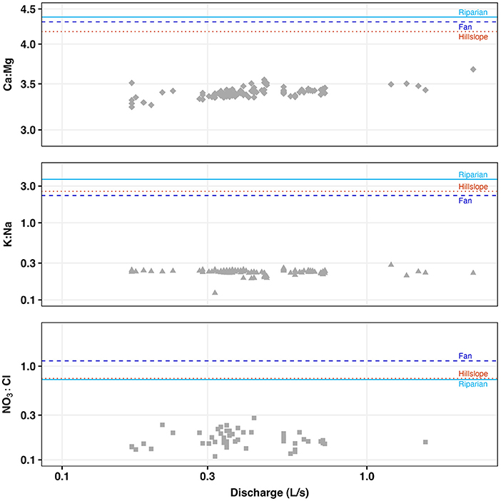
Figure 6. Molar ratio-discharge relationships of 2020 stream samples (gray) for Ca:Mg. K:Na, and NO3 in comparison to mean soil molar ratio values of the sampled landscape units (light blue, riparian; dark blue, alluvial/colluvial fans; orange, hillslopes).
Discussion
Solute concentrations between landscape units
Our findings indicate that aspect was not a control on solute concentrations in riparian and alluvial/colluvial fan landscapes; however, differences were found between north- and south-facing hillslopes. All solute concentrations were greater in the near-stream landscape units (riparian and alluvial/colluvial fan) than in the hillslopes, and nearly all solutes were higher in riparian areas than alluvial/colluvial fans (Tables 2, 3). Additionally, south-facing hillslopes were found to have higher concentrations than north-facing hillslopes in nearly all solutes (PO4 and SO4 were marginally higher on north-facing hillslopes). Increased concentrations of solutes in these near-stream landscape units was expected and can be partially due to the increased vegetation density leading to higher concentration of organically-derived solutes in riparian (willows, grasses, and forbs) and alluvial/colluvial fan areas (higher density of grassy vegetation), as well as the tendency for subsurface flow to flush downslope toward the stream (Christopher et al., 2006; Piatek et al., 2009; Jin et al., 2011; Herndon et al., 2018; Pei et al., 2021). Concentrations of organically-derived solutes, such as K and NO3 being greater in riparian and fan landscapes is clear, as there is expected to be more leaf litter and root materials (and their decomposition) in those soils when compared to hillslopes (Hedin et al., 1998; Piatek et al., 2009). Increased concentrations in near-stream units can also be spatially driven by the flushing of solutes from hillslopes toward riparian areas, which is consistent with the data found in this study (Jin et al., 2011; Covino, 2017; Mosimane et al., 2017). Additionally, areas with less dense, tree-dominated vegetation have generally been found to have greater rates of flushing and less solute retention of base anions and cations when compared to the dense grassy and willow dominated riparian areas (Pei et al., 2021).
Soil structure and texture influences solute retention and transport (Sullivan et al., 2022). Coarser soils with larger pore spaces more actively transport solutes through subsurface flow when compared to more dense and finer grained soils, explaining the increase in concentrations in riparian and fan landscapes as those soils were more dense and fine-grained than the hillslopes (Pei et al., 2021; NRCS, 2022). Additionally, soil with a relatively high clay fraction, as seen in the riparian and alluvial/colluvial fan areas, retain solutes more readily than coarser and sandier soils, further supporting the increase in most solute concentrations in riparian and alluvial/colluvial fan areas (Pei et al., 2021; NRCS, 2022). We did not complete a quantitative assessment of soil textures in this study, but a qualitative evaluation of the soils for riparian and alluvial/colluvial fans soils showed finer soils with higher clay content compared to those of the hillslopes.
While the vegetative and topographic explanations for solute behaviors are clear for differences between near-stream and hillslope landscapes, these factors do not clearly explain the increased concentrations of solutes in south-facing hillslopes when compared to north-facing hillslopes. The north-facing hillslopes, while having more vegetation and finer soils, were observed to have lower concentrations of solutes, working opposite of the processes described above (Tables 2, 3) (NRCS, 2022). A possible explanation is that preferential subsurface flowpaths along root systems could potentially flush the solutes from the north-facing hillslopes at a higher rate than on the south-facing hillslopes, because vegetation was denser in the north-facing aspect (Creed and Band, 1998; Pei et al., 2021). Additionally, higher soil moisture and cooler soil temperatures could contribute to lower solute concentrations in the north-facing hillslopes (Piatek et al., 2009). In addition to the flushing of solutes from hillslopes to valleys, wetter soils can dilute and transport soil solutes more readily when compared to drier soils, which have a higher level of solute retention (Piatek et al., 2009). The temperature of soils is also connected to wetness, as it had been found that warmer soils retain soil solutes more than cooler soils. Nitrate has been found to be flushed at particularly high rates in persistently wet soils and during snowmelt events (Creed and Band, 1998; McHale et al., 2002; Pei et al., 2021). Even with gradual topography, significant temperature differences between slope aspect occur due to the increased insolation that south-facing hillslopes receive compared to north-facing hillslopes (Rorison et al., 1986; Bennie et al., 2008). As the north-facing hillslopes are both cooler and wetter than the south-facing due to decreased direct insolation, greater canopy cover and delayed snowmelt, these processes could possibly explain the increased concentrations in south-facing hillslopes.
The amount of variation among landscape units differed among specific solutes, with some having larger differences in concentrations by location. Of the studied solutes, F, Ca, and NO3 had notably large variations among depths and landscape units (Tables 2, 3). Less spatial variation was found in SO4 and Cl, with higher concentrations in riparian areas than the other landscape units. For the geogenically-derived solutes (F, Ca, Cl, and SO4), these large differences between the riparian areas and hillslopes could be partially due to the deposition solutes from stream flow into the near-stream riparian areas. Geogenically-derived solutes in stream waters have been found to increase in summer months from an increased proportional contribution from groundwater, leading to the deposition of these solutes into the riparian areas, which could be a factor in the observed increase in solutes in riparian areas when compared to the hillslopes (McHale et al., 2002; Piatek et al., 2009). While variations of SO4 were less than other solutes, higher concentrations in riparian areas could be explained by the release of SO4 from the erosion and weathering of pyrite, a mineral prominent in MEF soils, which was then flushed down the hillslopes and remineralized in riparian areas from subsurface flow (Piatek et al., 2009; Herndon et al., 2018). Nitrate behaved differently than other solutes in that there were much higher concentrations in the fan landscapes than any other, and mean concentrations in riparian areas were closer to those of the hillslopes (Table 3). One possible explanation for this could be due to the particularly high transport of NO3 during snowmelt, rainfall events, and areas of high runoff (Creed et al., 1996; McHale et al., 2002; Piatek et al., 2009). While other solutes show a flushing pattern from the hillslopes to storage in the riparian areas, this behavior of NO3 to be flushed more actively in areas with high flow may be able to explain the high concentrations in fans, as there is not as much flow in the fans when compared to riparian landscapes (Creed et al., 1996; McHale et al., 2002; Piatek et al., 2009; van Meerveld et al., 2015).
Solute concentrations at depth
For nearly all of the studied solutes, mean concentrations either decreased with depth (K and NO3) or showed a clear pattern of high concentrations in shallow depth (10 cm) and constant lower concentrations below (30–50 cm) (Mg and Ca), with the exception of F, which increased with depth (Tables 2, 3). Smaller variations were found in Li, Na, Cl, and SO4, with more homogenous mean concentrations between depths. While this pattern of high surface concentrations was expected for the organically-derived solutes, it contrasted expectations for geogenically-sourced solutes like Mg and Ca, except for F. For the organic solutes, higher surface concentrations can be explained by greater amounts of leaf litter and roots within the shallowed depths (Christopher et al., 2006; Covino, 2017; Herndon et al., 2018). Calcium was particularly high in the surface level soils, which is supported by other studies finding high concentrations of Ca associated with the decomposition of plant material in shallow soils (Christopher et al., 2006). Reactive transport modeling efforts have shown that predicting near surface (< 200 cm) soil water concentrations of some geogenic species (e.g., Ca, Si, and K) can only be achieved by adding in vegetation nutrient cycling modules (Sullivan et al., 2019). Magnesium was expected to increase in concentration with depth due to its geogenic derivation, but did not follow this pattern and was found to have higher concentrations at shallower depths (Pei et al., 2021). This contrast in findings may be caused by the uptake and redeposition of Mg by plants within the catchment, making it behave more like the organically-derived solutes (Jin et al., 2011). Magnesium is a macronutrient for living plants and can be found in the leaf litter of pine species within MEF (Berg et al., 2021). While this process has been found to be minimal in other studies, this could be a driver for high surface concentrations of Mg within MEF, as the Pikes Peak granite bedrock of the area is poor in Mg (Smith, 1999; Jin et al., 2011). Another process that could lead to high concentrations of solutes in surface soils is evapoconcentration of solutes in shallow soils. While subsurface flow has a flushing effect on solutes, the evapoconcentration of solutes when the near surface soil is dried can lead to higher concentrations of solutes above the deeper subsurface (Mosimane et al., 2017). High surface levels of K, Mg, Ca, Cl, and SO4 have been attributed to evapoconcentration in previous studies and is supported by the data of this study as well (Mills, 2016; Mosimane et al., 2017).
Of the studied geogenically-derived solutes, F was the only one to show the expected pattern of increasing concentrations with depth. This was the case across all landscape units; however, there was more variation within the fans and south-facing hillslopes than riparian areas and north-facing hillslopes (Table 3). This clear pattern of increase in depth may be attributed to the high concentration of F within the Pikes Peak granite bedrock being weathered through subsurface flow (Smith, 1999). The decreased variability with depth in the riparian areas and north-facing hillslopes may be caused by the trend of increased flushing on the north-facing hillslopes, and the consequent channeling of concentrations within the downslope riparian areas across all depths (Piatek et al., 2009).
Simple model of runoff generation and comparison to other studies
Our results from comparing molar ratios between the stream and soils suggest that shallow, lateral subsurface or soil matrix flow is not a large contributor to streamflow in this system. While previous studies have found that shallow soils can be chemically connected to streams, particularly in storm conditions and agricultural environments, our findings indicate little chemical connectivity between the streams and shallow soils (Figure 6; McGuire and McDonnell, 2010; Jencso and McGlynn, 2011; Zhi and Li, 2020). While chemo-dynamic soil solute patterns have been observed with changing seasons in other studies, additional temporal sampling would needed to evaluate this within MEF (Xiao et al., 2021). We speculate that the lack of connection between the soil and the stream is indicative of a system that is dominated by deeper groundwater flowpaths. Stream water and soil sampling during storm events, as well as groundwater sampling, would allow for a more insightful analysis of subsurface contribution to stream chemistry in this catchment; however, this intensity of sampling was beyond the scope of this study.
Our observed spatial patterns of soil solute concentrations both confirm and contrast findings of previous studies regarding soil solute transport and spatial variations. Generally, this system displayed expected patterns of solute concentrations among depths and landscape units throughout the catchment. Biogenically-sourced solutes were found to be in higher concentration near the surface when compared to deeper samples, and in landscape units with more dense vegetation. However, many geogenic solutes, in particular Mg, contrasted our expectations with concentrations higher in near-surface soils which is most-likely caused by bioaccumulation in leaf litter (Berg et al., 2021; Xiao et al., 2021). This pattern among geogenic solutes appears to be site specific, with expected patterns being displayed in F, which is prominent in the catchment's bedrock material (Smith, 1999). Topographically, solute concentrations were found to follow the trends of previous studies in unaltered catchments, displaying a slight flushing pattern in shallow soils, indicated by the accumulation of solutes in the near-stream landscape units (Jin et al., 2011; Covino, 2017; Mosimane et al., 2017; Zhi and Li, 2020; Xiao et al., 2021).
Possible hydrologic tracers
When evaluating the data for possible hydrologic flow tracers, factors include which solutes were found to have distinct patterns among landscape units and at depths. When patterns of variation can be identified between these two factors, where subsurface flow occurs both spatially and vertically can be inferred (Reza et al., 2017). Our initial results of variation in solutes across landscape units and depth suggested that K, Ca, NO3, and F could possibly be valuable solute tracers within Hotel Gulch as each had distinct patterns of variation either spatially, at depth, or both. While the lack of stream and soil connectivity found in this study restricts the amount of inference that can be made about stream solute source locations and subsurface flow dynamics, these solutes could be of interest in future studies evaluating solute chemistry in the catchment, as they display significant variability.
Lastly, our use of ultra-pure deionized water rather than simulated rainwater solutions could influence the measured concentrations of solutes extracted from the soil. Use of pure water as the eluent in this soil extraction experiment targets water-soluble constituents in soil that are expected to be the weakest bound forms in the solid phase (Takeda et al., 2006). Alternative extraction solutions such as using dilute unbuffered salts formulated to simulate precipitation would be expected to be slightly more aggressive and also release exchangeable ions in the soil (Jones and Willett, 2006). Solute concentrations of rain at the MEF are dilute and ranged from < 0.3 mg/l (e.g., Li and NH4) to 1.7 mg/l (Ca) and therefore, we would not expect the rain to substantially increase the exchange or release of solutes in comparison to the deionized water used in this study.
Conclusion
Through the sampling and analysis of ~200 samples within a headwater catchment of MEF, we examined the spatial variation in soil solutes and how the solutes may be used as tracers of hydrologic flowpaths to the stream. Of the studied soil solutes, it was found that K, Ca, F, and NO3 could potentially be valuable tracers of subsurface flow through a catchment and provide information on how and where water is traveling beneath the surface toward a stream. Several solutes such as K, NO3, and Mg, were found to be in high concentration in near surface soils (10 cm) and in densely vegetated areas, displaying an importance of biotic cycling for solute accumulation and transport within the catchment. However, using molar ratios to compare soil extracts to stream water indicated that shallow subsurface flow through the soil was not likely to be a major contributor to stream water chemistry. This study provides a local and physical evaluation of topographic effects on soil water chemistry, both confirming the found unchanged behaviors of many solute relationships under differing discharge levels, while also contrasting expectations in certain solutes patterns such as Mg. While limitations to the depth of which inferences can be made based on this study exist, it can be used as a preliminary resource for further study of soil solute behaviors, tracers within a catchment, and their implications on water quality and availability.
Data availability statement
The datasets presented in this study can be found in online repositories. The names of the repository/repositories and accession number(s) can be found at: https://www.hydroshare.org/resource/7a3958db102649998d7e0dd5b008c023/.
Author contributions
RG: conceptualization, formal analysis, investigation, data curation, visualization, and writing–original draft. SB: conceptualization, software, data curation, and writing–review and editing. HB: conceptualization, methodology, resources, validation, writing–reviewing and editing, supervision, and funding acquisition. PS: conceptualization, validation, and writing–reviewing and editing. All authors contributed to the article and approved the submitted version.
Funding
This study was supported by the National Science Foundation: Award Numbers 2021669 and 2012796.
Acknowledgments
Ethan Burns, Sáde Cromratie Clemons, Mykael Pineda, Hallie Adams, Katarena Matos, Kyotaek Hwang, and Matthew Schiff provided field and laboratory assistance. Thank-you to Eve-Lyn Hinckley, Wendy Freeman Roth, and Kathy Welch for technical assistance. Special thanks to the US Forest Service Rocky Mountain Research Station for facilitating research at the Manitou Experimental Forest and the University of Colorado-Boulder Honors Program and Department of Geography for encouraging undergraduate research opportunities.
Conflict of interest
The authors declare that the research was conducted in the absence of any commercial or financial relationships that could be construed as a potential conflict of interest.
Publisher's note
All claims expressed in this article are solely those of the authors and do not necessarily represent those of their affiliated organizations, or those of the publisher, the editors and the reviewers. Any product that may be evaluated in this article, or claim that may be made by its manufacturer, is not guaranteed or endorsed by the publisher.
Author disclaimer
Any opinions, findings, and conclusions or recommendations expressed in this article are those of the author(s) and do not necessarily reflect the views of the National Science Foundation.
Supplementary material
The Supplementary Material for this article can be found online at: https://www.frontiersin.org/articles/10.3389/frwa.2022.1003968/full#supplementary-material
References
Andrews, D. M., Lin, H., Zhu, Q., Jin, L., and Brantley, S. L. (2011). Hot spots and hot moments of dissolved organic carbon export and soil organic carbon storage in the shale hills catchment. Vadose Zone J. 10, 943–954. doi: 10.2136/vzj2010.0149
Bennie, J., Huntley, B., Wiltshire, A., Hill, M., and Baxter, R. (2008). Slope, aspect and climate: Spatially explicit and implicit models of topographic microclimate in chalk grassland. Ecol. Model. 216, 47–59. doi: 10.1016/j.ecolmodel.2008.04.010
Berg, B., and Laskowski, R. (1997). Changes in nutrient concentrations and nutrient release in decomposing needle litter in monocultural systems of Pinus contorta and Pinus sylvestris—a comparison and synthesis. Scand. J. For. Res. 12, 113–121. doi: 10.1080/02827589709355392
Berg, B., Sun, T., Johansson, M.-B., Sanborn, P., Ni, X., Åkerblom, S., et al. (2021). Magnesium dynamics in decomposing foliar litter – A synthesis. Geoderma 382, 114756. doi: 10.1016/j.geoderma.2020.114756
Bhat, S. U., Khanday, S. A., Islam, S. T., and Sabha, I. (2021). Understanding the spatiotemporal pollution dynamics of highly fragile montane watersheds of Kashmir Himalaya, India. Environ. Pollut. 286, 117335. doi: 10.1016/j.envpol.2021.117335
Botter, M., Li, L., Hartmann, J., Burlando, P., and Fatichi, S. (2020). Depth of solute generation is a dominant control on concentration-discharge relations. Water Resour. Res. 56, 695. doi: 10.1029/2019WR026695
Bukoski, I. S., Murphy, S. F., Birch, A. L., and Barnard, H. R. (2021). Summer runoff generation in foothill catchments of the Colorado Front Range. J. Hydrol. 595, 125672. doi: 10.1016/j.jhydrol.2020.125672
Bushnell, T. M. (1943). Some aspects of the soil catena concept. Soil Sci. Soc. Am. J. 7, 466–476. doi: 10.2136/sssaj1943.036159950007000C0079x
Chorover, J., Derry, L. A., and McDowell, W. H. (2017). Concentration-Discharge Relations in the Critical Zone: Implications for Resolving Critical Zone Structure, Function, and Evolution. Water Resour. Res. 53, 8654–8659. doi: 10.1002/2017WR021111
Christopher, S. F., Page, B. D., Campbell, J. L., and Mitchell, M. J. (2006). Contrasting stream water NO3– and Ca2+ in two nearly adjacent catchments: the role of soil Ca and forest vegetation. Glob. Change Biol. 12, 364–381. doi: 10.1111/j.1365-2486.2005.01084.x
Covino, T. (2017). Hydrologic connectivity as a framework for understanding biogeochemical flux through watersheds and along fluvial networks. Geomorphology 277, 133–144. doi: 10.1016/j.geomorph.2016.09.030
Creed, I. F., and Band, L. E. (1998). Export of nitrogen from catchments within a temperate forest: Evidence for a unifying mechanism regulated by variable source area dynamics. Water Resour. Res. 34, 3105–3120. doi: 10.1029/98WR01924
Creed, I. F., Band, L. E., Foster, N. W., Morrison, I. K., Nicolson, J. A., Semkin, R. S., et al. (1996). Regulation of nitrate-n release from temperate forests: a test of the n flushing hypothesis. Water Resour. Res. 32, 3337–3354. doi: 10.1029/96WR02399
Dai, W., Li, Y., Fu, W., Jiang, P., Zhao, P., Li, Y., et al. (2018). Spatial variability of soil nutrients in forest areas: A case study from subtropical China. J. Plant Nutr. Soil Sci. 181, 827–835. doi: 10.1002/jpln.201800134
Frank, J. M., Fornwalt, P. F., Asherin, L. A., and Alton, S. K. (2021). Manitou Experimental Forest Hourly Meteorology Data. 3rd Edition. Fort Collins CO: Forest Service Research Data Archive.
Godsey, S. E., Hartmann, J., and Kirchner, J. W. (2019). Catchment chemostasis revisited: Water quality responds differently to variations in weather and climate. Hydrol. Process. 33, 3056–3069. doi: 10.1002/hyp.13554
Godsey, S. E., Kirchner, J. W., and Clow, D. W. (2009). Concentration–discharge relationships reflect chemostatic characteristics of US catchments. Hydrol. Process. 23, 1844–1864. doi: 10.1002/hyp.7315
Gomi, T., Sidle, R. C., and Richardson, J. S. (2002). Understanding Processes and Downstream Linkages of Headwater Systems: Headwaters differ from downstream reaches by their close coupling to hillslope processes, more temporal and spatial variation, and their need for different means of protection from land use. BioScience 52, 905–916. doi: 10.1641/0006-3568(2002)0520905:UPADLO2.0.CO;2
Hale, K. E., Wlostowski, A. N., Badger, A. M., Musselman, K. N., Livneh, B., and Molotch, N. P. (2022). Modeling streamflow sensitivity to climate warming and surface water inputs in a montane catchment. J. Hydrol. Reg. Stud. 39, 100976. doi: 10.1016/j.ejrh.2021.100976
Hedin, L. O., von Fischer, J. C., Ostrom, N. E., Kennedy, B. P., Brown, M. G., and Robertson, G. P. (1998). Thermodynamic constraints on nitrogentransformations and other biogeochemicalprocesses at soil–stream interfaces. Ecology 79, 684–703. doi: 10.1890/0012-9658(1998)0790684:TCONAO2.0.CO;2
Herndon, E. M., Dere, A. L., Sullivan, P. L., Norris, D., Reynolds, B., and Brantley, S. L. (2015). Landscape heterogeneity drives contrasting concentration–discharge relationships in shale headwater catchments. Hydrol. Earth Syst. Sci. 19, 3333–3347. doi: 10.5194/hess-19-3333-2015
Herndon, E. M., Steinhoefel, G., Dere, A. L. D., and Sullivan, P. L. (2018). Perennial flow through convergent hillslopes explains chemodynamic solute behavior in a shale headwater catchment. Chem. Geol. 493, 413–425. doi: 10.1016/j.chemgeo.2018.06.019
Hook, P. B., and Burke, I. C. (2000). Biogeochemistry in a shortgrass landscape: control by topography, soil texture, and microclimate. Ecology 81, 2686–2703. doi: 10.1890/0012-9658(2000)0812686:BIASLC2.0.CO;2
Jencso, K. G., and McGlynn, B. L. (2011). Hierarchical controls on runoff generation: Topographically driven hydrologic connectivity, geology, and vegetation. Water Resour. Res. 47, 10666. doi: 10.1029/2011WR010666
Jin, L., Andrews, D. M., Holmes, G. H., Lin, H., and Brantley, S. L. (2011). Opening the “Black Box”: water chemistry reveals hydrological controls on weathering in the susquehanna shale hills. Vadose Zone J. 10, 928–942. doi: 10.2136/vzj2010.0133
Jin, L., Ogrinc, N., Yesavage, T., Hasenmueller, E. A., Ma, L., Sullivan, P. L., et al. (2014). The CO2 consumption potential during gray shale weathering: Insights from the evolution of carbon isotopes in the Susquehanna Shale Hills critical zone observatory. Geochim. Cosmochim. Acta 142, 260–280. doi: 10.1016/j.gca.2014.07.006
Jones, D. L., and Willett, V. B. (2006). Experimental evaluation of methods to quantify dissolved organic nitrogen (DON) and dissolved organic carbon (DOC) in soil. Soil Biol. Biochem. 38, 991–999. doi: 10.1016/j.soilbio.2005.08.012
Kaiser, K. E., and McGlynn, B. L. (2018). Nested scales of spatial and temporal variability of soil water content across a semiarid montane catchment. Water Resour. Res. 54, 7960–7980. doi: 10.1029/2018WR022591
Kiewiet, L., van Meerveld, I., Stähli, M., and Seibert, J. (2020). Do stream water solute concentrations reflect when connectivity occurs in a small, pre-Alpine headwater catchment? Hydrol. Earth Syst. Sci. 24, 3381–3398. doi: 10.5194/hess-24-3381-2020
Langhammer, J., and Bernsteinová, J. (2020). Which aspects of hydrological regime in mid-latitude montane basins are affected by climate change? Water 12, 2279. doi: 10.3390/w12082279
Li, L., Sullivan, P. L., Benettin, P., Cirpka, O. A., Bishop, K., Brantley, S. L., et al. (2021). Toward catchment hydro-biogeochemical theories. WIREs Water 8, e1495. doi: 10.1002/wat2.1495
McGuire, K. J., and McDonnell, J. J. (2010). Hydrological connectivity of hillslopes and streams: Characteristic time scales and nonlinearities. Water Resour. Res. 46, W10543. doi: 10.1029/2010WR009341
McHale, M. R., McDonnell, J. J., Mitchell, M. J., and Cirmo, C. P. (2002). A field-based study of soil water and groundwater nitrate release in an Adirondack forested watershed. Water Resour. Res. 38, 16. doi: 10.1029/2000WR000102
Mills, T. J. (2016). Water Chemistry Under a Changing Hydrologic Regime: Investigations into the Interplay Between Hydrology and Water-Quality in Arid and Semi-Arid Watersheds in Colorado, USA (Ph.D.). Colorado, USA: University of Colorado at Boulder.
Milne, G. (1936). Normal erosion as a factor in soil profile development. Nature 138, 548–549. doi: 10.1038/138548c0
Milne, G. (1947). A Soil Reconnaissance Journey Through Parts of Tanganyika Territory December 1935 to February 1936. J. Ecol. 35, 192–265. doi: 10.2307/2256508
Molina, A., Vanacker, V., Corre, M. D., and Veldkamp, E. (2019). Patterns in soil chemical weathering related to topographic gradients and vegetation structure in a high andean tropical ecosystem. J. Geophys. Res. Earth Surf. 124, 666–685. doi: 10.1029/2018JF004856
Moore, R. D. (2004). Introduction to salt dilution gauging for streamflow measurement part 2: constant-rate injection. Streamline, Watershed Manage. Bull. 8, 11–15.
Mosimane, K., Struyf, E., Gondwe, M. J., Frings, P., vanPelt, D., Wolski, P., et al. (2017). Variability in chemistry of surface and soil waters of an evapotranspiration-dominated flood-pulsed wetland: solute processing in the Okavango Delta, Botswana. Water SA. 43, 104–115. doi: 10.4314/wsa.v43i1.13
Newman, B. D., Campbell, A. R., and Wilcox, B. P. (1998). Lateral subsurface flow pathways in a semiarid Ponderosa pine hillslope. Water Resour. Res. 34, 3485–3496. doi: 10.1029/98WR02684
NRCS (2022). Custom Soil Resource Report for Pike National Forest, Eastern Part, Colorado, Parts of Douglas, El Paso, Jefferson, and Teller Counties.
Opedal, Ø. H., Armbruster, W. S., and Graae, B. J. (2015). Linking small-scale topography with microclimate, plant species diversity and intra-specific trait variation in an alpine landscape. Plant Ecol. Divers. 8, 305–315. doi: 10.1080/17550874.2014.987330
Ortega, J., Turnipseed, A., Guenther, A. B., Karl, T. G., Day, D. A., Gochis, D., et al. (2014). Overview of the Manitou Experimental Forest Observatory: site description and selected science results from 2008 to (2013). Atmospheric Chem. Phys. 14, 6345–6367. doi: 10.5194/acp-14-6345-2014
Pei, Y., Huang, L., Li, D., and Shao, M. (2021). Characteristics and controls of solute transport under different conditions of soil texture and vegetation type in the water–wind erosion crisscross region of China's Loess Plateau. Chemosphere 273, 129651. doi: 10.1016/j.chemosphere.2021.129651
Piatek, K. B., Christopher, S. F., and Mitchell, M. J. (2009). Spatial and temporal dynamics of stream chemistry in a forested watershed. Hydrol. Earth Syst. Sci. 13, 423–439. doi: 10.5194/hess-13-423-2009
Reza, S. K., Nayak, D. C., Mukhopadhyay, S., Chattopadhyay, T., and Singh, S. K. (2017). Characterizing spatial variability of soil properties in alluvial soils of India using geostatistics and geographical information system. Arch. Agron. Soil Sci. 63, 1489–1498. doi: 10.1080/03650340.2017.1296134
Rorison, I. H., Sutton, F., and Hunt, R. (1986). Local climate, topography and plant growth in Lathkill Dale NNR. I. A twelve-year summary of solar radiation and temperature. Plant Cell Environ. 9, 49–56. doi: 10.1111/j.1365-3040.1986.tb01722.x
Roy, S., Gaillardet, J., and Allègre, C. J. (1999). Geochemistry of dissolved and suspended loads of the Seine River, France: anthropogenic impact, carbonate and silicate weathering. Geochim. Cosmochim. Acta 63, 1277–1292. doi: 10.1016/S0016-7037(99)00099-X
Sadiq, F. K., Maniyunda, L. M., Anumah, A. O., and Adegoke, K. A. (2021). Variation of soil properties under different landscape positions and land use in Hunkuyi, Northern Guinea savanna of Nigeria. Environ. Monit. Assess. 193, 178. doi: 10.1007/s10661-021-08974-7
Seibert, J., Stendahl, J., and Sørensen, R. (2007). Topographical influences on soil properties in boreal forests. Geoderma 141, 139–148. doi: 10.1016/j.geoderma.2007.05.013
Seidl, R., Thom, D., Kautz, M., Martin-Benito, D., Peltoniemi, M., Vacchiano, G., et al. (2017). Forest disturbances under climate change. Nat. Clim. Change 7, 395–402. doi: 10.1038/nclimate3303
Smith, D. R. (1999). A review of the Pikes Peak batholith, Front Range, central Colorado: A “type example” of A-type granitic magmatism. Rocky Mt. Geol. 34, 289–312. doi: 10.2113/34.2.289
Sullivan, P. L., Billings, S. A., Hirmas, D., Li, L., Zhang, X., Ziegler, S., et al. (2022). Embracing the dynamic nature of soil structure: A paradigm illuminating the role of life in critical zones of the Anthropocene. Earth-Sci. Rev. 225, 103873. doi: 10.1016/j.earscirev.2021.103873
Sullivan, P. L., Goddéris, Y., Shi, Y., Gu, X., Schott, J., Hasenmueller, E. A., et al. (2019). Exploring the effect of aspect to inform future earthcasts of climate-driven changes in weathering of shale. J. Geophys. Res. Earth Surf. 124, 974–993. doi: 10.1029/2017JF004556
Takeda, A., Tsukada, H., Takaku, Y., Hisamatsu, S., Inaba, J., and Nanzyo, M. (2006). Extractability of major and trace elements from agricultural soils using chemical extraction methods: Application for phytoavailability assessment. Soil Sci. Plant Nutr. 52, 406–417. doi: 10.1111/j.1747-0765.2006.00066.x
USFS, (2019). Manitou Experimental Forest [WWW Document]. Rocky Mountain Research Station. Available online at: https://www.fs.usda.gov/rmrs/experimental-forests-and-ranges/manitou-experimental-forest (accessed March 1, 2022).
van Meerveld, H. J., Seibert, J., and Peters, N. E. (2015). Hillslope–riparian-stream connectivity and flow directions at the Panola Mountain Research Watershed. Hydrol. Process. 29, 3556–3574. doi: 10.1002/hyp.10508
Wen, H., Perdrial, J., Abbott, B. W., Bernal, S., Dupas, R., Godsey, S. E., et al. (2020). Temperature controls production but hydrology regulates export of dissolved organic carbon at the catchment scale. Hydrol. Earth Syst. Sci. 24, 945–966. doi: 10.5194/hess-24-945-2020
Xiao, D., Brantley, S. L., and Li, L. (2021). Vertical connectivity regulates water transit time and chemical weathering at the hillslope scale. Water Resour. Res. 57, e2020WR029207. doi: 10.1029/2020WR029207
Zhi, W., and Li, L. (2020). The shallow and deep hypothesis: subsurface vertical chemical contrasts shape nitrate export patterns from different land uses. Environ. Sci. Technol. 54, 11915–11928. doi: 10.1021/acs.est.0c01340
Keywords: soil solutes, montane forest, flowpath, hydrologic tracers, molar ratio, critical zone, undergraduate research
Citation: Gregory RB, Bush SA, Sullivan PL and Barnard HR (2022) Examining spatial variation in soil solutes and flowpaths in a semi-arid, montane catchment. Front. Water 4:1003968. doi: 10.3389/frwa.2022.1003968
Received: 26 July 2022; Accepted: 12 October 2022;
Published: 09 November 2022.
Edited by:
Alexandra Ponette-Gonzalez, University of North Texas, United StatesReviewed by:
Michelle E. Newcomer, Berkeley Lab (DOE), United StatesNathan Conroy, Los Alamos National Laboratory (DOE), United States
Copyright © 2022 Gregory, Bush, Sullivan and Barnard. This is an open-access article distributed under the terms of the Creative Commons Attribution License (CC BY). The use, distribution or reproduction in other forums is permitted, provided the original author(s) and the copyright owner(s) are credited and that the original publication in this journal is cited, in accordance with accepted academic practice. No use, distribution or reproduction is permitted which does not comply with these terms.
*Correspondence: Holly R. Barnard, aG9sbHkuYmFybmFyZEBjb2xvcmFkby5lZHU=