A Hybrid Dataset of Historical Cool-Season Lake Effects From the Eastern Great Lakes of North America

The moistening of cold air passing over the Great Lakes of North America has a profound impact on the cool season climate of regions downwind, from relatively benign air mass modification to highly-impactful snowfall events. The importance of lake effects has led to the development of varying techniques for systematically identifying lake-effect days. The results of two such methods are merged here to yield a more thorough record of lake-effect days for the eastern Great Lakes. Comparative analysis of the data sets illustrates the different objectives of the two methodologies, where one identifies days with a synoptic setup conducive to lake-effect snowfall, and the other identifies days with lake-effect modification of the overlying air mass. A smaller population of “absolute” lake-effect days are those identified by both methods, while a larger population of “hybrid” lake-effect days are absolute days plus those identified by one method but not the other. For a 51-year study period ending with the 2014–15 cool season, the absolute data set yields a mean of about 15 lake-effect days per year, or 8% of the November through April season, while the hybrid data set yields a mean of 56 lake-effect days per year, or 31% of the season. The frequencies of absolute, air mass modification-defined, and hybrid lake-effect days decreased through the study period, with days within the hybrid data set declining at a statistically significant rate of 2.8 days per decade, although most obviously from the late 1970s through the early 2000s. The result is a general drying of the cool-season lake-effect hydroclimate. The merged data set offers a more thorough historical record of days available for atmospheric and hydroclimatic study of the lake-effect phenomenon within the eastern Great Lakes region.

Introduction

Like a number of water bodies globally, the Great Lakes of North America (Figure 1) are capable of modifying the thermal and moisture characteristics of the lower atmosphere, altering the weather and climate of areas downwind (Andresen, 2012; Notaro et al., 2013). Great Lakes “lake effects” are most distinct early within the cool season, when energy that has accumulated within the lakes during the warmth of the year interacts with southward moving cold air. The vertical stability of the deeply cold atmosphere is reduced with low-level warming and moistening, initiating upward motion that is often enhanced by friction above the land surface downwind to yield clouds and lake-effect precipitation (Scott and Huff, 1996). The result is an acute impact on the weather and hydroclimate of areas generally east and southeast of each lake. The advection of cold air across the lakes is typically associated with a rather distinct weather pattern, most often involving some variation of a surface low-pressure center to the east and surface high-pressure to the west (Ellis and Leathers, 1996; Suriano and Leathers, 2017a). The integrated portrayal of atmospheric pressure centers and the air masses arranged around them is referenced as the synoptic atmosphere; thus, the cool season effect of the Great Lakes, with distinct cold air advection between opposing pressure centers, is a phenomenon that lends itself to synoptic atmospheric classification techniques.

FIGURE 1

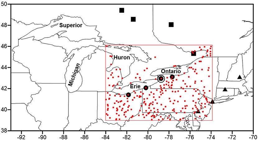
Figure 1. The North American Great Lakes and the locations of GHCN-Daily precipitation stations (red squares within red boundary), the location of Buffalo, New York (large open circle) for which Suriano and Leathers (2017a) constructed a Temporal Synoptic Index, and the three sets of four locations for which Spatial Synoptic Classification data were applied by Ellis et al. (2021), with black-filled circles representing lake-effect stations, and black-filled squares and triangles representing northern and eastern non-lake-effect stations.

The Temporal Synoptic Index (TSI) has been used effectively to identify cool season synoptic atmospheric patterns conducive to lake-effect precipitation within the historical record (Ellis and Leathers, 1996; Suriano and Leathers, 2017a). The TSI method (Kalkstein and Corrigan, 1986) involves using principal components analysis (PCA) on 24 daily weather observations (six variables, four times per day) to determine primary modes of variability seasonally. Average linkage clustering is then used to cluster PCA component scores with large eigenvalues to yield clusters of days, or synoptic types, with a similar surface meteorological profile. Most recently, Suriano and Leathers (2017a) applied the TSI methodology to daily data for Buffalo, New York (Figure 1) to identify synoptic patterns conducive to lake-effect snowfall downwind of the eastern Great Lakes Erie and Ontario. The TSI was constructed using data for the autumn (September–November), winter (December–February), and spring (March–May) seasons separately. Suriano and Leathers (2017a) identified seven TSI types conducive to lake-effect snowfall based on composites of their sea-level pressure pattern, lower-atmospheric wind direction and speed, vertical wind direction shear through the lower atmosphere, and temperature difference between the lake surface and lower atmosphere. The latter is predicated on the lake-850 hPa temperature difference threshold of about 13°C necessary to initiate convection (Holroyd, 1971). As with any classification, variability exists within the population of days that comprise each TSI type. Undoubtedly, there are individual days for which the sea-level pressure pattern, winds, or the lake and air temperatures may not have met the criteria that Suriano and Leathers (2017a) applied to the mean values calculated for each TSI type.

Recently, Ellis et al. (2021) used historical daily weather type data to detect cool season modification of cold, dry air upwind of the Great Lakes to cool, moist air downwind of the lakes. The work was predicated on the Spatial Synoptic Classification (SSC) database (Sheridan, 2002). In contrast to the fully-automated TSI, the classification of daily weather within the SSC methodology is guided by sets of manually-selected days from the historical record that best represent six weather types for that location. An automated discriminant analysis then assigns each day in the historical record to the weather type it most resembles based on twelve daily meteorological variables. Weather types are defined by their humidity and air temperature characteristics: dry-polar (DP), dry-moderate (DM), dry-tropical (DT), moist-polar (MP), moist-moderate (MM), moist-tropical (MT). The SSC methodology includes a seventh classification for days exhibiting changes in the weather variables symbolic of a transition from one weather type to another—the transition (TR) classification. Ellis et al. (2021) used a spatial arrangement of weather types across the Great Lakes and surrounding regions to identify days within the historical record for which modification by the lakes seems apparent. Using an array of SSC stations (Figure 1), their method identified days for which the dry-polar (DP) weather type predominantly surrounds the lakes (northern and eastern station locations in Figure 1), but the moist-polar (MP) weather type is evident within the traditional lake-effect regions (lake-effect locations in Figure 1). The method of Ellis et al. (2021) is obviously dependent on classification accuracy within the SSC database, but also on a limited SSC station density, both of which are important in the nuanced identification of the sometimes-subtle lake effect phenomenon. For example, while an SSC station east of the long axis of Lake Ontario is desirable, Ellis et al. (2021) noted that the daily records of the two candidate stations within the SSC database (Watertown and Fort Drum, New York) are marred by 10- and 35-year gaps and otherwise poor data completeness through the record. Clear evidence of air mass modification within the regional array of weather type data is possibly restricted to the purest or most recognizable cases of lake effects, possibly eliminating less clearly-defined days that are no-less impactful.

Each of the TSI and SSC methodologies yields a daily calendar of lake-effect days. As the SSC calendar begins in November 1964, and the TSI calendar, available only for the eastern Great Lakes, ends in 2015, a 51-year period of cool seasons for which the databases overlap extends from November 1964 through April 2015. The SSC methodology identifies fewer lake-effect days for the eastern lakes than does the TSI method (Figure 2), which is logical, as the SSC-based approach is necessarily more particular in its daily discernment of a sometimes-subtle lake effect (air mass modification) using an array of stations across the region. In contrast, the TSI approach uses daily synoptic types at one location as a generalization for the region, and then generalizes all days within certain synoptic types as conducive to lake-effect snowfall. This likely passes a wider net through the historical record than does the SSC methodology. Neither method is viewed as superior; rather, the two methods simply meet slightly different objectives. Merging the two data sets may yield a more thorough history of lake-effects for the eastern Great Lakes region to support atmospheric and hydroclimatic research.

FIGURE 2

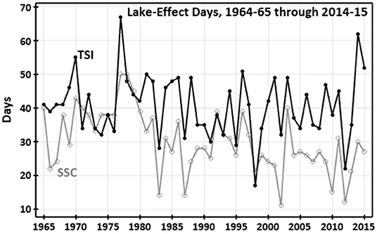
Figure 2. Seasonal number of lake-effect days for the eastern Great Lakes as determined by the TSI (black) and SSC (gray) methodologies.

Aside from TSI-based classifications (Ellis and Leathers, 1996; Karmosky, 2007; Suriano and Leathers, 2017a; Suriano et al., 2019), automated identification of regional lake-effect days to yield a usable historical data set is rare. Most recently, Hartnett (2021) identified snowstorms within the daily snowfall record of stations east of Lake Ontario, and used a manual scheme to classify each storm as directly associated with a mid-latitude cyclone or not. Storms not directly related to a cyclone, including lake-effect storms, were identified for the period 1985–2015. Given the manual nature of the classification methodology, the results are necessarily for a relatively small region of central New York state, and the storm classification data are not publicly accessible. Classification data from the two TSI-based studies that focus on lake-effect snowfall (Ellis and Leathers, 1996; Suriano and Leathers, 2017a) are not publicly accessible, nor are the data from the two studies that include lake-effect snowfall as an element of their classification results—study of the Catskill Mountains region of south-central New York state (Suriano et al., 2019) and study of the broader northeastern United States (Karmosky, 2007). At the opposite end of the temporal spectrum, case-study analyses of individual lake-effect storms or seasons abound (e.g., Kristovich et al., 2017).

The primary objective of this study is to present justified blends of the results of the TSI and SSC methodologies for identifying lake-effect days within the eastern Great Lakes region. Complementary analysis of the two lake-effect products aims to illustrate their differences, but rationalize their integration. The secondary purposes of the study are to characterize the lake-effect hydroclimate of the region through the study period using the blended datasets, and to render the full hybrid data set of historical lake-effect days accessible.

Materials and Methods

Comparative Analysis

The daily lake-effect calendars generated using the TSI and SSC methodologies were provided by the authors of the prior studies (Suriano and Leathers, 2017a; Ellis et al., 2021) and were aligned for comparison. Three groups of days are analyzed—the 742 lake-effect days identified as such by both methods, the 1,330 TSI lake-effect days unsupported by the SSC method, and the 794 SSC lake-effect days unsupported by the TSI method. TSI-only days are those for which the synoptic atmospheric flow suggests lake-effect, but air mass modification does not, while the opposite is the case for SSC-only days. From the TSI methodology, we chose not to include days from what Suriano and Leathers (2017a) deemed the “lake-enhanced” synoptic pattern, when moisture input from the lakes may have enhanced a mid-latitude weather system that produced precipitation on a broader scale.

We examined the 51-year time series of the annual fraction of lake-effect days for which the two methods agree and disagree for changes in the relationship between the two data sets through time, using Sen's slope estimator to calculate trend magnitude and the Mann-Kendall test to establish significance. We also segregated lake-effect days by month to identify dataset differences intra-seasonally. As the TSI yields multiple synoptic pattern types conducive to lake-effect precipitation, we determined the distribution of conflicting lake-effect days by TSI synoptic pattern to identify any obvious outlier in the level of agreement with the SSC methodology.

To assess disagreement between the two lake-effect data sets in terms of the synoptic atmosphere, we generated composites of sea-level pressure and 850 hPa air temperature from lake-effect days identified by both methods, and from lake-effect days identified by each method that were uncorroborated by the other method. North American Regional Reanalysis (NARR) data (Mesinger et al., 2006) were used to create gridded regional composites (~0.3° latitude × 0.3° longitude). The data were accessed through the United States Earth System Research Laboratory Physical Sciences Division's compositing platform (https://psl.noaa.gov/cgi-bin/data/narr/plotday.pl). We used the gridded composite data to create contour maps, focusing on the sea-level pressure pattern as the most distinct synoptic-scale variable associated with cool season lake effects (Ellis et al., 2021), but supplemented by 850 hPa air temperature when prudent, given its importance in the TSI-based methodology of Suriano and Leathers (2017a). A caveat is that NARR data extend back only to 1979, but we believe that the ~37-year record (January 1979 through April 2015) is of sufficient length for depicting mean atmospheric conditions, particularly given the advantage of a finer spatial resolution compared to other similar products of longer record.

We further evaluated the three sets of lake-effect days (TSI+SSC, TSI-only, and SSC-only) by portraying the magnitude and spatial pattern of precipitation frequency derived from the station-level Global Historical Climate Network (GHCN)-Daily database of the National Centers for Environmental Information (NCEI) (https://www.ncei.noaa.gov/products/land-based-station/global-historical-climatology-network-daily). All data within the GHCN-Daily database are subject to a suite of NCEI reviews before inclusion, forming one of the most complete repositories of in-situ precipitation data available (Menne et al., 2012). To focus on the area around the eastern Great Lakes, we identified 403 United States and Canadian stations within a region from 74° to 84° west longitude and from 39° to 46° north latitude (Figure 1). Requiring 90% data completeness for each of the three sets of lake-effect days reduced the number of stations to 298 (Figure 1). For each set of lake-effect days, the percentage of days with precipitation was calculated for each station, and the resulting station-level data were gridded to a resolution of ~0.5° latitude × 0.5° longitude grid to create mapped contours. The spatial pattern of precipitation frequency is most relevant for synoptic setup-defined lake-effect days (i.e., TSI-defined days), as the synoptic patterns are characterized as conducive to precipitation (Suriano and Leathers, 2017a). Still, a lake-effect spatial pattern depicted by the frequency of precipitation occurrence, even if weak, is anticipated to be evident for air mass modification-defined lake-effect days (i.e., SSC-defined days), despite their representation of air mass modification by the lakes rather than precipitation generation. The spatial pattern of precipitation frequency for each set of lake-effect days allows for an objective verification of lake effects across the different sets of days.

Hybrid Data Set Analysis

Results of the comparative analysis of the TSI- and SSC-based data sets supported their blending to create two hybrid data sets for analysis and dissemination. The “absolute” data set consists of days for which the methods agree are lake-effect days. The “hybrid” data set includes the days of agreement plus all days identified by one method but not the other, or what we term synoptic-defined (TSI, not SSC) and air mass modification-defined (SSC, not TSI). Replicating the approach of Ellis et al. (2021), we analyzed time series of lake-effect day occurrence graphically and with computation of the Sen's Slope estimator and Mann-Kendall significance test, while also testing the difference in the populations of lake-effect day frequency for the early and late halves of the record using a two-sample t-test. To portray the cool-season lake-effect hydroclimate across the region, we characterized station-level precipitation on lake-effect days using the array of GHCN-Daily stations. For each station, we computed mean seasonal lake-effect values of precipitation amount, precipitation frequency, and the percentage of seasonal precipitation and precipitation frequency attributed to lake-effect days. As outlined earlier, we gridded the derived data and generated mapped contours. Replicating the method of Ellis et al. (2021), we created mean regional values for each of the hydroclimate variables using 45 of the GHCN-Daily stations. The stations are within 160 km (100 mi) downwind of each of the lakes, and represent the 47 years 1968–69 through 2014–15 so to maximize station density per Ellis et al. (2021). To analyze hydroclimate change, we created time series of the mean regional values (annual seasonal means from the 45 stations) of each of the hydroclimatic variables and applied the aforementioned statistical tests for trend through the record and for difference between the temporal halves of the record.

Results

General Dataset Comparatives

When combined, the two methods yield 2,866 lake-effect days across the 51-year study period, for an average of about 56 per year, or about 31% of the 6-month season. The TSI method identified 2,072 lake-effect days, or an average of about 41 per year with a standard deviation of 9 days. The SSC method identified 1,536 days, or an average of about 30 days per year with a standard deviation of 9 days. The two methods agree on 742 days, or 35.8% of TSI lake-effect days and 48.5% of those identified by the SSC method. The annual frequencies of lake-effect days from the two methods covary, with a Pearson pairwise correlation value of 0.51 (p < 0.01). The percentage of annual lake-effect days (n = 2,866) for which the methods agree (n = 742) does not exhibit a statistically significant trend. The same is true when segregating the data into the sub-seasonal periods November (early-season), December through February (mid-season), and March/April (late-season), which align with the TSI seasons of Suriano and Leathers (2017a). Likewise, the percentage of TSI-defined lake-effect days (n = 2,072) supported by the SSC methodology (n = 742) is not characterized by a statistically significant trend, either seasonally or sub-seasonally. However, the percentage of SSC-defined lake-effect days (n = 1,536) supported by the TSI methodology (n = 742) exhibits a statistically significant positive trend, indicating increasing validation of SSC days by the TSI methodology. The magnitude of the trend is not large at +0.27 percent year⁻¹ (p = 0.02), amounting to approximately a 13% change over the course of the 51-year period. While a positive trend in early-season is somewhat evident (p = 0.10), the seasonal trend is largely a product of a positive trend of 0.24 percent year⁻¹ (p = 0.04) in mid-season. There is not a statistically significant trend for the late-season period.

Lake-effect days within one dataset uncorroborated by the other are temporally isolated within the lake-effect calendar. For the 1,330 TSI-defined lake-effect days that do not appear within the SSC data, 68.1% are not preceded or followed by another lake-effect day from either data set, and for only 8.2% of days is there an SSC-only day before or after. For the SSC data set, 77.8% of the 794 SSC-only lake-effect days do not have a lake-effect day from either data set preceding or following, and for only 6.3% of days is there a TSI-only day before or after. Thus, it does not appear that uncorroborated lake-effect days within either data set are commonly associated with a timing difference between data sets. Generally, the days of disagreement appear to be rather uniquely defined by each method.

Intra-seasonal differences between the TSI and SSC data sets are evident within the monthly climatology of lake-effect day frequency. While the percentage of seasonal lake-effect days occurring in mid-season are comparable between the two methods, the TSI method yields a much greater percentage of seasonal lake-effect days in the early-season period than does the SSC method (Table 1). The opposite is the case for the late-season period (March–April), when the percentage of seasonal lake-effect days generated by the SSC method is much greater than that for the TSI method (Table 1). So, while the TSI method yields more lake-effect days across all months than does the SSC, the two methods fundamentally differ in the shoulder periods of early- and late-season. This is made clear by the fraction of monthly lake-effect days within each data set that are corroborated by the other data set. For the TSI data, ~40% of lake-effect days in mid-season appear within the SSC data set, and about 35% for the late-season period, but only 19% during the early-season (Table 1). For the SSC data, about 60% of lake-effect days in November, January, and February appear in the TSI data set, 50% in December, but only 14% in March and 4% in April (Table 1). When the data sets are combined into one record, the percentage of days for which the methods corroborate one another ranges from about 30 to 34% in mid-season, but declines to 17% in early-season, and 11% and 4% in the late-season months of March and April (Table 1). Of the 742 lake-effect days upon which the two methods agree, 620 (84%) are within mid-season.

TABLE 1

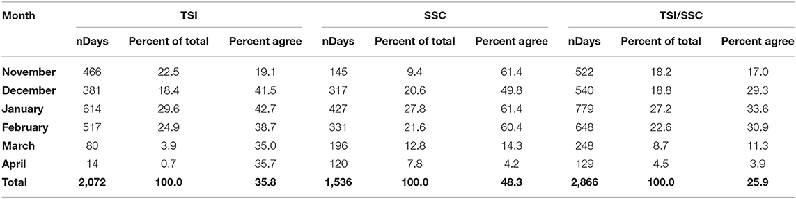
Table 1. For lake-effect days identified by the TSI method, SSC method, and the methods combined (TSI/SSC), the monthly distribution, the percentage of seasonal days occurring within each month, and the percentage of days each month that are supported by the other method (TSI, SSC), or by both methods (TSI/SSC), 1964–65 through 2014–15.

Uncorroborated TSI Data

The greatest number of uncorroborated TSI-defined lake-effect days is in mid-season (December–February), when the rate of corroboration is actually greatest, but the frequency of lake-effect days is also greatest. Conversely, the early-season (November) has the lowest rate of corroboration, yielding a relatively large number of days not supported by the SSC data. There are few TSI-defined lake-effect days in late-season (March–April), with a corroboration rate rivaling that of mid-season, possibly owing simply to a high frequency of SSC-defined lake-effect days in spring relative to the low frequency within the TSI dataset.

There is very little difference in the mean sea-level pressure pattern for TSI-defined lake-effect days corroborated by SSC data (Figures 3A–C) and those uncorroborated (Figures 3D–F). The classic lake-effect pattern, with a high-pressure center over the central United States and a low-pressure center along the northeastern coastline of North America, is evident for the early- and mid-seasons. In late-season, the high-pressure center is located farther north, while the low-pressure center is farther south, imparting a more north-to-south flow across the eastern Great Lakes than the northwest-to-southeast orientation earlier in the season. However, this pattern is specific to the single TSI synoptic atmospheric setup judged by Suriano and Leathers (2017a) as conducive to lake-effect snowfall in spring. Across the 6-month season it does not appear that uncorroborated TSI-defined lake-effect days are associated with a mean sea-level pressure pattern that is noticeably different from that associated with corroborated days. A feature more subtle than synoptic-scale sea-level pressure, such as lower-atmospheric temperature, appears to prevent the SSC methodology from matching these TSI-defined lake-effect days.

FIGURE 3

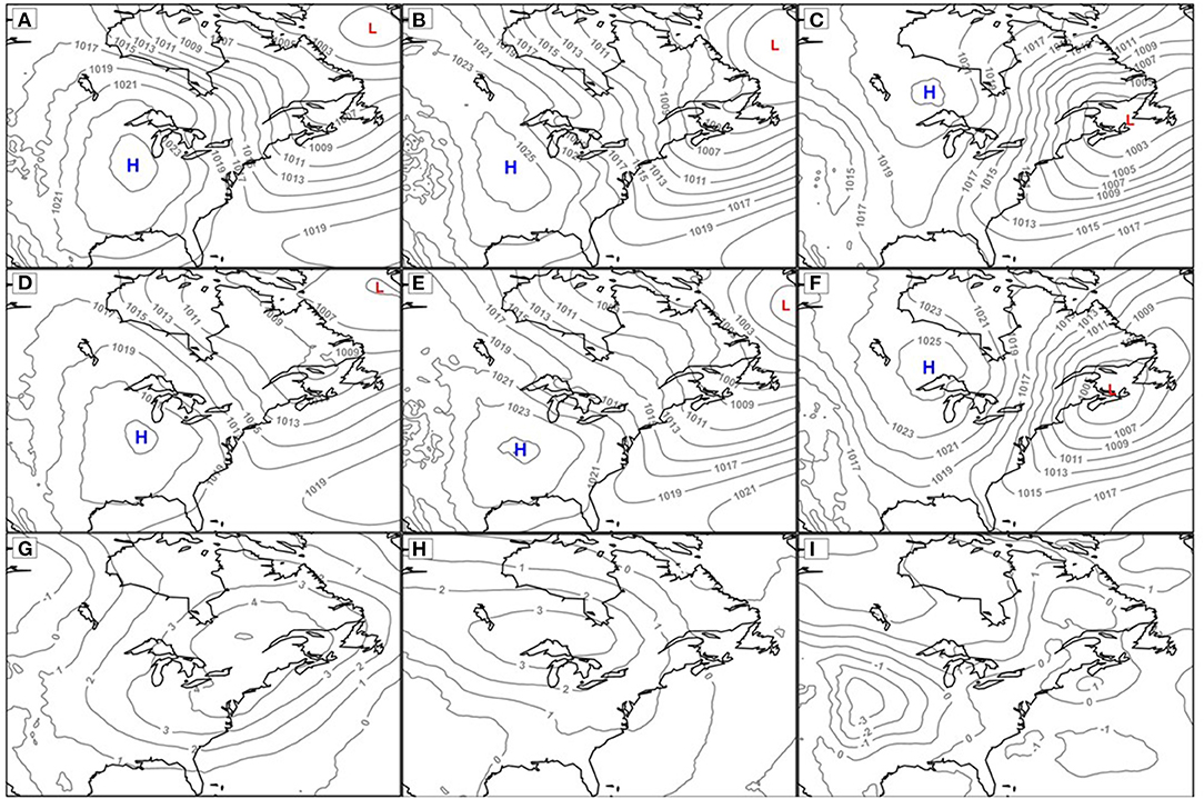
Figure 3. For TSI-defined lake-effect days in early-season (left column), mid-season (middle column), and late-season (right column), mean sea-level pressure (hPa) for days corroborated by SSC data (A–C), mean sea-level pressure for uncorroborated days (D–F), and difference in mean 850 hPa air temperature (°C) on uncorroborated and corroborated days (uncorroborated minus corroborated) (G–I), 1964–65 through 2014–15. Isobars are in 2-hPa intervals, and air temperature differences are in 1°C intervals.

In their identification of TSI synoptic patterns conducive to lake-effect snowfall, Suriano and Leathers (2017a) based their decisions on several characteristics, the most fundamental being mean sea-level pressure pattern and mean lake surface-to-850 hPa air temperature. By using mean values of variables such as air temperature, it is possible that a synoptic type deemed conducive to lake-effect snowfall includes days that are more marginal than others, enough so that they could be days that the SSC methodology failed to identify. Lending some credence to this is the difference in 850 hPa air temperature between TSI-defined lake-effect days that are corroborated and uncorroborated by SSC data. For November, the mean 850 hPa air temperature for uncorroborated days is more than 4°C warmer than for corroborated days, while for December through February the difference is >2°C (Figures 3G,H). The greater mean temperatures on uncorroborated TSI-defined lake-effect days suggest that they are the warmer days within the population of days of each of the lake-effect TSI types for November and December through February. This is not the case for March and April, as there is little difference in mean 850 hPa air temperature for corroborated and uncorroborated TSI-defined lake-effect days (Figure 3I).

The element of the SSC definition that prevents corroboration of TSI-defined lake-effect days supports the idea that the intensity of cold air across the region may be a source of methodological disagreement during the early-season. There are three geographic regions for which SSC weather types are examined, together, for determination of a lake-effect day (Ellis et al., 2021). Using four stations immediately east (downwind) of the eastern lakes (Figure 1), at least one station must be of the moist-polar (MP) or transition (TR) (onset or demise of lake-effects) weather type, and all others of the dry-polar (DP) type. Within a region north (upwind) of the eastern lakes (Figure 1), at least two of four stations must be of the dry-polar (DP) weather type. Lastly, within a region along the northeastern United States coastline (well-downwind) (Figure 1), at least two of four stations must be of the dry-polar (DP) or transition (TR) (cold front passage) weather type. If the criterion of any one region fails, the day is identified as a non-lake-effect day. For the 1,330 TSI-defined lake-effect days not identified as such by the SSC methodology, there are a total of 2,124 causes of failure among the three regions used to define an SSC lake-effect day, of which 39.5% stem from the lake-effect region, 31.2% from the northern region, and 29.3% from the eastern region. While a polar weather type is a requirement for all three regions (expansive cold air), the lake-effect region also requires evidence of a lake influence on humidity [moist-polar (MP)], whereas the presence of cold, dry air is the primary criterion in the northern and eastern regions. When segregating the causes of failure to corroborate a TSI-defined lake-effect day by month, the proportion attributed to the lake-effect region increases through the season, while that for the northern and eastern regions decreases through the season. This pattern is even more pronounced when focusing on the instances for which the criterion in only one region caused the failure of the SSC to corroborate a TSI-defined lake-effect day, which is to say, those days that were very close to meeting the SSC definition. Out of 586 such cases (44.1% of 1,330 TSI-only lake-effect days), 47.1% stemmed from the lake-effect region, 29.9% from the northern region, and 23% from the eastern region. The attribution of monthly instances to the lake-effect region increases through the season, while those attributed to the northern and eastern regions decrease through the season.

It appears that violating the cold air requirement within the eastern and northern regions of the SSC methodology on TSI-defined lake-effect days is more likely during the first half of the season, becoming much less likely in late-season. The lack of sufficiently cold air is also likely the case for definition violations stemming from the lake-effect region, but lack of a lake-effect in the form of increased humidity contributes, likely producing the greater fraction of definition violations later in the season. These patterns are logical, as marginally-cold air masses passing over the lakes are more likely in the warmer early portion of the season, and marginally-humidified air through interaction with the lakes is more likely late in the season due to reduced lake temperatures and ice cover. However, the propensity for more early-season violations of the SSC methodology on TSI-defined lake-effect days may also stem from the humidity aspect of the cold, dry air requirement at the SSC stations north of the lakes.

For lake-effect days identified by both methods, the percentage of days with precipitation across the region is greatest, spatially, to the lee of the eastern lakes in early-season (60–70%) (Figure 4A), mid-season (60–70%) (Figure 4B), and late-season (50–70%) (Figure 4C). For TSI-defined days uncorroborated by SSC data, slightly smaller percentages (50–60%) are evident to the lee of the lakes in early-season (Figure 4D) and mid-season (Figure 4E). The contrast is greater for uncorroborated days in late-season—only about 30–40% of the days are characterized by precipitation to the lee of the lakes (Figure 4F). For the TSI-defined days that are uncorroborated by SSC data, slightly higher percentages of days with precipitation are evident in the region north of the eastern Great Lakes in early-season (Figure 4D) and mid-season (Figure 4E), compared to days corroborated by SSC data (Figures 4A,D). This is not the case in late-season (Figure 4F). Days with precipitation in this area north of the lakes, possibly associated with the departing low-pressure center to the northeast (Figures 3D,E) or sourced from the western lakes, are likely classified as something other than the dry-polar (DP) weather type by the SSC methodology, violating the SSC-based definition of a lake-effect day.

FIGURE 4

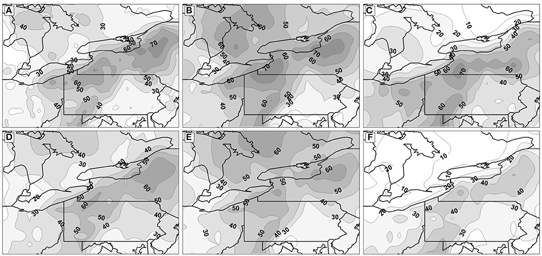
Figure 4. Percentage of lake-effect days with precipitation in early-season (left column), mid-season (middle column), and late-season (right column) for days identified by both TSI and SSC methods (A–C), and for TSI-defined days uncorroborated by SSC data (D–F), 1964–65 through 2014–15. Contours are in 10% intervals.

As the TSI methodology generalizes the atmospheric pattern for the region using conditions at one station, and also generalizes the conduciveness for lake-effect snowfall based on the mean lower-atmospheric characteristics of each synoptic pattern type and mean monthly lake temperature, it is reasonable to believe that some days within a TSI synoptic type do not satisfy the criteria established by Suriano and Leathers (2017a). This is not to say that these are exclusively the days that lack corroboration by the SSC method, as the SSC method is limited and aims at a slightly different objective. Further, of the 1,330 TSI-defined lake-effect days that do not appear in the SSC data for the eastern lakes, 454 (34%) were classified as western lakes lake-effect days within the SSC methodology (Ellis et al., 2021), adding credence to those TSI-defined lake-effect days. While the results here help to rationalize the uncorroborated TSI-defined lake-effect days, they neither explicitly confirm nor deny that they should be included in the TSI-defined lake-effect data set.

Uncorroborated SSC Data

While the TSI methodology yields a greater number of lake-effect days than are within the SSC data set, there are 794 SSC-defined days that do not appear in the TSI data set. Most (455 days, or 57.3%) are in mid-season (December–February), while the fewest are in early-season (November) (56 days, or 7.1%), when the SSC method yields a much smaller proportion of seasonal lake-effect days than does the TSI method. The opposite is true in late-season (March–April), when a much greater fraction of seasonal SSC-defined days occurs relative to the TSI dataset. As such, 35.6% (283 days) of the SSC-defined lake-effect days not corroborated by TSI data occur during the late-season.

While Suriano and Leathers (2017a) defined only seven TSI synoptic atmospheric patterns as conducive to lake-effect snowfall, the 794 SSC-defined lake-effect days uncorroborated by TSI data are distributed across 28 other TSI types. Of the six types that each account for at least 5% of the 794 days, four are mid-season TSI types and two are spring types. Of the other 22, nine each account for <1% of the days. The mean sea-level pressure patterns from the 56 SSC-defined lake-effect days in early-season that are uncorroborated by TSI data (Figure 5A) and the 455 days in mid-season (Figure 5B) are broadly typical of that for lake effects (e.g., Figures 3A,B), except that the center of high-pressure is not optimally positioned to foster strong low-level cold-air advection across the Great Lakes region. This is evident in the weak sea-level pressure gradient across the eastern lakes within the composites. The patterns apparently support the necessary expanse of the dry-polar (DP) weather type required by the SSC methodology, but lake-effects are likely subtler under these patterns—enough to yield the moist-polar (MP) and/or transition (TR) weather types within the lake-effect region, but likely not enough to generate snowfall per the objective of the TSI method. For the 283 SSC-defined lake-effect days in late-season not supported by the TSI data, the mean sea-level pressure pattern (Figure 5C) closely resembles that for days in which the methods agree (Figure 3C), although with a weaker gradient across the eastern lakes. Given the similar pattern, and the lack of lake-effect days generated by the TSI method in late-season, it is most likely that cooler lakes and greater ice coverage is enough to limit lake-effect snowfall (TSI) despite some modification of the passing lower-atmosphere (SSC).

FIGURE 5

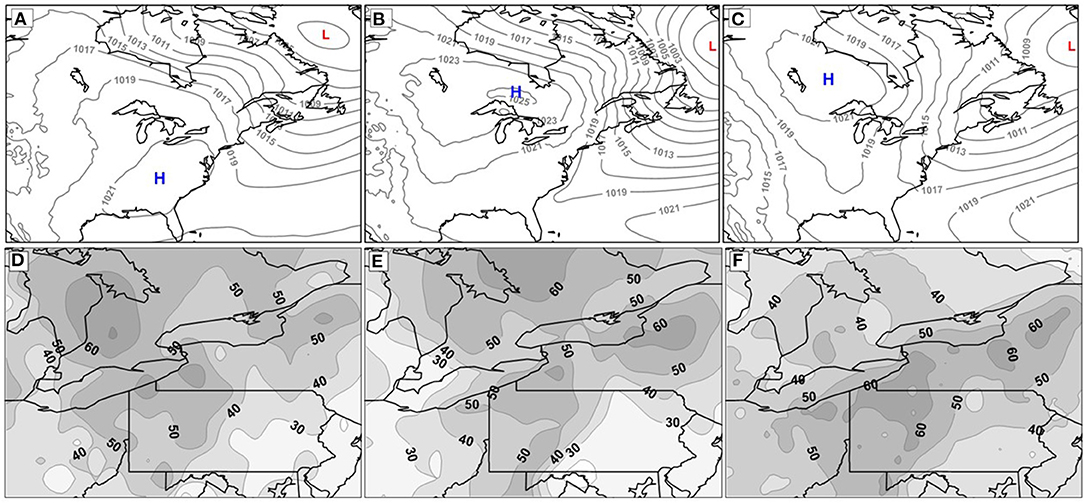
Figure 5. Mean sea-level pressure (hPa) (A–C) and percentage of days with precipitation (D–F) for SSC-defined lake-effect days in early-season (left column), mid-season (middle column), and late-season (right column) uncorroborated by the TSI data set, 1964–65 through 2014–15. Isobars are in 2-hPa intervals, and percentage contours are in 10% intervals.

Aligning with the sea-level pressure patterns are the percentages of uncorroborated SSC-defined lake-effect days with precipitation. For early-season (Figure 5D) and mid-season (Figure 5E), values west of the eastern lakes, while relatively small, are comparable to those to the east of the lakes. This is presumably due to the relatively weak flow of cold air across the region (Figures 5A,B), yielding a subtler lake effect (modified air) without the unidirectional nature of classic lake-effect precipitation. The more typical lake-effect pressure pattern in late-season (Figure 5C) aligns with higher precipitation percentages in the traditional lake-effect areas south and east of the eastern lakes (Figure 5F), although values to the west of the lakes remain relatively high compared to SSC days corroborated by TSI data (Figure 4C).

As with uncorroborated TSI-defined lake-effect days, there is not convincing evidence for declassifying the lake-effect days within the SSC data set that are not among those in the TSI data. Rather, their intra-seasonal distribution and the combination of their mean synoptic-scale atmospheric pressure pattern and predominant precipitation pattern seem to illustrate the different objective of the SSC method compared to the TSI method. This makes integration of their results for a more thorough representation of historical daily lake-effects reasonable.

Merged Data

In combining the two lake-effect data sets, we chose to honor the objective of each of the methodologies by retaining all days within each, creating one “absolute” and one “hybrid” data set. Absolute data are only days identified by both methods, or what are likely the most obvious occurrences of lake-effects. Supporting the idea that absolute days are most robust is the lesser degree to which they are temporally isolated. Whereas, only 31.9 and 22.2% of TSI-only days and SSC-only days, respectively, are preceded or followed by a lake-effect day of any type, 54.8% of absolute lake-effect days are preceded or followed by a lake-effect day. Added to the absolute lake-effect days to create the hybrid data set are days identified by one method that are uncorroborated by the other method. In other words, the hybrid data set consists of days of agreement, TSI-only days, or what we term “synoptic setup” days, and SSC-only days, or what we term “air mass modification” days.

Seasonally, absolute lake-effect days average 14–15 per year, exhibiting an insignificant decline of −0.8 days decade⁻¹ (p = 0.09) (Figure 6a), and averaging nearly 16 days per season through the first 25 years of the record and about 13 days per season over the final 25 days of the record. On average, 26 synoptic setup-defined days occur each season (Figure 6b), while only 15–16 air mass modification-defined days occur each year, but with a statistically significant decline of 2.3 days decade⁻¹ (p < 0.01) (Figure 6c). Two-sample t-test results illustrate a significant difference (p < 0.01) between the occurrence of air mass modification days during the first 25 years (mean = 18 days) and final 25 years (13 days) of the record. The cumulative expression of the three sets of data, the hybrid data set, averages about 56 days per year, but with a statistically significant decline in frequency over the study period of 2.8 days decade⁻¹ (p < 0.01) that appears most pronounced from the late-1970s through the early-2000s (Figure 6d). Over the first 25 years of the record, the hybrid data set averages about 60 days per year, while averaging only 52 days per year over the final 25 years of the record (two-sample t-test p < 0.01).

FIGURE 6

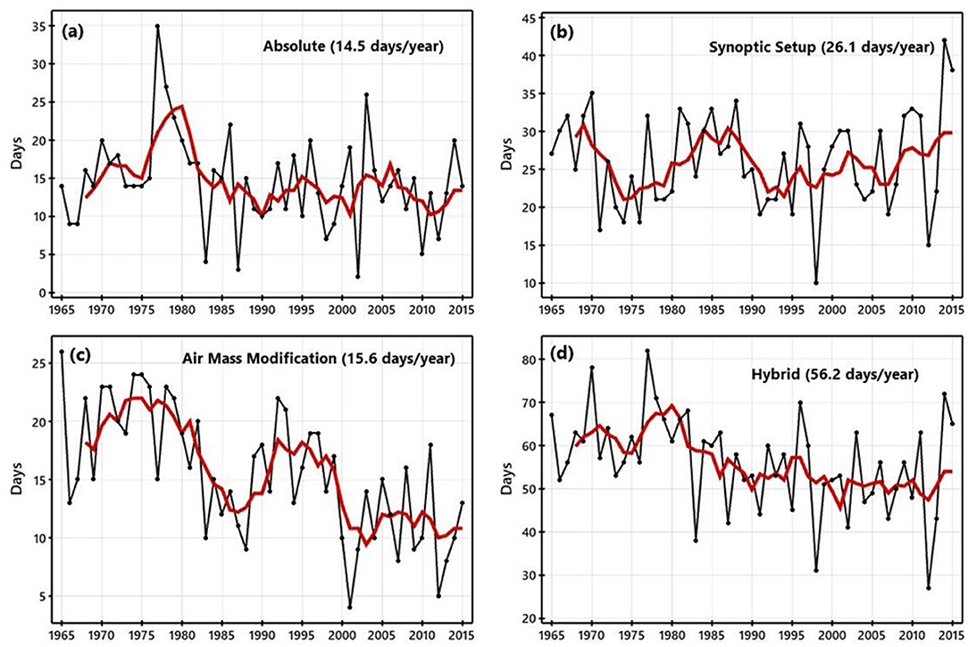
Figure 6. Time series of seasonal lake-effect frequency (days) for absolute lake-effect days (a), synoptic setup-defined days (b), air mass modification-defined days (c), and for the three classes combined (hybrid) (d) for the period 1964–65 through 2014–15. The red line is a 5-year running mean. The period of record annual mean for each is indicated.

Focusing on the hybrid data set, the mean amount of seasonal precipitation attributed to lake-effect days ranges from about 120–160 mm east of Lake Erie, and 120–220 mm east of Lake Ontario (Figure 7A). The mean seasonal frequency of precipitation follows a similar spatial pattern, with values from 25 to 30 days east of Lake Erie and 30–35 days east of Lake Ontario (Figure 7B). The mean percentage of total seasonal precipitation attributed to lake-effect days ranges from 25 to 30% east of Lake Erie, and is about 30% to the north, east of Lake Ontario (Figure 7C). Similarly, the mean percentage of total seasonal precipitation frequency attributed to lake-effect days is about 35% to the east of each of the lakes (Figure 7D). Values attributed to the absolute data set (not shown) follow the same spatial patterns, but obviously of much smaller magnitudes, given the much smaller population of absolute lake-effect days compared to hybrid days.

FIGURE 7

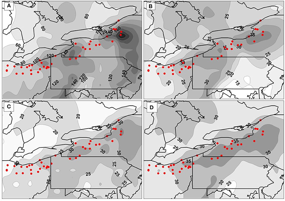
Figure 7. Station-level values of mean seasonal precipitation (liquid; mm; 20 mm intervals) (A), precipitation frequency (days; 5-day intervals) (B), percentage of seasonal precipitation (liquid; 5% interval) (C), and percentage of seasonal precipitation frequency (5% interval) (D) associated with the lake-effect days of the hybrid data set, 1964–65 through 2014–15. Red dots indicate locations of stations used to calculate regional values.

Calculated from the 45 lake-effect stations to the lee of the lakes (Figure 7), regional mean seasonal values of precipitation characteristics attributed to days within the hybrid data set generally exhibit a decline over the 47-year period 1968–69 through 2014–15 (Figure 8). This is despite no change in total seasonal precipitation (all days, regardless of lake effect)—small, statistically insignificant increases in both precipitation and precipitation frequency. For the region, mean seasonal precipitation (liquid amount) on days within the hybrid data set declined at a rate of 7.8 mm decade⁻¹ (p = 0.02), while also appearing to become more variable in recent years (Figure 8a). However, a two-sample t-test reveals no statistically significant difference in seasonal precipitation during the first (mean = 124 mm year⁻¹) and last (mean = 119 m year⁻¹) 23 years of the record. So, while a trend is present, the broad change in precipitation is not significant. Likewise, a decline in regional mean seasonal precipitation frequency within the hybrid data set (−1.3 days decade⁻¹) (Figure 8b) is statistically significant (p = 0.04), but the frequency for the early years (mean = 29 days year⁻¹) is not statistically significantly different than the frequency for the late years (mean = 26 days year⁻¹). More evident are changes in the percentage of seasonal precipitation and precipitation frequency attributed to days within the hybrid data set. The mean regional fraction of seasonal precipitation (Figure 8c) decreased at a rate of 2.2 percent decade⁻¹ (p < 0.01), but values from the early and late portions of the record are not statistically significantly different [mean = 26% year⁻¹ early, 23% year⁻¹ late (p = 0.10)]. However, for the percent of seasonal precipitation frequency (Figure 8d), both the trend (−2.0 percent decade⁻¹, p < 0.01) and the difference in early and late values [mean = 33% year⁻¹ early, 29% yr⁻¹ late (p = 0.03)] reflect statistically significant declines. Within the absolute data set, none of the variables exhibited a statistically significant change. This is not surprising, given the rather small values and limited variability within the data (Figure 8).

FIGURE 8

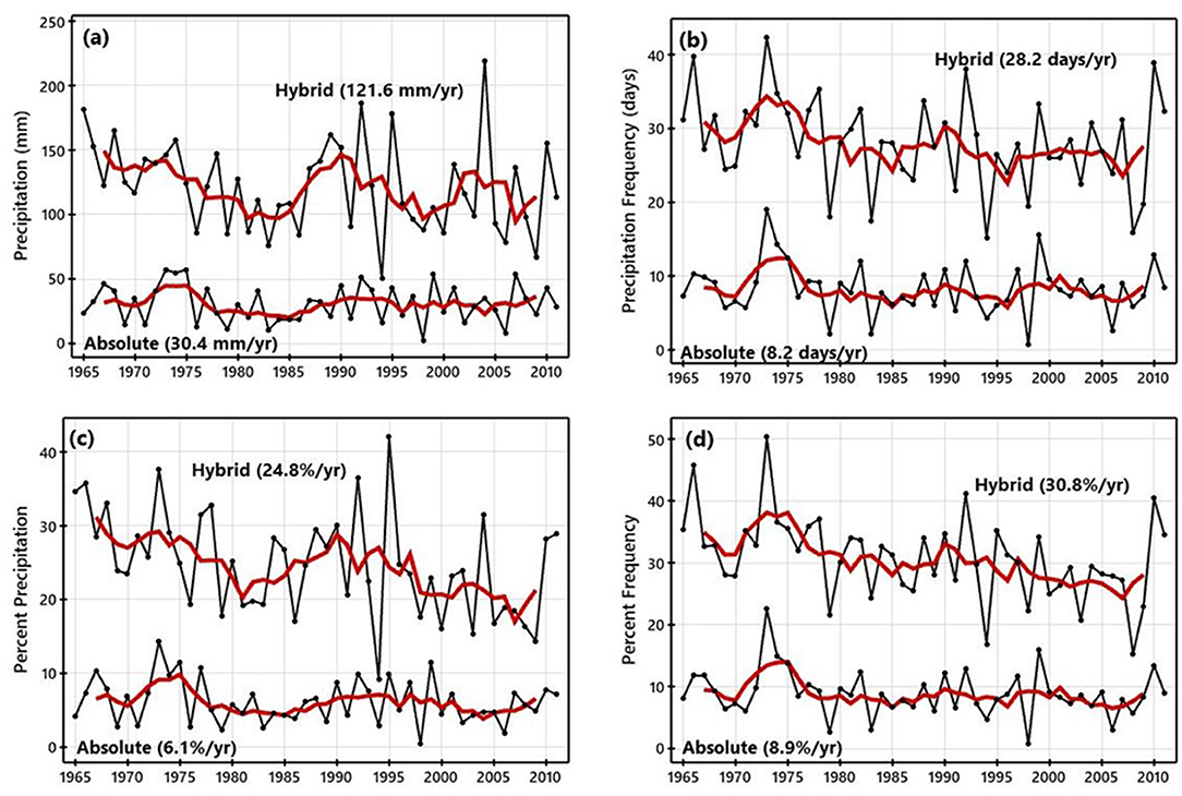
Figure 8. For the 45 precipitation stations (Figure 7), regional mean seasonal values of precipitation (a), precipitation frequency (b), percent of seasonal precipitation (c), and percent of seasonal precipitation frequency (d) attributed to days within the hybrid and pure data sets for the period 1968–69 through 2014–15.

Discussion

The two methods for identifying lake-effect days within the historical record differ in the degree of the lake-effect that they aim to recognize. The TSI method is designed to find days with a broad synoptic-scale pattern that yields strong, cold flow across the Great Lakes region conducive to lake-effect snowfall. The SSC-based method aims to identify days with a signature of air mass modification by the lakes, such that a broad cold, dry air mass across the greater region contains cold, moist air specifically within the traditional lake-effect areas. While the methods overlap, the TSI method likely finds additional days with stronger atmospheric dynamics that yield a regional arrangement of air masses that may not fit the ideal lake-effect model, while the SSC method likely finds additional days with weaker dynamics and a subtler lake effect that may not yield a profound weather impact. We submit that combining the two data sets yields a more thorough record of daily instances of lake-effects from Lakes Erie and Ontario for the cool seasons 1964–65 through 2014–15.

Two main caveats accompany the merged data. The first is the trend toward increasing validation of SSC-defined lake-effect days by the TSI method, particularly in mid-season. This coincides with a trend toward fewer SSC-defined lake-effect days in recent decades (Ellis et al., 2021), possibly indicating that the frequency trend partly reflects a decline in more marginal lake-effect days as defined by the SSC method—those not supported by the TSI method. Otherwise, there is not an obvious explanation for the trend, as neither methodology was applied differently through the record, and the quality of the input data for each methodology should not have changed gradually through time. While merely speculative, it is possible that the pervasive warming of recent years is enough for the SSC methodology to increasingly classify a day as of a moderate weather type rather than a polar type (i.e., dry-moderate/moist-moderate rather than dry-polar/moist-polar). This would impact the methodology for establishing SSC-defined lake-effect days, possibly shedding marginal days (moderate rather than polar) so to increase the fraction validated by the TSI method. To investigate this theory would require intensive analysis of the mechanics of the SSC methodology, which is beyond the scope of this study. However, this is a caution, or possibly a limitation, accompanying the data set.

The second caveat with the merged data is the greater discrepancy between the two contributing data sets within the shoulder periods of the November through April season than during mid-season. The rationale for the greater frequency of SSC-defined lake-effect days in late-season (March/April) relative to the few TSI-defined days is rather clear. By late-season, lake temperatures have lowered and ice-coverage has increased, making the generation of lake-effect snowfall more difficult, which is realized in fewer TSI-defined lake-effect days. However, lake-influence is quite possibly great enough to raise the humidity of the passing cold, dry air and influence the weather type within the SSC data set to yield an SSC-defined lake-effect day. Less clearly rationalized is the greater frequency of TSI-defined lake-effect days in early-season (November) relative to the fewer SSC-defined days. As indicated by the comparative analysis of the data sets, it seems probable that while a synoptic flow pattern in November suggests lake-effect (TSI), the cold air may be more marginal (i.e., moderate, rather than dry-polar or moist-polar), in magnitude and/or spatial extent, so to not satisfy the SSC definition. Ellis et al. (2021) considered the possibility of the lakes modifying air temperature enough to alter the dry-polar weather type upstream to the moist-moderate weather type downstream, rather than the moist-polar type, as required by the SSC methodology. However, they did not choose to implement weather type modification based on air temperature within their methodology.

The hybrid data set produced here yields seasonal values of lake-effect frequency and precipitation that align well with previously published estimates. As a merger of the data sets produced by Suriano and Leathers (2017a) and Ellis et al. (2021), there is greater meaning from a comparison with the results of other studies. In developing a method for classifying snowstorm types for an area east of Lake Ontario, Hartnett (2021) found lake-effect snowstorms to account for 35% of snowstorms, yielding ~24 lake-effect snowfall days per year and 39% of seasonal snowfall for the period 1985–2015. This compares well with mean regional values from the hybrid data set – 30-35 lake-effect precipitation days per year that account for about 30% of seasonal liquid total precipitation (in all forms), the latter of which maximizes at about 35% across the area of Hartnett's study. Karmosky (2007) attributed ~35% of seasonal snowfall immediately east of eastern lakes to lake effects, declining to <25% when ~100 km inland. Suriano et al. (2019) determined that an average of 28 lake effect days per year produce 38% of seasonal total snowfall farther east in the Catskill Mountains region well to the east of Lake Ontario. The declining trend in lake effects from the late 1970s through the early 2000s portrayed by the hybrid data set matches the findings of several studies (e.g., Hartnett et al., 2014; Suriano and Leathers, 2017b; Ellis et al., 2021). Given the historical prominence of lake-effect precipitation within the cool-season hydroclimate of the region, a continued decline in the frequency of lake effects, or even the establishment of the lower frequency as a new normal, has acute implications for the regional hydroclimate.

The merged data, we believe, can serve further research efforts focused on the lake effects of the eastern Great Lakes. Forecasting lake-effect precipitation, either seasonally or for individual events, remains challenging, and the impact of a changing climate on the role of lake-effects within the regional hydroclimate is complex. The calendars of hybrid and absolute lake-effect days merged from the two methodologies provide a more comprehensive collection of lake-effect days for analysis of any form. To serve pursuit of a better understanding of lake effects in the region, the hybrid, absolute, synoptic setup-defined, and air mass modification-defined lake-effect calendars are available through the University Libraries data portal of Virginia Tech (https://doi.org/10.7294/16712872).

Data Availability Statement

The datasets presented in this study can be found in online repositories. The names of the repository/repositories and accession number(s) can be found below: https://doi.org/10.7294/16712872.

Author Contributions

AE and ZS collaboratively developed the design for this study and authored elements of the manuscript. ZS conducted initial comparative analysis of TSI lake-effect data with SSC data, while AE conducted initial comparative analysis of SSC lake-effect data with TSI data. AE constructed synoptic composites and conducted climatological precipitation analyses. All authors contributed to the article and approved the submitted version.

Conflict of Interest

The authors declare that the research was conducted in the absence of any commercial or financial relationships that could be construed as a potential conflict of interest.

Publisher's Note

All claims expressed in this article are solely those of the authors and do not necessarily represent those of their affiliated organizations, or those of the publisher, the editors and the reviewers. Any product that may be evaluated in this article, or claim that may be made by its manufacturer, is not guaranteed or endorsed by the publisher.

Acknowledgments

The authors acknowledge Mr. Reggie Wortman, University of Nebraska Omaha, for help with data access and distillation.

References

Andresen, J. A. (2012). “Historical climate trends in Michigan and the Great Lakes region,” in Climate Change in the Great Lakes Region, eds. T. Dietz and D. Bidwell (Lansing, MI: Michigan State University Press), 17–34.

Ellis, A. W., and Leathers, D. J. (1996). A synoptic climatological approach to the analysis of lake-effect snowfall: potential forecasting applications. Weather Forecast. 11, 216–229. doi: 10.1175/1520-0434(1996)011<0216:ASCATT>2.0.CO;2

CrossRef Full Text | Google Scholar

Ellis, A. W., Marston, M. L., and Bahret, J. (2021). Changes in the frequency of cool season lake effects within the North American Great Lakes region. Ann. Am. Assoc. Geogr. 111, 385–401. doi: 10.1080/24694452.2020.1785270

CrossRef Full Text | Google Scholar

Hartnett, J. J. (2021). A classification scheme for identifying snowstorms affecting central New York State. Int. J. Clim. 15, 1712–1730. doi: 10.1002/joc.6922

CrossRef Full Text | Google Scholar

Hartnett, J. J., Collins, J. M., Baxter, M. A., and Chambers, D. P. (2014). Spatiotemporal snowfall trends in central New York. J. Appl. Meteor. Clim. 53, 2685–2697. doi: 10.1175/JAMC-D-14-0084.1

CrossRef Full Text | Google Scholar

Holroyd, E. W. III. (1971). Lake effect cloud bands as seen from weather satellites. J. Atmos. Sci. 28, 1165–1170. doi: 10.1175/1520-0469(1971)028<1165:LECBAS>2.0.CO;2

CrossRef Full Text | Google Scholar

Kalkstein, L. S., and Corrigan, P. (1986). A synoptic classification approach for geographical analysis: assessment of sulfur dioxide concentrations. Ann. Assoc. Am. Geogr. 76, 381–395. doi: 10.1111/j.1467-8306.1986.tb00126.x

CrossRef Full Text | Google Scholar

Karmosky, C. (2007). Synoptic Climatology of Snowfall in the Northeastern United States: An Analysis of Snowfall Amounts From Diverse Synoptic Types. Master's Thesis, University of Delaware, Newark, DE. Available at: ProQuest Dissertations and Theses Global. (304860693). Retrieved from: http://login.ezproxy.lib.vt.edu/login?url=https://www.proquest.com/dissertations-theses/synoptic-climatology-snowfall-northeastern-united/docview/304860693/se-2?accountid=14826 (accessed September 17, 2021).

Google Scholar

Kristovich, D. A. R., Clark, R. D., Frame, J., Geerts, B., Knupp, K. R., Kosiba, K. A., et al. (2017). The Ontario winter lake-effect systems campaign: scientific and educational adventures to further our knowledge and prediction of lake-effect storms. Bull. Am. Meteorol. Soc. 98, 315–332. doi: 10.1175/BAMS-D-15-00034.1

CrossRef Full Text | Google Scholar

Menne, M. J., Durre, I., Vose, R. S., Gleason, B. E., and Houston, T. G. (2012). An overview of the Global Historical Climatology Network-Daily Database. J. Atmos. Oceanic Technol. 29, 897–910. doi: 10.1175/JTECH-D-11-00103.1

CrossRef Full Text | Google Scholar

Mesinger, F., Dimego, G., Kalnay, E., Mitchell, K., Shafran, P. C., Ebisuzaki, W., et al. (2006). North American regional reanalysis. Bull. Am. Meteorol. Soc. 87, 343–360. doi: 10.1175/BAMS-87-3-343

CrossRef Full Text | Google Scholar

Notaro, M., Holman, K., Zarrin, A., Vavrus, S., and Bennington, V. (2013). Influence of the Laurentian Great Lakes on regional climate. J. Clim. 26 789–804. doi: 10.1175/JCLI-D-12-00140.1

CrossRef Full Text | Google Scholar

Scott, R. W., and Huff, F. A. (1996). Impacts of the Great Lakes on regional climate conditions. J. Great Lakes Res. 22, 845–863. doi: 10.1016/S0380-1330(96)71006-7

CrossRef Full Text | Google Scholar

Sheridan, S. C. (2002). The redevelopment of a weather-type classification scheme for North America. Int. J. Clim. 22, 51–68. doi: 10.1002/joc.709

CrossRef Full Text | Google Scholar

Suriano, Z. J., and Leathers, D. J. (2017a). Synoptic climatology of lake-effect snowfall conditions in the eastern Great Lakes region. Int. J. Clim. 37, 4377–4389. doi: 10.1002/joc.5093

CrossRef Full Text | Google Scholar

Suriano, Z. J., and Leathers, D. J. (2017b). Synoptically classified lake-effect snowfall trends to the lee of Lakes Erie and Ontario. Clim. Res. 74, 1–13. doi: 10.3354/cr01480

CrossRef Full Text | Google Scholar

Suriano, Z. J., Leathers, D. J., Hall, D. K., and Frei, A. (2019). Contribution of snowfall from diverse synoptic conditions in the Catskill/Delaware Watershed of New York State. Int. J. Clim. 39, 3608–3618. doi: 10.1002/joc.6043

PubMed Abstract | CrossRef Full Text | Google Scholar