Abstract
The response of regional climate models (RCMs) to different input land cover information is complex and uncertain. Several studies by the regional climate modeling community have investigated the potential of land cover data to help understand land-atmosphere interactions at regional and local scales. This study investigates the regional climate response to introducing European Space Agency (ESA) land cover (LC) data into WRF-Hydro. In addition, this study assesses the potential impacts of afforestation and deforestation strategies on regional water and energy fluxes. An extended version of WRF-Hydro that accounts for a two-way river-land water flow to reduce unrealistic peaks in simulated discharge was employed. The two-way river-land flow setup yielded a better NSE and KGE of 0.47 and 0.69, respectively, over the Kulpawn basin compared to the default setup values of −0.34 and 0.2. Two land use/land cover change effects were deduced from synthetic numerical sensitivity experiments mimicking afforestation by closed shrubland expansion and deforestation by cropland expansion. The afforestation experiment yielded approximately 6% more precipitation, 3% more evapotranspiration, 27% more surface runoff, and 16% more underground runoff, while the deforestation by cropland expansion yielded −5% less precipitation, −3% less evapotranspiration, −3% less surface runoff, and − 9% less underground runoff over the Sissili-Kulpawn Basin (SKB). This result suggests that afforestation (deforestation) could increase the flood (drought) risk. Our synthetic numerical experiment mimics the regional water and energy budgets well and can help climate services and decision-makers by quantifying regional climate response to potential land cover changes.
1 Introduction
Anthropogenic land use and land cover changes such as deforestation, afforestation, and agricultural practices have been long established to have climatic effects (Feddema et al., 2005; Foley et al., 2005; Bonan, 2008; Mortey et al., 2023) through the change of land surface properties. A change in land surface properties will directly affect the land-atmosphere interactions and consequently alter the dynamic and thermodynamic characteristics resulting in different climatic patterns and processes (Deng et al., 2014). Changes in the land surface could lead to changes in biogeophysical parameters [e.g., albedo (), leaf area index (LAI)] which alter radiative fluxes (e.g., outgoing longwave radiation) and ultimately perturb surface moisture- and energy budgets. Land surface albedo directly alters the incoming solar radiation absorbed by a surface, subsequently leading to a change in outgoing longwave radiation and the energy available for the earth’s surface (Feddema et al., 2005). Vegetation transpiration and surface hydrology determine how the energy received is partitioned into the sensible and latent heat fluxes which finally determine the surface temperature (Chapin et al., 2005; Feddema et al., 2005). Vegetation structure alters the surface roughness which determines momentum and heat transport. Hardwick et al. (2015) found a strong correlation between LAI, daily mean soil and air temperatures, daily mean minimum relative humidity, and daily mean maximum vapor pressure deficit, and concluded that the LAI is a useful parameter for predicting the effects of vegetation on the microclimate of tropical forest and oil plantation. Satellite-, tower-, and ground-based observations have also shown that tropical deforestation results in warmer, drier conditions at the local scale (Lawrence and Vandecar, 2015). Comprehensive regional scale understanding of larger scale impacts of afforestation and deforestation, however, requires modeling.
Early research on regional climate effects employed global climate models (GCMs) to design a control experiment and then carry out sensitivity tests in which they represent the land surface change by the changes in land surface parameters (albedo, LAI, surface roughness etc.) (e.g., Dickinson and Henderson-Sellers, 1988; Polcher and Laval, 1994). In this approach, the effects of changes in land surface parameters are determined as the difference in the results of the control simulation and the sensitivity test results. While the GCMs have been very useful in simulating the land surface change effects on temperature and precipitation, their coarse resolution of typically hundreds of kilometers often affects the results. Aside from limitations of resolution, GCMs cannot describe the complex terrain and land surface characteristics which also affect the credibility of their simulation (Rummukainen, 2016). The success of regional climate models lies in their improved resolution including a land surface model that allows for better simulation of the interactions between the atmosphere and the land surface (Deng et al., 2014; Rummukainen, 2016). With the developments of land surface models, numerical simulations are widely used to study the influence of land surface change on climate.
The Weather and Research Forecasting model (WRF) is one such numerical prediction model developed for operational forecasting needs and atmospheric research. Two decades after its first release in 2000, the WRF model is used in several land use and land cover change research including the impact of afforestation and deforestation (Ma et al., 2013; Villegas et al., 2015; Odoulami et al., 2019; Wang et al., 2019; Zhang et al., 2020, 2022; Mooney et al., 2021; Achugbu et al., 2022a; Chen et al., 2022, 2023; Arnault et al., 2023), deforestation and forest degradation (Li et al., 2013; Zhang et al., 2013; Takahashi et al., 2017; Eghdami and Barros, 2020; Eiras-Barca et al., 2020), vegetation restoration or reforestation (Burakowski et al., 2016; Cao et al., 2019), drought (Bagley et al., 2014), simulating energy fluxes and surface water (Garcia et al., 2014; Ma et al., 2014; Deng et al., 2015; Li et al., 2020; Achugbu et al., 2021, 2022a, b), quantifying regional atmospheric budgets (Arnault et al., 2016b; Wang et al., 2023), quantifying land-atmospheric coupling strength (Jach et al., 2020) and impacts on regional climate (Laux et al., 2017), amongst many applications. Despite the several applications of the WRF regional climate model, it has limitations in performing comprehensive land-atmosphere feedback because of inaccurate representation of land surface processes such as runoff-infiltration partitioning and accurate representation of lateral water flows (Arnault et al., 2016a; Rummler et al., 2019). Recent advancements in hydrometeorological modeling aimed towards a much-advanced treatment of terrestrial processes by including a lateral flow in the default WRF model led to the hydrological enhanced version of the WRF regional climate model; the WRF-Hydro modeling system. Research shows that WRF-Hydro has similar performance compared to the default WRF regional climate model, with potential improvements in terms of atmosphere-terrestrial water balance (Arnault et al., 2016a; Rummler et al., 2019; Arnault et al., 2021). Specific applications include streamflow simulation (Achugbu et al., 2022; Sthapit et al., 2022), different flood event simulation (Cerbelaud et al., 2022; Dixit et al., 2022), urbanization impacts on underground water (Pasquier et al., 2022), water budget estimations (Somos-Valenzuela and Palmer, 2018), and projecting future drought events based on land cover change and climate regimes (Lee et al., 2020), quantifying surface energy fluxes and their cycles (Xiang et al., 2017; Mercer and Dyer, 2021). For instance, Fersch and Kunstmann (2014) showed that including the influence of saturated zone in WRF with default LSM could lead to an increase in 20% of volumetric soil content of the soil, by 6 to 67 mm for the surface runoff, and by −10 to 75% for transpiration. Arnault et al. (2016a,b) and Kerandi et al. (2018) also found WRF-Hydro suitable for the potential joint atmosphere-terrestrial water balance for the Sissili and Tana basins in western and eastern Africa, respectively. In other studies, WRF-Hydro increased the water recycling rate and showed that its lateral terrestrial flow influences regional climate (Zhang et al., 2019). In some other studies, WRF-Hydro shows potential to predict potential changes in the atmospheric hydrological cycle of gauged, ungauged, and poorly gauged basins, as well as reproducing observed streamflow (Li et al., 2017; Rummler et al., 2019; Arnault et al., 2023). In terms of land use and land cover change research, Zhang et al. (2021) showed that incorporating lateral processes impact diurnal cycles, depending on local terrain and vegetation features. Cerbelaud et al. (2022) and Dixit et al. (2022) found WRF-Hydro suitable to understand the hydrological processes and prospective modification of Caledonia’s land cover and regional climate regimes. Dixit et al. (2022) also showed that the contribution of August flooding in Kerala was because of the deforestation activities of the 1995 to 2005 period. Achugbu et al. (2022) in similar research showed that afforestation (deforestation) strategies increase (decrease) dry season streamflow over the same period. In a tropical African river basin, Arnault et al. (2023) showed that the increase in precipitation triggered by afforestation leads to increased streamflow.
WRF/WRF-Hydro has contributed to the improved modeling of the effects of land-atmospheric interaction, including potential impacts of afforestation and deforestation. That notwithstanding, there are varying conclusions on the impacts of afforestation and deforestation across publications because of the different physical, biological, and chemical characteristics of different land surfaces in different parts of the earth (Deng et al., 2014). For instance, while Milovac et al. (2016) and Liu et al. (2023) showed that afforestation could trigger more precipitation in arid regions, Kishtawal et al. (2010) and Niyogi et al. (2010) used both satellite and observed data to show greater precipitation trends in urban areas than non-urban areas in India. Thus, region-specific research is still necessary to better comprehend the climatic effects of land cover changes. This study examines, from a synthetic numerical experiment point of view, the outcome of land use and land cover changes (afforestation and deforestation) on biogeophysical parameters (albedo, LAI) and their implications for the water and energy budget using the WRF-Hydro regional climate model over the Sissili-Kulpawn basin in West Africa. The choice of the Sissili-Kulpawn basin lies in the availability of gauge data to validate the WRF-Hydro simulated discharge, as it is a pre-requisite to assess model suitability for hydroclimatic applications, including potential flooding and drought forecasts. Instead of the default MODIS (Moderate Resolution Imaging Spectroradiometer) land cover data used by WRF-Hydro, the relatively high-resolution European Space Agency (ESA) annual 300 m Land cover (LC) dataset is used in this study. The primary objective is to examine the regional climate response to ESA LC in WRF-Hydro; evaluating its suitability as an alternative land cover data in the WRF-Hydro. The second objective is to examine the effects of synthetic numeric land cover change experiments (afforestation and deforestation) on the regional water cycle in light of the already established effects of afforestation and deforestation in the tropics.
2 Materials and methods
2.1 Study area
The Sissili-Kulpawn Basin (hereafter SKB) consists of the Sissili Basin (hereafter SB) and the Kulpawn Basin (hereafter KB), which are adjacent sub-basins of the White Volta Basin located in West Africa. The SKB has an estimated area of 23,576 km2 with major parts in Ghana and some parts in Burkina Faso. The SB is located between 10.28°N–12.0°N and 2.58°W–1.8°W (Figure 1), covering a 12,800 km2 area, and a core research site of the West Africa Science Service Center on Climate Change and Adapted Land Use (WASCAL) (Arnault et al., 2016a; Graf et al., 2021). The topography is mostly flat, ranging from 300 m to 400 m in the Northern Burkina side of the basin and from 200 to 300 m in the Ghana side of the Basin (Figure 1). The presence of a protected wildlife area in the central parts of the basin (Nazinga Game Ranch, where no farming activities occur) ensures land use and land cover changes in the SB are less pronounced (Bliefernicht et al., 2018). Rainfall within the SB is unimodal, with a pronounced wet season ranging between May and September. Annual total rainfall is about 1,200 mm. Runoff from rainfall drains into the Sissili River, with the principal discharge station at Wiasi (Figure 1). The KB lies between 9.6°N–11.1°N and 2.6°W–1.2°W almost entirely within Ghana, covering about 10,541 km2 (Figure 1). The topography is uniformly flat over the Basin, with elevations from 200 to 250 m. The main land use activity is subsistence crop production such as guinea corn, millet, cotton, groundnut, sorghum, and animal husbandry. The average rainfall for May–June is 114 mm and about 202 mm for August–September, based on the Climate Research Unit gridded Time Series (CRU TS) datasets over the 1981–2020 period. Runoff generated from rainfall flows into the Kulpawn River which is measured at Yagaba.
Figure 1

Study area. Topography of (A) the outer (D1) and inner (D2) domains at 50 km resolution, and (B) D2 coupled with sub-domain D2sub for water routing calculations. The Sissili and Kulpawn Basins, their main rivers, and outlet gauge stations at Wiasi and Yagaba, are indicated by the thick black lines, blue curved lines and red dots respectively in (B). The color scale for topography for (A,B), in meters above sea level, is shown on right side extending the heights of (A,B).
2.2 Data
The MODIS dataset in WRF-Hydro was replaced by the ESA CCI LC data (Defourny et al., 2017) for the synthetic land cover change numerical experiment. The ESA CCI reference LC data was designed to meet LC desires expressed by the climate modeling and to avoid false change detection between LC classes that are semantically close, hence its adoption for this study. Moreover, it has a relatively high spatial resolution compared to the default LC dataset in WRF-Hydro (MODIS). To validate the WRF-Hydro simulated discharge, daily observed discharge at Yagaba (−1.283, 10.23) on the Kulpawn River was provided by the Volta Basin Authority (VBA) at Ouagadougou, spanning from 1st January 2010 to 31st December 2016. The WRF-Hydro simulated temperature and rainfall were validated using the Climate Hazards Group Infrared Temperature with Stations (CHIRTS) dataset and the Integrated Multi-satellitE Retrievals for GPM (IMERG), respectively. Though the performance of satellite data products varies from Basin to Basin, the IMERG is the second-best performing rainfall dataset over Africa at daily timescale, hence its adoption for this study (Mekonnen et al., 2023). CHIRTS-daily dataset also performed similar to or better than ERA5 and ERA5-Land at eight stations in Africa (Parsons et al., 2022). Since ERA5 was used to force the WRF-Hydro, it was incorrect to use it to validate the model’s output. In that sense, the CHIRTS was used to validate the simulated temperature over the SKB. Due to the scarcity of land-atmosphere exchange energy flux datasets, the globally available energy flux dataset from FLUXCOM is used to validate the WRF-Hydro simulate fluxes, including the net radiation flux (Rnet), sensible heat flux (Hsensible), and latent heat flux (Hlatent). The data described above are detailed in Table 1.
Table 1
| Observational product | Variable | Spatial resolution | Temporal resolution/coverage | Period used | Validation report |
|---|---|---|---|---|---|
| CHIRTS | T | 0.05° | Daily (1983–2016) | 2010–2016 | Verdin et al. (2020) |
| IMERG | P | 0.1° | Daily (2001–2021) | 2010–2016 | Huffman et al. (2014) |
| Discharge | Q | station | Daily (2010–2016) | 2010–2016 | – |
| FLUXCOM | R, H | 0.5° | Monthly (2000–2013) | 2010–2013 | Jung et al. (2019) |
Observational products used for validating temperature (T), precipitation (P), Discharge (Q), Radiation flux (R), and Heat fluxes (H).
Heat fluxes consist of sensible heat flux (Hsensible) and the latent heat flux (Hlatent); Radiation flux consists of the net radiation flux (Rnet). The temperature observational product is from the Climate Hazard Infrared Temperature with Stations (CHIRTS); the precipitation observational product is from the IMERG (Integrated Multi-satellitE Retrievals for Global precipitation) measurement dataset, the observational energy fluxes dataset (FLUXCOM) is merged energy flux measurements from FLUXNET eddy covariance towers combined with meteorological and remote sensing data.
2.3 Model description and setup
The WRF regional climate model (version 4.4) and the WRF-Hydro hydrological module (version 5.2) were coupled to describe in more complex detail the regional water cycle of the SKB. The setup follows the one used in Arnault et al. (2023) and consists of two domains (Figure 1); an outer and an inner domain. The outer domain is at 50 km resolution, covering an area of 6,000 km x 4,000 km, including western and parts of central Africa, with 50 pressure levels up to 10 mbar. The inner domain encompasses the SKB at 10 km horizontal resolution, covering 800 km x 800 km, with 50 pressure levels up to 10 mbar. The lateral boundaries and initial conditions of the outer domain are forced with ERA5 reanalysis (Hersbach et al., 2020) atmospheric fields (geopotential height, meridional and zonal winds, water vapor, air pressure, temperature) at 0.25° resolution and six-hourly time steps. To ensure numerical stability, the atmospheric equations of motion of the inner and outer domains are resolved at 60 s and 180 s, respectively. The selected physics parameterization options for the inner and outer domains in Table 2, including terrestrial hydrology, radiation, cloud microphysics, turbulence, and cumulus convection, are based on performance in reproducing well the daily basin-averaged rainfall of the SKB as explored in various configurations. The impact of different parameterization combinations is not the subject of this study. A comprehensive overview of northern Sub-Saharan Africa is given by Laux et al. (2021).
Table 2
| Physics | Selected scheme | Reference |
|---|---|---|
| Radiation | Short and long wave radiation schemes | Mlawer et al. (1997), Dudhia (1989) |
| Turbulence | Level 2.5 of the Mellor-Yamada-Nakanishi-Niino turbulence scheme | Nakanishi and Niino (2004) |
| Microphysics | Hong and Lim six class microphysics schemes | Hong and Lim (2006) |
| Land surface model | Noah community land surface model (Noah-MP) with multiple parameteri-zation options | Niu et al. (2011) |
| Cumulus convention | Grell and Freitas cumulus convention scheme | Grell and Freitas (2014) |
WRF and WRF-Hydro physical parameterization.
Figure 4

Validation of (A) calibrated and default WRF-Hydro daily precipitation P (in mm/day) with IMERG observational product over the inner domain of the Kulpawn river basin for 7 years with 14-day filter period, (B) Calibrated and default WRF-Hydro daily discharge Q (in m3/s) time series at the Kulpawn Basin outlet (Yagaba) over a seven-year period with gauge measurements. Evaluation metrics for the default WRF-Hydro simulations are indicated in grey and that of the calibrated WRF-Hydro experiments are shown in black. The calibrated experiment uses the source code at https://doi.org/10.6084/m9.figshare.21063982 with the best set of parameter values of Hthres = 6 m, and S = 0.01, M045. The seven-year period of simulation spans from 1st January 2010 and 31st December 2016.
The WRF-Hydro hydrological module makes possible the inclusion of a lateral flow in the inner domain (Gochis et al., 2021). Using input elevation and hydrological data from version 2 of HydroSHEDS database (Lehner et al., 2008) with version 5.2 of WRF-Hydro GIS Pre-processing Tool, the inner domain is coupled with a subgrid of 1 km resolution (see Figure 1B). The minimal stream number for defining the channel network in Figure 1B is 25. The coupling procedure includes the aggregation/disaggregation of the surface water and soil moisture variables between the inner domain grid and the subgrid with so-called disaggregation factors. The disaggregation factor is defined by the ratio of the fine grid variable’s value to its corresponding coarse grid value. For every time step, the disaggregation factors are used to disaggregate the Noah-MP soil moisture, soil, and surface water variables onto the subgrid, routed in river channels, overland, and in the subsurface based on diffusive wave formulations (Gochis et al., 2021), and then reaggregated again to the Noah-MP grid. The fully coupled formulation described above made the comprehensive description of a basin-scale water cycle possible.
2.4 Two-way extension of the land-river water flow model
The SKB is prone to perennial flooding (Gross and Pennink, 2018), with the possibility of the rivers going beyond their banks. The default WRF-Hydro does not account for such overbank flow, which often results in unrealistically high peaks in the simulated discharge, compared to much smoother discharge peaks in the observed. To circumvent this issue, Arnault et al. (2023) modified the WRF-Hydro source code by including an overbank flow parameter that allows for a two-way flow of water between the river and land and applied it successfully to the Nzoia river basin in tropical East Africa. In this work, we now apply the calibrated overbank flow option proposed by Arnault et al. (2023) to obtain an improved simulation of the observed discharge. A detailed explanation of how simulated discharge is improved and numerical balance achieved with the overbank flow option is outlined in Arnault et al. (2023). The source code can be downloaded at https://doi.org/10.6084/m9.figshare.21063982. A four-year calibration period starting from 1st January 2010 to 31st December 2013 was used for calibrating the WRF-Hydro simulated discharge. The calibration was achieved using the WRF-Hydro enhanced with an overbank flow parameter Hthresh (in meters) to reduce the unrealistically high discharge peaks by allowing water originating from an upstream channel pixel to flow towards the land surface once the water head in the channel pixels exceeds Hthresh (Arnault et al., 2023). The three most sensitive parameters including the percolation parameter S, the overbank flow parameter Hthresh, and the river roughness Manning coefficients were manually tuned in the calibration. The Hthresh smooths the discharge peaks but also removes much water from the channels, which is corrected by decreasing the S to partially seal the soil column bottom and force water to exfiltrate back to the surface. Reducing the river Manning coefficients tends to reduce water accumulation in the streams so that Hthresh is less often reached thus further modulating the overbank flow effect. The approach to this calibration strategy is detailed in Arnault et al. (2023). To validate the WRF-Hydro simulated discharge, the results were compared with observed discharge at Yagaba Station on the Kulpawn River using evaluation metrics outlined in section 2.5.
2.5 Evaluation of model performance
Four goodness-of-fit metrics are employed to show various aspects of the performance of the WRF-Hydro simulated outputs (Equations 1–5). To evaluate the mean rainfall, temperature, water and energy fluxes in space (inner domain) and over time (simulated period), it suffices to compute the percentage bias (PBIAS) between the simulated and observational products. The PBIAS is used to assess if the model is overestimating or understanding the observational data, with 0 indicating no bias between the observed and modeled data, and positive and negatives indicating overestimations and underestimations, respectively. Besides the PBIAS, the coefficient of determination (R2), the Nash–Sutcliffe efficiency (NSE), and Kling–Gupta efficiency (KGE) metrics are used to numerically compare the simulated and observed rainfall and streamflow timeseries. The R2 is used to assess the goodness of fit of the observed rainfall/streamflow to simulated rainfall/streamflow with values of R2 close to 1 indicating a perfect fit. The NSE is the traditional metric used in hydrology to summarize model performance and takes values from to 1 with NSE 0.5 indicating satisfactory performance. With NSE 0.7, the model can be considered to have a very good fit (Nash and Sutcliffe, 1970). The KGE provides a diagnostically interesting decomposition of the NSE which facilitates the analysis of the relative importance of different components (bias, correlation, and variability) in hydrological modeling (Gupta et al., 2009). Like the NSE, the KGE ranges from to 1 with a value close to 1 indicating a more accurate model.
Where β a bias term, α a measure of the flow variability error, and r is the linear correlation between observations and simulations.
where σsim is the standard deviation in simulations, σobs is the standard deviation in observations, μobs is the observation mean , and μsim is the simulation mean . The and terms also refers to the simulate and observed parameters, respectively.
2.6 Land cover change numerical experiments
To assess the potential impacts of land cover changes from afforestation and deforestation on regional water and energy budgets, a reference simulation from 1st January 2010 to 31st December 2016 is generated using the updated and calibrated WRF-Hydro (see section 2.4). The result of the reference experiment is validated with observational data products presented in section 2.2, and the results are discussed in sections 3.1–3.8. As indicated by De Noblet-Ducoudré et al. (2012) the evaluation is necessary to assess whether the model is good for numerical landcover change experiments. For the reference experiment, the 2010 ESA LC map is used (see Figure 2A). Figures 2D,E is a resampling of the modified ESA LC (Figures 2B,C) to the WRF-Hydro grid, based on the land cover change experiments. The cropland experiment (see Figure 2B) represents a replacement of closed shrubland (43.49%) within the SKB area by cropland such that the total cropland area is 71.7% (Table 3). This is a deforestation scenario as it turns to increase albedo and reduce the leaf area index (LAI) compared to the reference (compare Figures 3A,B,D,E). The closed shrubland experiment (see Figure 2C) represents a replacement of the cropland (28%) by closed shrubland such that the total closed shrubland area is 72% (Table 3). This scenario is an afforestation scenario in which albedo is reduced and LAI increased (compare Figures 3A,C,D,F). Aside from the dominant land cover types mentioned above, all other land cover types within the inner domain remain unchanged. The land cover change numerical experiment was carried out over 7 years from 1st January 2010 to 31st December 2016. The seven-year period is considered sufficient to obtain a robust modeled climate signal given the idealized nature of the experiment and the fact that ESA LC maps did not change significantly over a twenty-eight-year period (1992–2019). The seven-year experiment was conducted for each of the two land cover change scenarios and the differential results with respect to the reference scenario discussed in sections 3.6–3.8. The land cover changes numerical experiments give a signal of the realistic climatic impact that could be associated with afforestation and deforestation scenarios and the extent to which climatic impacts depend on vegetation cover change. Figure 2 shows the spatial representation of modifications made for each land cover change numerical experiment. Table 3 gives the total land cover area in km2 and the percentage of land cover type within the SKB, SB, and KB. Table 4 represents the total land cover area over the SKB for each land cover type in each of the two numerical experiments.
Figure 2

European Space Agency (ESA) land cover categories in the inner domain harmonized to MODIS classification system, for (A) WRF-Hydro reference experiment with ESA grid, (B) WRF-Hydro cropland experiment with ESA grid, (C) closed shrubland WRF-Hydro experiment with ESA grid (D) the cropland WRF-Hydro experiment with WRF-Hydro grid, (E) the closed shrubland simulation with WRF-Hydro grid. The black thick dashed lines in the panels indicate the SKB. Outside the SKB the land cover is the same as the reference. The different land cover categories of MODIS land cover are provided by legend beside (A).
Table 3
| Land cover | Sissili-Kulpawn | Sissili | Kulpawn | |||
|---|---|---|---|---|---|---|
| Area (km2) | Percentage share (%) | Area (km2) | Percentage share (%) | Area (km2) | Percentage share (%) | |
| Broadleaf forest | 4,493 | 20.5 | 1,584 | 13.1 | 2,907 | 29.6 |
| Closed shrubland | 9,552 | 43.5 | 3,701 | 30.5 | 5,852 | 59.6 |
| Wetland | 0.45 | 0.00 | 0.18 | 0.00 | 0.27 | 0.00 |
| Cropland | 6,191 | 28.2 | 5,486 | 45.2 | 706 | 7.2 |
| Grassland | 1724 | 7.9 | 1,364 | 11.2 | 360 | 3.7 |
| Water | 2 | 0.01 | 2 | 0.01 | 0.3 | - |
Total land cover in km2 and % of land cover types categorized according to the different catchment areas of Sissili-Kulpawn Basin (SKB).
Figure 3

Maps of biogeophysical parameters obtained from land cover change experiments compared to WRF-Hydro reference simulation in the inner domain, (A) albedo of reference WRF-Hydro simulation, (B) resultant albedo of the cropland experiment, (C) resultant albedo of closed shrubland experiment, (D) Leaf Area Index (LAI) of reference WRF-Hydro simulation (E) resultant LAI of cropland experiment, (F) resultant LAI of closed shrubland experiment. The black thick dashed line in each panel indicates the SKB. The reference and the land cover change experiments share the same color scale shown on the respective maps. Mean values are computed over the basin from 1st January, 2010 to 31st December, 2016.
Figure 8

Maps of mean (A,D) net radiation flux change Rnet (in W/m2), (B,E) sensible heat flux change Hsensible (in W/m2) and (C,F) latent heat flux change Hlatent (in W/m2) between the WRF-Hydro reference experiment and the (A–C) croplands, (D–F) closed shrublands WRF-Hydro experiments. Mean values are computed as the difference between the mean value of each experiment, and the mean value from the reference experiment, over seven years spanning from 1st January, 2010 to 31st December, 2016. The color scale are the same for all energy flux change maps as shown by the color bar of figure extending the heights of maps (C,F).
Figure 9
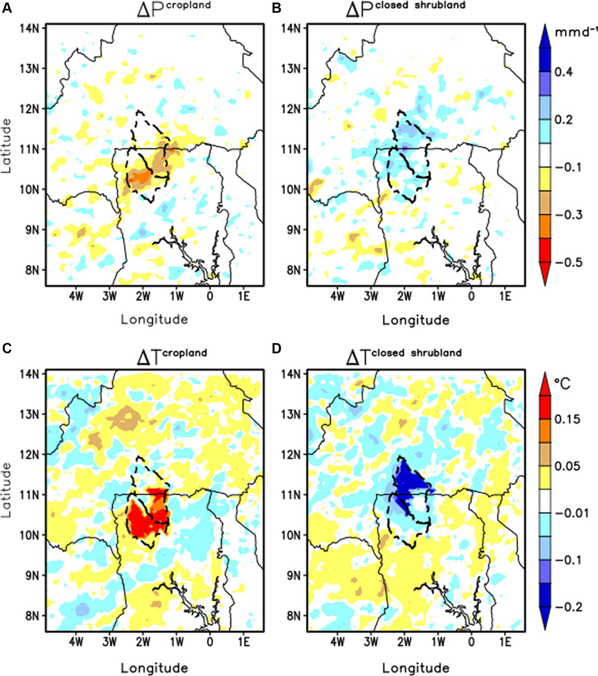
Maps of (A,B) daily precipitation change (in mm/day) and (C,D) daily mean temperature change in (°C) between WRF-Hydro reference experiment and the (A,C) croplands (B,D) closed shrubland. Mean bias values are computed as the difference between the scenario experiments and the reference experiment, averaged over 7 years from 1st January, 2010 to 31st December, 2016. The color scale of the daily precipitation change maps (A,B) is the same as shown beside Figure (B), and the color scale of the daily mean temperature change maps (C,D) is also the same as shown beside Figure (D).
Figure 10

Maps of (A,D) daily mean evaporation change Esoil (in mm/day), (B,F) daily mean plant evapotranspiration change Eplant (in mm/day), (C,G) daily mean daily surface runoff Rsurface change (in mm/day), and (D,H) daily mean underground runoff change Rground (in mm/day), between each scenario experiment: (A–D) cropland, (E–H) closed shrubland, and the WRF-Hydro reference experiment. (A,D) Evaporation from below the soil plus evaporation outside the canopy gives the total soil evaporation. (B,F) Plant transpiration plus water evaporated from canopy interception gives the plant evapotranspiration. The difference between the mean value of each scenario experiment and the reference WRF-Hydro experiment from 1st January, 2010 to 31st December, 2016 yields the mean differential values. The color scale is the same for all water flux maps indicated on the right side of figure extending the width of maps (E–H).
Figure 11

Time series of spatially aggregated monthly climatology of water flow change components of the terrestrial water budget over the SKB area, namely the precipitation change ΔP (in m3/s), the surface runoff change ΔRsurface (in m3/s), the total evapotranspiration change ΔE (in m3/s), the differential change in soil water storage ΔStorageChange (in m3/s), and the underground runoff change ΔRground (in m3/s), between the reference experiment and the (A) closed shrubland, (B) cropland. Monthly climatological change values are computed as the difference between the monthly climatological value of the scenario experiments and the monthly climatological value of the reference experiment from 1st January 2010 to 31st December 2016. (A) provides the legend.
Table 4
| Land cover | Closed shrubland | Cropland | ||
|---|---|---|---|---|
| Area (km2) | Percentage share (%) | Area (km2) | Percentage share (%) | |
| Broadleaf forest | 4,494 | 20.5 | 49,932 | 20.5 |
| Closed shrubland | 15,743 | 71.7 | - | - |
| Wetland | 0.45 | 0.00 | 0.45 | - |
| Cropland | - | - | 15,744 | 71.7 |
| Grassland | 1725 | 7.9 | 1725 | 7.9 |
| Water | 2 | 0.01 | 2 | 0.01 |
Total land cover in km2 and % of each land cover category for each land cover change numerical experiment over the Sissili-Kulpawn Basin (SKB).
3 Results and discussion
3.1 Effects of numerical land cover changes experiment on biophysical parameters
The different land cover change experiments result in different mean albedo and LAI values compared to the reference WRF-Hydro simulation as seen in Figures 3A,D. The WRF-Hydro simulated mean albedo values for cropland, and closed shrubland scenarios over the SKB are 0.25, and 0.17 respectively, compared to a mean reference value of 0.20. This indicates the cropland scenario results in an increase in mean albedo over the SKB by +0.05, while the closed shrubland scenario results in a decrease in the mean albedo over the basin by −0.03, compared to the reference scenario (Figure 3A). The fact that the basin average albedo value for the cropland scenario is higher than that of the closed shrubland scenario is consistent with literature as replacing closed shrubland with cropland is a deforestation scenario that leads to an increase in albedo. Croplands have higher albedo values (0.18–0.25) than closed shrublands (0.16–0.18) which is depicted by our results. The LAI and albedo value changes are in phase opposition, with the LAI increasing (decreasing) as the albedo decreases (increases). The LAI for the cropland, and closed shrubland experiments over the SKB are 1.55 m2m−2, and 2.03 m2m−2, respectively, the reference value being 1.83 m2m−2. The change of the LAI under the cropland, and closed shrubland are, respectively, −0.28 m2m−2, and 0.20 m2m−2, indicating a reduction in LAI for the cropland scenario and an increase in LAI for the closed shrubland scenario compared to the reference scenario (Figure 3D). From the analysis of the albedo and LAI, our model represents well these two biophysical properties of land-atmosphere interactions necessary for simulating the effects of land cover changes on the energy and water budgets.
3.2 Validation of uncalibrated WRF-Hydro simulated rainfall and streamflow
The results of the skill metrics for simulated precipitation and discharge are shown in Figures 4A,B, respectively. The default setup values are indicated in grey and are lower than the corresponding calibrated setup values. For precipitation, the R2, NSE, KGE, and PBIAS for Kulpawn Basin are 0.56, 0.31, 0.64, and − 2.8%, respectively. For daily discharge, these performance values are 0.53, −0.34, 0.2, and − 52.4%, respectively. Thus, the default uncalibrated setup yields relatively weak discharge metrics compared to precipitation, emphasizing the need for calibrating the surface hydrology component. This is evident in the unrealistically high peaks in the simulated discharge in grey (see Figure 4B).
3.3 Validation of calibrated WRF-Hydro simulated rainfall, temperature, and discharge
Figure 5 shows the validation of the calibrated WRF-Hydro simulated rainfall and temperature with IMERG and CHIRTS observational products. The WRF-Hydro simulated mean temperature and precipitation over the SKB are 27.3°C and 2.7 mm day−1, compared to 29.2°C and 2.6 mm day−1 from CHIRTS and IMERG observational products, respectively. The bias is thus −1.7°C and 3.5% showing an underestimation of temperature and overestimation of precipitation. The calibrated WRF-Hydro simulated rainfall shows biases compared to the observational dataset (IMERG) within the range of −25 to +25% (Figure 5C) with underestimations mainly in the northern parts of the inner domain within the upper parts of Sissili in Burkina Faso. Lower overestimations within −10 to 10% are mainly constrained to the southern parts covering the entire KB and the lower parts of SB. The relatively lower bias of simulated rainfall in the KB could explain the relatively good performance in the discharge evaluation metrics at Yagaba on the Kulpawn River, with the R2, NSE, KGE, and PBIAS of 0.53, 0.47, 0.69, and − 15%, respectively. Yet, the moderate performance in simulated discharge could be attributed to the quality of the simulated precipitation (see Figure 5C), a well-known limitation of the coupled atmospheric-hydrological modeling approach (Senatore et al., 2015). The moderate NSE metrics fall within the range of published precipitation and discharge performance across the globe: 0.46 for (Arnault et al., 2016a), 0.27 for (Kerandi et al., 2018), −1.89–0.61 for (Rummler et al., 2019), 0.27 for (Li et al., 2020), 0.30 for (Arnault et al., 2023). More importantly, the calibrated setup improves both rainfall and discharge over the SKB compared to the default setup (see metrics in Figures 4A,B). Consequently, the rainfall-discharge results obtained over the calibration period are considered realistic and the WRF-Hydro with two-way river-land flow option is adopted to investigate the climate response to land cover changes in this work. The biases in precipitation show that the fully coupled WRF-Hydro simulated temperature and precipitation biases are minimal such that the model is skilled in providing climate information on daily timescales. In West Africa, rainfall and temperature are the most basic information provided by national meteorological organizations to the public. With the capabilities of the fully coupled WRF/WRF-Hydro shown in this work, national meteorological agencies can use the WRF model to complement or improve the traditional approach to weather forecasting. That said, the WRF-Hydro simulations are computationally expensive, and strong computational resources and skills are required to run simulations. The employees of the national meteorological agencies must be skilled to simulate, analyze the results, and make reports available to the public as climate information or weather forecasts. The traditional way of forecasting and climate information provision could significantly benefit from the fully coupled WRF/WRF-Hydro.
Figure 5
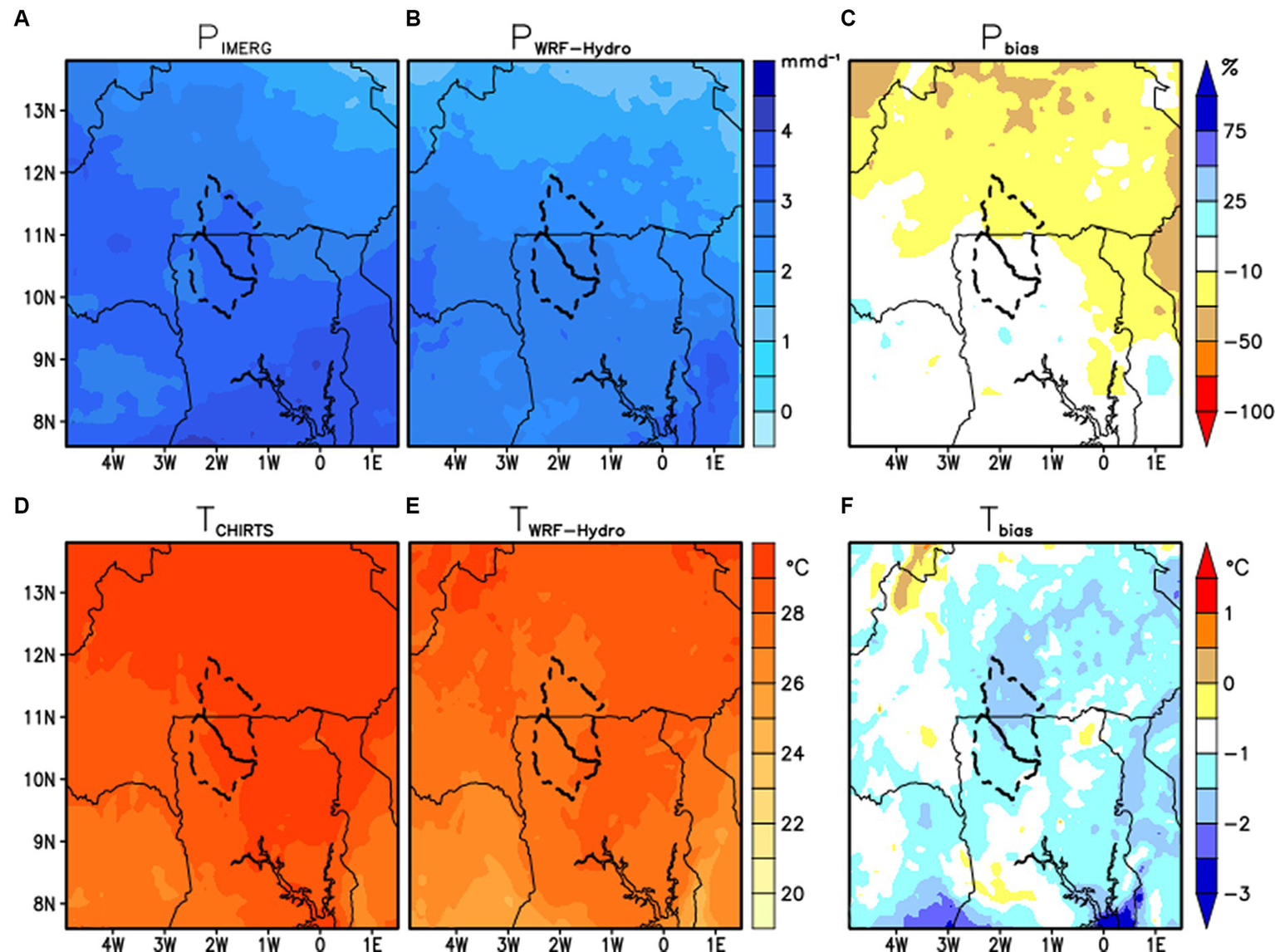
Maps of (A) daily IMERG mean precipitation P (in mm/day), (B) daily WRF-Hydro reference mean precipitation (in mm/day), (C) percentage bias (in %) between WRF-Hydro reference precipitation and IMERG, (D) daily mean CHIRTS temperature T (in °C), (E) daily WRF-Hydro reference mean temperature (in °C), (F) percentage bias (in °C) between CHIRTS temperature and WRF-Hydro reference temperature. Precipitation maps (A,B) share the same color scale shown beside (B), and the temperature maps (D,E) also share the same color scale beside (E). Mean precipitation and temperature values are calculated from 1st January, 2010 to 31st December, 2016.
3.4 Validation of simulated energy fluxes
The percentage bias of the WRF-Hydro simulated Rnet, Hsensible, and Hlatent fluxes in the inner domain ranges between −25 to 10%, −10 to 50%, and − 50 to 10%, respectively, (see Figures 6C,F,I), over the 2013–2016 period. Over the SKB, the average percentage bias of Rnet, Hsensible, and Hlatent is 11, 31% and − 4% indicating an overestimation of Rnet and Hsensible but an underestimation of the Hlatent flux. In terms of numerical values, the mean Rnet averaged over SKB is 135 Wm−2 compared to 121 Wm−2 from the FLUXCOM observation product. The mean simulated Hsensible is 70 Wm−2 compared to 53 Wm−2 from the FLUXCOM observation product. Finally, the mean Hlatent flux is 65 Wm−2 compared to 69 Wm−2 over the 2010–2013 period. The overestimation of Hsensible and underestimation of Hlatent suggests that the modeled land compartment is too dry.
Figure 6

Maps of (A) mean net radiation flux (Rnet) in W/m2 from FLUXCOM observational product, (B) mean net radiation flux Rnet from reference WRF-Hydro simulation, (C) Rnet bias (in %) between observation product FLUXCOM and reference WRF-Hydro simulations, (D) mean net sensible heat flux Hsensible (in W/m2) from observation product FLUXCOM, (E) mean net sensible heat flux Hsensible (in W/m2) from the WRF-Hydro reference simulations (F) sensible heat flux bias (in %) between FLUXCOM observation product and WRF-Hydro reference simulation, (G) mean latent heat flux Hlatent from the observation product FLUXCOM, (H) mean latent heat flux Hlatent from WRF-Hydro reference simulation, (I) latent heat flux bias (in %) between observation product and WRF-Hydro reference simulation. The energy flux maps (A,B,D,E,G,H) have the same color scale shown below figure and extend the widths of maps (G–I). The bias maps (C,F,I) have the same color maps shown at the right side of figure and extends the heights of (C,F,I). Mean flux values are computed for 4 years spanning from 1st January 2010 to 31st December 2013.
3.5 Seasonal climatology evaluation of simulated rainfall, discharge, temperature and energy fluxes over Sissili-Kulpawn Basin
The climatology of WRF-Hydro simulated rainfall over the SKB is close to IMERG observational product, with mostly underestimations, except for a slight overestimation of June–July–August–September (JJAS) rainfall (Figure 7A). Thus, the WRF-Hydro with riverbank overflow option improves the simulated rainfall but is a little wetter than that observed in JJAS over the SKB. The impact of the JJAS simulated rainfall on discharge is resolved by the overbank flow option in the updated WRF-Hydro such that the discharge in JJAS stays very close to the observed discharge (Figure 7B), with only a slight overestimation in September. The WRF-Hydro simulated temperature also underestimates the CHIRTS observational product but stays very close in the April–May–June–July (AMJJ) period (Figure 7C). In terms of Rnet, the WRF-Hydro simulation mimics well the observational product FLUXCOM for January–February–March–April (JFMA) and June–July–August (JJA) with the most overestimations at May–June (MJ) and September–October–November–December (SOND) periods. The simulated Hsensible overestimates the observational product for all months, while the Hlatent underestimates the FLUXCOM data for nearly all months of the year except December (Figure 7D). From the foregoing, the simulated rainfall (P), temperature (T), discharge, Rnet, Hsensible, and Hlatent show that the WRF-Hydro with overbank flow extension as used in this study mimics reasonably the hydroclimatic situation of the SKB and can be considered for providing climate service for the region.
Figure 7

Monthly climatological time series of (A) basin-averaged Precipitation P over SKB in mm/month, (B) average Discharge Q at Yagaba-Wiasi gauges in m3/s, (C) basin-averaged Temperature over SKB in °C, (D) basin-averaged Sensible (Hsensible), net radiation (Rnet), and latent heat fluxes (Hlatent) over SKB in W/m2, as derived from (A) the IMERG observations, (B) gauge measurement, (C) the CHIRTS observations, (D) the FLUXCOM observations and the reference WRF-Hydro experiment over the inner domain. Climatological values are calculated over (A–C) 7 years starting from 1st January, 2010 to 31st December, 2016 (D) 4 years starting from 1st January, 2010 to 31st December, 2013, when corresponding observed data is available.
3.6 Impact of land cover change on energy fluxes
The average changes in the Rnet, Hsensible, Hlatent over the SKB for the cropland scenario are obtained from Figures 8A–C and evaluated as −11 Wm−2, −9 Wm−2, and − 2 Wm−2, respectively. For the closed shrubland, the changes in Rnet, Hsensible, and Hlatent over the SKB is evaluated from Figures 8D–F as +7 Wm−2, +5 Wm−2, and + 2 Wm−2, respectively. From the results above, on the one hand, the cropland scenario decreases the Rnet, Hsensible, and Hlatent fluxes compared to the closed shrubland scenario which results in a net increased energy flux. As mentioned previously, the decrease in Rnet, Hsensible, and Hlatent fluxes for the cropland is related to the increase in the albedo (see Figure 3B) and a decrease in LAI (see Figure 3E) which reduces Rnet, Hsensible, and Hlatent fluxes (see Figures 8A–C). In contrast, the decreased albedo (see Figure 3C) and increased LAI (see Figure 3F) for the closed shrubland scenario increase absorption of incoming radiation but decreases outgoing radiation to space, thus resulting in surplus energy near the surface which increases Rnet, Hsensible, and Hlatent fluxes (see Figures 8D–F).
3.7 Impacts of land cover change on temperature and precipitation
The change in precipitation and temperature averaged over SKB between the cropland and the reference scenario estimated is −0.1 mm day−1 and + 0.1°C respectively. For the closed shrubland scenario, the change in precipitation and temperature over the SKB is +0.1 mm day−1 and -0.1°C. Accordingly, there is an increase in temperature and a decrease in precipitation for the cropland but a decrease in temperature and an increase in precipitation for the closed shrubland scenario. For the closed shrubland scenario, the surface temperature increase through enhanced sensible heating is offset by an enhanced evaporative cooling from the soil and plant surface (see Figures 10E,F). Consequently, the temperature for the closed shrubland scenario decreases as can be seen in Figure 9D. The evaporative cooling also enhances atmospheric moisture and consequently increases precipitation for the closed shrubland scenario (see Figure 9B). Conversely, the cropland scenario behaves as a deforestation scenario where there is an increase in albedo but a decrease in LAI. As a result, net radiation (see Figure 8A) and heat fluxes (see Figures 8B,C) are decreased and less energy is available for evaporative cooling through soil and plant evaporation, consequently increasing the temperature (Figure 9C). The reduced evaporation affects the amount of moisture in the atmosphere to precipitate back as rainfall, hence the observed reduction of rainfall for the cropland scenario (see Figure 6A). It is noted that non-radiative forcing is the dominant factor affecting temperature in the tropics (Zhang et al., 2022), such that afforestation usually results in a decrease in temperature (Betts, 2000; Li et al., 2015). Lawrence and Vandecar (2015) using satellite towers, and ground-based observations have shown that tropical deforestation results in warmer, drier conditions at the local scale. The closed shrubland scenario, which decreases albedo and increases LAI similar to an afforestation scenario, tends to decrease temperature and increase precipitation, which confirms the strong correlation between land surface and climate variables discussed by Hardwick et al. (2015). Conversely, the cropland scenario which tends to increase albedo and decrease LAI is consistent with a deforestation scenario, resulting in an increase in temperature and a decrease in the precipitation. From the foregoing, we conclude that our numerical experiment can provide a sound prediction of the impacts of afforestation and deforestation scenarios on regional temperature and precipitation. The results show that afforestation or deforestation could modulate the local climate by decreasing or increasing temperature and rainfall. The synthetic numerical experiments conducted in this work are extreme cases of deforestation and afforestation with positive and negative impacts (see Tables 3, 4 for the percentage area afforested/deforested). In that sense, the community can benefit from a controlled afforestation scenario that prevents the adverse effects of flooding associated with the extreme afforestation scenario. Conversely, farmers or the SKB project could benefit from controlled cropland expansion that does not significantly affect rainfall. Land managers could benefit from the threshold values of deforestation and afforestation used in this work to guide land management in the basin. This practice will ensure the climate-land-water-energy-food balance in the basin with no adverse effects.
3.8 Impact of land cover change on water fluxes
For the cropland scenario, the ΔEsoil, ΔEplant, ΔRsurface, ΔRground over the SKB are estimated from Figures 10A–D as −0.05 mm day−1, −0.01 mm day−1, −0.03 mm day−1, and − 0.0004 mm day−1, respectively. In terms of the closed shrubland scenario, ΔEsoil, ΔEplant, ΔRsurface, ΔRground are estimated as +0.03 mm day−1, +0.03 mm day−1, +0.03 mm day−1, and + 0.00006 mm day−1 (see Figures 10E,F). We recall a slightly higher net positive change in Rnet, Hsensible, and Hlatent for the closed shrubland scenario compared to the cropland (see Figure 8). These surface energy flux changes enhance soil evaporation and plant transpiration in the closed shrubland scenario (see Figures 10E,F) compared to the cropland scenario (see Figures 10A,B). The enhancement of the soil evaporation and plant transpiration increases atmospheric moisture to precipitate back as rainfall leading to higher surface runoff in the closed shrubland scenario (see Figure 10G). Conversely, in the cropland scenario, the decrease in soil evaporation and plant transpiration reduces moisture in the atmosphere to precipitate back as rainfall consequently reducing the surface runoff (see Figure 10C). In both scenarios, however, there is an insignificant change in underground runoff over the SKB. The climatological water flow change of the closed shrubland afforestation scenario (see Figure 11A) shows an average increase in precipitation of +6%, evapotranspiration of +3%, surface runoff of +27%, and underground runoff of +16% (see Table 5). In the cropland scenario, the simulated annual water flow changes of precipitation, evapotranspiration, surface runoff, and underground runoff over SKB all decreased by −5, −3%, and − 9%, respectively, (Table 5) relative to the reference scenario. In general, our numerical land cover change experiment realistically mimics the regional water cycle response to changes in biophysical properties.
Table 5
| Variable | Closed shrubland | Cropland | ||
|---|---|---|---|---|
| Annual depth of water change (mm/year) | Relative water flow change (%) | Annual depth of water change (mm/year) | Relative water flow change (%) | |
| 44.5 | 5.6 | −49.0 | −4.8 | |
| 22.2 | 3.1 | −24.2 | −3.0 | |
| 10.7 | 27.1 | −12.1 | −2.5 | |
| −0.02 | 15.9 | −0.13 | −9.3 | |
Differential changes in water flow terms over the Sissili-Kulpawn River Basin.
Annual simulated changes in water flow in mm/year, and annual percentage changes in water flow in % relative to the annual reference values due to afforestation (deforestation) scenario for precipitation, surface runoff , total evapotranspiration , underground runoff , from 1st January 2010 to 31st December 2016 over the SKB. In this table, a differential value is defined as the scenario experiment (afforestation or deforestation) value minus the reference WRF-Hydro simulated value.
4 Summary and conclusion
The regional climate response to introducing the European Space Agency (ESA)'s annual 300 m land cover data into the fully-coupled WRF-Hydro to simulate its effects on the regional water and energy cycle was investigated for the Sissili-Kulpawn Basin in tropical West Africa. The setup consists of an outer domain at 50 km resolution, an inner domain at 10 km resolution, and a sub-domain at 1 km resolution coupled with the inner domain for water routing computations. The primary advantage of this setup lies in its coarse resolution (less computationally expensive), yet its ability to mimics well the regional climate. The implementation of a two-way water-land river extension of the default WRF-Hydro further allows for reducing unrealistically high discharges associated with flat or complex terrain which is missing in the default WRF-Hydro. The experimental design and settings explore benefits spanning from a global perspective through regional to local scales. From a global perspective, this paper evaluates the suitability of ESA global annual 300 m land cover data as an alternative land cover data for the WRF-Hydro modeling system. On a regional scale, this research evaluates the WRF-Hydro (with ESA LC) reproducibility of the regional climate as well as the water and energy cycles as a tool for providing climate services for the West African region. On a more local scale, this work assesses how huge (72%) afforestation and deforestation could impact water availability in the Sissili-Kulpawn Basin which is already vulnerable to annual flooding events. Therefore, the default MODIS land cover data in the WRF-Hydro was replaced by the relatively high-resolution ESA LC data to generate a control experiment and assess its reproducibility of regional climate using observational data products. Two synthetic numerical land cover change experiments (a) afforestation by closed shrubland expansion, and (b) deforestation by cropland expansion, were designed, and the difference between the control experiment and the scenarios were used to determine the regional impacts of the afforestation and deforestation scenarios. The basin-averaged changes in water fluxes were used to determine the impact of water yield and potential impact on already existing flood and drought risks. In general, the control experiment mimics well temperature, water, and energy fluxes indicating the fully-coupled WRF-Hydro with ESA LC is suitable for supporting climate services for the region. The closed shrubland afforestation and cropland deforestation scenarios increased and decreased water yield, respectively, consistent with the well-known effects of afforestation and deforestation in tropical regions. As such, the fully-coupled WRF-Hydro with ESA LC can also be considered suitable for modeling the effects of land use and land cover change on regional climate. On the one hand, the cropland scenario reveals that deforestation of an additional 44% of closed shrubland for food production could result in a decrease in annual water yield, which can provide suitable conditions for drought. This threshold should therefore be considered by initiatives like the Sissili-Kulpawn Basin project which aims to help smallholder farmers expand agriculture through irrigation. On the other hand, afforesting an additional 28% of closed shrubland could increase the annual water yield and increase the already existing annual flooding risk in the SKB. To this end, moderate afforestation is recommended for the SKB to increase the water yield but limit the area of cropland loss due to reforestation, and also to minimize the enhanced flood risk conditions. The role of policymakers in this regard is to invest in the computational resources, more in situ measurements, and training of skilled personnel needed to run WRF/WRF-Hydro and make the climate information and forecast available on time. A practical approach is to start with the national meteorological agencies of respective countries by equipping them with a high-performance computing infrastructure needed to run country-wide simulations, preferably at high resolution. More importantly, personnel within the same organizations can be equipped with skills to use and maintain these high-performance computing systems. Currently, WRF/WRF-Hydro is not fully operational because of the above-mentioned challenges. The national metrological agencies rely on forecasts from ECMWF (European Centre for Medium-Range Weather Forecasts) for operational forecasting. WRF runs serve hindcasting purposes where the WRF outputs are compared with observations. So, the West African region could benefit from the capabilities of the WRF/WRF-Hydro model if policymakers can put these structures in place.
Statements
Data availability statement
The original contributions presented in the study are included in the article, further inquiries can be directed to the corresponding author.
Author contributions
EM: Conceptualization, Data curation, Formal analysis, Investigation, Methodology, Software, Validation, Visualization, Writing – original draft, Writing – review & editing. JA: Conceptualization, Data curation, Formal analysis, Investigation, Methodology, Software, Supervision, Validation, Writing – review & editing. MI: Data curation, Supervision, Writing – review & editing. SM: Data curation, Supervision, Writing – review & editing. TA: Data curation, Supervision, Writing – review & editing, Methodology. PL: Data curation, Writing – review & editing. MD: Data curation, Writing – review & editing. HK: Funding acquisition, Resources, Supervision, Writing – review & editing.
Funding
The author(s) declare that financial support was received for the research, authorship, and/or publication of this article. This research was supported by the Federal Ministry of Education and Research of Germany (BMBF) through the West African Science Service Center on Climate Change and Adapted Land Use (WASCAL), by the German Science Foundation (DFG) through the Large-Scale and High-Resolution Mapping of Soil Moisture on Field and Catchment Scales Boosted by Cosmic-Ray Neutrons (COSMIC-SENSE, FOR 2694, grant KU 2090/12-2) and Climate Change and Health in sub-Saharan Africa (FOR 2936, grant KU 2090-14/2).
Acknowledgments
The simulations were conducted at the linux cluster of KIT/IMK-IFU in Garmisch-Partenkirchen, designed and maintained by Benjamin Fersch and Frank Neidl. The Sissili-Kulpawn river discharge data was provided by the Volta Basin Authority (VBA) at Ouagadougou, Burkina Faso.
Conflict of interest
The authors declare that the research was conducted in the absence of any commercial or financial relationships that could be construed as a potential conflict of interest.
The author(s) declared that they were an editorial board member of Frontiers, at the time of submission. This had no impact on the peer review process and the final decision.
Publisher’s note
All claims expressed in this article are solely those of the authors and do not necessarily represent those of their affiliated organizations, or those of the publisher, the editors and the reviewers. Any product that may be evaluated in this article, or claim that may be made by its manufacturer, is not guaranteed or endorsed by the publisher.
References
1
Achugbu I. C. Laux P. Olufayo A. A. Balogun I. A. Dudhia J. Arnault J. et al . (2022a). The impacts of land use and land cover change on biophysical processes in West Africa using a regional climate model experimental approach. Int. J. Climatol.43, 1731–1755. doi: 10.1002/joc.7943
2
Achugbu I. C. Olufayo A. A. Balogun I. A. Adefisan E. A. Dudhia J. Naabil E. (2021). Modeling the spatiotemporal response of dew point temperature, air temperature and rainfall to land use land cover change over West Africa. Model. Earth Syst. Environ.8, 173–198. doi: 10.1007/s40808-021-01094-8
3
Achugbu I. C. Olufayo A. A. Balogun I. A. Dudhia J. McAllister M. Adefisan E. A. et al . (2022b). Potential effects of land use land cover change on streamflow over the Sokoto Rima River basin. Heliyon8:e09779. doi: 10.1016/j.heliyon.2022.e09779
4
Arnault J. Fersch B. Rummler T. Zhang Z. Quenum G. M. Wei J. et al . (2021). Lateral terrestrial water flow contribution to summer precipitation at continental scale–a comparison between Europe and West Africa with WRF-hydro-tag ensembles. Hydrol. Process.35:e14183. doi: 10.1002/hyp.14183
5
Arnault J. Knoche R. Wei J. Kunstmann H. (2016a). Evaporation tagging and atmospheric water budget analysis with WRF: a regional precipitation recycling study for West Africa. Water Resour. Res.52, 1544–1567. doi: 10.1002/2015WR017704
6
Arnault J. Mwanthi A. M. Portele T. Li L. Rummler T. Fersch B. et al . (2023). Regional water cycle sensitivity to afforestation: synthetic numerical experiments for tropical Africa. Front. Climate5:1233536. doi: 10.3389/fclim.2023.1233536
7
Arnault J. Wagner S. Rummler T. Fersch B. Bliefernicht J. Andresen S. et al . (2016b). Role of runoff–infiltration partitioning and resolved overland flow on land–atmosphere feedbacks: a case study with the WRF-hydro coupled modeling system for West Africa. J. Hydrometeorol.17, 1489–1516. doi: 10.1175/JHM-D-15-0089.1
8
Bagley J. E. Desai A. R. Harding K. J. Snyder P. K. Foley J. A. (2014). Drought and deforestation: has land cover change influenced recent precipitation extremes in the Amazon?J. Clim.27, 345–361. doi: 10.1175/JCLI-D-12-00369.1
9
Betts R. A. (2000). Offset of the potential carbon sink from boreal forestation by decreases in surface albedo. Nature408, 187–190. doi: 10.1038/35041545
10
Bliefernicht J. Berger S. Salack S. Guug S. Hingerl L. Heinzeller D. et al . (2018). The WASCAL hydrometeorological observatory in the Sudan savanna of Burkina Faso and Ghana. Vadose Zone J.17, 1–20. doi: 10.2136/vzj2018.03.0065
11
Bonan G. B. (2008). Forests and climate change: forcings, feedbacks, and the climate benefits of forests. Science320, 1444–1449. doi: 10.1126/science.1155121
12
Burakowski E. A. Ollinger S. V. Bonan G. B. Wake C. P. Dibb J. E. Hollinger D. Y. (2016). Evaluating the climate effects of reforestation in New England using a weather research and forecasting (WRF) model multiphysics ensemble. J. Clim.29, 5141–5156. doi: 10.1175/JCLI-D-15-0286.1
13
Cao Q. Wu J. Yu D. Wang W. (2019). The biophysical effects of the vegetation restoration program on regional climate metrics in the loess plateau, China. Agric. For. Meteorol.268, 169–180. doi: 10.1016/j.agrformet.2019.01.022
14
Cerbelaud A. Lefèvre J. Genthon P. Menkes C. (2022). Assessment of the WRF-hydro uncoupled hydro-meteorological model on flashy watersheds of the Grande Terre tropical island of New Caledonia (south-West Pacific). J. Hydrol.40:101003. doi: 10.1016/j.ejrh.2022.101003
15
Chapin F. S. Sturm M. Serreze M. C. McFadden J. P. Key J. R. Lloyd A. H. et al . (2005). Role of land-surface changes in Arctic summer warming. Science310, 657–660. doi: 10.1126/science.1117368
16
Chen C. Ge J. Guo W. Cao Y. Liu Y. Luo X. et al . (2022). The biophysical impacts of idealized afforestation on surface temperature in China: local and nonlocal effects. J. Clim.35, 7833–7852. doi: 10.1175/JCLI-D-22-0144.1
17
Chen S. Tian L. Zhang B. Zhang G. Zhang F. Yang K. et al . (2023). Quantifying the impact of large-scale afforestation on the atmospheric water cycle during rainy season over the Chinese loess plateau. J. Hydrol.619:129326. doi: 10.1016/j.jhydrol.2023.129326
18
de Noblet-Ducoudré N. Boisier J. P. Pitman A. Bonan G. B. Brovkin V. Cruz F. et al . (2012). Determining robust impacts of land-use-induced land cover changes on surface climate over North America and Eurasia: results from the first set of LUCID experiments. J. Clim.25, 3261–3281. doi: 10.1175/JCLI-D-11-00338.1
19
Defourny P. Bontemps S. Lamarche C. Brockmann C. Boettcher M. et al . (2017) Land cover CCI: product user guide version 2.0. Available at: http://maps.elie.ucl.ac.be/CCI/viewer (Accessed March 3, 2023).
20
Deng X. Güneralp B. Zhan J. Su H. (2014). Land use impacts on climate. Cham: Springer.
21
Deng X. Liu J. Ma E. Jiang L. Yu R. Jiang Q. O. et al . (2015). “Impact assessments on water and heat fluxes of terrestrial ecosystem due to land use change,” in Impacts of Land-use Change on Ecosystem Services, Eds. J. Zhan, Springer Geography. Berlin, Heidelberg: Springer.
22
Dickinson R. E. Henderson-Sellers A. (1988). Modelling tropical deforestation: a study of GCM land-surface parametrizations. Q. J. R. Meteorol. Soc.114, 439–462. doi: 10.1002/qj.49711448009
23
Dixit A. Sahany S. Rajagopalan B. Choubey S. (2022). Role of changing land use and land cover (LULC) on the 2018 megafloods over Kerala, India. Clim. Res.89, 1–14. doi: 10.3354/cr01701
24
Dudhia J. (1989). Numerical study of convection observed during the winter monsoon experiment using a mesoscale two-dimensional model. J. Atmos. Sci.46, 3077–3107. doi: 10.1175/1520-0469(1989)046<3077:NSOCOD>2.0.CO;2
25
Eghdami M. Barros A. P. (2020). Deforestation impacts on orographic precipitation in the tropical Andes. Front. Environ. Sci.8:580159. doi: 10.3389/fenvs.2020
26
Eiras-Barca J. Dominguez F. Yang Z. Chug D. Nieto R. Gimeno L. et al . (2020). Changes in south American hydroclimate under projected Amazonian deforestation. Ann. N. Y. Acad. Sci.1472, 104–122. doi: 10.1111/nyas.14364
27
Feddema J. J. Oleson K. W. Bonan G. B. Mearns L. O. Buja L. E. Meehl G. A. et al . (2005). The importance of land-cover change in simulating future climates. Science310, 1674–1678. doi: 10.1126/science.1118160
28
Fersch B. Kunstmann H. (2014). Atmospheric and terrestrial water budgets: sensitivity and performance of configurations and global driving data for long term continental scale WRF simulations. Clim. Dyn.42, 2367–2396. Available at: Doi:10. 1007/s00382-013-1915-5. doi: 10.1007/s00382-013-1915-5
29
Foley J. A. DeFries R. Asner G. P. Barford C. Bonan G. Carpenter S. R. et al . (2005). Global consequences of land use. Science309, 570–574. doi: 10.1126/science.1111772
30
Garcia M. Özdogan M. Townsend P. A. (2014). Impacts of forest harvest on cold season land surface conditions and land-atmosphere interactions in northern Great Lakes states. J. Adv. Model. Earth Syst.6, 923–937. doi: 10.1002/2014MS000317
31
Gochis D. J. Barlage M. Cabell R. Casali M. Dugger A. FitzGerald K. et al . (2021). The WRF-hydro R modeling system technical description, (version 5.2.0). NCAR technical note. Available at: https://ral.ucar.edu/sites/default/files/public/projects/wrf-hydro/technical-description-user-guide/wrf-hydrov5.2technicaldescription.Pdf
32
Graf M. Arnault J. Fersch B. Kunstmann H. (2021). Is the soil moisture precipitation feedback enhanced by heterogeneity and dry soils? A comparative study. Hydrol. Process.35:e14332. doi: 10.1002/hyp.14332
33
Grell G. A. Freitas S. R. (2014). A scale and aerosol aware stochastic convective parameterization for weather and air quality modeling. Atmos. Chem. Phys.14, 5233–5250. doi: 10.5194/acp-14-5233-2014
34
Gross E. Pennink C. (2018) Impact Evaluation of the Sustainable Water Fund (FDW) Integrated Water Management and Knowledge Transfer in Sisili Kulpawn Basin (FDW/12/GH/02) in the Northern Region of Ghana Final report December 2018.
35
Gupta H. V. Kling H. Yilmaz K. K. Martinez G. F. (2009). Decomposition of the mean squared error and NSE performance criteria: implications for improving hydrological modelling. J. Hydrol.377, 80–91. doi: 10.1016/j.jhydrol.2009.08.003
36
Hardwick S. R. Toumi R. Pfeifer M. Turner E. C. Nilus R. Ewers R. M. (2015). The relationship between leaf area index and microclimate in tropical forest and oil palm plantation: Forest disturbance drives changes in microclimate. Agric. For. Meteorol.201, 187–195. doi: 10.1016/j.agrformet.2014.11.010
37
Hersbach H. Bell B. Berrisford P. Hirahara S. Horányi A. Muñoz-Sabater J. et al . (2020). The ERA5 global reanalysis. Q. J. R. Meteorol. Soc.146, 1999–2049. doi: 10.1002/qj.3803
38
Hong S. Y. Lim J. O. J. (2006). The WRF single-moment 6-class microphysics scheme (WSM6). Asia Pac. J. Atmos. Sci.42, 129–151.
39
Huffman G. Bolvin D. Braithwaite D. Hsu K. Joyce R. Xie P. (2014). Integrated multi-satellitE retrievals for GPM (IMERG), version 4.4. NASA’s precipitation processing center. Available at: https://disc.gsfc.nasa.gov/datasets/GPM_3IMERGDF_06/summary?Keywords=IMERGfinal (Accessed February 12, 2023).
40
Jach L. Warrach-Sagi K. Ingwersen J. Kaas E. Wulfmeyer V. (2020). Land cover impacts on land-atmosphere coupling strength in climate simulations with WRF over Europe. J. Geophys. Res. Atmos.125:e2019JD031989. doi: 10.1029/2019JD031989
41
Jung M. Koirala S. Weber U. Ichii K. Gans F. Camps-Valls G. et al . (2019). The FLUXCOM ensemble of global land-atmosphere energy fluxes. Sci. Data6:74. doi: 10.1038/s41597-019-0076-8
42
Kerandi N. Arnault J. Laux P. Wagner S. Kitheka J. Kunstmann H. (2018). Joint atmospheric-terrestrial water balances for East Africa: a WRF-hydro case study for the upper Tana River basin. Theor. Appl. Climatol.131, 1337–1355. doi: 10.1007/s00704-017-2050-8
43
Kerandi N. M. Laux P. Arnault J. Kunstmann H. (2017). Performance of the WRF model to simulate the seasonal and interannual variability of hydrometeorological variables in East Africa: a case study for the Tana River basin in Kenya. Theor. Appl. Climatol.130, 401–418. doi: 10.1007/s00704-016-1890-y
44
Kishtawal C. M. Niyogi D. Tewari M. Pielke R. A. Sr. Shepherd J. M. (2010). Urbanization signature in the observed heavy rainfall climatology over India. Int. J. Climatol.30, 1908–1916. doi: 10.1002/joc.2044
45
Laux P. Dieng D. Portele T. C. Wei J. Shang S. Zhang Z. et al . (2021). A high-resolution regional climate model physics ensemble for northern sub-Saharan Africa. Front. Earth Sci.9:700249. doi: 10.3389/feart.2021.700249
46
Laux P. Nguyen P. N. B. Cullmann J. Kunstmann H. (2017). “Impacts of land-use/land-cover change and climate change on the regional climate in the central vietnam” in Land use and climate change interactions in Central Vietnam Eds. A. Nauditt and L. Ribbe, Singapore: Springer.
47
Lawrence D. Vandecar K. (2015). Effects of tropical deforestation on climate and agriculture. Nat. Clim. Chang.5, 27–36. doi: 10.1038/nclimate2430
48
Lee J. Seo J. M. Baik J. J. Park S. B. Han B. S. (2020). A numerical study of windstorms in the Lee of the Taebaek Mountains, South Korea: characteristics and generation mechanisms. Atmos11:431. doi: 10.3390/atmos11040431
49
Lehner B. Verdin K. Jarvis A. (2008). New global hydrography derived from spaceborne elevation data. EOS Trans. Am. Geophys. Union89, 93–94. doi: 10.1029/2008EO100001
50
Li Z. Deng X. Shi Q. Ke X. Liu Y. (2013). Modeling the impacts of boreal deforestation on the near-surface temperature in European Russia. Adv. Meteorol.2013, 1–9. doi: 10.1155/2013/486962
51
Li L. Gochis D. J. Sobolowski S. Mesquita M. D. (2017). Evaluating the present annual water budget of a Himalayan headwater river basin using a high-resolution atmosphere-hydrology model. J. Geophys. Res. Atmos.122, 4786–4807. doi: 10.1002/2016JD026279
52
Li L. Pontoppidan M. Sobolowski S. Senatore A. (2020). The impact of initial conditions on convection-permitting simulations of a flood event over complex mountainous terrain. Hydrol. Earth Syst. Sci.24, 771–791. doi: 10.5194/hess-24-771-2020
53
Li Y. Zhao M. Motesharrei S. Mu Q. Kalnay E. Li S. (2015). Local cooling and warming effects of forests based on satellite observations. Nat. Commun.6:6603. doi: 10.1038/ncomms7603
54
Liu Y. Ge J. Guo W. Cao Y. Chen C. Luo X. et al . (2023). Revisiting biophysical impacts of greening on precipitation over the loess plateau of China using WRF with water vapor tracers. Geophys. Res. Lett.50:e2023GL102809. doi: 10.1029/2023GL102809
55
Ma E. Deng X. Zhang Q. Liu A. (2014). Spatial variation of surface energy fluxes due to land use changes across China. Energies7, 2194–2206. doi: 10.3390/en7042194
56
Ma E. Liu A. Li X. Wu F. Zhan J. (2013). Impacts of vegetation change on the regional surface climate: a scenario-based analysis of afforestation in Jiangxi Province, China. Adv. Meteorol.2013, 1–8. doi: 10.1155/2013/796163
57
Mekonnen K. Velpuri N. M. Leh M. Akpoti K. Owusu A. Tinonetsana P. et al . (2023). Accuracy of satellite and reanalysis rainfall estimates over Africa: a multi-scale assessment of eight products for continental applications. J. Hydrol.49:101514. doi: 10.1016/j.ejrh.2023.101514
58
Mercer A. Dyer J. (2021). Identification of dominant warm-season latent heat flux patterns in the lower Mississippi River Alluvial Valley. Proc. Comput. Sci.185, 1–8. doi: 10.1016/j.procs.2021.05.001
59
Milovac J. Branch O. L. Bauer H. S. Schwitalla T. Warrach-Sagi K. Wulfmeyer V. (2016). High-resolution WRF model simulations of critical land surface-atmosphere interactions within arid and temperate climates (WRFCLIM).In High Performance Computing in Science and Engineering´ 15: Transactions of the High Performance Computing Center, Stuttgart (HLRS) 2015, 607–622. Springer International Publishing.
60
Mlawer E. J. Taubman S. J. Brown P. D. Iacono M. J. Clough S. A. (1997). Radiative transfer for inhomogeneous atmospheres: RRTM, a validated correlated-k model for the longwave. J. Geophys. Res. Atmos.102, 16663–16682. doi: 10.1029/97JD00237
61
Mooney P. A. Lee H. Sobolowski S. (2021). Impact of quasi-idealized future land cover scenarios at high latitudes in complex terrain. Earths Future9:e2020EF001838. doi: 10.1029/2020EF001838
62
Mortey E. M. Annor T. Arnault J. Inoussa M. M. Madougou S. Kunstmann H. et al . (2023). Interactions between climate and land cover change over West Africa. Land12:355. doi: 10.3390/land12020355
63
Nakanishi M. Niino H. (2004). An improved Mellor–Yamada level-3 model with condensation physics: its design and verification. Bound. Layer Meteorol.112, 1–31. doi: 10.1023/B:BOUN.0000020164.04146.98
64
Nash J. E. Sutcliffe J. V. (1970). River flow forecasting through conceptual models part I—A discussion of principles. J. Hydrol.10, 282–290. doi: 10.1016/0022-1694(70)90255-6
65
Niu G. Y. Yang Z. L. Mitchell K. E. Chen F. Ek M. B. Barlage M. et al . (2011). The community Noah land surface model with multiparameterization options (Noah-MP): 1. Model description and evaluation with local-scale measurements. J. Geophys. Res. Atmos.116:D12109. doi: 10.1029/2010JD015139
66
Niyogi D. Kishtawal C. Tripathi S. Govindaraju R. S. (2010). Observational evidence that agricultural intensification and land use change may be reducing the Indian summer monsoon rainfall. Water Resour. Res.46:7082. doi: 10.1029/2008WR007082
67
Odoulami R. C. Abiodun B. J. Ajayi A. E. (2019). Modelling the potential impacts of afforestation on extreme precipitation over West Africa. Clim. Dyn.52, 2185–2198. doi: 10.1007/s00382-018-4248-6
68
Parsons D. Stern D. Ndanguza D. Sylla M. B. (2022). Evaluation of satellite-based air temperature estimates at eight diverse sites in Africa. Climate10:98. doi: 10.3390/cli10070098
69
Pasquier U. Vahmani P. Jones A. D. (2022). Quantifying the city-scale impacts of impervious surfaces on groundwater recharge potential: an urban application of WRF–hydro. Water14:3143. doi: 10.3390/w14193143
70
Polcher J. Laval K. (1994). A statistical study of the regional impact of deforestation on climate in the LMD GCM. Clim. Dyn.10, 205–219. doi: 10.1007/BF00208988
71
Rummler T. Arnault J. Gochis D. Kunstmann H. (2019). Role of lateral terrestrial water flow on the regional water cycle in a complex terrain region: investigation with a fully coupled model system. J. Geophys. Res. Atmos.124, 507–529. doi: 10.1029/2018JD029004
72
Rummukainen M. (2016). Added value in regional climate modeling. Wiley Interdiscip. Rev. Clim. Chang.7, 145–159. doi: 10.1002/wcc.378
73
Senatore A. Mendicino G. Gochis D. J. Yu W. Yates D. N. Kunstmann H. (2015). Fully coupled atmosphere-hydrology simulations for the central M editerranean: impact of enhanced hydrological parameterization for short and long time scales. J. Adv. Model. Earth Syst.7, 1693–1715. doi: 10.1002/2015MS000510
74
Somos-Valenzuela M. A. Palmer R. N. (2018). Use of WRF-hydro over the northeast of the US to estimate water budget tendencies in small watersheds. Water10:1709. doi: 10.3390/w10121709
75
Sthapit E. Lakhankar T. Hughes M. Khanbilvardi R. Cifelli R. Mahoney K. et al . (2022). Evaluation of snow and Streamflows using Noah-MP and WRF-hydro models in Aroostook River basin, Maine. Water14:2145. doi: 10.3390/w14142145
76
Takahashi A. Kumagai T. O. Kanamori H. Fujinami H. Hiyama T. Hara M. (2017). Impact of tropical deforestation and forest degradation on precipitation over Borneo Island. J. Hydrometeorol.18, 2907–2922. doi: 10.1175/JHM-D-17-0008.1
77
Verdin A. Funk C. Peterson P. Landsfeld M. Tuholske C. Grace K. (2020). Development and validation of the CHIRTS-daily quasi-global high-resolution daily temperature data set. Sci. Data7:303. doi: 10.1038/s41597-020-00643-7
78
Villegas J. C. Dominguez F. Barron-Gafford G. A. Adams H. D. Guardiola-Claramonte M. Sommer E. D. et al . (2015). Sensitivity of regional evapotranspiration partitioning to variation in woody plant cover: insights from experimental dryland tree mosaics. Glob. Ecol. Biogeogr.24, 1040–1048. doi: 10.1111/geb.12349
79
Wang L. Lee X. Feng D. Fu C. Wei Z. Yang Y. et al . (2019). Impact of large-scale afforestation on surface temperature: a case study in the Kubuqi Desert, Inner Mongolia based on the WRF model. Forests10:368. doi: 10.3390/f10050368
80
Wang X. Zhang Z. Zhang B. Tian L. Tian J. Arnault J. et al . (2023). Quantifying the impact of land use and land cover change on moisture recycling with convection-permitting WRF-tagging modeling in the agro-pastoral ecotone of northern China. J. Geophys. Res. Atmos.128:e2022JD038421. doi: 10.1029/2022JD038421
81
Xiang T. Vivoni E. R. Gochis D. J. Mascaro G. (2017). On the diurnal cycle of surface energy fluxes in the north American monsoon region using the WRF-hydro modeling system. J. Geophys. Res. Atmos.122, 9024–9049. doi: 10.1002/2017JD026472
82
Zhang Z. Arnault J. Laux P. Ma N. Wei J. Kunstmann H. (2021). Diurnal cycle of surface energy fluxes in high mountain terrain: high-resolution fully coupled atmosphere-hydrology modelling and impact of lateral flow. Hydrol. Process.35:e14454. doi: 10.1002/hyp.14454
83
Zhang Z. Arnault J. Wagner S. Laux P. Kunstmann H. (2019). Impact of lateral terrestrial water flow on land-atmosphere interactions in the Heihe River basin in China: fully coupled modeling and precipitation recycling analysis. J. Geophys. Res. Atmos.124, 8401–8423. doi: 10.1029/2018JD030174
84
Zhang X. Du J. Zhang L. Huang T. Gao H. Mao X. et al . (2020). Impact of afforestation on surface ozone in the North China plain during the three-decade period. Agric. For. Meteorol.287:107979. doi: 10.1016/j.agrformet.2020.107979
85
Zhang S. Wang W. Teuling A. J. Liu G. Ayantobo O. O. Fu J. et al . (2022). The effect of afforestation on moist heat stress in loess plateau, China. J. Hydrol.44:101209. doi: 10.1016/j.ejrh.2022.101209
86
Zhang T. Zhan J. Wu F. Luo J. Huang J. (2013). Regional climate variability responses to future land surface forcing in the Brazilian Amazon. Adv. Meteorol.2013, 1–9. doi: 10.1155/2013/852541
Summary
Keywords
regional climate modeling, afforestation, deforestation, WRF-Hydro, ESA CCI LC, climate services, land use and land cover change, numerical modeling
Citation
Mortey EM, Arnault J, Inoussa MM, Madougou S, Annor T, Laux P, Dieng MDB and Kunstmann H (2024) Regional climate response to land cover change in tropical West Africa: a numerical sensitivity experiment with ESA land cover data and advanced WRF-Hydro. Front. Water 6:1372333. doi: 10.3389/frwa.2024.1372333
Received
17 January 2024
Accepted
13 June 2024
Published
29 July 2024
Volume
6 - 2024
Edited by
Alexandre Pryet, Institut Polytechnique de Bordeaux, France
Reviewed by
Haohao Wu, Nanjing Institute of Geography and Limnology (CAS), China
Phong V. V. Le, Oak Ridge National Laboratory (DOE), United States
Updates
Copyright
© 2024 Mortey, Arnault, Inoussa, Madougou, Annor, Laux, Dieng and Kunstmann.
This is an open-access article distributed under the terms of the Creative Commons Attribution License (CC BY). The use, distribution or reproduction in other forums is permitted, provided the original author(s) and the copyright owner(s) are credited and that the original publication in this journal is cited, in accordance with accepted academic practice. No use, distribution or reproduction is permitted which does not comply with these terms.
*Correspondence: Eric Mensah Mortey, mortey.e@edu.wascal.org
Disclaimer
All claims expressed in this article are solely those of the authors and do not necessarily represent those of their affiliated organizations, or those of the publisher, the editors and the reviewers. Any product that may be evaluated in this article or claim that may be made by its manufacturer is not guaranteed or endorsed by the publisher.