Abstract
Contamination of treated drinking water is a critical public health and safety concern. In this study, a multi-objective Bayesian optimization (MOBO) framework is proposed to optimize operational response to contamination in drinking water distribution systems (WDSs). The optimization framework aims to balance the conflicting objectives of minimizing response time while maximizing water quality metrics after contamination events. This was achieved by simultaneously optimizing two objective functions: the number of field operations (i.e., valve-closings and hydrant-openings), and the total contaminant mass consumed. The framework integrates a WDS simulation model, EPANET, within the proposed framework to simulate the implementation of response actions to various contamination events. Simulation results are then propagated into MOBO to generate Pareto-optimal solutions of the objective functions. A sensitivity analysis was conducted to tune the hyperparameters of the MOBO algorithm, including the covariance kernel of the surrogate model. Two case study WDSs with varying sizes and topological complexities were used to evaluate the performance of the proposed MOBO framework. Additionally, the performance of the MOBO algorithm was compared to the commonly used NSGA-II algorithm. The results showed that the proposed MOBO framework can identify optimal response actions to rapidly and efficiently improve water quality in the wake of contamination events in WDSs.
1 Introduction
Effective management of drinking water distribution systems (WDSs) necessitates safeguarding against, detecting, and responding to both natural and human-made hazards (Pandey and Srinivas, 2024; Wu et al., 2024). Among the various threats to WDSs, contaminant intrusion and/or injection into treated drinking water presents one of the most significant challenges. The uncertainty regarding the type, effects, location, and timing of contamination complicates mitigation efforts. The ability to take immediate response actions upon the discovery of contamination events is crucial to minimizing their potential impact on the public (Rasekh and Brumbelow, 2014). These response actions encompass contamination detection, source identification, and response management. Coordinated contamination response typically requires both operational actions (e.g., valve and hydrant control) and public communication (e.g., notifications/advisories).
Numerous studies have aimed to develop frameworks to support the resilience of WDSs against contamination events. Initial research focused on determining the optimal layout for early warning detection systems to reduce contamination detection time and minimize the impact of contamination events on the public (Wu et al., 2024; Ostfeld and Salomons, 2004; Rathi and Gupta, 2016; Ponti et al., 2021; Aral et al., 2010; Shahsavandi et al., 2024; Mu et al., 2022). Upon contamination detection, typically by water quality sampling or sensors, the need for contamination source identification (CSI) becomes crucial (Alnajim and Abokifa, 2024). The primary objective of CSI is to determine the characteristics of the contaminant intrusion/injection event, including the event’s start time, duration, dosage, and the location of the contamination source(s). Various studies have employed diverse approaches and methodologies to solve the CSI problem, including linear programming (Preis and Ostfeld, 2006), non-linear programming (Laird et al., 2005), Genetic Algorithms (Hu et al., 2015), Bayesian probabilistic models (Yang and Boccelli, 2014), and machine learning algorithms (Grbčić et al., 2020).
Following contamination detection and source identification, response management is initiated to isolate the affected sections of the WDS and flush the remaining contaminant out of the system. Numerous research efforts have focused on designing and implementing algorithms for optimal operational response to contamination (OORC) within WDSs. The first OORC studies generally focused on developing heuristic algorithms based on strategic, operational, and safety rules. For instance, Poulin et al. (2006) developed an operational response strategy that involved isolating a potentially contaminated zone, depending on which sensor provided the first detection signal, by closing targeted valves and incorporating a safety margin to trace the contamination and prevent further spread to the WDS. Their work was further extended in another study (Poulin et al., 2008), in which simple heuristic rules were designed to rapidly and safely isolate contaminants within the pressure zones of WDSs while limiting the extent of isolated zones. This heuristic approach insulates the polluted water by closing proper valves while leaving one pipe open to allow clean water to enter the isolated area, which is then flushed by hydrants. In a follow-up study, a set of heuristic rules was introduced to define unidirectional flushing strategies to manage the evacuation sequence of contaminated water throughout an isolated WDS zone by linking hydrant flushing with valve closure procedures (Poulin et al., 2010). In this approach, each unidirectional sequence is configured as follows: first, the necessary valves for the sequence are closed, which is then followed by opening the fire hydrant(s) to flush the current sequence, then closing the hydrant(s) and identifying the valves that should remain closed for the following sequence(s). Later, OORC studies focused on combining the hydraulic and water quality simulation engines of EPANET with metaheuristic optimization algorithms [e.g., genetic algorithm (GA)] to minimize the concentration of contaminants in WDSs, while simultaneously determining the nodes where demand changes are required, the new demands for these nodes, and the locations of pipe closures (Baranowski and Leboeuf, 2008).
Recognizing the importance of considering multiple, often conflicting, objectives while optimizing response strategies to contamination events, more recent studies focused on developing multi-objective optimization techniques for OORC in WDSs. For instance, Preis and Ostfeld (2008) proposed an algorithm that uses multi-objective, Non-Dominated Sorting Genetic Algorithm-II (NSGA-II) to optimize two conflicting objectives: (1) minimizing the contaminant mass consumed after detection; (2) minimizing the number of operations (i.e., the number of valve shutoffs and hydrants openings) required to contain and flush out the contamination from the WDS. Alfonso et al. (2010) proposed a method to couple EPANET with multi-objective evolutionary algorithms to find the optimal set of field interventions needed to flush out contaminants from WDSs while minimizing the impact on the population. In this study, two main objectives were considered: the number of polluted nodes and the number of required operations, including valve closing and hydrant flushing. The two objectives were formulated as a multi-objective optimization problem and were also combined into a single composite objective function. Rasekh and Brumbelow (2015) developed a framework that combines a multi-objective dynamic evolutionary optimization model with a dynamic simulation model to address the time-varying characteristics of an emergency environment. This dynamic simulation model incorporates feedback mechanisms between the contaminated network, emergency administrators, and consumers to better represent the uncertain contamination emergency environment. This approach allows the identification and tracking of time-varying optimal health-protection measures to serve the utility operators’ needs during the course of an emergency. Hu et al. (2020) proposed a customized NSGA-II-based algorithm (C-NSGA-II) to solve the bi-objective optimization problem of minimizing both the amount of contaminated water delivered to the public, and the operational costs of contamination response (i.e., valve closing and hydrants opening).
All of the aforementioned studies implemented demand-driven analysis (DDA) to simulate the hydraulics and water quality in WDSs. However, the opening of fire hydrants can result in pressure deficiencies in the WDS under certain circumstances, requiring the use of pressure-dependent analysis (PDA). Rasekh and Brumbelow (2014) introduced a pressure-dependent demand model and iteratively employed EPANET to account for pressure deficits and their impact on contaminant transmission in the WDS. In this study, evolutionary algorithms were used to construct quantitative simulation-optimization models for emergency response management, taking into account the effects on system serviceability (the difference between water demand and supply for all consumers) and public health (total number of illnesses or total contaminant mass ingested). Similarly, Bashi-Azghadi et al. (2017) developed a simulation-optimization approach that integrated the Pressure Driven Network Solver (PDNS) with the multi-objective NSGA-II. Each solution produced by the NSGA-II represents a different system topology by altering the operational modes of the designated valves and hydrants. Consequently, the PDNS calculates the nodal pressures and refines the nodal withdrawals for each trial solution. Their approach effectively considered the pressure deficiency issue in the WDS, and the results showed that their methodology may be more appropriate and realistic for emergency response actions than DDA.
Machine learning was also previously applied to solve the OORC problem. For instance, a reinforcement deep learning-based method was proposed for scheduling real-time valve and hydrant operations (Hu et al., 2020). This approach considered the sensing data from the sensors as states and the valve and hydrant scheduling as actions, enabling real-time valve and hydrant operation scheduling by utilizing reinforcement learning without accurately characterizing the contamination sources. Another study proposed a decision tree-based approach coupling EPANET, multi-objective NSGA-II optimization, Monte Carlo analysis, multi-attribute decision-making, and a machine learning technique called M5P to determine the optimal flushing duration for hydrants (Bazargan-Lari, 2018). The latter was achieved by searching for the best configuration of flushing nodes and developing a set of straightforward rules that can be readily applied in a real-time manner. Another study designed a sensor-hydrant decision tree methodology that provides a set of rules for opening and closing hydrants based on the order of activated sensors (Shafiee and Berglund, 2015). This methodology involved three steps: (1) generating contamination events for a water network using Monte Carlo simulation, (2) categorizing contamination events into classes based on the activation of sensors, and (3) determining the best hydrant placement strategy for each class of water events using a Noisy GA coupled with EPANET.
The majority of the aforementioned OORC studies relied on evolutionary optimization algorithms to optimize contamination response actions using both single-objective (e.g., GA) and multi-objective (e.g., NSGA-II) formulations. However, evolutionary algorithms are known to require numerous evaluations of the underlying objective function(s), with each evaluation typically requiring simulation of the hydraulics and water quality in the WDS using a numerical solver (e.g., EPANET). The high computational cost of implementing evolutionary algorithms for OORC represents a significant challenge to the real-time identification of the response actions required to minimize the impacts of contamination events.
Multi-objective Bayesian Optimization (MOBO) has gained significant research interest in recent years, thanks to its high computational efficiency in handling complex and competing objectives in various real-world applications, including chemical engineering problems (Park et al., 2018), mechanical design problems (Shu et al., 2020), and vehicle design problems (Daulton et al., 2022). The MOBO algorithm involves building a computationally efficient probabilistic surrogate model of the objective functions using Gaussian Processes (GP), followed by using Bayesian inference to update the GP models and guide the search for the optimal solution. Thus, MOBO offers two key benefits compared to other optimization techniques: (1) it does not require an analytical understanding of the objective functions, making the method effective for optimizing black-box functions, and (2) it minimizes the number of objective function evaluations needed to achieve near-optimal solutions. The latter makes MOBO a powerful tool for quickly and efficiently optimizing multiple conflicting objectives and, thus, is proposed herein for solving the OORC problem.
In this study, we present the first attempt at applying MOBO for emergency response to contamination events in WDSs. While there have been several attempts to apply Bayesian optimization (BO) to solve WDS problems, its application to real-time operational response to contamination remains largely unexplored. Furthermore, these applications were generally limited to single-objective problems. For instance, we previously developed a BO-based framework for contamination source identification (CSI) in WDSs (Alnajim and Abokifa, 2024). This CSI framework coupled BO with EPANET to reveal the most likely contaminant injection/intrusion scenarios by minimizing the error between simulated and measured concentrations at a given number of water quality monitoring locations. Other studies explored the application of single-objective BO for optimizing the scheduling of chlorine booster stations in WDSs (Moeini et al., 2023) and pump scheduling (Candelieri et al., 2018).
Herein, we present a novel multi-objective framework, integrating MOBO with EPANET, to simultaneously optimize the speed and extent of contamination removal via valve and hydrant control. Two case study WDSs with different sizes and topological complexities were used to evaluate the proposed framework and gain unique insight into the trade-off between response speed and contaminant removal. Additionally, a comprehensive analysis was conducted to compare the performance of the proposed MOBO framework against widely used multi-objective evolutionary optimization methods (i.e., NSGA-II).
The rest of this paper is organized as follows: Section 2 illustrates the optimization framework, followed by a detailed description of the MOBO methodology and the performance metrics utilized to evaluate the proposed framework. Section 3 first presents the two benchmark WDSs featured in the case study, including a description of the design parameters to test the efficacy of the proposed algorithm, followed by a discussion of the results, including convergence and sensitivity analyses, and a comparison of MOBO against NSGA-II. Finally, Section 4 summarizes the key takeaways of the present study, and offers recommendations for future research.
2 Methodology
This paper presents a multi-objective Bayesian optimization (MOBO) framework that aims to identify non-dominated optimum contamination response actions in WDSs. In this framework, the Water Network Tool for Resilience (WNTR) was used as a Python-based wrapper for EPANET 2.2 to simulate the hydraulics and water quality in the WDS (Klise et al., 2017). The latter enables the calculation of contaminant concentrations at consumer junctions and the application of operational actions, such as valve closing and hydrant opening, generated by the MOBO algorithm. Pressure-dependent analysis (PDA) extended period simulations (EPS) were used to account for pressure-deficient conditions resulting from the dynamic changes resulting from various operational actions.
2.1 Optimization problem formulation
The MOBO framework considers two of the most commonly used objective functions in the field of OORC in WDSs, namely minimizing the total number of operational field actions (f1), and minimizing the contaminant mass consumed by the network users (f2). The two objective functions are competing since increasing the number of field operations (i.e., valve closings and hydrant openings) decreases the amount of contaminants consumed. Therefore, the optimization model aims to balance these two competing functions to achieve optimal response strategies.
Figure 1 illustrates the main steps of the proposed closed-loop methodology. The process starts with MOBO generating initial evaluations for both functions. Subsequently, Gaussian Processes (GP) regression is used to construct probabilistic surrogate models of the objective functions. The algorithm then generates operational actions f1 (valve closings and hydrant openings) that are then implemented by the simulator (EPANET) to calculate f2. Next, the acquisition function determines the next solution to evaluate, after which the model is updated, and the values of f1 and f2 are re-generated. This closed-loop process continues until optimal values are achieved for both objective functions.
Figure 1

Multi-objective Bayesian optimization framework for optimal operational response to contamination in water distribution systems.
2.1.1 Number of operational field actions
The first objective function represents the number of operational actions needed to minimize the amount of contamination in the WDS. The total number of field operational actions, combining shutting off valves and opening hydrants to isolate the contaminated area and flush contaminated water out of the WDS, is described as f1:
Where, k represents the valve index, VAk is the kth valve, VA denotes the total number of valves in the WDS, j is the hydrant index, HYj is the jth hydrant, and HY represents the total number of hydrants in the WDS. VAk and HYj are binary variables, where a value of 0 indicates that the kth valve is closed for isolation, while a value of 1 indicates that it remains open. Similarly, a value of 1 for HYj means that the jth hydrant is opened for flushing, while 0 means that it stays closed. In normal operational mode, valves remain open, while hydrants remain closed. Therefore, f1 is subject to two sets of constraints as described in Equations 2 and 3:
The objective function f1, as shown in Equation 1, offers a simplified model of the actions taken to respond to contamination events in WDSs. This objective function is commonly found in previous literature on contamination response. While closing valves and opening hydrants are essential and commonly used responses, real-world situations often require various interventions, such as adjusting pump speeds. Additionally, the current formulation assumes that all valve closures and hydrant openings are equal in cost and feasibility, which oversimplifies the issue. In practice, some valves may be more challenging to access or operate than others, and the consequences of closing different valves can significantly impact system performance and customer service.
2.1.2 Contaminant mass consumed
The second objective function (f2), as shown in Equation 4, is designed to account for public health and safety by measuring the total mass of contaminant consumed after operational actions have been applied:
Where, i represents the node index, N is the total number of consumer nodes, t is the time since the first detection time , and EPS represents the total duration of the simulation. Ci(t) represents the contaminant concentration at node i at time t, and Vi(t) is the volume of consumed water at node i at time t.
2.2 Multi-objective Bayesian optimization
Multi-objective optimization produces a set of optimal solutions for conflicting functions known as Pareto optimal solutions. With a set of feasible solutions (dominated solutions) that fulfill all functions, Pareto improvement is a shift from one feasible solution to another that can cause at least one objective function to yield a better value with no other objective function being worse off. Based on that concept, the optimal (non-dominated) set of solutions is established. This set of solutions is known as the Pareto-optimal front, beyond which further Pareto improvement cannot be achieved (i.e., further enhancement in one objective function would be accompanied by worsening the other objective functions). This study employs MOBOpt (Galuzio et al., 2020), a Python-based implementation of the multi-objective Bayesian optimization algorithm, to optimize the two abovementioned objective functions.
The pseudocode shown in Table 1 outlines the steps of the MOBO framework for optimizing emergency response actions within WDSs. The process begins by initializing a training set using Latin Hypercube Sampling (LHS), which ensures a well-distributed sample space and enhances the accuracy of the surrogate models. Initial points for the objectives, f1 (operational actions) and f2 (contaminant mass consumed), are generated from this set. Next, GP surrogate models are trained to approximate these objective functions, thereby reducing the need for computationally intensive simulations. The algorithm iteratively refines these models until one of the predefined stopping criteria is satisfied, either convergence within a certain tolerance or reaching a maximum number of iterations. During each iteration, operational actions are generated and implemented within the system. EPANET simulations evaluate the hydraulic and water quality responses, allowing for the computation of f2.
Table 1
| Initialize training set X, Y using Latin Hypercube Sampling (LHS) |
| Generate initial points for f1 and f2 |
| Train GP surrogate models for f1 and f2 |
| WHILE stopping criteria: |
| Generate operational actions (f1) based on x* |
| Implement operational actions in the system |
| Simulate hydraulic and water quality responses using EPANET |
| Calculate f2 (e.g., contaminant mass consumed) |
| Select the next sample point x* using the acquisition function |
| Update the GP surrogate models with new points (x*, f1, f2) |
| Regenerate Pareto front approximation |
| Return final Pareto-optimal solutions |
Pseudocode of the MOBO algorithm.
At the end of each iteration, the acquisition function selects the next solution to evaluate, effectively balancing exploration and exploitation. The surrogate models are then updated with the new data, and the Pareto front is refined to reflect the trade-offs between conflicting objectives. Once convergence is reached, the algorithm provides the Pareto-optimal solutions, offering a set of efficient emergency response strategies. This approach effectively balances multiple objectives while minimizing computational costs.
2.2.1 Covariance kernel functions
Bayesian optimization is based on creating GP regression surrogate models of the objective functions, enabling optimization of these surrogate models rather than the objectives themselves (Brochu et al., 2010). GP are probability distributions over functions (Williams and Rasmussen, 2006), which can be fully characterized by their mean and covariance functions (Brochu et al., 2010). In other words, GP is a random function that, for any given value , provides the mean and variance of a Gaussian distribution that best describes based on our current understanding of , and our estimate of how these observations are correlated, as represented by the covariance kernel function.
Although individual WDS simulations in our case study are relatively quick, the iterative process of MOBO necessitates multiple evaluations of the objective functions. Even brief simulation times can accumulate and lead to substantial computational costs. Consequently, GP surrogates are crucial for enhancing the computational feasibility of the MOBO process. They enable rapid predictions of the objective functions, facilitating efficient design space exploration and significantly reducing the overall time required for optimization.
This study examined three of the most commonly implemented covariance kernel functions for the GP surrogate model: Squared-Exponential; Matérn 3/2; and Rational Quadratic.
The squared-exponential (SE) function, shown in Equation 5, is described as (Melkumyan and Nettleton, 2009):
The Matérn 3/2 (M32) kernel function, shown in Equation 6, can be defined as:
The Rational Quadratic (RQ) kernel, shown in Equation 7, can be specified as:
Where α is a positive-valued scale-mixture parameter, l is the characteristics scale length of the kernel, and r is the Euclidean distance between and calculated as: .
2.2.2 Pareto front approximation
Once GP surrogate models are obtained after t observations of the objective functions, the models are used to estimate an approximation to the Pareto front of the objectives (). The Pareto front approximation (PFA) at time t is denoted herein as Φt, and the Pareto set approximation (PSA) that produces Φt is designated as Xt. The PFA can be achieved by optimizing the GP surrogate models (), which are significantly faster to evaluate than the real objectives. If the models are precise enough in the proximity of the Pareto front of the problem, then the PFA is a good approximation of the actual Pareto front.
The proposed method employs an iterative framework that requires a rule for selecting the next point in the search space. To improve the quality of the PFA, it is important to choose points located near the best solution in the search space in such a way as to make the models more descriptive of their respective objective functions . However, it is also essential to explore under-sampled areas of the search space and prevent the algorithm from getting stuck with an incomplete representation of the Pareto front. These two contradicting strategies uniformly depict the trade-off between exploitation and exploration, which is a key advantage of implementing Bayesian optimization.
2.2.3 Handling of integer variables
MOBO is designed to handle continuous objective function variables. However, in this study, the f1 objective function, which denotes the number of operational fields, generates an integer Pareto solution. To address this challenge, a set of rules was developed to estimate the integer Pareto front and, at the same time, evaluate the accuracy of that solution compared to the continuous Pareto front generated by the algorithm.
First, the MOBO algorithm generates the Pareto front and Pareto set (decision variables) of the problem. For instance, in the Net3 WDS, every single solution of the Pareto front results from 52 design space values, which is the total number of valves and hydrants in the WDS. For each variable, the generated Pareto Set of the problem is rounded to 1 if the produced design value is above 0.5 and 0 if it is below 0.5. The rounding threshold (0.5) was chosen for its simplicity and effectiveness in enforcing binary activation states (open/close) for valves and hydrants. Next, the number of zeros and ones is counted for the valve and hydrant design space values for each single Pareto set of the problem. The counted outcomes are then added to estimate f1 integer values for each Pareto set of the problem (Figure 2A). As this process results in duplicate solutions of estimated f1 values with the corresponding generated values of the f2 function, the minimum f2 value generated by the algorithm is selected for the f1 duplicates that arise from rounding the design decision values (Figure 2B). Selecting the minimum f2 value for duplicate f1 solutions helps maintain an optimal trade-off between response actions and contaminant mass reduction. Finally, Figure 2C displays the ascending values of the generated continuous MOBO values and the estimated integer MOBO values. The latter is intended to demonstrate that the estimated integer values are parallel to the ones generated by the proposed algorithm (continuous values) and not crossing them. The estimated integer values are higher and in close proximity to the continuous ones, indicating that the procedures used to estimate the integer Pareto front for the f1 function have produced an accurate outcome.
Figure 2

Estimating the integer Pareto front from continuous MOBO results for two objectives: contaminant mass (f2, kg) vs. field operations (f1). (A) Continuous vs. duplicate integer Pareto front, (B) Continuous vs. integer Pareto front, and (C) Sorted continuous and estimated integer outcomes.
The validation in Figure 2 confirms that the estimated integer Pareto front remains closely aligned with the continuous MOBO-generated solutions. Despite handling continuous variables by default, MOBO efficiently explores the Pareto front while maintaining solution accuracy through the proposed rounding strategy. These advantages expedite the process of dealing with contamination response in WDS, making MOBO a powerful tool to handle complicated real-time problems.
2.2.4 Performance evaluation
The performance of the proposed optimization framework was evaluated using multiple criteria, providing a comprehensive analysis of the algorithm’s effectiveness. Specifically, the assessment included the hypervolume indicator, diversity metric (DM), generational distance (GD), and inverted generational distance (IGD).
Hypervolume indicator: the hypervolume indicator is a performance evaluation metric applied to the optimal solution returned by the MOBO. For a given reference point (R), the hypervolume indicator calculates the region between the obtained Pareto solutions and R. Figure 3A (adapted from Fonseca et al., 2006) demonstrates how the hypervolume is calculated for a two-objective example, where the area dominated by a set of point solutions is displayed in grey.
Figure 3

(a) Hypervolume (adapted from Fonseca et al., 2006), and (b) diversity metric, for 2 objectives.
Diversity metric: DM can be applied to precisely evaluate the diversity and the spread of the Pareto front solutions returned by an algorithm. This metric can be calculated as (Deb et al., 2002):
In Equation 8, df and dl represent the Euclidean distances between the extreme and the boundary solutions, as illustrated in Figure 3B. The parameter di denotes the Euclidean distance between the consecutive solutions in the obtained optimal set of solutions. The symbol denotes the average of all distances di (i = 1,… N), where N is the number of solutions in the obtained optimal solution. A smaller DM value indicates a better distribution of solutions (Deb et al., 2002).
Generational distance: the GD performance indicator measures the average Euclidean distance between the Pareto front and the optimal solution an algorithm achieves. This metric was proposed by Van Veldhuizen and Lamont (1998):
In Equation 9, di is the Euclidean distance between any solution in the obtained optimal solution and its nearest reference point in the Pareto front, and n is the number of solutions in the acquired optimal solution. Smaller GD values indicate better performance of the optimization algorithm.
Inverted generational distance: the IGD performance indicator reverses the GD and gives more comprehensive outcomes. It estimates the distance from any point in the Pareto front to the closest points in the optimal solution as follows (Coello Coello and Reyes Sierra, 2004):
In Equation 10, di is the Euclidean distance, and m is the number of solutions in the true Pareto front. Again, a smaller value of IGD is preferred, indicating that the obtained set is closer to the true Pareto front.
2.3 Comparison against multi-objective genetic algorithm
Non-dominated Sorting Genetic Algorithm II (NSGA-II), first proposed by Deb et al. (2002), is a popular multi-objective optimization algorithm that has been extensively used in various applications over the past two decades. NSGA-II has been widely applied to WDS optimization problems, including OORC. Therefore, in order to understand how the performance of the proposed MOBO approach compares to NSGA-II, we applied both optimization algorithms to the case study network.
The NSGA-II algorithm is generally implemented through the following steps described in Yusoff et al. (2011). The first step is initialization, whereby a specified number of potential solutions are randomly generated based on the given constraints. In the subsequent fitness evaluation step, each vector in the population is evaluated for all objective functions and assigned a functional value. Next, the selection step chooses a number of points with the lowest functional values based on the non-domination criteria, ensuring they satisfy the equality and inequality constraints. Following selection and once the sorting is complete, the crowding distance value is assigned front-wise, allowing for careful selection of individuals in the population based on rank and crowding distance. In the crossover stage, recombination is made between the selected best points to generate offspring, and the population size returns to its initial number. In the final mutation stage, alterations are made to random genes of some vectors based on the mutation operator. The mutation operator can modify the gene in reverse; for example, if it was originally one, it will change it to zero and vice versa. This iterative process continues until the minimum objective values are achieved, or the maximum number of generations is reached. Following this procedure, the NSGA-II algorithm can identify non-dominated solutions representing the trade-offs between the conflicting objectives in multi-objective optimization problems. In this study, the Pymoo python package was used to apply the NSGA-II algorithm (Blank and Deb, 2020).
3 Results and discussion
3.1 Case study
In this study, two water distribution networks were employed to showcase the performance of the proposed MOBO model in finding the OORC in WDSs. The first network, EPANET Net3, is a well-known small-scale example comprising 92 nodes, two water sources, three elevated storage tanks, two pumps, and 117 pipes. The second network, BWSN Network 1, is larger and features more complex hydraulics, comprising 126 nodes, one water source, two tanks, two pumps, and 168 pipes. Thus, the smaller Net3 network can help facilitate detailed analysis and validation of the proposed MOBO framework, while the larger BWSN network can help test its scalability and efficiency. The layouts of the two water networks, the locations of contaminant intrusions/injections, contamination sensors, and valves are illustrated in Figures 4, 5. Valve and hydrant IDs for both networks are listed in Table 2.
Figure 4

Layout of case study WDS Net3.
Figure 5
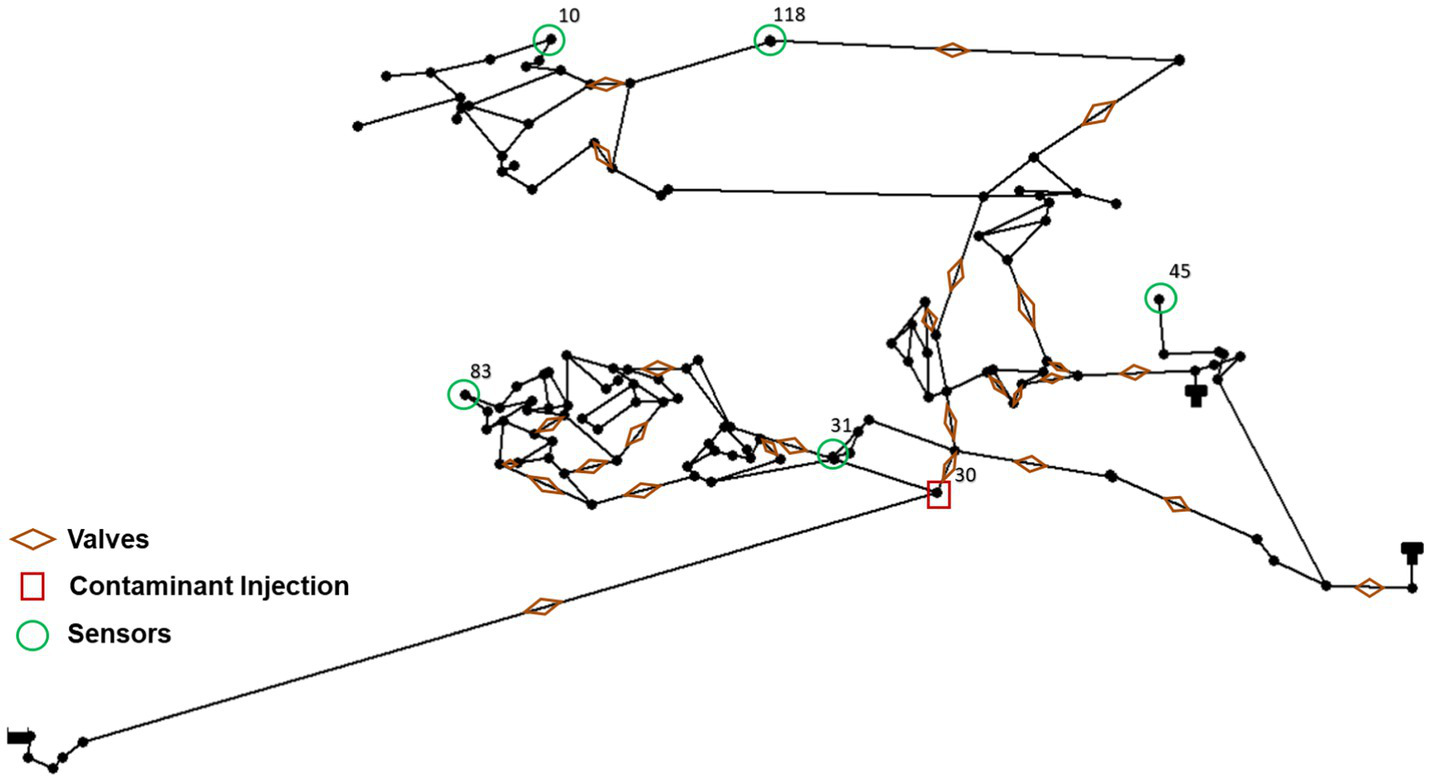
Layout of case study WDS BWSN.
Table 2
| Network | Type | ID |
|---|---|---|
| Net 3 | Valves (links) | ‘111’, ‘175’, ‘105’, ‘116’, ‘177’, ‘215’, ‘204’, ‘237’, ‘269’, ‘173’, ‘123’, ‘107’, ‘229’, ‘311’, ‘155’, ‘309’, ‘221’, ‘231’, ‘317’, ‘301’ |
| Hydrants (junctions) | ‘20,’ ‘40’, ‘50’, ‘60’, ‘601’, ‘61’, ‘120’, ‘129’, ‘164’, ‘169’, ‘173’, ‘179’, ‘181’, ‘183’, ‘184’, ‘187’, ‘195’, ‘204’, ‘206’, ‘208’, ‘241’, ‘249’, ‘257’, ‘259’, ‘261’, ‘263’, ‘265’, ‘267’, ‘269’, ‘271’, ‘273’, ‘275’ | |
| BWSN | Valves (links) | ‘0,’ ‘1’, ‘33’, ‘40’, ‘45’, ‘109’, ‘143’, ‘66’, ‘35’, ‘42’, ‘160’, ‘46’, ‘111’, ‘34’, ‘164’, ‘31’, ‘94’, ‘53’, ‘73’, ‘51’, ‘71’, ‘70’, ‘69’, ‘68’, ‘67’, ‘121’, ‘115’, ‘113’ |
| Hydrants (junctions) | ‘7,’ ‘9’, ‘13’, ‘14’, ‘16’, ‘21’, ‘24’, ‘26’, ‘29,’ ‘36’, ‘38’, ‘47’, ‘48’, ‘56’, ‘57’, ‘59’, ‘60’, ‘61’, ‘62’, ‘63’, ‘64’, ‘65’, ‘66’, ‘67’, ‘78’, ‘79’, ‘80’, ‘85’, ‘86’, ‘87’, ‘88’, ‘90’, ‘91’,'92′, ‘105’, ‘106’, ‘109’, ‘110’, ‘111’, ‘112’, ‘113’, ‘115’, ‘119’, ‘120’, ‘121’, ‘125’, ‘128’ |
Valve and hydrant IDs for both used water networks.
The valve layouts for both networks are sourced from the previous study by Preis and Ostfeld (2008). Hydrants are assigned a demand of zero until a flushing event occurs at a demand of 100 GPM (0.006308 m3/s). The Net3 system features a 24-h demand flow pattern, whereas the BWSN system features a 96-h demand flow pattern. Contaminant injection locations for Net3 and BWSN networks are at nodes 101 and node 30, respectively (Preis and Ostfeld, 2008). In both networks, the injection pattern is designed to form a uniform pattern starting at 8 a.m. and ending at 10 a.m. The EPANET source type was selected as a “set point booster” for both networks, with a fixed concentration of 50 mg/L for Net3, and 100 mg/L for BWSN.
The contamination early warning detection system (EWDS) in Net3 consists of five monitoring stations located at nodes 15, 35, 145, 225, and 255, while the EWDS in the BWSN network comprises five sensors placed at junctions 10, 31, 45, 83, and 118. The layout design was placed in a way that would increase the probability of detecting any random intrusion event (Preis and Ostfeld, 2008). Based on the contamination detection process, the BWNS sensor located at node 31 discovered the presence of contaminants at 08:25, while the Net3 sensor at node 35 detected contamination at 10:55. It is assumed that identifying the contamination source and stopping any further spread of contamination will take approximately 65 min. Furthermore, it is expected that determining the most optimal actions and initiating a response by deploying operational teams to address the contamination risk will require 1 h. As a result, the optimal consequence management response activities, which involve shutting off valves and turning on the hydrants, are estimated to begin at 13:00 for Net3 and 10:30 for BWSN.
3.2 Performance comparison of GP kernels
A key aspect of Bayesian optimization is the use of surrogate models to approximate the objective functions. Herein, we used Gaussian Processes (GPs) due to their flexibility and ability to quantify uncertainty. In GP regression, the covariance kernel defines how points in the input space are correlated with each other. This correlation is essential for making predictions about the objective functions at unsampled points based on the observations at sampled points. Here, we examined three different covariance kernel functions, namely Squared-Exponential (SE), Matérn 3/2 (M32), and Rational Quadratic (RQ) to find which MOBO method produces the best performance.
For each kernel, 25 initial points and 30 iterations were implemented. The choice of 30 iterations is based on the study by Galuzio et al. (2020), in which MOBO were systematically evaluated against several benchmark functions (Galuzio et al., 2020). The analysis showed that MOBO generally produced high-quality Pareto front approximations at 20 objective function evaluations, even for problems with various dimensionalities and constraints. Thus, a number of 30 iterations were selected in this study to ensure MOBO convergence. Additionally, for each one of the three covariance kernels, the MOBO optimization was performed 25 times, where each optimization run starts with a different set of 25 randomly generated initial points, followed by 30 optimization iterations. The Net3 WDS was selected for this analysis.
3.2.1 Execution time and number of Pareto solutions
In this study, execution time is defined as the duration of running the MOBO algorithm for the total of 55 objective function evaluations (25 initial + 30 iterations). The study was conducted using a VivoBook_ASUS Laptop featuring an Intel(R) Core i5-10th generation processor and 12 GB of RAM. As can be seen in Figure 6A, the M32 kernel exhibits the lowest median and average execution times, followed by those of SE and RQ, respectively. Furthermore, the variability in the execution times among the 25 optimization runs is the highest for the RQ kernel. Consequently, the results indicate that the M32 kernel outperforms other kernels in terms of efficiency and consistency. Figure 6B displays the number of optimal Pareto solutions (NOPS) obtained by each GP kernel. In general, the higher the NOPS, the better performance. The RQ covariance function produced a limited number of NOPS, while the M32 kernel produced the highest median NOPS value of all the kernels.
Figure 6

(a) Execution time, and (b) Number of Pareto Solutions, produced by different MOBO covariance kernels.
3.2.2 Quality of Pareto front
In addition to the execution time and number of Pareto solutions, it is important to assess the quality of the Pareto fronts generated by the algorithm. Although it is impossible to determine whether the proposed algorithm has reached the true optimum since the real Pareto-front is unknown, it is feasible to evaluate when the algorithm has produced high-quality Pareto fronts using various metrics. Herein, the hypervolume indicator and the diversity metric are employed to compare the quality of the solutions obtained by various covariance kernels. Figure 7 presents the estimated hypervolume and diversity metric values obtained after 30 iterations of the MOBO algorithm applied to the Net3 water network for 25 optimization runs. To compute the hypervolume, a reference point that exceeds the maximum value of the Pareto front must be selected. For Net3, a reference point representing 22 filed actions and 73 kg consumed contaminant mass was selected based on the obtained Pareto solutions values.
Figure 7

(a) Hypervolume, and (b) diversity metric values produced by different MOBO kernels.
As can be seen in Figure 7A, the M32 kernel displays the highest median and average, and lowest variability in hypervolume values. Figure 7B reveals that the diversity of all three kernels is somewhat comparable, with SE and M32 kernels generating solutions with slightly higher diversity distribution compared to the RQ kernel. However, the MOBO with SE kernel produced a slightly more evenly dispersed set of non-dominated solutions. Overall, the results suggest that the MOBO_M32 algorithm produces the most reliable outcomes, resulting in the highest quality solutions compared to the other kernels assessed.
3.2.3 Pareto front convergence
In order to assess the proximity of the estimated integer Pareto front to the continuous MOBO Pareto front, the GD and IGD indicators are employed. The performance of the kernel improves with a smaller distance between the two Pareto fronts. Figure 8A presents the results of the performance indicators for the MOBO algorithm using the tested kernels. Notably, the IGD metric provides a more comprehensive understanding than the GD indicator. In contrast to GD, IGD evaluates the distance between each point on the integer Pareto front and its nearest reference points on the continuous Pareto front, considering all points on the continuous Pareto front. Based on the outcomes of Figure 8B, it can be inferred that the M32 and RQ kernels’ results converge to the continuous MOBO Pareto front solutions, as demonstrated by their low GD and IGD values. M32 also displays the lowest IGD results.
Figure 8

(a) Generational distance, and (b) inverted generational distance of different kernels.
Overall, the M32 and RQ kernels exhibited strong performance indicators compared to the SE kernel. Taken together, the results of the sensitivity analyses revealed that MOBO with the M32 kernel function displays the best performance for the case study. The Integer MOBO Pareto front outcomes attained with the M32 kernel function demonstrated excellent convergence to the continuous Pareto front results, reasonable diversity point solutions, the best quality Pareto front solutions, and the highest number of point solutions. Consequently, the MOBO algorithm with the M32 kernel (MOBO_M32) is selected for further analysis throughout the remainder of this study.
3.3 Comparison against NSGA-II
Next, we compared the performance of the MOBO_M32 algorithm against the widely used NSGA-II algorithm. The parameters for NSGA-II were selected based on an earlier application for OORC in WDSs by Preis and Ostfeld (2008). Specifically, the probabilities of crossover and mutation were set at 0.75 and 0.07, respectively, and a total of 30 generations with a population size of 24 were selected (i.e., 720 iterations).
In Figure 9, the convergence profiles for the Net3 water network are presented for both the MOBO and NSGA-II algorithms. The red circles in the figure represent the estimated hypervolume values for each corresponding iteration in MOBO vs. NSGA-II. The results indicate that MOBO converges to a high-quality Pareto front within 27 iterations, after which no significant improvement is achieved by conducting more iterations. In contrast, NSGA-II demonstrates a sharp increase in performance for the first 250 iterations, followed by a steady improvement until it ultimately stalls near 650 function evaluations.
Figure 9
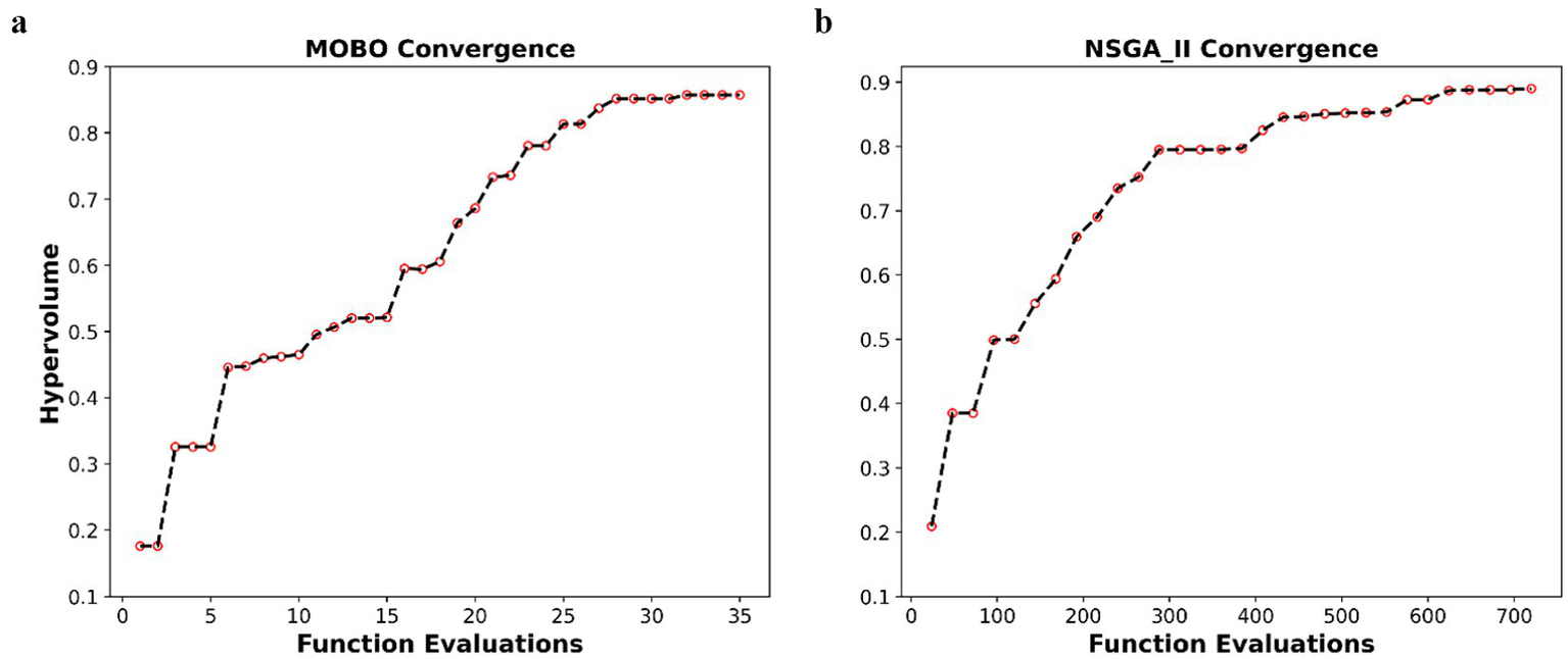
Convergence profiles for (a) MOBO and (b) NSGA-II.
We conducted several independent runs of the MOBO algorithm under a varying number of iterations. For all runs, the results indicated that increasing the number of evaluations generally enhanced the quality of the Pareto front. However, the MOBO algorithm consistently achieved a stable Pareto front after 25–30 iterations, with the hypervolume remaining relatively consistent afterward. This analysis confirmed the robustness and stability of the proposed MOBO algorithm.
The results show how fast MOBO converges to the optimal Pareto front compared to NSGA-II. It is important to note that each iteration for both algorithms requires a single evaluation of both objective functions. Thus, MOBO requires significantly fewer iterations to converge compared to NSGA-II. This highlights the significant advantage of implementing Bayesian optimization for the real-time optimization of operational response to contamination events in WDSs.
3.4 Effect of network size and complexity
To better understand how the size and complexity of the WDS affects the performance of the proposed MOBO framework, we compared the results of the two WDSs for both MOBO vs. NSGA-II.
Figure 10 shows the Pareto front solutions obtained by both algorithms of the number of field operations (f1) versus the contaminant mass consumed (f2) for both Net3 and BWSN.
Figure 10

Optimal Pareto front: consumed contamination mass f2 versus number of field operations f1. (A) MOBO on Net3; (B) NSGA-II on Net3; (C) MOBO on BWSN; (D) NSGA-II on BWSN.
As can be seen in the figure, if no actions were executed, EPANET simulation results revealed that up to 76 kg and 108 kg of contamination mass would have been consumed in Net3 and BWSN networks, respectively, during a simulation period of 24 h and 96 h, respectively.
Comparing the performance of MOBO_M32 and NSGA-II algorithms, it can be seen that the MOBO_M32 algorithm outperforms the NSGA-II algorithm in terms of total contamination reduction. Specifically, for Net3, the MOBO_M32 algorithm achieved a 76% reduction in contamination using 17 field operations as illustrated in Figure 10A, whereas the NSGA-II algorithm accomplished a 69% reduction using the same number of operations as demonstrated in Figure 10B. Similarly, for the BWSN network, the MOBO_M32 algorithm achieved a 91% reduction in contamination by executing 20 valve closings and hydrant openings as shown in Figure 10C. In comparison, the NSGA-II algorithm accomplished an 84% reduction in contamination by performing the same number of field operations as illustrated in Figure 10D. Overall, these findings suggest that the MOBO_M32 algorithm yields better solutions than those produced by the NSGA-II algorithm.
Comparative analysis of the performance of NSGA-II and MOBO_M32 algorithms in terms of the whole Pareto front quality reflects that the NSGA-II algorithm slightly outperforms the MOBO_M32 algorithm. Specifically, the hypervolume values estimated from the Pareto front obtained by the genetic algorithm are 0.89 and 0.98 for Net3 and BWSN water networks, respectively (Figures 10B,D), which are slightly higher than the hypervolume values obtained by the MOBO_M32 algorithm that are 0.85 and 0.92 for Net3 and BWSN water networks, respectively (Figures 10A,C). However, when comparing the Pareto front results of Figure 10A to those of Figure 10B, the MOBO_M32 algorithm achieved better contamination reduction after six field operations, whereas NSGA-II achieved outstanding contamination reduction between three and six operations. Similarly, the MOBO_M32 algorithm showed better contamination reduction after the tenth operation, while NSGA-II outperformed it before the tenth action in the case of BWSN (as shown in Figures 10C,D).
A practical solution for the management of water networks involves the implementation of seven specific actions for the Net3 water network and 10 actions for the BWSN water network. For the Net3 water network, the recommended actions include opening hydrants number 259, 249, and 269, as well as closing valves number 111, 229, and 204. In the case of the BWSN water network, the suggested actions consist of opening hydrants number 38, 24, 57, 91, and 68, as well as closing valves number 42, 51, 143, 109, and 33. This selection aims to balance operational efforts with a significant reduction in contamination.
The average time required to obtain the optimal Pareto front for the Net3 water network was approximately 1.15 min using the MOBO_M32 algorithm and 7.50 min using NSGA-II. The total elapsed time for the BWSN water network was 2.45 and 25.43 min for the MOBO_M32 algorithm and NSGA-II, respectively. The overall computational time includes both the EPANET simulation time and the algorithm running time for each evaluation. NSGA-II took approximately 10 times longer than the MOBO_M32 algorithm because its total computing time comprises the EPANET simulation running time for each multi-objective chromosome, multiplied by the size of the population and, by then, the number of NSGA-II generations. The MOBO_M32 algorithm required only 30 iterations to generate the optimal Pareto fronts shown in Figure 10. Therefore, MOBO_M32 is particularly useful when dealing with more complex water networks. The proposed algorithm demonstrated superior performance in identifying optimal solutions with a significantly shorter computation time than NSGA-II. Consequently, the MOBO_M32 algorithm is highly recommended as a promising tool for optimizing water distribution network design and management.
4 Conclusion
Contamination of treated drinking water is a significant public health and safety concern. This study introduces a multi-objective Bayesian optimization (MOBO) framework aimed at optimizing the operational response to contamination incidents in drinking water distribution systems (WDSs). The framework seeks to optimize the conflicting objectives of reducing response time while improving water quality metrics after contamination. To achieve this, two objectives were concurrently optimized: the number of field operations (closing valves and opening hydrants) and the total mass of contaminants consumed.
A sensitivity analysis was carried out to select the MOBO algorithm’s hyperparameters, including the covariance kernel of the surrogate model. The efficacy of the framework was illustrated through a case study involving two WDSs with varying sizes and complexities. Moreover, the performance of the MOBO algorithm was evaluated against the commonly used NSGA-II algorithm.
Taken together, the results demonstrated that the MOBO framework can effectively determine optimal response actions, swiftly and efficiently enhancing water quality following contamination events in WDSs. Comparing the performance of various covariance functions using multiple performance indicators revealed that MOBO with the Matern kernel consistently performed better than other kernels, as measured by convergence, spread, and the number of non-dominated solutions. Convergence analysis confirmed that the proposed MOBO algorithm converged to high-quality Pareto front solutions, requiring significantly fewer evaluations of the objective functions than NSGA-II.
While the results of the two case study WDSs demonstrated the potential of the MOBO framework for optimizing contamination response in WDSs of different sizes and complexities, scaling the proposed framework to larger and more complex WDSs might present several challenges. The increased complexity of the models and the larger number of decision variables can significantly affect the computational cost of both individual simulations and the overall optimization process. Future research could explore strategies to address these challenges, including dimensionality reduction, using advanced GP models such as sparse GP or hierarchical GP, and implementing parallelization techniques to speed up both the simulation runs and the GP training process.
Statements
Data availability statement
The raw data supporting the conclusions of this article will be made available by the authors, without undue reservation.
Author contributions
KA: Conceptualization, Formal analysis, Investigation, Methodology, Software, Validation, Visualization, Writing – original draft. AA: Conceptualization, Funding acquisition, Project administration, Resources, Supervision, Writing – review & editing.
Funding
The author(s) declare that financial support was received for the research and/or publication of this article. Funding provided for this effort by the DoD Environmental Security Technology Certification Program (ESTCP) under project number EW23-7798 is gratefully acknowledged.
Conflict of interest
The authors declare that the research was conducted in the absence of any commercial or financial relationships that could be construed as a potential conflict of interest.
Generative AI statement
The authors declare that no Gen AI was used in the creation of this manuscript.
Publisher’s note
All claims expressed in this article are solely those of the authors and do not necessarily represent those of their affiliated organizations, or those of the publisher, the editors and the reviewers. Any product that may be evaluated in this article, or claim that may be made by its manufacturer, is not guaranteed or endorsed by the publisher.
References
1
Alfonso L. Jonoski A. Solomatine D. (2010). Multiobjective optimization of operational responses for contaminant flushing in water distribution networks. J. Water Resour. Plan. Manag.136, 48–58. doi: 10.1061/(ASCE)0733-9496(2010)136:1(48)
2
Alnajim K. Abokifa A. A. (2024). Bayesian optimization for contamination source identification in water distribution networks. Water16:168. doi: 10.3390/w16010168
3
Aral M. M. Guan J. Maslia M. L. (2010). Optimal design of sensor placement in water distribution networks. J. Water Resour. Plan. Manag.136, 5–18. doi: 10.1061/(asce)wr.1943-5452.0000001
4
Baranowski T. M. Leboeuf E. J. (2008). Consequence management utilizing optimization. J. Water Resour. Plan. Manag.134, 386–394. doi: 10.1061/(ASCE)0733-9496(2008)134:4(386)
5
Bashi-Azghadi S. N. Afshar M. H. Afshar A. (2017). Multi-objective optimization response modeling to contaminated water distribution networks: pressure driven versus demand driven analysis. KSCE J. Civil Eng.21, 2085–2096. doi: 10.1007/S12205-017-0447-7
6
Bazargan-Lari M. R. (2018). Real-time response to contamination emergencies of urban water networks. Iran. J. Sci. Technol. Trans. Civil Eng.42, 73–83. doi: 10.1007/S40996-017-0071-2/TABLES/3
7
Blank J. Deb K. (2020). Pymoo: multi-objective optimization in python. Ieee access8, 89497–89509. doi: 10.1109/ACCESS.2020.2990567
8
Brochu E. Cora V. M. De Freitas N. (2010). A tutorial on Bayesian optimization of expensive cost functions, with application to active user modeling and hierarchical reinforcement learning. arXiv. doi: 10.48550/arxiv.1012.2599
9
Candelieri A. Perego R. Archetti F. (2018). Bayesian optimization of pump operations in water distribution systems. J. Glob. Optim.71, 213–235. doi: 10.1007/s10898-018-0641-2
10
Coello Coello C. A. Reyes Sierra M. (2004). “A study of the parallelization of a coevolutionary multi-objective evolutionary algorithm” in Lecture notes in artificial intelligence (subseries of lecture notes in computer science). eds. OkadaM.SatohI. (Berlin, Heidelberg: Springer), 688–697.
11
Daulton S. Eriksson D. Balandat M. Bakshy E. (2022). “Multi-objective bayesian optimization over high-dimensional search spaces,” in Uncertainty in Artificial Intelligence, 507–517. PMLR.
12
Deb K. Pratap A. Agarwal S. Meyarivan T. (2002). A fast and elitist multiobjective genetic algorithm: NSGA-II. IEEE Trans. Evol. Comput.6, 182–197. doi: 10.1109/4235.996017
13
Fonseca C. M. Paquete L. López-Ibánez M. (2006). “An improved dimension-sweep algorithm for the hypervolume indicator” in IEEE international conference on evolutionary computation. eds. ShiY.EberhartR. (Piscataway, NJ: IEEE), 1157–1163.
14
Galuzio P. P. de Vasconcelos Segundo E. H. Coelho L. D. S. Mariani V. C. (2020). MOBOpt — multi-objective Bayesian optimization. SoftwareX12:100520. doi: 10.1016/j.softx.2020.100520
15
Grbčić L. Lučin I. Kranjčević L. Družeta S. (2020). Water supply network pollution source identification by random forest algorithm. J. Hydroinf.22, 1521–1535. doi: 10.2166/HYDRO.2020.042
16
Hu C. Cai J. Zeng D. Yan X. Gong W. Wang L. (2020). Deep reinforcement learning based valve scheduling for pollution isolation in water distribution network. Math. Biosci. Eng.17, 105–121. doi: 10.3934/mbe.2020006
17
Hu C. Yan X. Gong W. Liu X. Wang L. Gao L. (2020). Multi-objective based scheduling algorithm for sudden drinking water contamination incident. Swarm. Evol. Comput.55:100674. doi: 10.1016/j.swevo.2020.100674
18
Hu C. Zhao J. Yan X. Zeng D. Guo S. (2015). A MapReduce based parallel niche genetic algorithm for contaminant source identification in water distribution network. Ad Hoc Netw.35, 116–126. doi: 10.1016/j.adhoc.2015.07.011
19
Klise K. Hart D. Moriarty D. (2017). Water network tool for resilience (WNTR) user manual. Albuquerque, NM: Sandia National Lab.
20
Laird C. D. Biegler L. T. van Bloemen Waanders B. G. Bartlett R. A. (2005). Contamination source determination for water networks. J. Water Resour. Plan. Manag.131, 125–134. doi: 10.1061/(asce)0733-9496(2005)131:2(125)
21
Melkumyan A. Nettleton E. (2009). “An observation angle dependent nonstationary covariance function for Gaussian process regression” in Lecture notes in computer science (including subseries lecture notes in artificial intelligence and lecture notes in bioinformatics). eds. DorigoM.BirattariM. (Cham: Springer), 331–339.
22
Moeini M. Sela L. Taha A. F. Abokifa A. A. (2023). Bayesian optimization of booster disinfection scheduling in water distribution networks. Water Res.242:120117. doi: 10.1016/j.watres.2023.120117
23
Mu T. Huang M. Tang S. Zhang R. Chen G. Jiang B. (2022). Sensor partitioning placements via random walk and water quality and leakage detection models within water distribution systems. Water Resour. Manag.36, 5297–5311. doi: 10.1007/s11269-022-03312-z
24
Ostfeld A. Salomons E. (2004). Optimal layout of early warning detection stations for water distribution systems security. J. Water Resour. Plan. Manag.130, 377–385. doi: 10.1061/(ASCE)0733-9496(2004)130:5(377)
25
Pandey J. Srinivas V. V. (2024). Integrated sustainability index for assessing the performance of water distribution network. Water Resour. Manag.38, 3707–3724. doi: 10.1007/s11269-024-03835-7
26
Park S. Na J. Kim M. Lee J. M. (2018). Multi-objective Bayesian optimization of chemical reactor design using computational fluid dynamics. Comput. Chem. Eng.119, 25–37. doi: 10.1016/j.compchemeng.2018.08.005
27
Ponti A. Candelieri A. Archetti F. (2021). A new evolutionary approach to optimal sensor placement in water distribution networks. Water13:1625. doi: 10.3390/W13121625
28
Poulin A. Mailhot A. Grondin P. Delorme L. Periche N. Villeneuve J.-P. (2008). Heuristic approach for operational response to drinking water contamination. J. Water Resour. Plan. Manag.134, 457–465. doi: 10.1061/ASCE0733-94962008134:5457
29
Poulin A. Mailhot A. Grondin P. Delorme L. Villeneuve J. P. (2006). Optimization of operational response to contamination in water networks. Annual Water Distrib. Syst. Anal.2006, 1–15. doi: 10.1061/40941(247)117
30
Poulin A. Mailhot A. Nathalie Periche L. Villeneuve J.-P. (2010). Planning unidirectional flushing operations as a response to drinking water distribution system contamination. J. Water Resour. Plan. Manag.136, 647–657. doi: 10.1061/ASCEWR.1943-5452.0000085
31
Preis A. Ostfeld A. (2006). Contamination source identification in water systems: a hybrid model trees–linear programming scheme. J. Water Resour. Plan. Manag.132, 263–273. doi: 10.1061/(asce)0733-9496(2006)132:4(263)
32
Preis A. Ostfeld A. (2008). Multiobjective contaminant response modeling for water distribution systems security. J. Hydroinf.10, 267–274. doi: 10.2166/HYDRO.2008.061
33
Rasekh A. Brumbelow K. (2014). Drinking water distribution systems contamination management to reduce public health impacts and system service interruptions. Environ. Model Softw.51, 12–25. doi: 10.1016/j.envsoft.2013.09.019
34
Rasekh A. Brumbelow K. (2015). A dynamic simulation–optimization model for adaptive management of urban water distribution system contamination threats. Appl. Soft Comput.32, 59–71. doi: 10.1016/J.ASOC.2015.03.021
35
Rathi S. Gupta R. (2016). A simple sensor placement approach for regular monitoring and contamination detection in water distribution networks. KSCE J. Civ. Eng.20, 597–608. doi: 10.1007/S12205-015-0024-X/METRICS
36
Shafiee M. E. Berglund E. Z. (2015). Real-time guidance for hydrant flushing using sensor-hydrant decision trees. J. Water Resour. Plan. Manag.141:04014079. doi: 10.1061/(asce)wr.1943-5452.0000475
37
Shahsavandi M. Yazdi J. Jalili-Ghazizadeh M. Mehrabadi A. R. (2024). A rule-based water quality sensor placement method for water supply systems using network topology. Water Resour. Manag.38, 569–586. doi: 10.1007/s11269-023-03685-9
38
Shu L. Jiang P. Shao X. Wang Y. (2020). A new multi-objective bayesian optimization formulation with the acquisition function for convergence and diversity. J. Mech. Design Trans. ASME142:46508. doi: 10.1115/1.4046508
39
Van Veldhuizen D. A. Lamont G. B. (1998). “Evolutionary computation and convergence to a pareto front” in Late breaking papers at the genetic programming 1998 conference. ed. LangdonW. (England: University of Birmingham.), 221–228.
40
Williams C. K. I. Rasmussen C. E. (2006). Gaussian processes for machine learning. Cambridge, MA: MIT press.
41
Wu W. Wei Z. Wu L. (2024). Public satisfaction with water quality under the implementation of water quality monitor standard system. Water Resour. Manag.38, 4197–4212. doi: 10.1007/s11269-024-03859-z
42
Yang X. Boccelli D. L. (2014). Bayesian approach for real-time probabilistic contamination source identification. J. Water Resour. Plan. Manag.140:04014019. doi: 10.1061/(asce)wr.1943-5452.0000381
43
Yusoff Y. Ngadiman M. S. Zain A. M. (2011). Overview of NSGA-II for optimizing machining process parameters. Procedia Eng.15, 3978–3983. doi: 10.1016/j.proeng.2011.08.745
Summary
Keywords
Bayesian optimization, contamination response, multi-objective optimization, water distribution, drinking water
Citation
Alnajim K and Abokifa AA (2025) Operational response to contamination in water distribution systems: a multi-objective Bayesian optimization approach. Front. Water 7:1547112. doi: 10.3389/frwa.2025.1547112
Received
17 December 2024
Accepted
28 April 2025
Published
23 May 2025
Volume
7 - 2025
Edited by
Surjeet Dalal, Amity University Gurgaon, India
Reviewed by
Jiangjiang Zhang, Hohai University, China
Shweta Rathi, National Institute of Technology, Kurukshetra, India
Brian Barkdoll, Michigan Technological University, United States
Updates
Copyright
© 2025 Alnajim and Abokifa.
This is an open-access article distributed under the terms of the Creative Commons Attribution License (CC BY). The use, distribution or reproduction in other forums is permitted, provided the original author(s) and the copyright owner(s) are credited and that the original publication in this journal is cited, in accordance with accepted academic practice. No use, distribution or reproduction is permitted which does not comply with these terms.
*Correspondence: Ahmed A. Abokifa, abokifa@uic.edu
Disclaimer
All claims expressed in this article are solely those of the authors and do not necessarily represent those of their affiliated organizations, or those of the publisher, the editors and the reviewers. Any product that may be evaluated in this article or claim that may be made by its manufacturer is not guaranteed or endorsed by the publisher.