Abstract
Long short-term memory (LSTM) networks have become indispensable tools in hydrological modeling due to their ability to capture long-term dependencies, handle non-linear relationships, and integrate multiple data sources but suffer from limited interpretability due to their black box nature. To address this limitation, we propose an explainable module within the LSTM framework, specifically designed for flood prediction across 531 catchments in the contiguous United States. Our approach incorporates a simplified gated module, which is interposed between the input data and the LSTM network, providing a transparent view of the module’s pattern recognition process. This gated module allows for easy identification of key variables and optimal lookback windows, and clusters the gated information into four categories: short-term and long-term impacts of precipitation and temperature. This categorization enhances our understanding of how the module utilizes input data and reveals underlying mechanisms in flood prediction. The modular design of our approach demonstrates high correlation with Saliency method, validating the credibility of its explanatory mechanisms, providing comparable interpretability features to LSTMs while illuminating key variables and optimal lookback windows considered most informative by hydrological models, and opening up new avenues for AI-assisted scientific discovery in the field.
Highlights
An explainable module based on the LSTM framework has been developed specifically for flood prediction.
The module identifies key variables and the optimal time windows through intuitive visualization.
The module demonstrates high correlation with saliency method, validating the credibility of its explanatory mechanisms.
1 Introduction
Streamflow estimation is essential for various applications, including flood hazards mitigation (Alfieri et al., 2018), water sustainability studies (McDonnell et al., 2018; Zhang et al., 2023), reservoir management (Beça et al., 2023), and humanitarian aid supports (Altay and Narayanan, 2022). The fundamental challenge in streamflow prediction lies in elucidating the hydrological mechanisms and establishing the relationship between various variables and streamflow, which are often characterized by dynamic complexity and non-stationarity (Coulibaly and Baldwin, 2005; Nourani, 2017). The most common method for forecasting streamflow is process-based hydrological modeling which facilitates an understanding of the physical processes involved in runoff generation and routing (Li et al., 2013). However, these models rely on simplifying assumptions and require substantial input data (Danandeh Mehr et al., 2013). An alternative approach is the use of data-driven models, which can quickly adapt to new conditions and are efficient in handling large datasets (Liu et al., 2015; Pokharel et al., 2023; Wilbrand et al., 2023). Currently, statistical and machine learning (ML) methods, both falling under the category of data-driven models, are widely used to develop predictive and analytical systems. Compared to statistical models that struggle to capture the nonlinear and nonstationary patterns inherent in time series (Han et al., 2024; Li et al., 2024), ML excels at extracting implicit patterns from high-dimensional, nonlinear, and multivariate data in complex and dynamic environments (Hussain et al., 2020; Herath et al., 2021; Yao et al., 2023; Tripathy and Mishra, 2024).
ML techniques have been increasingly applied in the hydrometeorological field (Zhu et al., 2020; Ditthakit et al., 2021; Ma et al., 2021; Mohammadi et al., 2022; Du et al., 2023). Among them, Long Short-Term Memory (LSTM) networks have demonstrated significant skills in estimating streamflow (Hochreiter and Schmidhuber, 1997; Greff et al., 2017; Kratzert et al., 2018; Van Houdt et al., 2020). For instance, Kratzert et al. (2019) showed that the LSTM model significantly improved the prediction of the rainfall-runoff process compared to several different hydrological benchmark models, such as the Variable Infiltration Capacity (VIC) model. Current research primarily focuses on enhancing model accuracy by integrating operational data or refining model components. Kwon et al. (2023) integrated reservoir operational data into a LSTM model for streamflow prediction, resulting in an increase in the Nash-Sutcliffe Efficiency (NSE) values ranging from 0.18 to 0.21. Ni et al. (2020) utilized wavelet and convolutional modules to enhance the LSTM model for predicting streamflow and rainfall. Wang et al. (2023) incorporated a Convolutional Neural Network (CNN) followed by the application of a LSTM model to simulate runoff, resulted in a marked enhancement in model accuracy. Nonetheless, ML is difficult to interpret, leading them to be termed “black boxes” (Shen, 2018). This lack of transparency can undermine trust, hinder informed decision-making, and pose challenges in regulatory and ethical contexts. Therefore, conducting research on the explainability of ML models is essential.
Interpretability is often associated with understanding the causal relationship between the model’s input and output, providing insights into the model’s reasoning process (Adadi and Berrada, 2018). Interpretability methods can be broadly categorized into three principal approaches. First, the direct analysis of hidden states such as memory cells (Kratzert et al., 2018; Kratzert et al., 2019) and attention module (Ding et al., 2020) scrutinize the model’s internal representations to understand its decision-making processes. Second, gradient-based methods, exemplified by the Layer-wise Relevance Propagation technique (Arras et al., 2019), utilize backpropagation to quantify the contribution of each input feature to the model’s predictions. Lastly, perturbation-based analysis, including variable contribution measures, cumulative local effect diagrams, SHapley Additive exPlanations, partial dependence profiles, individual conditional explanations, and local interpretable model-agnostic explanations (Althoff et al., 2021; Núñez et al., 2023), assess the model’s sensitivity to input changes by observing the variations of the output, thereby indicating the predictive influence.
Despite the focus of direct analysis of hidden states on visualization, gradient-based methods on model computation, and perturbation-based analyses on input data, there is a gap regarding the integration of these approaches to develop a straightforward, visually oriented method that considers the interaction between input data and model. Such a method is essential to explore the rationale behind hydrological predictions, particularly which variables and time periods within the time series data are most influential and their specific roles in the decision-making process. In this study, we introduce a module designed to explore the potential of the explanatory ML to advance scientific understanding of hydrological processes, with a focus on identifying data choices for models. LSTM-based models are established individually for 531 catchments across the contiguous United States. With a simple visible gated weights module adopted, we analyze the evolution of temporal information hidden in the networks, and reveal model behaviors in predicting streamflow from this information.
2 Materials and methods
2.1 Catchment attributes and meteorology for large-sample studies (CAMELS) data
The CAMELS dataset, introduced by Addor et al. (2017) and Newman et al. (2015), is utilized for training and evaluating the LSTM model in this study. This dataset contains hydrometeorological time series observations over 671 reference basins across the contiguous United States. However, it should be noted that certain basins exhibit a significant (>10%) discrepancy in the calculation of their basin areas, which introduces considerable uncertainties in modeling studies. As a result, these basins with substantial discrepancies are excluded from the analysis, leaving only 531 basins with catchment areas smaller than 2000 km2 from the CAMELS dataset as shown in Figure 1. This selection of basins aligns with the approach adopted by Newman et al. (2017) and Kratzert et al. (2019) in their respective studies.
Figure 1

Reference basins used in this study. The basins are represented by dots, with color intensity indicating the slope gradient and dot size reflecting the basin area.
Three different types of meteorological forcing data are included in CAMELS. For this study, the Daily Surface Weather Data on a 1-km Grid for North America is used. The input data for the study includes the following variables for the 30 days prior to the predicted day: daily streamflow (SF), cumulative precipitation (PRE), average short-wave radiation (RAD), maximum air temperature (Tmax), minimum air temperature (Tmin), and average vapor pressure (VP). Prior to model calculation, all inputs are normalized by utilizing the respective maximum and the minimum values. The model output is daily streamflow. Since the models are trained individually for each station, the static attributes (e.g., typography) of the basins are not included as predictors in the model. The choice to train on a single station was primarily to capture local hydrological characteristics and dynamic changes more precisely, while avoiding biases caused by regional differences. The models are trained using the daily data during a 10-year period from October 1st, 1989, to September 30th, 1999, and tested using another 10-year data from October 1st, 1999 to September 30th, 2009.
2.2 Deep learning model
The deep-learning algorithm used in this study is shown as Figure 2. The model comprises a gated module, a LSTM module, and a prediction module. Firstly, a gated layer is employed to extract the gated information, which controls the passing weight of each input variable. Subsequently, the gated information is then fed into the traditional LSTM module. Finally, a predict module with two Fully Connected Neural Network (FCNN) layers, comprising 32 and 1 neuron, respectively, and using a Leaky ReLU activation function, are utilized to predict the streamflow.
Figure 2

The deep learning model architecture utilized in this study.
2.2.1 Input data format
Each group of input data, excluding SF, such as PRE, RAD, Tmax, Tmin, and VP, undergoes a gated information calculation prior to being integrated into the LSTM module. The input data originate as 2D grids but are transformed into a 1D time series by calculating the watershed average for each variable over the study area. For instance, for PRE, the mean value across all grid cells within the watershed at each time step is computed, resulting in a single time series. This process is repeated for SF, RAD, Tmax, Tmin, and VP, yielding six distinct time series. These six time series, each spanning 30 time steps, are then combined into a 6×30 matrix X. Each row of X represents one of the six variables, and each column represents a time step. To determine the optimal look-back window, preliminary experiments were conducted with different window sizes. Results indicated that extending the look-back window beyond 30 days did not consistently improve model accuracy across all stations. Hence, a 30-day look-back window was selected as a balanced compromise, effectively capturing both short-term dynamics and long-term dependencies while maintaining computational efficiency.
2.2.2 Gated module
In order to focus on the selection of model input data using gated information for subsequent model calculations, a gated layer is specifically designed to facilitate this process between the input variables and the LSTM module. The gating layer computes a feature matrix G∈R6 × 30 for the input matrix X, where each element indicates the relative importance of the corresponding input variable at each time step: a value of 0 indicates that the corresponding information is completely disregarded and has no impact on the model; a value closer to 1 signifies that the model absorbs a greater amount of information from the input. The computation involves the following steps:
-
Weight initialization
Each input variable xi,t (where i = 1,2, …, 6, t = 1,2, …, 30) is assigned an initial weight, which is learned during training.
-
Gating transforms
The initial weights are derived from the input matrix X through a gating transformation, resulting in the matrix Y. This transformation is defined as Equation 1:
Where Wg is the weight matrix, bg is the bias term, and σ denotes the sigmoid function. The sigmoid activation function ensures that all elements in matrix Y fall within the range [0, 1], which allows them to serve as appropriate weighting factors in subsequent calculations.
-
Self-attention mechanism
The inclusion of a self-attention mechanism is motivated by the need to enhance interactions not only across time but also between different hydrological variables. While LSTMs are capable of capturing long-term temporal dependencies, they may not fully leverage the intricate relationships between variables, especially in complex hydrological systems. The attention mechanism can improve the model’s ability to identify and weigh the importance of specific time steps and variables (Chen et al., 2025). This selective focus on relevant temporal patterns and variable interactions leads to improved predictive accuracy compared to baseline models without attention (Section 2.2.5).
The self-attention mechanism captures the temporal dependencies and interactions among different input variables. It performs point-wise multiplication with the input matrix Y, ensuring that each pixel point engages in a synergistic fusion with its counterparts across both spatial and temporal scales. This augmentation transcends the limitations of isolated information representation and preserves the fidelity of the original input data’s informational content. Specifically, given the input matrix Y, the self-attention mechanism computes attention as follows:
Firstly, generate Query (Q), Key (K), and Value (V) matrices as Equation 2:
Where WQ, WK, WV are learnable weight matrices. Secondly, compute attention scores using dot-product and scale as Equation 3:
Where d is the dimension of the matrix K. Finally, compute the output matrix as a weighted sum of values as Equation 4:
-
Element-wise multiplication
The computed weight matrix O is applied to the input matrix X via element-wise multiplication as Equation 5:
Where W represents the gated output matrix with the same dimensions as the input matrix X.
Empirical experimentation has substantiated that situating the self-attention mechanism after the gating layer is more conducive to preserving the intrinsic spatiotemporal characteristics of the original data. Premising the self-attention mechanism on the input data directly would imply an interaction that may not fully encapsulate these characteristics. By applying the self-attention mechanism to the gated output, the model can better leverage the learned control weights, ensuring robust and consistent behavior across diverse input conditions. The gating mechanism steadfastly preserves the learned control weights invariant, irrespective of the input state to which it is applied. This ensures that the model maintains a consistent and reliable performance across various scenarios, enhancing its overall robustness.
2.2.3 LSTM module
The output from the previous module, denoted as the weight matrix W∈R6 × 30, serves as the input to the LSTM module. The LSTM module processes this input sequentially over time steps, capturing temporal dependencies and long-term patterns in the data. Below is the detailed computation process of the LSTM module.
At each time step t, the LSTM cell updates its hidden state ht and cell state ct using the following as Equations 6–11:
Where Wt is the input vector at time step t; ht is the hidden state at time step t; ct is the cell state at time step t; ft, ot, it are the forget gate, input gate, and output gate activations, respectively; is the candidate cell state; Wf, Wi, Wc, Wo are the weight matrices for the gates and cell state; bf, bi, bc, bo are the bias terms.
The LSTM processes the 30 time steps sequentially, updating the hidden state ht and cell state ct at each step. The final hidden state h30 captures the temporal information across all 30 time steps, which is used as the output of the LSTM module.
2.2.4 Prediction module
The prediction module consists of two FCNN layers to predict the streamflow from the final hidden state h30. The computation is as Equations 12, 13:
Where W1, W2 are the weight matrix for the FCNN layers, b1, b2 are the bias terms. The output is the final prediction of the model, representing the estimated streamflow.
2.2.5 Optimized design
To ensure optimal performance, several key hyperparameters were carefully calibrated through preliminary experiments conducted on a randomly selected station, allowing to establish a robust foundation for the subsequent comprehensive analysis. The model was implemented using Python 3.8.2 and PyTorch 1.9.0 on a GeForce RTX 3090 GPU. An Adam optimizer with a mean square error (MSE) loss function was employed to minimize prediction errors. The initial learning rate was set to 0.01 and reduced by one-tenth if the test dataset loss did not decrease for three consecutive epochs. Training was halted if the learning rate dropped to 0.00001, or after a maximum of 100 epochs to ensure convergence without excessive computation. A weight decay rate of 0.0001 was applied to prevent overfitting. The batch size was chosen based on computational efficiency and memory constraints, ensuring stable training while maintaining model performance. The number of hidden units in the LSTM module was determined through grid search to balance model complexity and predictive accuracy. These hyperparameter configurations are summarized in Table 1, along with their corresponding performance metric improvement.
Table 1
| Hyperparameter | Baseline setting | Optimized value | Performance metric improvement (MSE %) |
|---|---|---|---|
| Learning rate | 0.001 | 0.01 (initial, reduced by 1/10 if no improvement) | 26 |
| Batch size | 64 | 64 | 3.2 |
| Number of hidden units | 64 | 128 | 33 |
| Number of epochs | 50 | 100 (max) | 17 |
| Weight decay | 0.001 | 0.0001 | 1.3 |
| Activation function | ReLU | Leaky ReLU | 0.9 |
| Optimizer | SGD | Adam | 3.0 |
| Early stopping criterion | None | LR < 0.00001 or no improvement for 3 epochs | 34 |
| Adding self-attention mechanism | None | Self-attention | 42 |
| Number of FCNN layers | 1 | 2 | 33 |
Hyperparameter configurations and corresponding performance metrics.
The baseline settings represent the initial configurations before hyperparameter tuning, while the optimized values were determined through grid search and cross-validation to minimize the MSE and improve model performance.
2.3 Evaluation of modeling performance
2.3.1 Instructive days
As outlined in Section 2.2.2, the model incorporates a gated layer to dynamically control the flow of information from input variables into subsequent computations. To gain deeper insights into the role of this gated mechanism, we introduce the concept of instructive days, which represents the size of the lookback window that effectively conveys useful temporal information for each variable in streamflow prediction. The analysis of instructive days provides insights into how the model prioritizes and utilizes different temporal information windows for each variable, shedding light on the overall information processing dynamics within the model. A larger number of instructive days indicates that the variable’s long-term information plays a crucial role in model inference. Conversely, a smaller number suggests that only information from a short period is necessary for the variable, and long-term information may not be as influential.
2.3.2 Clustering analysis
To explore the differences in state information conveyed by the gated mechanism, clustering analysis is adopted on the gated information based on the concept of instructive days. This approach aims to group variables according to their temporal influence and reveal patterns in how the model utilizes short-term versus long-term information.
Initially, the gated information for each variable is projected onto one-dimensional feature vectors. These vectors represent the variable type (e.g., SF, PRE, RAD, Tmax, Tmin, VP) and encode the temporal dependencies of the variable. This projection simplifies the representation while retaining the key characteristics of the gated information. From these projected feature vectors, two main features are selected for further classification: one captures the size of the lookback window (instructive days) that effectively contributes to streamflow prediction, and the other reflects the relative importance of the variable within the gated mechanism, indicating its overall impact on the model’s predictions.
Subsequently, the k-means clustering algorithm is applied using scikit-learn v1.3.0 package to aggregate the projected features into two distinct clusters. Specifically, each feature vector is treated as a data point in the two-dimensional feature space defined by the selected features. The k-means algorithm partitions the data points into two clusters based on their similarity in terms of temporal span and contribution magnitude. The resulting clusters highlight variables with similar temporal dynamics, distinguishing between those that primarily rely on short-term trends and those that leverage long-term dependencies.
2.3.3 Performance measures
Three performance measures are used to qualitatively evaluate the performance of the models: MSE, Pearson correlation coefficient (CC), and NSE. They are calculated as Equations 14–16:
Where N is the number of evaluation pair, Y is the modeled value, and X is the corresponding reference value. The optimum value of CC and NSE is 1, while 0 for MSE.
2.3.4 Explainable methods
To validate the credibility of the interpretability mechanisms in the proposed gated approach, two complementary attribution methods—saliency maps and feature ablation—are employed for comparative analysis.
-
Saliency maps
Saliency maps provide a straightforward approach for attributing importance to input features in neural networks. This method calculates the gradient of the output with respect to each input, revealing which input features most strongly influence the model’s predictions. Mathematically, this involves computing the partial derivatives of the output with respect to each input dimension. The magnitude of these gradients indicates how sensitive the output is to changes in the corresponding input feature. For deeper theoretical insights into gradient-based feature attribution, these can be found in Baehrens et al. (2009).
-
Feature ablation
Feature ablation quantifies feature importance by systematically replacing input values with baselines and measuring output changes. This perturbation-based method can evaluate individual features or feature groups collectively. In implementation, each feature’s values are independently replaced while observing prediction impacts (Kokhlikyan et al., 2020). Features causing significant error increases when modified are deemed important, indicating model reliance; conversely, features whose permutation does not affect predictions are considered unimportant. The procedure follows a structured approach: first calculating baseline error with original data, then systematically permuting each feature while measuring resulting error changes, and finally ranking features by their impact on model performance. This methodology provides an interpretable, quantitative assessment of feature contributions to model predictions.
3 Results
3.1 Spatial analysis of model performance
The Figure 3 present a comprehensive spatial evaluation of our model’s performance across the continental United States using three key metrics: MSE, CC, and NSE. Each metric provides distinct insights into the model’s predictive capabilities across different geographical regions, revealing both strengths and limitations in spatial performance patterns.
Figure 3

The spatial distribution of model performance for (a) MSE, (b) CC, and (c) NSE for the testing period. The subplots in the right represent the empirical distribution of the basins.
The MSE distribution reveals significant spatial heterogeneity in prediction accuracy across the continental United States. The logarithmic scale (ranging from 0 to 106) demonstrates that error magnitudes vary by several orders of magnitude. This variation is primarily attributable to differences in streamflow magnitude across watersheds, as MSE is calculated as the squared difference between predicted and observed values. Watersheds with naturally higher discharge volumes, such as those in the Pacific Northwest, parts of the Midwest around the Great Lakes, and portions of the Appalachian region, inherently produce larger absolute errors even when relative performance is similar to other regions (Krause et al., 2005; Gupta et al., 2009). The regions with apparently lower MSE values in the Mountain West and parts of the Southwest likely reflect the smaller streamflow volumes characteristic of these more arid watersheds rather than necessarily indicating superior model performance. This interpretation is supported by Addor et al. (2018), who observed that error metrics normalized by flow magnitude provide more consistent spatial patterns than absolute metrics when evaluating model performance across diverse hydroclimatic regimes.
The CC distribution provides insights into the model’s ability to capture temporal patterns and trends across different regions. The majority of stations display CC values ranging from 0.6 to 1.0 (orange to dark brown), indicating generally strong correlation between predicted and observed values. The highest correlations (CC > 0.8) are predominantly observed in the Pacific Northwest, parts of California, the Mountain West region, and clusters along the Eastern Seaboard. Interestingly, some areas with high MSE values also show high correlation coefficients, particularly in the Pacific Northwest and Northeast regions. This indicates that while the model may not perfectly predict the magnitude of values in these regions, it successfully captures the timing and pattern of variations, which is crucial for many hydrological applications.
The NSE metric, which ranges from 0.0 to 1.0 in the visualization, provides a normalized assessment of model skill relative to using the observed mean as a predictor. The spatial pattern of NSE closely resembles that of the correlation coefficient, with highest values (> 0.8) concentrated in the Western states, parts of the Midwest, and along the Eastern Seaboard. This similarity between CC and NSE distributions confirms the model’s consistent skill in these regions. Notably, some stations in the central United States show moderate NSE values (0.4–0.6) despite having relatively high correlation coefficients. This discrepancy suggests that while the model captures temporal patterns well in these areas, there may be systematic biases in magnitude prediction.
In summary, an integrative assessment across all three metrics reveals distinct regional patterns in model performance. The model performs exceptionally well in the Western mountainous regions, particularly in the Pacific Northwest and along the Sierra Nevada range, where all three metrics indicate strong predictive skill. The northeastern United States also shows consistently strong performance across metrics, particularly along coastal areas. In contrast, parts of the southeastern United States and central Plains exhibit more variable performance, with generally good correlation but sometimes higher MSE values, suggesting that the model captures patterns but may have magnitude biases.
3.2 Evaluation of information flow by instructive days
In Figure 4, the distribution of instructive days for four selected variables is presented. The results indicate that the model tends to focus on a limited number of days for obtaining relevant information, potentially suppressing the importance of long-term information through relatively low gating. The distribution of instructive days approximately follows a normal distribution, with the majority falling within the range of 20–30 days (Figure 4a). In the traditional LSTM model without the gated control, information from all input variables in the previous 210 days is provided to the model for all basins. However, it is observed that for most stations, the model can be effectively trained using <30 days of data, indicating that a significant amount of information may be going underutilized. This suppression becomes more evident when examining the distributions of streamflow, precipitation, and maximum temperature, as depicted in Figures 4b–d. In these cases, the instructive days are concentrated within a short period, typically only spanning 5 days.
Figure 4

The spatial distribution of instructive days for (a) all variables, (b) streamflow, (c) precipitation and (d) maximum temperature for the testing period. The subplots in the lower left represent the empirical distribution of the individual variable.
Figure 4b highlights that for streamflow prediction at individual stations, a relatively short temporal window of information for a specific input variable is often sufficient, even though more extensive dataset is necessary when considering all input variables. Specifically, the model typically derives realistic streamflow predictions with information spanning only the most recent 5 days at approximately three-fourths of the stations. However, some stations located in the central and northeastern regions require longer-term streamflow information. This observation aligns with previous studies on streamflow persistence in these regions, where snowmelt processes and groundwater contributions create significant temporal dependencies (Godsey et al., 2014). Herman et al. (2018) has demonstrated that northeastern watersheds often exhibit longer memory effects in streamflow patterns due to the combination of seasonal snow accumulation and subsurface storage dynamics.
As shown in Figure 4c, in the case of precipitation, the model predominantly relies on information from the past 10 days at most stations. This pattern aligns with rapid rainfall-runoff responses typical in many watersheds (Berghuijs et al., 2016). However, this temporal window varies significantly by region and season. In snow-dominated regions such as the Rockies, the relationship between precipitation and streamflow operates across longer timescales, as winter precipitation is stored as snowpack and subsequently released during spring and summer melt periods (Barnhart et al., 2016; Livneh and Badger, 2020). The model captures these varying precipitation-streamflow relationships through the integrated analysis of multiple hydrometeorological variables, where temperature inputs help characterize the delayed influence of snowmelt processes on streamflow generation.
In terms of temperature, as shown in Figures 4d, a longer period of information is generally necessary compared to precipitation. In particular, some basins in the northwest region demand temperature information spanning over 25 days or more. Compared to temperature, the impact of radiation on streamflow is relatively small and acts as a more indirect factor, often influenced by specific temperature conditions. Vapor pressure, on the other hand, indirectly affects streamflow by modulating water vapor in the atmosphere. More water vapor is likely to lead to heavier precipitation, provided other environmental conditions favors precipitation. As a result, the distribution of vapor pressure exhibits a similar pattern to that of precipitation. The spatial distributions of variables not presented in the main text are detailed in the supplementary graphical appendix.
3.3 Interpreted flooding mechanisms analysis
In this section, the gated information are clustered based on the instructive days to explore the differences in their state information. Figures 5a–c present the average values of each cluster. From a variable type perspective, gated information can be categorized into either precipitation (P-type) or temperature (T-type) (Figure 5a). The P-type demonstrates higher weights for streamflow, precipitation, and vapor pressure, while the T-type shows significantly higher relative weights for maximum and minimum temperature. The distinction between the two types is most pronounced for maximum temperature, with their weight differences approaching 0.2. Additionally, gated information for precipitation and temperature is further classified as either long-term or short-term. Regarding precipitation (Figure 5b), the difference between precipitation-long-term (Pl) and precipitation-short-term (Ps) types mainly lies close to the predicted streamflow date. While both types show significantly higher weights, the weight of the Ps type exceeds 0.3 as it nears the predicted date, whereas the highest weight for the Pl type remains around 0.1. Regarding the impact time span of temperature (Figure 3c), there is a clear distinction between the two types. Temperature-long-term (Tl) weights demonstrate a decreasing trend toward the predicted day, with a slight recovery 2–3 days prior. Conversely, temperature-short-term (Ts) weights exhibit a concentration toward the predicted day, reaching over 0.15.”
Figure 5
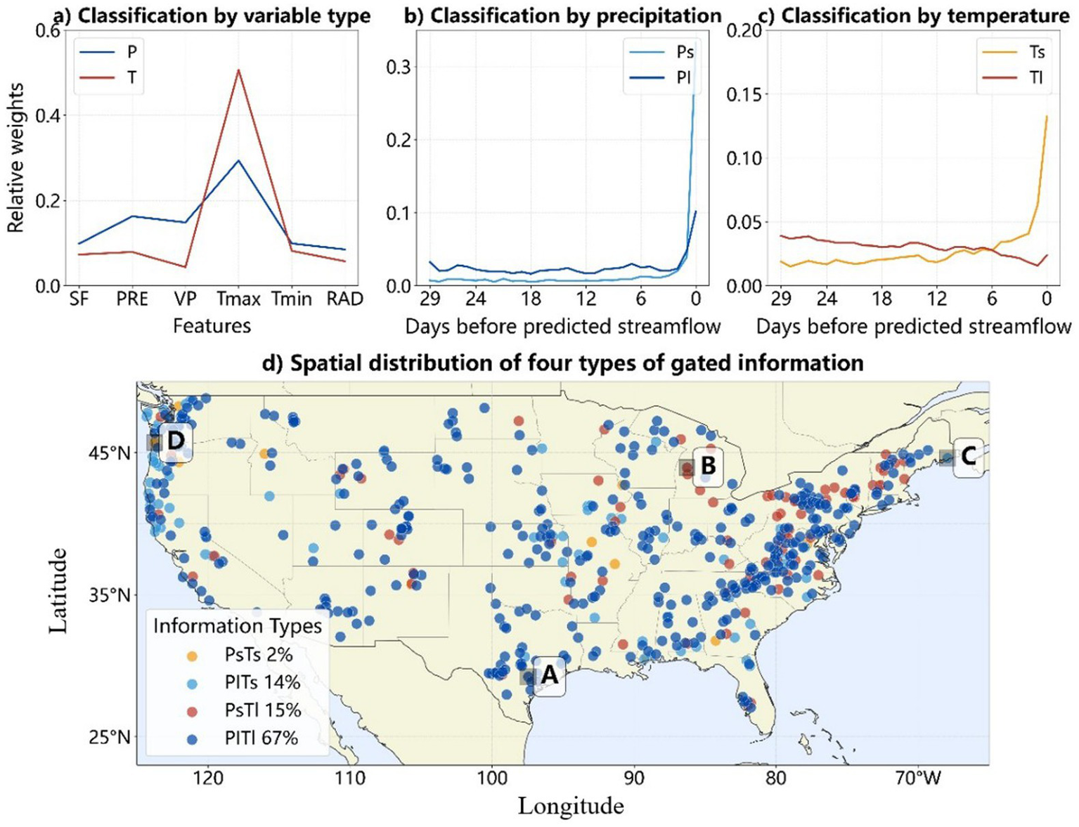
(a) The average relative weights of P-type and T-type; (b) the average relative weights of Ps type and Pl type; (c) the average relative weights of Ts type and Tl type; and (d) The spatial distributions of four types of gated information where a–d represent PlTl, PsTl, PlTs, and PsTs, respectively.
When combining the precipitation and temperature types, we obtain the mechanisms for the stations: PsTl, PsTs, PlTl, and PlTs, as shown in Figure 5d. Observations indicate that PsTl accounts for roughly two-thirds of all sites, primarily distributed in the central and eastern parts of the continent. The proportion of PsTs is only 15%, mostly concentrated in the northeastern region. This indicates that short-term precipitation is dominant, accounting for over 80%. Similar in number to PsTs, PlTl accounts for 14% and is predominantly found in the northwestern regions. The least frequent type, PlTs, makes up only 2% and is scattered across northwestern and central areas. These observations suggest that temperature tends to be long-term, while precipitation is short-term. To demonstrate the characteristics of different types of gated information and their relationship with streamflow, we select four stations (Station A-D in Figure 3d). The selections are carefully made to cover a wide range of latitudes and longitudes, thereby providing a comprehensive representation of the aggregated clustered types.
For the PsTl class, station A located in the south is selected (Figure 5d). Gated information for station A is presented in Figure 6a, which has a distinct characteristic of favoring temperature over precipitation, as evident from its higher overall temperature-to-precipitation control ratio. It can be found that recent precipitation and vapor pressure have high pass rates. However, when considering overall significance, the temperature information within nearly all time periods needs to be propagated to the subsequent model layer. Its weight distribution remains relatively consistent throughout the historical period. Temperature not only affects the evaporation rate but also influences soil moisture content. This could be a reason why the Tl type is also present in the southern region. In the corresponding time series plot (Figure 6b), the measured streamflow at station A is represented by the red line, while the streamflow predicted by the model is depicted by the blue dashed line. The highest flow level is indicated by the black pentagram. The corresponding daily precipitation, shown by the green line, exhibited a clear correlation with the peak flow. There is an inconsistency in the relationship between heavy precipitation and flood peaks. For instance, in 2005, there are two peak flood events with daily streamflow reaching approximately 6,000 m3. Despite heavy rainfall occurring on both occasions, the second rainfall is significantly heavier, exceeding 100 mm. Surprisingly, there is not much difference between the two peaks. This suggests that the flood mechanisms in these two events are different. Furthermore, the largest flood occurred in 2007, whereas precipitation is not very heavy in this flooding period. This inconsistency also indicates that precipitation is not the primary driving factor for this flood. It is possible that temperature information could play a crucial role in improving the model performance for this type of stations.
Figure 6

Visualization of gated weight heatmaps on the left columns and time series plots of streamflow on the right columns for station A (subplot a,b), station B (subplot c,d), station C (subplot e,f), and station D (subplot g,h). In the gated weight heatmaps, the variables SF, PRE, RAD, Tmax, Tmin, and VP denote streamflow, precipitation, radiation, maximum temperature, minimum temperature, and vapor pressure, respectively. In the time series plots, the streamflow measured and predicted by the LSTM model are represented by the red and blue dash lines, respectively while the corresponding daily precipitation is indicated by the green lines. The highest flow level is indicated by the black pentagram.
Station B, located in the northern region, represents the PsTs class. Its gated information displays high values for streamflow and low values for other variables (Figure 5c). Unlike the PsTl type in Figure 6a, the gated information for temperature diminishes across all 30 days without any effect. This indicates that the model does not require temperature data to make accurate predictions at this station, implying the station’s flood generation mechanism is not related to temperature. Regarding the time series plot (Figure 6d), the streamflow at this station shows distinct dry seasons and rainy periods. For the extreme flow labeled as the highest peak in 2008, there was heavy precipitation 1 or 2 days preceding the peak, aligning with the threshold criteria suggested by the gated weights, requiring consideration of short-term data. The strong correlation between precipitation and streamflow implies that brief periods of precipitation can quickly trigger rises in streamflow.
The PlTl category, exemplified by station C in the east, has a higher pass rate for long-term information for both precipitation and temperature (Figure 6e). In the gated information plot, precipitation is the variable that requires the most information after temperature. The temperature information indicates that the temperature data for the upcoming forecast days is not as important as the overall temperature performance. Additionally, temperature exhibits a clear seasonal periodicity, and there is a strong correlation between the highest and lowest temperatures. Therefore, when the information about the lowest temperature is emphasized, the information about the highest temperature can sometimes be disregarded. The streamflow at this station exhibits significant fluctuations, with a low base flow during most time periods (Figure 6f). Meanwhile, heavy precipitation events clearly increase the volume of streamflow. For instance, during the 2001 flood, a precipitation of over 100 mm results in a flow of nearly 25, 000 m3/day. Since the precipitation for the predicted day is not included in the model calculation, this non-cyclical and highly variable curve may require more days of information to predict sudden increases in runoff. Additionally, it is worth noting that heavy rainfall does not always lead to a significant rise in streamflow. For example, during 2006, despite several rainfall events exceeding 50 mm/day, the change in streamflow is not substantial. This may be attributed to that this station is located in the southern region, where the predominant streamflow generation mechanism is storage overflow. Runoff only occurs when the soil moisture content reaches its maximum capacity.
For the final class, PlTs, station D in the northwest is chosen (Figure 5d). Figure 6g presents the gated information, where the gating value for precipitation on the final day is notably higher than the rest, yet still >0 for most other days. This emphasizes the significance placed on hydrological variables like streamflow, precipitation, and vapor pressure, leading to its categorization as a P-type station. Simultaneously, temperature primarily focuses on specific days’ information, aligning with the Ts curve in Figure 5c, hence falling into the PlTs category. In the time series plot (Figure 6h), the exceptional performance of the model at this station merits attention, achieving a CC of 0.985 and NSE of 0.970. The consistent pattern observed reinforces the substantial correlation between prolonged precipitation occurrences and peak streamflow timings. Specifically, brief intense rainfall does not consistently cause an instant surge in runoff. For example, the maximum streamflow in 2004 wasn’t brought about by the strongest rainfall. This accentuates the importance of long-term precipitation for accurate forecasting at this station.
It is important to note that the gating mechanism was applied to only four representative stations, one from each major cluster, rather than across all stations within each cluster. While these selected stations were chosen as representative samples based on their flooding mechanisms, this approach introduces an element of uncertainty regarding the generalizability of the results across all stations within each cluster. The performance of the gating mechanism at other stations within the same clusters may vary due to local microclimatic conditions, data quality issues, or other site-specific factors not captured in current analysis.
3.4 Verify the effectiveness of the gated module
Figure 6a illustrates the LSTM gated information at station A when all six input variables in the 30-day lookback window are used for the prediction model. It can be observed that radiation plays a negligible role in the subsequent model calculations. To examine the effectiveness of gated information, we remove radiation from the input variables and re-train the model using the remaining five variables. The distributions of gate weights for these five input variables are similar between the model with radiation as the input variable (Figure 6a) and the model without radiation (Figure 7a). This similarity implies that the underlying physical mechanism for the same station, as derived from the gated module, remains consistent regardless of the specific variables are used as in the model inputs. Furthermore, the simulation results show that the removal of radiation from the input variables has minimal impact on the model performance when comparing Figure 6b with Figure 7b. While the MSE value is slighter larger, and the values of CC and NSE are slightly smaller for the case where radiation is not included, the differences are not significant.
Figure 7

Gated weight heatmaps and hydrological variable time series for station A: Model configurations with 5 dominant variables as input (subplots a,b), 10-day lookback window (subplots c,d), and 90-day lookback window (subplots e,f).
Since station A is classified as the PsTl type, we conduct another experiment involving a narrower lookback window for the input variables. In Figure 7c, it is evident that the gated module consistently assigns a high priority to temperature information within a 10-day lookback window, mirroring the pattern observed in the 30-day window depicted in Figure 6a. By contrast, the higher weights of other variables are primarily concentrated within the last 1–2 days (Figure 7c). Moreover, the model with the 10-day lookback window (Figure 7d) performs similarly to the model with the 30-day window (Figure 6b). The third experiment is conducted involving a 90-day lookback window for input variables. In this case, a greater amount of information is found to pass through the gated weights, including long-term precipitation information and partial radiation information (Figure 7e). However, the model performs poorer when the 90-day lookback window is used, with a decrease in the NSE value from 0.871 for the 30-day window to 0.851 for the 90-day window (Figure 7f). This indicates that additional information might introduce noise and potentially disrupt the model’s ability to focus on the more pertinent information that should be prioritized.
The fundamental concept behind gated information is to selectively choose relevant data from the input, either by discarding or emphasizing specific segments. This process effectively reduces the amount of data and therefore facilitates the training of subsequent models. Moreover, it provides a means to visualize the variables and time series that the model considers important, enabling direct adjustments and optimizations at the input level. Additionally, this approach can be used to evaluate the value of newly added variables or time series. Nevertheless, it is important to note that we are not opposed to adding more information to the network, as the model could potentially learn new features from additional variables. Our primary goal, however, is to streamline the input variables, simplifying the learning process for the model by removing redundant and complex information. It should be acknowledged that introducing white noise or irrelevant variables will inevitably lead to a decrease in the model’s accuracy. Furthermore, it is worth mentioning that the model used in this study consisted of a simple LSTM followed by two fully connected layers. Given its relatively shallow architecture, it may struggle to capture effectively large amounts of information. This could explain why the model tended to perform better with smaller scale input data. Deepening the model architecture may potentially enhance its ability to handle variable additions. In conclusion, for the model employed in this study, removing redundant long-term series information did not compromise the accuracy of the model simulation, challenging the common practice of incorporating lengthy series and numerous variables into LSTM models without empirical validation. It is recommended to utilize gated information to determine whether long-term and multiple variables are necessary as input data for models.
4 Discussion
4.1 Comparative analysis of attribution methods
Various types of explanation methods, including gradient-based approaches (e.g., Integrated Gradients, SmoothGrad), perturbation-based methods (e.g., LIME, SHAP), and attention-based techniques, had been established to understand the interpretation of models from different perspectives. These algorithms operate on the principle that the output gradient of a neural network with respect to each input unit indicates its importance, or the effect of masking an input unit on the model’s output can reveal its significance. Deng et al. (2024) have demonstrated that these algorithms can be unified in a mathematical framework, where the model’s purpose is to calculate how to allocate independent and interactive effects. In other words, explainability algorithms are formulated to quantify the influence of an input unit on the network output, either independently, without dependence on other input units (independent effect), or through interactions with other input units (interactive effect). To validate the reliability of the Gated method proposed in this study, we conducted a comparative analysis against two widely-applied interpretability methods, Saliency and Feature Ablation.
Figure 8 shows the analysis of feature importance heatmaps across three attribution methods: Saliency, Feature Ablation, and Gated with a random station. The Saliency method highlights a pronounced increase in the importance of the SF feature toward the later stages of the time series, particularly around time step 24, underscoring its critical role in capturing long-term dependencies (Figure 8a). In contrast, other features exhibit consistently low importance, with PRE and RAD showing minimal impact on model predictions. Feature Ablation corroborates the prominence of SF but offers a more granular perspective on the contributions of secondary features like Tmax and Tmin (Figure 8b). While these features remain less influential than SF, their variability suggests potential contextual relevance under specific conditions, which is less evident in the Saliency analysis. In the Gated method’s heatmap, feature importance dynamically shifts over time, reflecting condition-dependent variability (Figure 8c). Unlike Saliency and Feature Ablation, it highlights how key features like SF maintain overall importance but still fluctuate with changing conditions.
Figure 8

Visualization of feature importance heatmaps using (a) saliency, (b) feature ablation and (c) gated methods.
Figure 9a provides insight into the inter-method similarities by illustrating the Pearson correlation coefficients between these approaches. Specifically, it reveals a strong positive correlation of 0.86 between Saliency and Gated methods, indicating substantial agreement in their attribution patterns. Conversely, the correlation between Feature Ablation and Gated is markedly lower at 0.44, suggesting more distinct attribution behaviors. Figure 9b offers a comparative analysis of average feature importance scores across the aforementioned methods for atmospheric variables including SF, PRE, RAD, Tmax, Tmin, and VP. This visualization highlights that the SF variable garners significant attention across all methods, underlining its pivotal role in model predictions. However, notable differences emerge in the attribution of importance to other variables, with each method assigning varying degrees of significance to PRE, RAD, Tmax, Tmin, and VP. Such distinctions suggest that while certain features dominate universally, others exhibit method-specific relevance, thereby informing nuanced interpretations of model behavior and guiding targeted feature engineering efforts.
Figure 9

(a) The correlation between three explainable methods and (b) feature importance across different methods.
Figure 10 comprises three subplots depicting the temporal dynamics of feature importance across different attribution methods. In Figure 10a, the Saliency method illustrates a pronounced increase in feature importance toward the latter stages of the time series, suggesting that features become increasingly pivotal as the prediction horizon extends. Figure 10b presents the Feature Ablation method, which reveals relatively stable feature importance levels throughout most of the timeline, followed by a steep rise toward the final time steps. In Figure 10c, the curve for the Gated method shares a similar shape with that of the Saliency method. Both curves exhibit a series of peaks and troughs, indicating fluctuating feature importance across time steps.
Figure 10

Visualization of temporal importance for (a) saliency, (b) feature ablation and (c) gated methods.
Overall, the results of the Gated method show a high correlation with those of the Saliency method, suggesting a certain degree of reliability in their similar attribution patterns. However, there is a notable discrepancy when comparing these results to those obtained through Feature Ablation, highlighting significant differences in how each method assesses feature contributions. These observations underscore the need for further investigation into the applicability and robustness of various interpretability methods, aiming to better understand their strengths and limitations in different contexts.
4.2 Limitations and future directions
The module designed in this study integrates considerations of both gradient and data occlusion, and facilitates the visualization by extracting intermediate layer units in a concise and convenient manner. To account for interactive effects within the module, a self-attention mechanism is employed in the gate layer. This design concept aligns with the philosophy presented by Zhang et al. (2024) and Ren et al. (2021) that the methodology must be capable of elucidating the patterns of change in the model’s generalizability. However, there currently lacks a unified theoretical foundation or framework for attribution algorithms, leading to divergent interpretability results across different methods. This divergence makes it challenging to rigorously analyze and determine which attribution algorithm is reasonable and reliable beyond the illusory sense of direct perception. Moreover, most explanation algorithms for ML are designed based on experimental experiences or intuitive cognition (Bach et al., 2015; Lundberg and Lee, 2017; Sundararajan et al., 2017). The gated module in this study was also designed and proven for its practicality through empirical experiments. Its deeper theoretical underpinnings and applicability in a broader range of scenarios still require further refinement and exploration.
The current study, relying solely on single-station data, may inherently limit the model’s ability to capture spatial variability and broader regional dynamics. To address this limitation, future research should extend the analysis to multiple stations, thereby providing a deeper understanding of the model’s performance across diverse spatial scales.
5 Conclusion
In this study, we propose an explicable model built upon the LSTM framework used for flood prediction throughout 531 catchments within the contiguous United States. We developed a simplified gated module positioned between input data and the LSTM model to discern how patterns are captured within the inputs. The proposed visual and understandable gated module affords insight into how the relationship among various variables and lookback windows are learned. Gated weight outputs enable modification of the model’s input and offer perception regarding what influences changes in streamflow. Moreover, we explore disparities among four categories derived from gated information: PsTl, PsTs, PlTs, and PlTl representing whether temperature and/or precipitation belong to either the short- or long-term classes. This categorization significantly aids our comprehension of how the flood prediction model utilizes input data along with what drives functionality. Implementing gating to selectively reduce input information does not compromise accuracy but boosts prediction strength by prioritizing crucial aspects.
Moreover, the gating method exhibits a high degree of correlation with the Saliency method in terms of feature importance attribution patterns. When compared to Feature Ablation, notable differences emerge. These discrepancies illustrate the variability among different interpretability methods and underscore the importance of selecting the appropriate method based on the specific requirements of the analysis. The gating method’s capability to capture condition-dependent variability and interactive effects among features offers a deeper understanding of model behavior beyond simple input selection. By integrating gradient considerations and data occlusion techniques, facilitated by a self-attention mechanism, it provides valuable insights into how different features interact and influence predictions over time. This enhanced understanding contributes to explaining certain mechanisms driving model predictions, highlighting its utility in improving model interpretability. However, the current study, relying solely on single-station data, may inherently limit the model’s ability to capture spatial variability and broader regional dynamics. To address this limitation, future research should extend the analysis to multiple stations, thereby providing a deeper understanding of the model’s performance across diverse spatial scales.
Statements
Data availability statement
The original contributions presented in the study are included in the article/supplementary material, further inquiries can be directed to the corresponding author.
Author contributions
ZZ: Data curation, Formal analysis, Methodology, Validation, Writing – original draft, Writing – review & editing. DW: Conceptualization, Funding acquisition, Investigation, Writing – review & editing. YM: Formal analysis, Methodology, Validation, Writing – review & editing. JZ: Data curation, Validation, Visualization, Writing – review & editing. XX: Data curation, Formal analysis, Validation, Visualization, Writing – review & editing.
Funding
The author(s) declare that financial support was received for the research and/or publication of this article. This research was funded by the National Natural Science Foundation of China (Grant no. 52079151) and the 2025 High-Level Talent Cultivation Program of Zhaoqing University (Grant no. gcc202512).
Conflict of interest
The authors declare that the research was conducted in the absence of any commercial or financial relationships that could be construed as a potential conflict of interest.
Generative AI statement
The authors declare that no Gen AI was used in the creation of this manuscript.
Publisher’s note
All claims expressed in this article are solely those of the authors and do not necessarily represent those of their affiliated organizations, or those of the publisher, the editors and the reviewers. Any product that may be evaluated in this article, or claim that may be made by its manufacturer, is not guaranteed or endorsed by the publisher.
References
1
Adadi A. Berrada M. (2018). Peeking inside the black-box: a survey on explainable artificial intelligence (XAI). IEEE Access6, 52138–52160. doi: 10.1109/ACCESS.2018.2870052
2
Addor N. Nearing G. Prieto C. Newman A. J. Le Vine N. Clark M. P. (2018). A ranking of hydrological signatures based on their predictability in space. Water Resour. Res.54, 8792–8812. doi: 10.1029/2018WR022606
3
Addor N. Newman A. J. Mizukami N. Clark M. P. (2017). The CAMELS data set: catchment attributes and meteorology for large-sample studies. Hydrol. Earth Syst. Sci.21, 5293–5313. doi: 10.5194/hess-21-5293-2017
4
Alfieri L. Cohen S. Galantowicz J. Schumann G. J.-P. Trigg M. A. Zsoter E. et al . (2018). A global network for operational flood risk reduction. Environ. Sci. Pol.84, 149–158. doi: 10.1016/j.envsci.2018.03.014
5
Altay N. Narayanan A. (2022). Forecasting in humanitarian operations: literature review and research needs. Int. J. Forecast.38, 1234–1244. doi: 10.1016/j.ijforecast.2020.08.001
6
Althoff D. Bazame H. C. Nascimento J. G. (2021). Untangling hybrid hydrological models with explainable artificial intelligence. H2Open J.4, 13–28. doi: 10.2166/h2oj.2021.066
7
Arras L. Arjona-Medina J. A. Widrich M. Montavon G. Gillhofer M. Müller K.-R. et al . (2019). Explaining and interpreting LSTMs. Explainable AI Interpreting Exp. Visualizing Deep Learning11700, 211–238. doi: 10.1007/978-3-030-28954-6_11
8
Baehrens D. Fiddike T. Harmeling S. , KawanabeM., HansenK.Klaus-Robert MuellerK-R. (2009). How to Explain Individual Classification Decisions. Journal of Machine Learning Research, 11, 1803–1831. doi: 10.5555/1756006.1859912
9
Barnhart T. B. Molotch N. P. Livneh B. Harpold A. A. Knowles J. F. Schneider D. (2016). Snowmelt rate dictates streamflow. Geophysical Research Letters, 43, 8006–8016. doi: 10.1002/2016GL069690
10
Bach S. Binder A. Montavon G. Klauschen F. Müller K.-R. Samek W. (2015). On pixel-wise explanations for non-linear classifier decisions by layer-wise relevance propagation. PLoS One10:e0136744. doi: 10.1371/journal.pone.0136744
11
Beça P. Rodrigues A. C. Nunes J. P. Diogo P. Mujtaba B. (2023). Optimizing reservoir water Management in a Changing Climate. Water Resour. Manag.37, 3423–3437. doi: 10.1007/s11269-023-03508-x
12
Berghuijs W. R. Woods R. A. Hutton C. J. Sivapalan H. M. (2016). Dominant Flood Generating Mechanisms across the United States. Geophysical Research Letters, 43, 4382–4390. doi: 10.1002/2016GL068070
13
Chen G. Chen S. Li D. Chen C. (2025). A hybrid deep learning air pollution prediction approach based on neighborhood selection and spatio-temporal attention. Sci. Rep.15:3685. doi: 10.1038/s41598-025-88086-1
14
Coulibaly P. Baldwin C. K. (2005). Nonstationary hydrological time series forecasting using nonlinear dynamic methods. J. Hydrol.307, 164–174. doi: 10.1016/j.jhydrol.2004.10.008
15
Danandeh Mehr A. Kahya E. Olyaie E. (2013). Streamflow prediction using linear genetic programming in comparison with a neuro-wavelet technique. J. Hydrol.505, 240–249. doi: 10.1016/j.jhydrol.2013.10.003
16
Deng H. Zou N. Du M. Chen W. Feng G. Yang Z. (2024). Unifying fourteen post-hoc attribution methods with Taylor interactions. IEEE Transactions on Pattern Analysis and Machine Intelligence, 46, 4625–4640. doi: 10.1109/TPAMI.2024.3358410
17
Ding Y. Zhu Y. Feng J. Zhang P. Cheng Z. (2020). Interpretable spatio-temporal attention LSTM model for flood forecasting. Neurocomputing403, 348–359. doi: 10.1016/j.neucom.2020.04.110
18
Ditthakit P. Pinthong S. Salaeh N. Binnui F. Khwanchum L. Pham Q. B. (2021). Using machine learning methods for supporting GR2M model in runoff estimation in an ungauged basin. Sci. Rep.11:19955. doi: 10.1038/s41598-021-99164-5
19
Du S. Jiang S. Ren L. Yuan S. Yang X. Liu Y. et al . (2023). Control of climate and physiography on runoff response behavior through use of catchment classification and machine learning. Sci. Total Environ.899:166422. doi: 10.1016/j.scitotenv.2023.166422
20
Godsey S. E. Kirchner J. W. Tague C. L. (2014). Effects of changes in winter snowpacks on summer low flows: case studies in the Sierra Nevada, California, USA. Hydrol. Process.28, 5048–5064. doi: 10.1002/hyp.9943
21
Greff K. Srivastava R. K. Koutník J. Steunebrink B. R. Schmidhuber J. (2017). LSTM: a search space odyssey. IEEE Trans. Neur. Netw. Learning Syst.28, 2222–2232. doi: 10.1109/TNNLS.2016.2582924
22
Gupta H. V. Kling H. Yilmaz K. K. Martinez G. F. (2009). Decomposition of the mean squared error and NSE performance criteria: implications for improving hydrological modelling. J. Hydrol.377, 80–91. doi: 10.1016/j.jhydrol.2009.08.003
23
Han H. Liu Z. Barrios Barrios M. Li J. Zeng Z. Sarhan N. et al . (2024). Time series forecasting model for non-stationary series pattern extraction using deep learning and GARCH modeling. J. Cloud Comput.13:2. doi: 10.1186/s13677-023-00576-7
24
Herath H. M. V. V. Chadalawada J. Babovic V. (2021). Hydrologically informed machine learning for rainfall–runoff modelling: towards distributed modelling. Hydrol. Earth Syst. Sci.25, 4373–4401. doi: 10.5194/hess-25-4373-2021
25
Herman J. D. Reed P. M. Wagener T. (2018). Time-varying sensitivity analysis clarifies the effects of watershed model formulation on model behavior. Water Resour. Res.54, 2351–2375. doi: 10.1002/2017WR020825
26
Hochreiter S. Schmidhuber J. (1997). Long short-term memory. Neural Comput.9, 1735–1780. doi: 10.1162/neco.1997.9.8.1735
27
Hussain D. Hussain T. Khan A. A. Naqvi S. A. A. Jamil A. (2020). A deep learning approach for hydrological time-series prediction: a case study of Gilgit river basin. Earth Sci. Inf.13, 915–927. doi: 10.1007/s12145-020-00477-2
28
Kokhlikyan N. Miglani V. Martin M. Wang E. Alsallakh B. Reynolds J. (2020). Captum: a unified and generic model interpretability library for PyTorch.
29
Kratzert F. Klotz D. Brenner C. Schulz K. Herrnegger M. (2018). Rainfall–runoff modelling using long short-term memory (LSTM) networks. Hydrol. Earth Syst. Sci.22, 6005–6022. doi: 10.5194/hess-22-6005-2018
30
Kratzert F. Klotz D. Shalev G. Klambauer G. Hochreiter S. Nearing G. (2019). Towards learning universal, regional, and local hydrological behaviors via machine learning applied to large-sample datasets. Hydrol. Earth Syst. Sci.23, 5089–5110. doi: 10.5194/hess-23-5089-2019
31
Krause P. Boyle D. P. Bäse F. (2005). Comparison of different efficiency criteria for hydrological model assessment. Adv. Geosci.5, 89–97. doi: 10.5194/adgeo-5-89-2005
32
Kwon Y. Cha Y. Park Y. Lee S. (2023). Assessing the impacts of dam/weir operation on streamflow predictions using LSTM across South Korea. Sci. Rep.13:9296. doi: 10.1038/s41598-023-36439-z
33
Li T. Lan T. Zhang H. Sun J. Xu C.-Y. David Chen Y. (2024). Identifying the possible driving mechanisms in precipitation-runoff relationships with nonstationary and nonlinear theory approaches. J. Hydrol.639:131535. doi: 10.1016/j.jhydrol.2024.131535
34
Li H. Wigmosta M. S. Wu H. Huang M. Ke Y. Coleman A. M. et al . (2013). A physically based runoff routing model for land surface and earth system models. J. Hydrometeorol.14, 808–828. doi: 10.1175/JHM-D-12-015.1
35
Liu Z. Zhou P. Chen X. Guan Y. (2015). A multivariate conditional model for streamflow prediction and spatial precipitation refinement. J. Geophys. Res. Atmos.120:787. doi: 10.1002/2015JD023787
36
Livneh B. Badger A. M. (2020). Drought less predictable under declining future snowpack. Nature Climate Change, 10, 452–458. doi: 10.1038/s41558-020-0754-8
37
Lundberg S. M. Lee S.-I. (2017). A unified approach to interpreting model predictions. Proceedings of the 31st International Conference on Neural Information Processing Systems, 4768–4777. Curran Associates Inc. doi: 10.5555/3295222.3295230
38
Ma K. Feng D. Lawson K. Tsai W.-P. Liang C. Huang X. et al . (2021). Transferring hydrologic data across continents – leveraging data-rich regions to improve hydrologic prediction in data-sparse regions. Water Resour. Res.57:e2020WR028600. doi: 10.1029/2020WR028600
39
McDonnell J. J. Evaristo J. Bladon K. D. Buttle J. Creed I. F. Dymond S. F. et al . (2018). Water sustainability and watershed storage. Nat. Sust.1, 378–379. doi: 10.1038/s41893-018-0099-8
40
Mohammadi B. Safari M. J. S. Vazifehkhah S. (2022). IHACRES, GR4J and MISD-based multi conceptual-machine learning approach for rainfall-runoff modeling. Sci. Rep.12:12096. doi: 10.1038/s41598-022-16215-1
41
Newman A. J. Clark M. P. Sampson K. Wood A. Hay L. E. Bock A. et al . (2015). Development of a large-sample watershed-scale hydrometeorological data set for the contiguous USA: data set characteristics and assessment of regional variability in hydrologic model performance. Hydrol. Earth Syst. Sci.19, 209–223. doi: 10.5194/hess-19-209-2015
42
Newman A. J. Mizukami N. Clark M. P. Wood A. W. Nijssen B. Nearing G. (2017). Benchmarking of a physically based hydrologic model. J. Hydrometeorol.18, 2215–2225. doi: 10.1175/JHM-D-16-0284.1
43
Ni L. Wang D. Singh V. P. Wu J. Wang Y. Tao Y. et al . (2020). Streamflow and rainfall forecasting by two long short-term memory-based models. J. Hydrol.583:124296. doi: 10.1016/j.jhydrol.2019.124296
44
Nourani V. (2017). An emotional ANN (EANN) approach to modeling rainfall-runoff process. J. Hydrol.544, 267–277. doi: 10.1016/j.jhydrol.2016.11.033
45
Núñez J. Cortés C. B. Yáñez M. A. (2023). Explainable artificial intelligence in hydrology: interpreting black-box snowmelt-driven streamflow predictions in an arid Andean basin of north-Central Chile. Water15:3369. doi: 10.3390/w15193369
46
Pokharel S. Roy T. Admiraal D. M. (2023). Effects of mass balance, energy balance, and storage-discharge constraints on LSTM for streamflow prediction. Environ. Model. Softw.166:105730. doi: 10.1016/j.envsoft.2023.105730
47
Ren J. Li M. Chen Q. Deng H. Zhang Q. (2021). Defining and quantifying the emergence of sparse concepts in DNNs. 2023 IEEE/CVF Conference on Computer Vision and Pattern Recognition (CVPR), 20280–20289.
48
Shen C. (2018). A transdisciplinary review of deep learning research and its relevance for water resources scientists. Water Resour. Res.54, 8558–8593. doi: 10.1029/2018WR022643
49
Sundararajan M. Taly A. Yan Q. (2017). “Axiomatic attribution for deep networks,” in Proceedings of the 34th International Conference on Machine Learning, 3319–3328.
50
Tripathy K. P. Mishra A. K. (2024). Deep learning in hydrology and water resources disciplines: concepts, methods, applications, and research directions. J. Hydrol.628:130458. doi: 10.1016/j.jhydrol.2023.130458
51
Van Houdt G. Mosquera C. Nápoles G. (2020). A review on the long short-term memory model. Artif. Intell. Rev.53, 5929–5955. doi: 10.1007/s10462-020-09838-1
52
Wang Y. Liu J. Xu L. Yu F. Zhang S. (2023). Streamflow simulation with high-resolution WRF input variables based on the CNN-LSTM hybrid model and gamma test. Water15:1422. doi: 10.3390/w15071422
53
Wilbrand K. Taormina R. Ten Veldhuis M.-C. Visser M. Hrachowitz M. Nuttall J. et al . (2023). Predicting streamflow with LSTM networks using global datasets. Front. Water5:1166124. doi: 10.3389/frwa.2023.1166124
54
Yao S. Chen C. Chen Q. Zhang J. He M. (2023). Combining process-based model and machine learning to predict hydrological regimes in floodplain wetlands under climate change. J. Hydrol.626:130193. doi: 10.1016/j.jhydrol.2023.130193
55
Zhang J. Li Q. Lin L. Zhang Q. (2024). Two-phase dynamics of interactions explains the starting point of a DNN learning over-fitted features.
56
Zhang Y. Zheng H. Zhang X. (2023). Future global streamflow declines are probably more severe than previously estimated. Nat. Water1, 261–271. doi: 10.1038/s44221-023-00030-7
57
Zhu S. Luo X. Yuan X. Xu Z. (2020). An improved long short-term memory network for streamflow forecasting in the upper Yangtze River. Stoch. Env. Res. Risk A.34, 1313–1329. doi: 10.1007/s00477-020-01766-4
Summary
Keywords
LSTM, explainable AI, interpretability, gated module, catchment analysis, flood mechanisms, flood prediction
Citation
Zhang Z, Wang D, Mei Y, Zhu J and Xiao X (2025) Developing an explainable deep learning module based on the LSTM framework for flood prediction. Front. Water 7:1562842. doi: 10.3389/frwa.2025.1562842
Received
18 January 2025
Accepted
18 April 2025
Published
12 May 2025
Volume
7 - 2025
Edited by
Minxue He, California Department of Water Resources, United States
Reviewed by
Hiren Solanki, Indian Institute of Technology Gandhinagar, India
Yihan Wang, University of Oklahoma, United States
Updates
Copyright
© 2025 Zhang, Wang, Mei, Zhu and Xiao.
This is an open-access article distributed under the terms of the Creative Commons Attribution License (CC BY). The use, distribution or reproduction in other forums is permitted, provided the original author(s) and the copyright owner(s) are credited and that the original publication in this journal is cited, in accordance with accepted academic practice. No use, distribution or reproduction is permitted which does not comply with these terms.
*Correspondence: Dagang Wang, wangdag@mail.sysu.edu.cn
Disclaimer
All claims expressed in this article are solely those of the authors and do not necessarily represent those of their affiliated organizations, or those of the publisher, the editors and the reviewers. Any product that may be evaluated in this article or claim that may be made by its manufacturer is not guaranteed or endorsed by the publisher.