The significance of groundwater contributions to New Zealand rivers

Groundwater and surface water are highly interconnected systems, with the connections varying spatially, temporally and by catchment. Representing this connectivity is of key importance for future effective water management, and to address the global decline of surface water flows. Previous studies have used baseflow separation methods to quantify the groundwater contribution to surface flow volumes. However, few studies have analysed the different dynamics of deep and shallower groundwater contributions to surface water flow rates across the flow regime and attempted to quantify this changing contribution. We analysed the distribution of fast (near-surface event flow), medium (seasonal shallow groundwater discharge) and slow (deeper groundwater) pathways into surface water flows for a case study involving 58 river water quality and flow monitoring sites across New Zealand. This involved a novel application of the chemistry assisted baseflow separation method (BACH). We found that shallow and deep groundwater pathways were the most significant contributor (>80% of the daily flow rate) to river flow at most sites at the 75th flow percentile, and for many sites even at the 95th flow percentile. These findings emphasise the need to better integrate groundwater into surface water management strategies, particularly as droughts intensify, floods become more frequent and severe, and legacy nutrient input increases under changing climate and land-use.

1 Introduction

Groundwater has long been known to be a significant contributor to river flows (Beck et al., 2013). Despite this, the dynamics and disposition of surface- and ground-water interactions remain poorly understood. This knowledge gap has been linked to decreasing river flow trends globally (Scanlon et al., 2012, 2023; Seo et al., 2018a,b; Konikow and Leake, 2014; Taylor et al., 2013; Das et al., 2021; Gorelick and Zheng, 2015), as declining river flows are attributed to increased abstractions from inter-connected groundwater systems (de Graaf et al., 2019). These declining flows are impacting the chemistry and ecology of aquatic ecosystems (Rosenberry et al., 2008), the ability to assimilate nutrient and pollutant fluxes into streams and rivers (we refer to both as rivers in this paper), and the provision of drinking water (Fan et al., 2013; Bosch et al., 2017; Singh et al., 2019). A clear understanding of the importance of the groundwater contribution to surface waters is therefore critical for effective catchment management. This paper advances our understanding of the interconnections of the surface- and ground-water components in the hydrological system (Scanlon et al., 2023; Seo et al., 2018b).

Baseflow separation methods have long been used to provide a rapid assessment of groundwater contributions to stream flow. These methods conceptualise river flow hydrographs as a combination of a lumped groundwater or “baseflow” estimate and precipitation runoff or “quick flow” (Beck et al., 2013). The lumped groundwater “baseflow” component may be variously comprised of regional groundwater flow, or more shallow near river sources such as adjacent perched aquifers, bank storage, the hyporheic zone, and braid plain aquifers (Wilson et al., 2024), and interflow from the unsaturated zone (Howcroft et al., 2019). Baseflows are represented implicitly and estimated through minimising model-to-measurement misfit rather than being based on hydrogeological properties and the simulation of hydrological processes; hence they cannot simulate spatially explicit causal relationships within the upriver catchment.

The key advantage of baseflow separation methods is that they are simple to use and can be applied even where catchment data is limited. However, this simplicity comes with compromises as different baseflow separation methods adopt alternative simple conceptualisations of groundwater inflows, each of which can introduce different biases (e.g., Yang et al., 2021), as occurs with simple representations of complex systems (Doherty and Christensen, 2011), leading to Cartwright (2022) observing that estimating the groundwater inflow to streams is not straightforward.

Typically, hydrograph baseflow separation methods are based on an analytical model (Martinez and Gupta, 2010) or are defined using filtering or smoothing methods (Lott and Stewart, 2016). Digital filters are also used (Eckhardt, 2005), where precipitation runoff and groundwater contributions are estimated based on decomposing the time series, into a series of responses with different frequencies and are similar to Fourier transforms and wavelet filtering methods. Typically, these baseflow separation techniques are based on a conceptualisation of baseflow having a longer wavelength and lower amplitude variation, while quick flow is characterised by shorter wavelengths. In New Zealand, Singh et al. (2019) applied the digital filter method at a national level to separate river flow hydrographs into two components, i.e., precipitation (quick flow) and groundwater (baseflow); note that application of this method does not involve ground-truthing. Traditionally, a stream baseflow index, defined as the ratio of the baseflow volume to total flow volume over a specified time period, is used to characterise this groundwater contribution, and is estimated using baseflow separation methods. These methods are applied to a single river location at a time and are used to reflect the upriver catchment’s average hydrological process behaviour.

End-member mixing analysis (EMMA) (Adams et al., 2009; Klaus and McDonnell, 2013) is an alternative mass balance approach to baseflow separation, which makes use of additional groundwater chemistry information to identify the groundwater components of river flow, and using river chemistry data to anchor the baseflow estimation. It uses the assumption that waters flowing through specific compartments of a combined surface and subsurface watershed have unique chemical signatures (e.g., Bugaets et al., 2023). These signatures reflect the average water chemistry sources in the capture zone above the measurement point. While attractive conceptually, this method is challenged by the difficulty of adequately characterising the source water chemistry, which typically requires high resolution sampling, and is generally accompanied by considerable uncertainty (Barthold et al., 2011; Delsman et al., 2013; Woodward et al., 2017). Cartwright (2022) also notes that the long-term variability and spatial heterogeneity of groundwater inflows also severely complicate efforts to calibrate baseflow separation techniques using such chemical mass balance methods.

A variant to both EMMA and hydrograph separation methods, is the Bayesian chemistry assisted hydrograph separation method, “BACH” (Woodward and Stenger, 2018; Woodward and Stenger, 2020; Stenger et al., 2024). BACH combines a recursive digital filter (Su et al., 2016) and EMMA in a Bayesian Framework using chemical or tracer data to inform and reduce the uncertainty of the separated hydrograph components. This combination of the strengths of both EMMA and digital filter methods allows the BACH method to harness more information than either EMMA or digital filters alone, while retaining the minimal data requirements and application simplicity of recursive digital filter methods.

The BACH method relies on river flows conceptualised as the product of time varying combinations of slow, medium and fast flow paths, which are attributed to deeper groundwater, seasonal shallow groundwater discharge, and near-surface event flow, respectively. This results in BACH being able to provide insights into possible shallow and deeper groundwater contributions to low and high stream flows very quickly, using river flow and chemical concentration data. Further, while EMMA typically requires conservative chemistry analytes, BACH is freed from this requirement, because any attenuation in groundwater, the hyporheic zone or instream is implicitly included in the concentrations assigned to each flow path (Woodward et al., 2017). Similarly, depth, area, storage and other hydraulic properties relevant to flow path delineation when using distributed numerical models, are implicitly included in the flow path filter parameters when using BACH. To date, studies using BACH have focussed on identifying nutrient load pathways into surface water ways (Woodward and Stenger, 2018; Woodward and Stenger, 2020; Stenger et al., 2024; and most recently a companion paper to this study in Yang et al., 2025).

In this study we use the advantages of BACH, to present an ambitious application of the BACH method that for the first time explores and quantifies the dynamics of changing slow, medium and fast flow path contributions to rivers across a national river monitoring network. This paper describes the application of the BACH method in a nationwide study of 58 river sites across New Zealand to quantify the dynamic contributions of fast (near-surface event flow), medium (seasonal shallow groundwater discharge) and slow (deeper groundwater) pathways into surface water daily flows. The results of this analysis are discussed followed by some conclusions on the important insights the application of the method reveals. These results provide important information for the application of integrated land and water management policy by contributing to a broader understanding of the magnitude and dynamics of the combination of near-surface and groundwater flow paths to a stream flow varying over time.

2 Methodology

2.1 General

The BACH method, developed by Woodward and Stenger (2018, 2020), assumes that a river flow hydrograph can be separated into fast, medium and slow flow components, whose relative contributions can be inferred from the temporally varying observations of water chemistry. These flow components are conceptually associated with distinct chemical end members, which have typically been differentiated using two routinely measured water analytes acting as tracers (e.g., nitrogen and phosphorous).

The method as applied to date has generally assumed fast flow components represent event-response, surface or near-surface flow, medium flow components represent seasonal shallow local groundwater flow, and slow flow components represent a persistent deeper regional groundwater pathway (Figure 1). Similar conceptualisations of these flow paths has been established in other catchment studies (e.g., Hesser et al., 2010; Broda et al., 2011; O’Brien et al., 2013; Aubert et al., 2013), and we have adopted the same flow path conceptualisation in this study. Each pathway implicitly connects land to the surface water monitoring site as depicted in Figure 1, however the method is not able to identify the spatial disposition of these pathways.

Figure 1

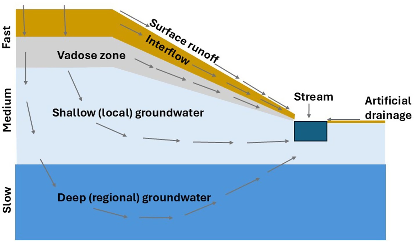
Figure 1. Schematic depiction of fast, medium and slow flow paths contributing to a river flow, modified from Stenger (2022). Surface runoff, interflow and near-surface flow contribute to fast flows into the river. Shallow groundwater provides medium flow contributions into the river. Deeper groundwater provides a slower contribution to flows.

The BACH method uses a three-component recursive digital filter (RDF) with chemical mixing models to separate the hydrograph into the fast, medium and slow flow components. Each flow component is linked to the physical near surface, shallow groundwater and deep groundwater pathways by assuming they have characteristic concentrations of each analyte, that can be considered time-invariant (Figure 2). The BACH analysis outputs comprise simulated river concentration time-series for: the mixed nutrient components that are used during history matching, the separate nutrient fluxes from the fast, medium, and slow flow components, and the fast, medium and slow contributing flows. Though not the focus of this paper, BACH outputs also include nutrient flux volumes as discussed in Yang et al. (2025).

Figure 2

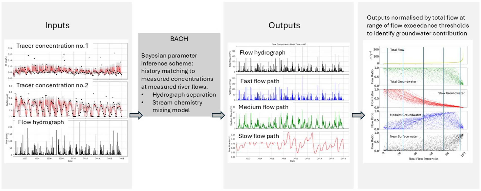
Figure 2. Illustration of BACH model inputs, their concurrent processing by the Bayesian parameter inference scheme, and resulting outputs. Modified from Stenger et al. (2024).

The BACH signal filtering method conceptually models a flow response to long term recharge and rainfall events, with the incorporation of water chemistry information. The outcome is a hydrograph separation that better reflects slow to fast rates of movement through the catchment system by inferring dominant flow path velocities.

The BACH model is described fully in Woodward and Stenger (2018, 2020), but we give a brief summary here for clarity. The method uses two RDFs, that separate the river flow ($y_n)$ on day $n$, first, into fast flow $\left(f_n\right)$ and remaining flow $\left(r_n\right)$ (Equation 1), and then into medium flow $\left(m_n\right)$ and slow flow components $\left(s_n\right)$ (Equation 2):

$\begin{array}{ll}{f}_n=y_n-r_n& (1)\end{array}$

$\begin{array}{ll}{m}_n=r_n-s_n,& (2)\end{array}$

where $r_n$ is estimated by the first RDF:

$\begin{array}{ll}{r}_n=min\left(y_{n,}\right(a_{1,m}\ast r_{n-1}+b_{0,m}\ast y_n\left)\right),& (3)\end{array}$

And the second RDF, $s_n$ is estimated by

$\begin{array}{ll}{s}_n=min\left(r_{n,}\right(a_{1,s}\ast s_{n-1}+b_{0,s}\ast r_n\left)\right).& (4)\end{array}$

Here, $a_{1,m}$, $b_{0,m}$, $a_{1,s}$, and $b_{0,s}$ are filter parameters in the interval [0,1], with the constraint that a₁/(1 − b₀) ≤ 1, this constraint is also used in Eckhardt (2005) and Su et al. (2016). These filter parameters are estimated along with component concentration parameters (for each analyte; c_f, c_m, and c_s for fast, medium, and slow component analyte concentrations, respectively). The mixing model (Equation 5) predicts analyte concentration in the river (on day n) as:

$\begin{array}{ll}{y}_n\ast c_n=f_n\ast c_f+m_n\ast c_m+s_n\ast c_s.& (5)\end{array}$

In the current study, $c_f$, $c_m$, and $c_s$ are assumed to vary nonlinearly through time according to the following harmonic form, as described in Equation 6 (Woodward and Stenger, 2020),

$\begin{array}{ll}{c}_t=e_0\ast (1-x)+e_1\ast x+f_1\ast sin\left(\mathit{\pi x}\right)+f_2\ast sin\left(2\mathit{\pi x}\right)& (6)\end{array}$

where $e_0$ is the initial concentration, $e_1$ is the final concentration, $x$ is the time scaled between 0 and 1, and $f_1$ and $f_2$ are harmonic coefficients to be inferred.

If using two analytes, as in this study where we used nitrate-nitrite nitrogen (NNN) and total phosphorus (TP), a total of 28 parameters are estimated when applying the BACH model, i.e., the four filter parameters in Equations 3, 4, and 12 concentration parameters for each analyte ($e_0$, $e_1$, $f_1$, and $f_2$ for each flow path component).

2.2 Model convergence, goodness of fit and uncertainty quantification

History matching of the model parameters was achieved using the Bayesian Markov Chain Monte Carlo (MCMC) methodology, this was implemented using the Stan algorithm (Stan Development Team, 2024). Goodness of fit metrics, as described below, are used to evaluate the credibility of the model parameterisation.

Detail on the specific computation algorithm and its implementation in BACH can be found in Woodward and Stenger (2018, 2020), and references therein. In our study, we employed the Gelman and Rubin (1992) statistic, often known as the R-hat statistic, to determine convergence of the MCMC algorithm. It is a metric for analysing the variability of samples collected from multiple chains of a Bayesian sampling method. It is defined as the sample size-adjusted ratio of between-chain variance to within-chain variance (Equation 7).

$\begin{array}{ll}R\approx \frac{\text{between}-\text{chain variance}}{\text{within}-\text{chain variance}}.& (7)\end{array}$

where between-chain variance is the variance of the parameters across all Markov chains, within-chain variance is the average of the variance in the parameters for each chain.

An R-hat near to one, suggests convergence to a stable posterior distribution. Values noticeably higher than 1 indicate that more iterations are required for improved convergence. In our study we aimed for a Gelman-Rubin statistic of 1.1, as suggested by Gelman et al. (2004).

We also used a goodness-of-fit statistic to evaluate model to measurement fit. In this investigation, we used daily flow and available coincident river NNN and TP data to calibrate our BACH models (refer to Supplementary Table S4), initially assuming that the standard uncertainty for each analyte was 0.02 mg L⁻¹ for TP and 0.2 mg L⁻¹ for NNN as employed by Woodward and Stenger (2018).

The root mean squared error (RMSE) is the most used goodness-of-fit statistic in BACH: RMSE measures the average squared difference between observed and predicted values, providing a sense of the model’s accuracy in the original units of the data to assess the goodness-of-fit of model findings and to provide a visual comparison of simulated and modelled data. A generalised form of the RMSE (GRMSE, after Woodward and Stenger, 2018) is presented below. This provides a measure of reliability of the estimated “endmember” concentrations for fast, medium and slow flows components, and the ratio of flow components from low to high flows based on how well they provide outputs that can reproduce the observed phosphorous and nitrate concentrations:

$\begin{array}{ll}\text{GRMSE}=\sqrt{\frac{1}{\mathit{nD}}\sum _{j=1}^{\mathit{nD}}2{\sigma }_{\mathit{Dj}}^2\left[l\right(0)-l({\widehat{D}}_j-D_j\left)\right]}& (8)\end{array}$

where, ${\widehat{D}}_j$ is value of the jth observation, with a total number of $n_D$; $D_j$ is the corresponding model prediction value; $l({\widehat{D}}_j-D_j)$ is the log-likelihood of residual $({\widehat{D}}_j-D_j)$, while $l\left(0\right)$ is the log-likelihood of $({\widehat{D}}_j-D_j)$ being zero; ${\sigma }_{D_j}$ is the standard deviation of the observation.

The initial 3 years of the time series are used as warm-up data, and hence goodness of fit criteria are only applied after that time.

The goodness of fit metrics do not necessarily provide a reliable indication of the uncertainty of the model predictions of fast, medium and slow flow components (Kitlasten et al., 2022). Instead, the MCMC adopted with BACH is used to quantify the uncertainty of the simulated outputs due to parameter non-uniqueness, model simplification, observation error and an assumed prior parameter distribution.

2.3 Groundwater contributions to river flow dynamics

Previous studies have used the BACH method to explore the fast, medium and slow flow path contributions to estimate nutrient loads to rivers. In this study we instead explore groundwater contributions to flow rates. Fast, medium and slow contributions to river flows can be analysed for any hydrograph, and the patterns of these pathways in river dynamics can be explored across the cumulative flow distribution. We discuss the contribution of different flow pathways to river flow rates, with pathway contributions normalised as percentages of the measured total flow at seven selected flow exceedance thresholds or “percentiles” (i.e., 1st, 5th, 25th, 50th, 75th, 95th, 99th) at each of the selected river monitoring sites.

To explore potential relationships between the BACH separated flow ratios and a representative site characteristic we utilised the flashiness index (FI) as used in Woodward and Stenger (2018) (Table 1). The FI (Equation 9) is a dimentionless measure of the river flow variability at short timescales. It is computed by dividing the pathlength of flow oscillations for that time period (i.e., the sum of the absolute values of daily variations in mean daily flow) by the total discharge for a given time period (Baker et al., 2004; Equation 8). A higher FI number implies a river in which the flow varies quickly and is often associated with reduced baseflow contributions (Deelstra and Iital, 2008).

$\begin{array}{ll}\mathrm{FI}=\frac{\sum _{i=1}^n\mid q_i-q_{i-1}\mid }{\sum _{i=1}^n{q}_i}& (9)\end{array}$

where FI is the Flashiness Index, $\sum _{i=1}^n\mid q_i-q_{i-1}\mid$ is the sum of the absolute values of daily changes in mean daily flow (pathlength of flow oscillations), $\sum _{i=1}^n{q}_i$ is the total of the mean daily flows.

Table 1

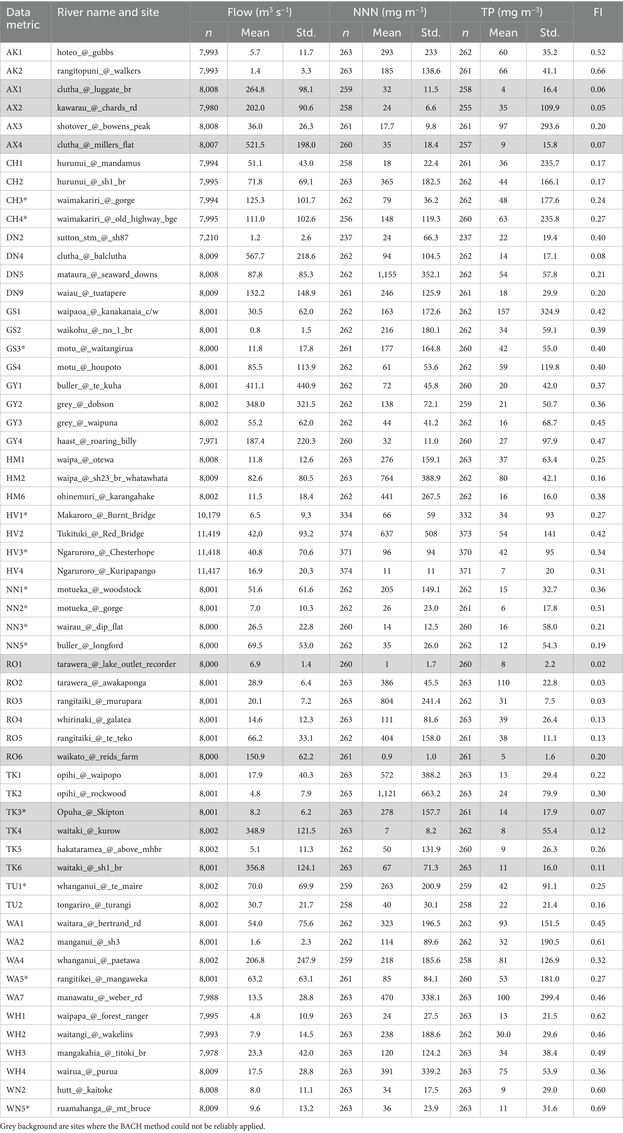
Table 1. Statistics of count, mean, and standard deviation for observed annual mean flow, TP, NNN, and FI for sites assessed in this study.

2.4 New Zealand case study

New Zealand river catchments occur across multiple geologies, soils, topographies, land uses, and rainfalls, resulting in multiple catchment types. Many of these catchments have headwaters in hilly or mountainous terrain, and outflows at the coast, and are associated with mapped alluvial aquifers. In most of these catchments groundwater flow is known to interact substantially with the surface water flow systems (Yang et al., 2025; Singh et al., 2019).

The data were supplied by the New Zealand Institute of Water and Atmospheric (NIWA) National River Water Quality Network (NRWQN, 2024; Ballantine and Davies-Colley, 2014). Surface water flow and water quality time-series data suitable for BACH analysis were available for 58 sites across our New Zealand case study (Figure 3 and Table 1). Further site details can be found in Supplementary Table S4.

Figure 3

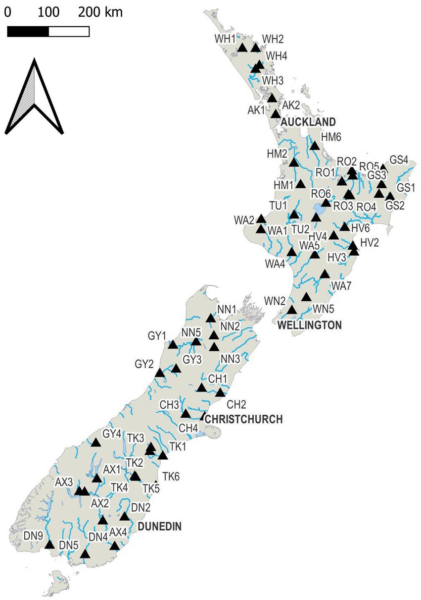
Figure 3. Location of the 58 New Zealand River Water Quality Network monitoring sites used across the New Zealand case study.

Flow time series data was available at daily intervals at all sites, but with some data gaps that were filled using linear interpolation methods. Generally, the dataset provided monthly measurements of water quality analytes, collected by a combination of automated and grab samples. The time series of flow and water quality generally spanned more than 20 years (e.g., Figure 4).

Figure 4

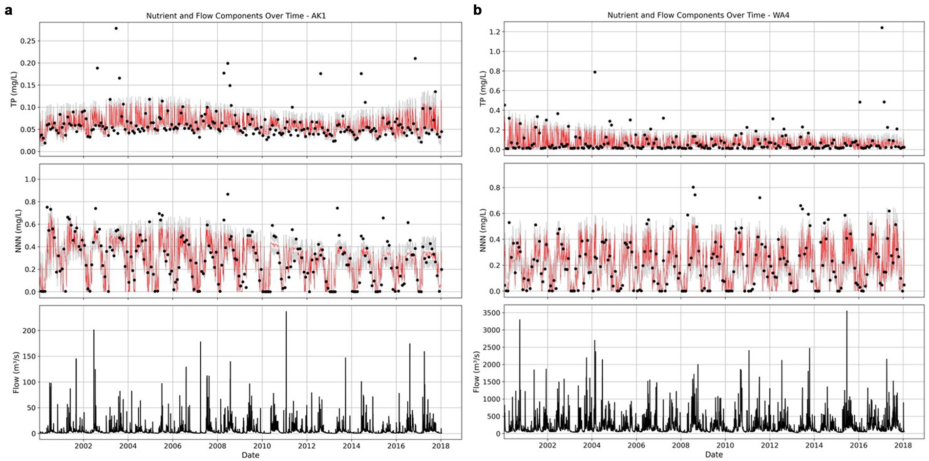
Figure 4. Simulated and observed TP and NNN concentrations and flows at site; (a) AK1 and (b) WA4. The model prediction for TP and NNN are displayed in red for the median model prediction, and grey bands include the 95% credible interval (which reflects parameter uncertainty).

We elected to use the combination of flow, TP and NNN data for the BACH analysis, as these analytes were most widely available in NRWQN (2024). Variations in the river TP and NNN concentrations at varying flow rates were used to identify distinct water quality signatures associated with slow, medium, and fast surface water flow components. This enabled us to explore the deeper and shallower groundwater pathway contributions to river flow across the full hydrograph range for multiple sites in New Zealand.

The reliability of flow-concentration relationships, and therefore the performance of the BACH method can be compromised by artificial modulation of the flow response to catchment recharge events. This includes the presence of dams, controlled flows, and lakes—the presence of these features is inconsistent with the governing assumptions of the applied methodology. The flows at monitoring site AX1 on the Clutha River, for example, are impacted by the dam on Lake Hawea (as well as by buffering from the lake itself), while flows at site AX2 on the Kawarau River are likely impacted by the buffering effect of Lake Wakatipu and the control gates that influence lake outflow, and at Clutha River site AX4 by the Roxburgh Dam. The sequence of hydroelectric dams on the Waitaki River strongly modulates flow at site TK4, as well as at the downriver, non-convergent site TK6. Sites RO6 and RO1 are proximally downriver of the outflows of Lake Taupō and Lake Tarawera, respectively, and the flow-concentration relationship is likely to be impacted by buffering of the lakes. Site TK3 on the Makaroro River, had a large number of gaps in the site flow record, and Site RO1 had very low nutrient concentration, compromising the ability to use these data time series. These eight sites were removed from the analysis (see grey shading in Table 1), leaving a total of 50 sites used for this analysis.

Observation weights assigned in the BACH analysis were initially based on the assumption of a uniform standard uncertainty across all sites (0.2 mg L⁻¹ and 0.02 mg L⁻¹ for TP and NNN, respectively), with a Gaussian distribution assumed for observation errors. These weights essentially serve as a fitting tolerance, reflecting the anticipated combined error from measurement error and model structure and parameterisation error (Woodward and Stenger, 2018). For the sites with very low concentrations, this error term was subsequently reduced, to ensure the signal was not obscured by underfitting (refer to Section 3.1).

3 Results and discussion

3.1 Data summary

A range of catchments with various dimensions, topography, hydrogeology and land use patterns are represented across the monitored sites. Summary statistics for the flow, NNN, and TP datasets used in the analysis, for each site, are presented in Table 1. Across these sites the mean flows and concentrations vary widely. For example, the mean flow across all sites ranges from a minimum of 0.8 m³ s⁻¹ (site GS2) up to 567.7 m³ s⁻¹ (site DN4), the mean NNN concentration varies from 0.9 (RO6) to 1,155 mg m⁻³ (site DN5) and the mean TP concentrations varies from 4 (site AX1) and 157 mg m⁻³ (site GS1).

At a number of sites with low nutrient concentrations, some adjustment of the observation weights was required to enhance the signal to noise ratio, and to facilitate the extraction of the flow partitioning information used by the BACH model (see Section 3.2). These sites are denoted by an “*” symbol in Table 1, if TP or NNN was a concern. Weights adjustment generally involved an iterative increase in observation weight (i.e., seeking a tighter fit to the data) for sites with low TP and NNN concentrations. However, in a few cases the weights were decreased to avoid fitting to noise. The final weights and parameters applied to the data at each site are listed in Supplementary Table S1.

3.2 History matching

History matching with the BACH model was able to establish fast, medium and slow flow components of river flow, based on acceptably good fits to the measured nutrient concentrations for all 50 sites used in the analysis. Figures 4, 5 depict the model to measurement fits to the observed instream concentration values (depicting the AK1 and WA4 sites). These 50 sites all converged to an acceptable level as defined by the Gelman R statistic, with the R-hat values all within the acceptable 1–1.1 range. The performance of the model is slightly challenged however in reproducing high observed TP concentrations, while the model was able to fit intermediate and low TP concentrations reasonably well. This reflects a weakness of the BACH model, which does not represent the non-linear increases in TP entering near-surface pathways during storm events as particulates.

Figure 5

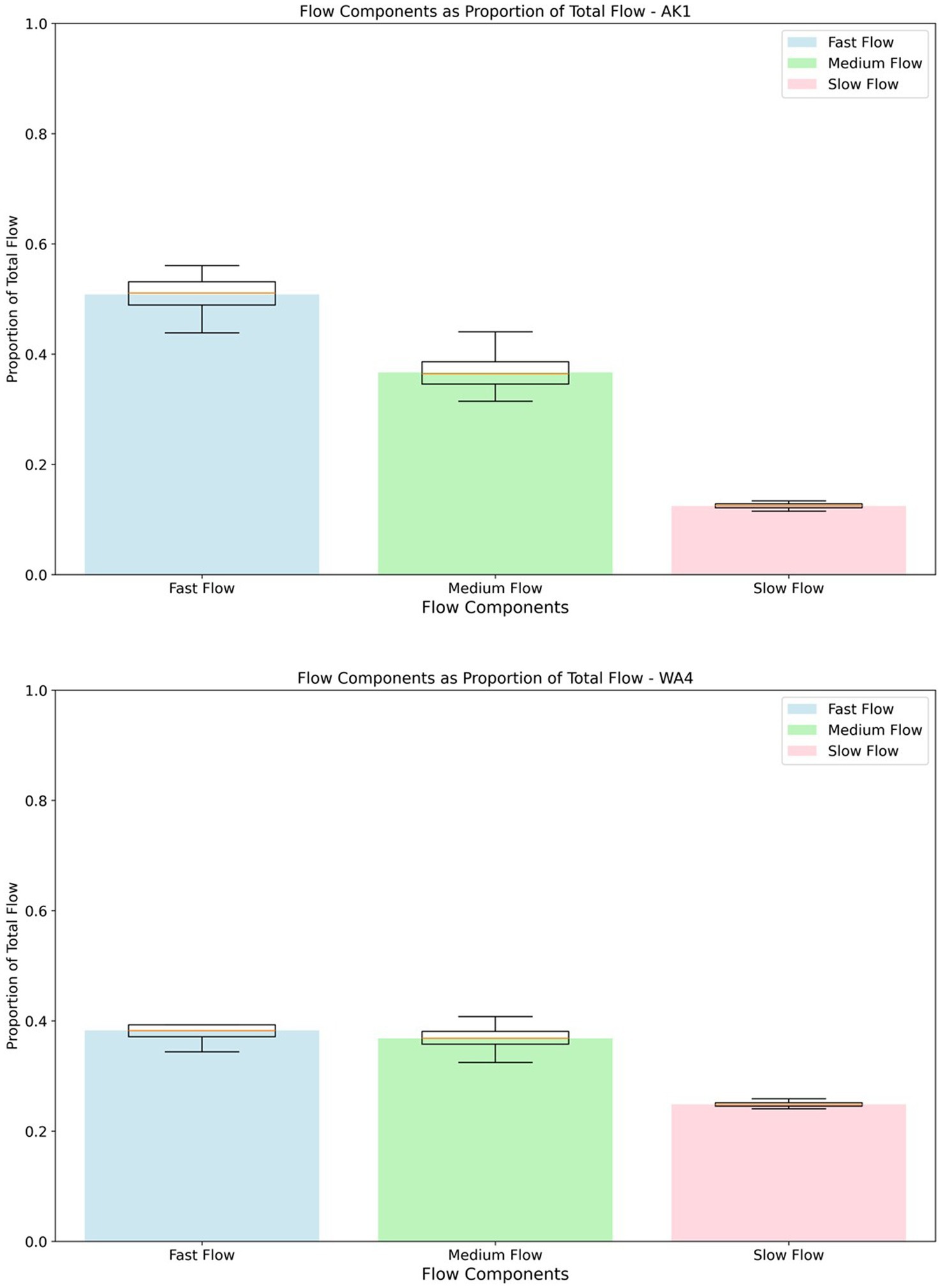
Figure 5. Predicted flow contributions as a fraction of total flow volume over the 20 year period for sites AK1 and WA4. Boxplots indicate the 0.025, 0.25, 0.5, 0.75, and 0.975 uncertainty quantiles for the inferred value.

The BACH method relies on the presence of a clear (and simple) relationship between river flow and analyte concentrations to effectively and reliably separate flow components. At the same time BACH allows the hysteresis between the flow components to be represented, allowing the mix of flow path components for any flow rate to vary on the rising and falling limb of a hydrograph. At other sites the relationship between these variables appears even more complex. Despite a converging solution, it was sometimes challenging to reproduce (relatively infrequent) high TP concentrations, suggesting that there is a stream flow and phosphorous loading behaviour that the BACH model conceptualisation is unable to represent as depicted in Figures 4, 5 for sites AK1 and WA4, with mean flows of 5.7 m³ s⁻¹ and 206.8 m³ s⁻¹, respectively. At other sites it was difficult to achieve an acceptable converged solution without careful attention to observation weights, and this reflects the lack of a unique parameter solution potentially caused by similar flow path tracer concentrations. Application of BACH at these sites is presumably challenged by the absence of strong relationship between river flow and analyte concentrations and potentially contamination of the relationships by erroneous data points.

The fits to the NNN observations in Figure 4 indicate some bias in the simulated concentration values, with high NNN concentrations biased low. Woodward and Stenger (2020) suggested that similar biased trends could be related to structural deficiency within the model inhibiting its ability to represent flashy system behaviour and its relationship to Total Nitrogen concentration.

Many sites demonstrate strong seasonal signal in NNN concentration data. For example, in the case of AK1 and WA4 (Figure 4) NNN concentrations peak in winter. Typically, where such seasonal variations are present the BACH model is able to reproduce them. However, there is still variation in the fit of the NNN predictions, with greater misfit occurring for more extreme observed values (e.g., near zero concentrations).

TP observations are not dominated by seasonal processes to the same extent. The modelled TP time series typically has greater variability, with a higher frequency and amplitude of variations, than observations. Peak observed concentrations, especially for TP, are often not well reproduced by the BACH model. These model to observation misfits can be attributed to system dynamics that are not well represented by the underlying simplifying assumptions of the BACH model.

The magnitude of the prediction uncertainty varies from site to site. Generally, for most catchments the GRMSE was around or below the assumed standard deviation for each analyte (e.g., 0.02 mg/L for TP and 0.2 mg/L for NNN, Supplementary Figure S1). The GRMSE for a number of sites is well below the assumed standard deviation (especially for NNN). This may be an indication that the model is over-fitting. However, it is noted that the sites with particularly low GRMSE generally have low concentrations, and hence a lower GRMSE is appropriate.

We note that despite some poor fits to the concentration time series, Stenger et al. (2024) observed that in general the relative pathway flow contributions had small errors. Our study is consistent with this, with all sites estimating the proportion of flow path contributions to stream flow with a small uncertainty quantified from the MCMC process (e.g., Figure 5). Slow (deep groundwater) flow path contributions typically have the narrowest confidence interval, with medium (shallow groundwater) and fast (near surface) flow contributions having slightly larger confidence intervals, indicating greater correlation between the medium and fast flow paths.

As mentioned above, field validation of chemistry assisted baseflow separation techniques using such chemical mass balance methods are challenged by long-term variability and spatial heterogeneity of groundwater inflows. However, two of the study catchments (HM6 and HV2) have relatively hydrogeologically simple catchment flow systems with some long-term groundwater nitrate concentration data (Moreau et al., 2025). We compared stream NNN concentrations for these sites with the groundwater nitrate concentrations in the surrounding catchment; we focussed only on measured nitrate concentrations, as in groundwater NNN is almost solely comprised of nitrate. Assuming a simplifying assumption of a medium and slow flow path separation depth of 80 m and 90 m below ground surface in the HM6 and HV2 stream catchments respectively, a reasonable correspondence between average groundwater measured concentrations and BACH flow-path concentration estimates was observed (refer to Supplementary Figure S2 and Supplementary Table S5).

However, this result does not verify the BACH flow-path insights. If independent groundwater chemistry data was more widely available, within delineated groundwater capture zones above the stream monitoring site, such a field validation of the chemistry end members could be possible, as noted by Cartwright (2022). However, it is worth emphasising that the strength of baseflow separation methods, including BACH, lies in the insights it provides quickly with little data. These insights can be used to guide future more detailed sampling and modelling work.

3.3 Contribution of groundwater to surface water flows

While previous studies using BACH analysis have focussed on nutrient loads entering rivers, also implicit in the BACH analyses is a characterisation of the surface- and ground-water interactions above the measurement site over time.

Figures 6a,b show the median of the posterior predicted timeseries for the flow pathway components for sites AK1 and WA4, respectively. From this figure it is clear that the variability of the slow flow component is significantly dampened relative to the total river flow, showing only low frequency signals. The medium flow component has a dampened frequency and amplitude of the total flow time series, while the fast flow component tends to have a frequency and amplitude commensurate with the total flow time series.

Figure 6

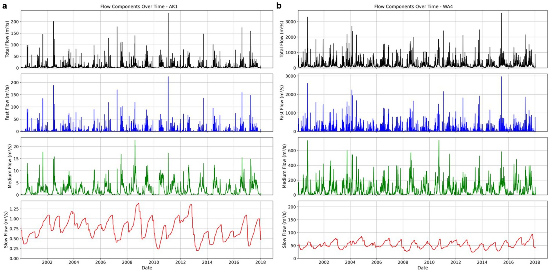
Figure 6. Separation of flow at (a) AK1 and (b) WA4 into slow, medium and fast flow components.

Also implied in Figure 6 is that groundwater input to rivers is irregular over short timescales (days to months). A similar observation was noted by Cartwright (2022), who comments that it is not clear whether baseflow as a whole varies smoothly, as is typically assumed in hydrograph baseflow separation techniques.

Due to the relative magnitude of the three flow components (e.g., slow flow, median flow and quick flow) it is often difficult to identify the changes in the dominant flow component during temporally varying river flow conditions. To address this, we explored the relative magnitude of each flow path component for the flow duration (exceedance) curve at all sites. When the three flow components are normalised by the total flow, the relative contributions of slow, medium and fast components across the flow range become more apparent. Figures 7a,b provides an example of these results for sites AK1 (Hoteo River, Auckland) and WA4 (Whanganui River) which correspond to the time series plots shown in Figure 6.

Figure 7

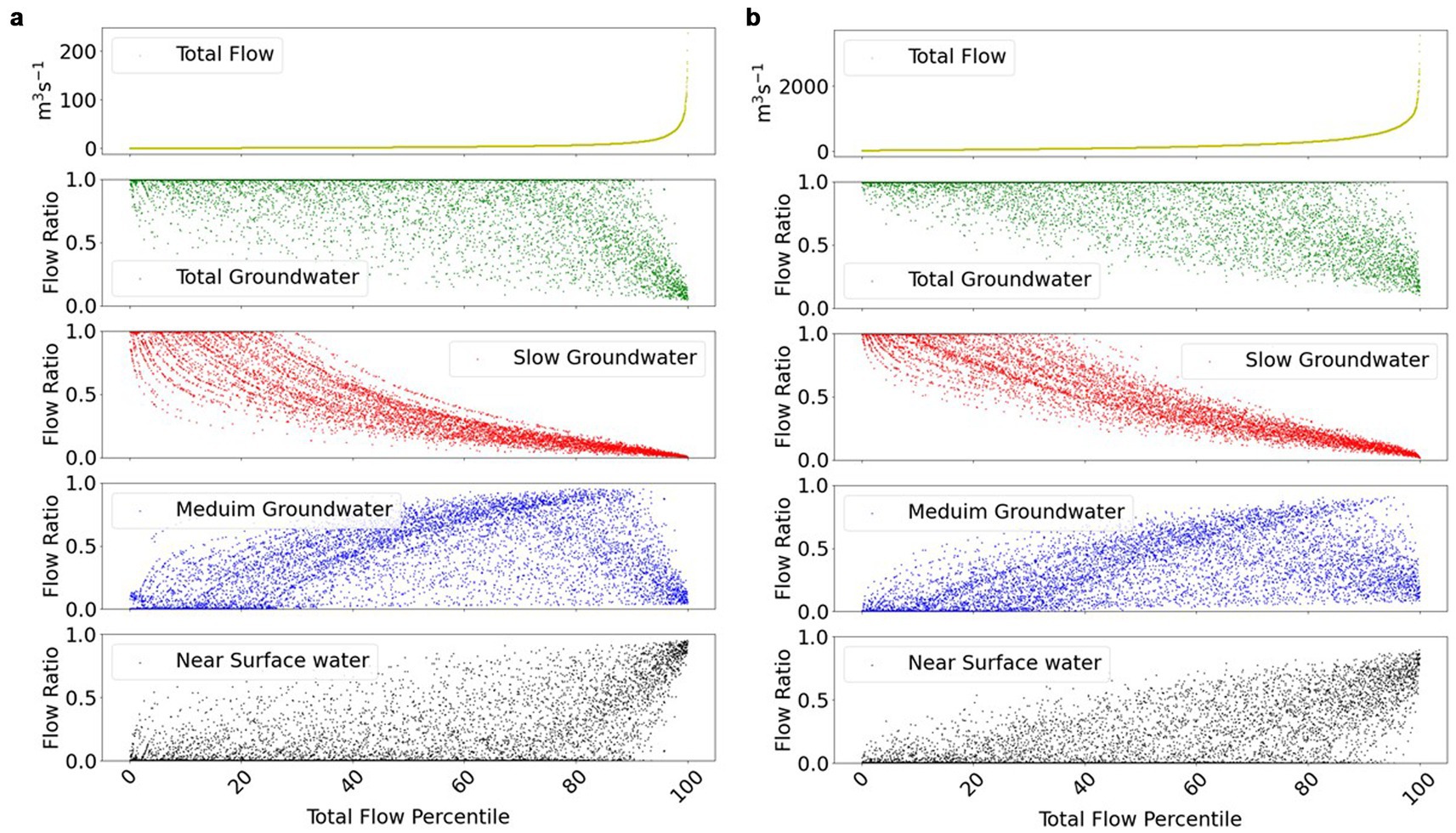
Figure 7. Flow and flow contributions summary at all flow percentiles at river sites: (a) AK1 (left), and (b) WA4 (right). Top panel is the river flow exceedance curve. Next is the ratio of total groundwater contribution to the measured river flow, then the ratio of slow (deep groundwater) contribution to measured river flow, the ratio of medium (shallow groundwater) contribution to measured river flow, and the bottom panel is the ratio of fast (near surface) flow path contribution to measured river flow.

As expected, at all sites, at low river flows (highest probability of flow exceedance) the slow flow components dominate, reflecting deeper groundwater inflow. Fast flows (reflecting near surface flows) dominate at the highest river flows. The median flow component contributions (shallow groundwater) also increase with increasing total river flow.

Different flow paths are activated during the rising limb compared to the falling limb of a flow event and seasonal patterns, with a resulting hysteresis of flow pathway characteristics (Woodward and Stenger, 2020; Bowes et al., 2005). Therefore, hysteresis in the flow path contribution to total flow ratios will depend on the antecedent or postcedent interaction between multiple dynamic components (e.g., river stage, aquifer head). Because of this the simulated flow component ratios vary for specific flow percentiles (Woodward and Stenger, 2020). The changing flow paths that are activated in the rising and falling limbs of hydrographs results in scatter or variability in these contributions for any selected river flow percentile as seen in Figure 7.

Somewhat surprising, and an important motivation for writing this paper, is the indication of the continuing importance of groundwater (both slow and medium groundwater contributions) at reasonably high flow percentiles (Figure 7). Such results suggest that high river flows are as much a function of increased medium (shallow groundwater) discharges as fast (near surface) flows. For most sites groundwater components (combined slow and medium components) dominate, even to higher flow percentiles.

We focus on flow rates as our primary interest is understanding how groundwater flow paths contribute to river flows during low flow drought events and during flood events. However, we note that previous studies using BACH have focussed on flow volumes and nutrient loads. The same flow path contributions depicted in Figure 7 could also be normalised by total volume rather than flow rate, which would tend to compress the left-hand end and expand the right-hand end of the above Figure 7.

Figure 8 shows the case study distribution of the combined groundwater flow path proportions normalised by river flow, for the 25th, 75th and 95th flow percentiles of the flow exceedance distribution for all sites. These contributions are also summarised for all sites in Supplementary Tables S2, S3. The key result in Figures 8a,b is the predominance of groundwater contributions at low flows (at the 25th flow exceedance percentile), which continues at the 75th flow percentile for most sites in this study. This groundwater contribution dominance extends to many sites even at high flows (the 95th flow percentile) as depicted in Figures 8c.

Figure 8

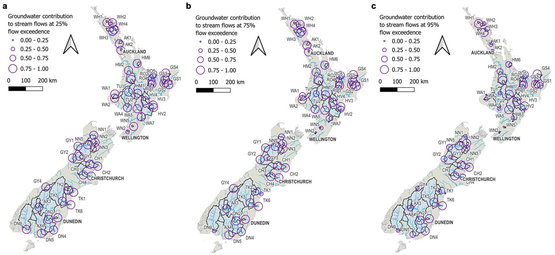
Figure 8. Contribution of groundwater components (slow and medium flow paths) to: (a) the 25%, (b) 75%, and (c) 95% river flow percentile.

These results are supported by previous work which has also indicate that groundwater plays an important contribution to river baseflows. Using a baseflow a filtering method Singh et al. (2019) found that the baseflow index indicated that on average 53% of streamflow volume in New Zealand is sustained by groundwater and other delayed sources. Similarly, Rajanayaka et al. (2020) and Ahiablame et al. (2013) found that groundwater contributed 77 and 60% of total stream volumes in the Waikato catchment (New Zealand) and sites in Indiana (USA), respectively. These studies pointed out the importance of these substantial groundwater contributions to total stream flow for adequate management of water resources and water quality.

By exploring the dynamics of the groundwater contribution to river flow, the results shown in this paper suggest that groundwater contributions to stream flow rates may be even higher, with values of groundwater contributions being commonly over 80% of river flow at the 75th flow percentile and many streams are still predominantly groundwater sourced at the 95th flow percentile.

Further, the analysis suggests that on average more than 40% of the 50th flow percentile is contributed by older water in slow flow paths. While not reflected in current water management practice, these results are consistent with those of Tetzlaff et al. (2014) who found that pre-event water (e.g., older than near surface flows) accounted for >80% of flow, even in large events. Similarly, Stewart et al. (2012), Morgenstern et al. (2010), and Stewart et al. (2010) have also identified old water contributions to river flow. The results are also consistent with Sklash and Farvolden (1979) who noted that groundwater discharge into rivers explains the temporal variations in river water chemistry which are not adequately accounted for by other theories.

Figure 9 provides a summary of the variation around the mean proportions for the 5th, 25th, 50th, 75th, and 95th percentiles for all sites. The figure shows a clear pattern of a decreasing proportion of slow flow paths and increasing proportion of medium flow paths as river flows increase at all sites. Also evident is the dominance of fast flows only at very high flows (>95% flow percentile), but with similarly high contributions also occurring from shallow groundwater flow paths. The variation in these mean flows across catchments is high and can likely be attributed to differences in surface runoff, infiltration and flashiness.

Figure 9

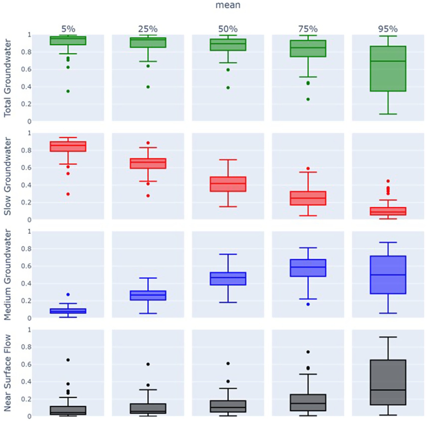
Figure 9. Box plot grid displaying median estimates of total, slow, medium groundwater, and near surface flow path contributions at 5, 25, 50, 75, and 95 river flow exceedance percentiles. Each row represents total, slow, medium groundwater, and near surface flow contributions respectively, with columns showing the distribution of these flow path contribution estimates at specified flow exceedance percentiles.

Finally, we explored the relationship between the slow flow path contributions and the FI (combining data from Table 1 and Supplementary Table S2), and found that while these are generally negatively correlated, consistent with patterns already reported in the literature (Woodward and Stenger, 2018, 2020), the correlation was not statistically significant. We note that Singh et al. (2019) and Yang et al. (2025) explored the relationship of average baseflow volumes with geological and geomorphological characteristics of catchments to extend catchment baseflow estimates and river nutrient loads to unmonitored catchments. Preliminary analyses were undertaken in this study which also indicate correlations with these characteristics, albeit with each mappable variable not correlated at a statistically significant level. Correlations of combinations of these mappable variates with the flow components would be a useful extension to this work.

4 Conclusion

Our study demonstrates two key advantages of the BACH method; (i) it can be used to provide conceptual insights on the deep and shallow groundwater contribution to stream flow very quickly and at large scales, and (ii) it can provide these insights based on only sparse datasets. This offers distinct advantages over existing chemistry assisted (e.g., EMMA) and conventional two component baseflow separation methods. These insights can then be used to guide future field programmes and modelling work.

Applying the BACH methodology to sites within the active National Water Quality Network in New Zealand provided important information on the source of river inflows. A key finding of this study, and the primary motivation for writing this paper, is the persistent and significant contribution of groundwater to river flows (both deep slow and shallow groundwater flow paths) even at high flow percentiles.

The results obtained in this study indicate that for most sites analysed, groundwater components (combined slow and medium flow components) were found to dominate flows, even at higher flow percentiles. The analyses indicate that on average more than 40% of the 50th flow percentile is contributed by slow groundwater flow paths (considered to be analogous to deeper regional groundwater flow). The combination of slow flow paths (deep groundwater) and medium flow paths (shallower groundwater) contributes more than 80% of river flows at the 75% flow percentile. For many sites this high groundwater contribution persists even at the 95% flow percentile. Meanwhile high river flows can be a function of increased medium (shallow groundwater) discharges as much as fast (near surface) flows.

Our analysis also revealed that the slow and medium baseflow components of river flows vary significantly over short time scales (days to months). This calls into question the common assumption of a smoothly varying baseflow component. Understanding these dynamics is important for a broader understanding of how the quantity and quality of baseflow may vary over time, particularly as future climate patterns change.

This study demonstrated the use of BACH, as a powerful but simple alternative to current baseflow separation methods for examining the extent and dynamics of surface- and ground-water system connectedness across the river flow regime as measured at a single location. This extends the current application of the BACH method which to date has been used to identify whether the provenance of nutrient sources in rivers originates from slow, medium or fast flow components.

A cautious approach to these results is warranted. The model is very simple, in particular the estimated magnitude of the medium flow-shallow groundwater flow pathway can be questioned, as the MCMC analysis indicates that the separation between the near surface and medium pathway is often non-unique. However, other widely used baseflow separation techniques are also simplistic, and do not have the benefit of additional information from river chemistry time series. The questioning of these previous estimates of low-moderate groundwater contributions to stream flow we consider to be the major contribution of this study. Use of water age data (Stenger et al., 2024), and groundwater chemistry concentrations to corroborate these results would be a useful extension to this study where age data becomes available.

We found that the BACH method works well wherever there is a strong relationship between flow and the TP and NNN water quality analytes, which exists in many developed catchments with intensive land use. Stenger et al. (2024) commented that other water quality analytes can be used successfully in the BACH analysis and may be more suitable in undeveloped catchments were the relationships between TP, NNN and river flows do not hold. We note that the analyses described in this paper were only applied to perennial rivers. Ephemeral rivers are estimated to be up to 51% of rivers globally (Messager et al., 2021), and it would be useful to test the performance of the BACH method in that context.

A potential extension of this study is to combine the BACH method with physically based numerical models (Ghattas and Willcox, 2021), with the goal of enhancing the efficiency and effectiveness of decision support modelling. In such an approach, the application of BACH would be to rapidly pre-process the information in hydrographs, so that only the relevant information from the time series needs to be represented in the numerical model, allowing significant run time and model complexity savings. A further benefit could be that the groundwater flow path estimation is not obfuscated by other stresses (e.g., natural stresses such as the meteorology, climate change etc.), even if they have a larger contribution to the river flow regime. In this manner the flow pathway component separation is isolated, which may provide large benefits for reducing the uncertainty in future decision-critical predictions.

Understanding these very substantial groundwater contributions to total river flow is important for any management of water resources and water quality in New Zealand and could support similar approaches in other countries. Further these results are somewhat counter to the general conceptualisation of the contributions that groundwater makes to river flows. This has important implications for management of freshwater to mitigate both drought and flood impacts, as well as for the management of river quality.

Data availability statement

Publicly available datasets were analyzed in this study. This data can be found here: https://hydrowebportal.niwa.co.nz/.

Author contributions

CM: Conceptualization, Formal analysis, Funding acquisition, Investigation, Methodology, Project administration, Supervision, Writing – original draft. PO: Conceptualization, Formal analysis, Investigation, Software, Visualization, Writing – review & editing. BH: Formal analysis, Software, Supervision, Visualization, Writing – review & editing. SC: Supervision, Writing – review & editing. JY: Conceptualization, Data curation, Writing – review & editing. MT: Data curation, Visualization, Writing – review & editing. CR: Conceptualization, Data curation, Writing – review & editing. SW: Formal analysis, Methodology, Validation, Writing – review & editing. MM: Validation, Writing – review & editing.

Funding

The author(s) declare that financial support was received for the research and/or publication of this article. This research received funding from the GNS led, New Zealand Ministry for Business, Innovation, and Employment’s Te Whakeheke o te Wai programme (Contract No. C05X1803).

Acknowledgments

The authors thank Dr. Roland Stenger of Lincoln Agritech for the constructive discussion of BACH application.

Conflict of interest

The authors declare that the research was conducted in the absence of any commercial or financial relationships that could be construed as a potential conflict of interest.

Generative AI statement

The authors declare that no Gen AI was used in the creation of this manuscript.

Publisher’s note

All claims expressed in this article are solely those of the authors and do not necessarily represent those of their affiliated organizations, or those of the publisher, the editors and the reviewers. Any product that may be evaluated in this article, or claim that may be made by its manufacturer, is not guaranteed or endorsed by the publisher.

Supplementary material

The Supplementary material for this article can be found online at: https://www.frontiersin.org/articles/10.3389/frwa.2025.1584947/full#supplementary-material

References

Adams, G. A., Cornish, P. S., Croke, B. F. W., Hart, M. R., Hughes, C. E., and Jakeman, A. J. (2009). A new look at uncertainty in end member mixing models for streamflow partitioning. Proceedings of 18th World IMACS Congress and MODSIM09 International Congress on Modelling and Simulation

Google Scholar

Ahiablame, L., Chaubey, I., Engel, B., Cherkauer, K., and Merwade, V. (2013). Estimation of annual baseflow at ungauged sites in Indiana USA. J. Hydrol. 476, 13–27. doi: 10.1016/j.jhydrol.2012.10.002

Crossref Full Text | Google Scholar

Aubert, A. H., Gascuel-Odoux, C., Gruau, G., Akkal, N., Faucheux, M., Fauvel, Y., et al. (2013). Solute transport dynamics in small, shallow groundwater-dominated agricultural catchments: insights from a high-frequency, multisolute 10 yr-long monitoring study. Hydrol. Earth Syst. Sci. 17, 1379–1391. doi: 10.5194/hess-17-1379-2013

Crossref Full Text | Google Scholar

Baker, D. B., Richards, R. P., Loftus, T. T., and Kramer, J. W. (2004). A new flashiness index: characteristics and applications to Midwestern rivers and streams. J. Am. Water Resour. Assoc. 40, 503–522. doi: 10.1111/j.1752-1688.2004.tb01046.x

Crossref Full Text | Google Scholar

Ballantine, D. J., and Davies-Colley, R. J. (2014). Water quality trends in New Zealand rivers: 1989–2009. Environ. Monit. Assess. 186, 1939–1950. doi: 10.1007/s10661-013-3508-5

PubMed Abstract | Crossref Full Text | Google Scholar

Barthold, F. K., Tyralla, C., Schneider, K., Vache, K. B., Frede, H.-G., and Breuer, L. (2011). How many tracers do we need for end member mixing analysis (EMMA)? A sensitivity analysis. Water Resour. Res. 47. doi: 10.1029/2011WR010604

Crossref Full Text | Google Scholar

Beck, H. E., Van Dijk, A. I., Miralles, D. G., De Jeu, R. A., Bruijnzeel, L., McVicar, T. R., et al. (2013). Global patterns in base flow index and recession based on streamflow observations from 3394 catchments. Water Resour. Res. 49, 7843–7863. doi: 10.1002/2013WR013918

Crossref Full Text | Google Scholar

Bosch, D. D., Arnold, J. G., Allen, P. G., Lim, K.-J., and Park, Y. S. (2017). Temporal variations in baseflow for the Little River experimental watershed in South Georgia, USA. J. Hydrol. Reg. Stud. 10, 110–121. doi: 10.1016/j.ejrh.2017.02.002

Crossref Full Text | Google Scholar

Bowes, M. J., House, W. A., Hodgkinson, R. A., and Leach, D. V. (2005). Phosphorus-discharge hysteresis during storm events along a river catchment: the River Swale, UK. Water Res. 39, 751–762. doi: 10.1016/j.watres.2004.11.027

PubMed Abstract | Crossref Full Text | Google Scholar

Broda, S., Larocque, M., Paniconi, C., and Haitjema, H. (2011). A low-dimensional hillslope-based catchment model for layered groundwater flow. Hydrol. Process. 26, 2814–2826. doi: 10.1002/hyp.8319

Crossref Full Text | Google Scholar

Bugaets, A., Gartsman, B., Gubareva, T., Lupakov, S., Kalugin, A., Shamov, V., et al. (2023). Comparing the runoff decompositions of small experimental catchments: end-member mixing analysis (EMMA) vs. hydrological modelling. Water. 15:752 doi: 10.3390/w15040752

Crossref Full Text | Google Scholar

Cartwright, I. (2022). Implications of variations in stream specific conductivity for estimating baseflow using chemical mass balance and calibrated hydrograph techniques. Hydrol. Earth Syst. Sci. 26, 183–195. doi: 10.5194/hess-26-183-2022

Crossref Full Text | Google Scholar

Das, K., Mukherjee, A., Malakar, P., Das, P., and Dey, U. (2021). Impact of global-scale hydroclimatic patterns on surface water-groundwater interactions in the climatically vulnerable Ganges river delta of the Sundarbans. Sci. Total Environ. 798:149198. doi: 10.1016/j.scitote.nv.2021.149198

PubMed Abstract | Crossref Full Text | Google Scholar

de Graaf, I. E. M., Gleeson, T., van Beek, L. P. H., Sutanudjaja, E. H., and Bierkens, M. F. P. (2019). Environmental flow limits to global groundwater pumping. Nature 574, 90–94. doi: 10.1038/s41586-019-1594-4

Crossref Full Text | Google Scholar

Deelstra, J., and Iital, A. (2008). The use of the flashiness index as a possible indicator for nutrient loss prediction in agricultural catchments. Boreal Environ. Res. 13, 209–221. Available at: http://hdl.handle.net/10138/234732

Google Scholar

Delsman, J. R., Oude Essink, G. H. P., Beven, K. J., and Stuyfzand, P. J. (2013). Uncertainty estimation of end-member mixing using generalized likelihood uncertainty estimation (GLUE), applied in a lowland catchment. Water Resour. Res. 49, 4792–4806. doi: 10.1002/wrcr.20341

Crossref Full Text | Google Scholar

Doherty, J., and Christensen, S. (2011). Use of paired simple and complex models to reduce predictive bias and quantify uncertainty. Water Resour. Res. 47:W12534. doi: 10.1029/2011WR010763

Crossref Full Text | Google Scholar

Eckhardt, K. (2005). How to construct recursive digital filters for baseflow separation. Hydrol. Process. 19, 507–515. doi: 10.1002/hyp.5675

Crossref Full Text | Google Scholar

Fan, Y., Chen, Y., Liu, Y., and Li, W. (2013). Variation of baseflows in the headstreams of the Tarim River Basin during 1960–2007. J. Hydrol. 487, 98–108. doi: 10.1016/j.jhydrol.2013.02.037

Crossref Full Text | Google Scholar

Gelman, A., Carlin, J. B., Stern, H. S., and Rubin, D. B. (2004). Bayesian data analysis: texts in statistical science series. 2nd Edn. Boca Raton, FL: CRC Press.

Google Scholar

Gelman, A., and Rubin, D. B. (1992). Inference from iterative simulation using multiple sequences. Stat. Sci. 7, 457–472. doi: 10.1214/ss/1177011136

Crossref Full Text | Google Scholar

Ghattas, O., and Willcox, K. (2021). Learning physics-based models from data: perspectives from inverse problems and model reduction. Acta Numerica 30, 445–554. doi: 10.1017/S0962492921000064

PubMed Abstract | Crossref Full Text | Google Scholar

Gorelick, S. M., and Zheng, C. (2015). Global change and the groundwater management challenge. Water Resour. Res. 51, 3031–3051. doi: 10.1002/2014WR016825

Crossref Full Text | Google Scholar

Hesser, F. B., Franko, U., and Rode, M. (2010). Spatially distributed lateral nitrate transport at the catchment scale. J. Environ. Qual. 39, 193–203. doi: 10.2134/jeq2009.0031

PubMed Abstract | Crossref Full Text | Google Scholar

Howcroft, W., Cartwright, I., and Cendón, D. I. (2019). Residence times of bank storage and return flows and the influence on river water chemistry in the upper Barwon River, Australia. Appl. Geochem. 101, 31–41. doi: 10.1016/j.apgeochem.2018.12.026

Crossref Full Text | Google Scholar

Kitlasten, W., Moore, C. R., and Hemmings, B. (2022). Model structure and ensemble size: implications for predictions of groundwater age. Front. Earth Sci. 10:972305. doi: 10.3389/feart.2022.972305

Crossref Full Text | Google Scholar

Klaus, J., and McDonnell, J. J. (2013). Hydrograph separation using stable isotopes: review and evaluation. J. Hydrol. 505, 47–64. doi: 10.1016/j.jhydrol.2013.09.0006

Crossref Full Text | Google Scholar

Konikow, L. F., and Leake, S. A. (2014). Depletion and capture: revisiting “the source of water derived from wells”. Groundwater 52, 100–111. doi: 10.1111/gwat.12204

PubMed Abstract | Crossref Full Text | Google Scholar

Lott, D. A., and Stewart, M. T. (2016). Base flow separation: a comparison of analytical and mass balance methods. J. Hydrol. 535, 525–533. doi: 10.1016/j.jhydrol.2016.01.063

Crossref Full Text | Google Scholar

Martinez, G. F., and Gupta, H. V. (2010). Toward improved identification of hydrological models: a diagnostic evaluation of the “abcd” monthly water balance model for the conterminous United States. Water Resour. Res. 46. doi: 10.1029/2009WR008294

Crossref Full Text | Google Scholar

Messager, M. L., Lehner, B., Cockburn, C., Lamouroux, N., Pella, H., Snelder, T., et al. (2021). Global prevalence of non-perennial rivers and streams. Nature 594, 391–397. doi: 10.1038/s41586-021-03565-5

Crossref Full Text | Google Scholar

Moreau, M., Herpe, M., and Santamaria Cerrutti, M. E. (2025). “2024 update of the national groundwater quality indicator” in GNS Science Consultancy Report 2024/90 (Wairakei: GNS Science), 83.

Google Scholar

Morgenstern, U., Stewart, M. K., and Stenger, R. (2010). Dating of streamwater using tritium in a post nuclear bomb pulse world: continuous variation of mean transit time with streamflow. Hydrol. Earth Syst. Sci. 14, 2289–2301. doi: 10.5194/hess-14-2289-2010

Crossref Full Text | Google Scholar

NRWQN. (2024). Available online at: https://niwa.co.nz/freshwater/water-quality-monitoring-and-advice/national-river-water-quality-network-nrwqn

Google Scholar

O’Brien, R. J., Misstear, B. D., Gill, L. W., Deakin, J. L., and Flynn, R. (2013). Developing an integrated hydrograph separation and lumped modelling approach to quantifying hydrological pathways in Irish river catchments. J. Hydrol. 486, 259–270. doi: 10.1016/j.jhydrol.2013.01.034

PubMed Abstract | Crossref Full Text | Google Scholar

Rajanayaka, C., Weir, J., Barkle, G., Griffiths, G., and Hadfield, J. (2020). Assessing changes in nitrogen contamination in groundwater using water aging: Waikato River, New Zealand. J. Contam. Hydrol. 234:103686. doi: 10.1016/j.jconhyd.2020.103686

PubMed Abstract | Crossref Full Text | Google Scholar

Rosenberry, D. O., LaBaugh, J. W., and Hunt, R. J. (2008). “Use of monitoring wells, portable piezometers, and seepage meters to quantify flow between surface water and ground water” in Field techniques for estimating water fluxes between surface water and ground water (Scotts Valley, CA: CreateSpace), 39–70.

Google Scholar

Scanlon, B. R., Fakhreddine, S., Rateb, A., de Graaf, I., Famiglietti, J., Gleeson, T., et al. (2023). Global water resources and the role of groundwater in a resilient water future. Nat. Rev. Earth Environ. 4, 87–101. doi: 10.1038/s43017-022-00378-6

Crossref Full Text | Google Scholar

Scanlon, B. R., Faunt, C. C., Longuevergne, L., Reedy, R. C., Alley, W. M., McGuire, V. L., et al. (2012). Groundwater depletion and sustainability of irrigation in the US High Plains and Central Valley. Proc. Natl. Acad. Sci. U.S.A. 109, 9320–9325. doi: 10.1073/pnas.1200311109

Crossref Full Text | Google Scholar

Seo, S. B., Mahinthakumar, G., Sankarasubramanian, A., and Kumar, M. (2018a). Conjunctive management of surface water and groundwater resources under drought conditions using a fully coupled hydrological model. J. Water Resour. Plan. Manag. 144:04018060. doi: 10.1061/(ASCE)WR.1943-5452.0000978

Crossref Full Text | Google Scholar

Seo, S. B., Mahinthakumar, G., Sankarasubramanian, A., and Kumar, M. (2018b). Assessing the restoration time of surface water and groundwater systems under groundwater pumping. Stoch. Environ. Res. Risk Assess. 32, 2741–2759. doi: 10.1007/s00477-018-1570-9

Crossref Full Text | Google Scholar

Singh, S. K., Pahlow, M., Booker, D. J., Shankar, U., and Chamorro, A. (2019). Towards baseflow index characterisation at national scale in New Zealand. J. Hydrol. 568, 646–657. doi: 10.1016/j.jhydrol.2018.11.025

Crossref Full Text | Google Scholar

Sklash, M. G., and Farvolden, R. N. (1979). The role of groundwater in storm runoff. J. Hydrol. 43, 45–65. doi: 10.1016/S0167-5648(09)70009-7

Crossref Full Text | Google Scholar

Stan Development Team (2024). RStan: the R interface to Stan T Stan Development - R package version 2.17. 3 Available online at: https://mc-stan.org/ (Accessed 2024).

Google Scholar

Stenger, R. (2022). “Nitrogen lag review” in Report 1058-14-R1 prepared for Waikato Regional Council (Lincoln: Lincoln Agritech Ltd.).

Google Scholar

Stenger, R., Park, J., and Clague, J. (2024). Routine stream monitoring data enables the unravelling of hydrological pathways and transfers of agricultural contaminants through catchments. Sci. Total Environ. 912:169370. doi: 10.1016/j.scitotenv.2023.169370

PubMed Abstract | Crossref Full Text | Google Scholar

Stewart, M. K., Morgenstern, U., and McDonnell, J. J. (2010). Truncation of stream residence time: how the use of stable isotopes has skewed our concept of streamwater age and origin. Hydrol. Process. 24, 1646–1659. doi: 10.1002/hyp.7576

Crossref Full Text | Google Scholar

Stewart, M. K., Morgenstern, U., Mcdonnell, J. J., and Pfister, L. (2012). The ‘hidden streamflow’ challenge in catchment hydrology: a call to action for stream water transit time analysis. Hydrol. Process. 26, 2061–2066. doi: 10.1002/hyp.9262

Crossref Full Text | Google Scholar

Su, C.-H., Costelloe, J. F., Peterson, T. J., and Western, A. W. (2016). On the structural limitations of recursive digital filters for base flow estimation. Water Resour. Res. 52, 4745–4764. doi: 10.1002/2015WR018067

Crossref Full Text | Google Scholar

Taylor, R. G., Scanlon, B., Döll, P., Rodell, M., van Beek, R., Wada, Y., et al. (2013). Ground water and climate change. Nat. Clim. Change 3, 322–329. doi: 10.1038/nclimate1744

Crossref Full Text | Google Scholar

Tetzlaff, D., Birkel, C., Dick, J., Geris, J., and Soulsby, C. (2014). Storage dynamics in hydropedological units control hillslope connectivity, runoff generation, and the evolution of catchment transit time distributions. Water Resour. Res. 50, 969–985. doi: 10.1002/2013WR014147

PubMed Abstract | Crossref Full Text | Google Scholar

Wilson, S. R., Hoyle, J., Measures, R., Di Ciacca, A., Morgan, L. K., Banks, E. W., et al. (2024). Conceptualising surface water–groundwater exchange in braided river systems. Hydrol. Earth Syst. Sci. 28, 2721–2743. doi: 10.5194/hess-28-2721-2024

Crossref Full Text | Google Scholar

Woodward, S. J., and Stenger, R. (2018). Bayesian chemistry-assisted hydrograph separation (BACH) and nutrient load partitioning from monthly stream phosphorus and nitrogen concentrations. Stoch. Environ. Res. Risk Assess. 32, 3475–3501. doi: 10.1007/s00477-018-1612-3

Crossref Full Text | Google Scholar

Woodward, S. J., and Stenger, R. (2020). Extension of Bayesian chemistry-assisted hydrograph separation to reveal water quality trends (BACH2). Stoch. Environ. Res. Risk Assess. 34, 2053–2069. doi: 10.1007/s00477-020-01860-7

Crossref Full Text | Google Scholar

Woodward, S. J., Wöhling, T., Rode, M., and Stenger, R. (2017). Predicting nitrate discharge dynamics in mesoscale catchments using the lumped StreamGEM model and Bayesian parameter inference. J. Hydrol. 552, 684–703. doi: 10.1016/j.jhydrol.2017.07.021

Crossref Full Text | Google Scholar

Yang, J., Moore, C. R., Rajanayaka, C., Shiona, H., Hemmings, B., Oluwunmi, P., et al. (2025). National nutrient contribution dynamics in New Zealand rivers. Hydrol. Process. 39:e70161. doi: 10.1002/hyp.70161

Crossref Full Text | Google Scholar

Yang, W., Xiao, C., Zhang, Z., and Liang, X. (2021). Can the two-parameter recursive digital filter baseflow separation method really be calibrated by the conductivity mass balance method? Hydrol. Earth Syst. Sci. 25, 1747–1760. doi: 10.5194/hess-25-1747-2021

Crossref Full Text | Google Scholar