Research on mobile ultrasonic stratified flow velocity measurement based on machine learning algorithms

A mobile ultrasonic stratified flow velocity measurement device, which utilizes a pair of ultrasonic transducers, was characterized by its low power consumption and the ability to measure multi-layer flow velocities in channels, offering advantages in water measurement applications in agricultural irrigation areas. The study combined experimental research with computational modeling to investigate the impact of ultrasonic propagation time in downstream and upstream flows and the effect of measurement position on flow velocity prediction. Traditional time-difference methods were found to be less effective for calculating water flow velocities using the proposed mobile ultrasonic transducers. By employing the AdaBoost algorithm with decision tree algorithms as weak classifiers, the relative error of the testing set was <5% in 85.71% of cases, achieving an R² value of 0.951, an RMSE value of 0.071, an MSE value of 0.795, and an MAE value of 0.654. The experimental results demonstrated that the use of the AdaBoost algorithm from machine learning for the mobile ultrasonic stratified flow velocity measurement device was feasible and effective.

1 Introduction

Research Significance Flow measurement is an indispensable technical foundation in industrial production and holds significant importance in the national economy, national defense construction, and scientific research (Ling, 2007; Sun et al., 2018). Currently, water conveyance in agricultural irrigation districts primarily relies on pipeline and open channel methods, each with different water measurement techniques. Compared to open channel methods, pipeline water measurement has relatively higher accuracy and technological maturity (Sun and Zhao, 2012). Traditional open channel water measurement methods include hydraulic structures, special facilities (flumes and weirs), and instrument-based methods. Due to the complex construction site environment, the accuracy of open channel water measurement is relatively low compared to that of pipeline measurement. According to relevant water conservancy regulations, regardless of the water measurement method used, calibration must be conducted using a rotor current meter (Rongxiang et al., 2018). This study proposes a new water measurement device—a mobile ultrasonic layered water measurement device—which consists of four parts: a stepper motor, ultrasonic transducers, a sliding rail column, and a synchronous current meter system, as shown in Figure 1. A pair of ultrasonic transducers are positioned at the same horizontal level, fixed at the bottom by two stainless steel plates, which are also attached to the shaft of the stepper motor. The middle of the stainless steel plates are welded with a horizontal support beam, which are fixed in position with the column and moves synchronously. Five current meter mounting slots were evenly distributed on this horizontal support beam for installing and calibrating current meters. Regarding research progress, traditional ultrasonic water measurement equipment is comprised of fixed single-channel and multi-channel ultrasonic current meters (Jackson et al., 1989; Jianfei et al., 2023). The former only measures the single-layer line velocity of the flow profile and does not account for the different velocity distributions in the measured flow field, leading to larger measurement errors (Zhang et al., 2019; Lee et al., 2021), particularly when flow variations are significant, which results in decreased measurement accuracy. The latter obtains corresponding local flow field information from different channels but increases equipment costs and power consumption. The increased current also introduces noise to the ultrasonic signal, causing measurement errors in multi-channel flow velocity (Xucun et al., 2023; Longhui, 2016). The mobile ultrasonic stratified flow velocity measurement device is utilized with fewer ultrasonic transducers and lower current, which does not interfere with the ultrasonic signal, thereby offering the advantage of low-power measurement of flow velocity at various water depths (Huang et al., 2024). Additionally, the device is characterized by a simple structure, making it applicable to rectangular channels of various sizes. Due to its vertical movement in the water flow, the traditional time-difference method for ultrasonic calculation is associated with relatively larger errors, which presents a pressing issue for the measurement of flow velocity and the application of the mobile ultrasonic layered water measurement device in agricultural irrigation channels.

Figure 1

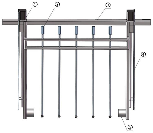
Figure 1. Schematic diagram of the mobile ultrasonic stratified water measurement device. ① stepper motors, ② rotor flow meter, ③ horizontal support beam, ④ slide columns, ⑤ ultrasonic transducers.

Accurately predicting flow velocity has significant research implications in the application of ultrasonic flow meters. Comprehensive and in-depth studies on the calculation methods for gas and fluid velocities are conducted by scholars both domestically and internationally through experimental research, theoretical analysis, and numerical simulation. Based on the principles of numerical computation methods (Ling and Fusheng, 2005; Tongfu et al., 2013), the integration of flow in circular pipes (Chapa and Rao, 2001; Wang et al., 2023) using a fixed multi-channel approach is challenging due to the volume constraints of ultrasonic transducers, making it difficult to obtain average velocities from multiple channels (Yuezhong, 2010; Pereira et al., 2022). Instead, an approximate value is derived through mathematical transformations, making measurement accuracy difficult to control (Chen et al., 2020). The velocity distribution function in the flow field was obtained by Voser (1999) through discrete numerical integration, and the weight coefficients for the Gauss-Jacobi formula were calculated. This method provided good predictive results in ideal symmetrical flows but deviated from actual flow fields (Voser, 1999). Iooss et al. (2002) described a numerical procedure to estimate the uncertainties due to these approximations in the case of fully developed turbulence. The ultrasonic propagation is modeled in 2D, moving inhomogeneous media via a ray tracing algorithm. Influence of mean profiles of temperature and velocity is studied on simple examples. Fluid temperature fluctuations and fluid velocity turbulence are considered in the stochastic framework to obtain average uncertainties on the measurements of the liquid flow rate (Iooss et al., 2002). Pannell et al. (1990) divided the circular pipe into core turbulent regions, transition regions, and laminar regions based on fluid mechanics theory. This method provides higher measurement accuracy at low Reynolds numbers but is less suitable for measuring flow in rectangular channels in agricultural irrigation areas (Pannell et al., 1990). Zheng et al. (2015) suggested first obtaining the cross-sectional distribution of the flow field using CFD simulation software and then applying Gaussian methods to correct and calculate the flow velocity, which can reduce errors to some extent. Luntta and Halttunen (1999) proposed that support vector machines, combined with particle swarm optimization algorithms, were used to determine relaxation factors and regularization parameters. This approach further established the optimal hyperplane and facilitated prediction using Lagrange multipliers and duality theory algorithms. Although this method produced good prediction results, it was noted for its low computational efficiency. Further research was deemed necessary to measure real-time flow velocity. The traditional flow calculation method based on Gaussian integration encountered numerous issues in multi-channel ultrasonic flow measurement. Zhao et al. (2014) highlighted that the two primary factors affecting the sensitivity of multi-channel ultrasonic flow measurement to the cross-sectional profile of the flow field were channel positions and weights. For the first time, a neural network computation model was applied in ultrasonic flow velocity measurement research. This significantly improved prediction accuracy by interpolating the flow field profile and applying weighted corrections to multi-channel ultrasonic flow velocities. However, the alternating backward gradient propagation of neural networks resulted in slow convergence speed, consuming significant power during computation (Jie et al., 2024; Bahrami et al., 2024). Xiaoyu et al. (2017) employed computational fluid dynamics methods based on the ultrasonic transit time method to investigate six-channel three-planar multi-channel flow measurements. It was found that when the flow field distribution was asymmetric, changes in the installation angles of multi-channel flow meters affected the flow measurement results, posing high requirements for construction sites in practical applications and making it difficult to achieve ideal results (Xiaoyu et al., 2017). Afaridegan and Amanian (2025) have demonstrated that the LSTM-ALO model, as a hybrid machine learning approach, shows significant advantages in prediction accuracy, especially in handling complex time series data in hydraulic engineering. However, the model has also faced challenges such as poor interpretability, the risk of overfitting, and high computational resource demands. In practical applications, these advantages and disadvantages need to be balanced, with corresponding optimizations and improvements considered (Afaridegan and Amanian, 2025). Adnan et al. (2025) have demonstrated that the RVFL-EROA model has proven to be an effective tool for streamflow prediction, demonstrating significant improvements in accuracy and performance, especially in regions with limited data. Its ability to handle complex relationships and estimate peak streamflow values has positioned it as a valuable asset in hydrological forecasting. However, its computational complexity and sensitivity to input choices have highlighted the need for further optimization and simplification to ensure broader applicability, particularly in real-time and resource-constrained environments (Adnan et al., 2025).

Research on multi-channel ultrasonic water measurement was focused on the ultrasonic transit time method and Doppler method for calculating flow velocity in the past. The volumetric flow rate was obtained by multiplying the line-average velocities at multiple fixed positions by corresponding weight coefficients and summing them up. This method was based on the assumption of ideal flow fields and encountered many challenges when applied in practical ultrasonic flow meters (Zhen et al., 2013). Research on mobile multi-layer ultrasonic flow measurement devices has not been reported yet. The key problem to be addressed was to draw on previous studies related to the installation angles of ultrasonic transducers (Guolong et al., 2022), while factors such as the large variation in water volume within channels in agricultural irrigation areas were considered. Through a combination of experimental research and computational model prediction, experimental studies on mobile multi-layer ultrasonic flow velocity measurement were conducted. The outcomes could provide a theoretical basis for the application and promotion of mobile multi-layer ultrasonic flow measurement devices in agricultural irrigation areas.

2 Methodology

2.1 Test configuration and procedure

The experiment was conducted in the hydraulics laboratory of the Xinjiang Water Conservancy and Hydroelectric Power Research Institute. The layout of the experimental setup is shown in Figure 2. Water from the underground reservoir was pumped to a high-level water tank and then introduced into a stilling basin. Following the stilling basin, a rectangular open channel was installed, which was 25 m long, 1 m wide, and 1.3 m deep, with a longitudinal slope ratio of 1/1,000. The open channel was constructed using brick and concrete materials, and the cement mortar was smoothed with trowels to ensure a smooth surface and tight joints with the edges of the bricks. A mobile ultrasonic stratified water measurement device was installed 10 m from the inlet of the open channel, and a control gate was placed at the end of the open channel to regulate the water depth. Downstream of the control gate, a triangular weir was installed to calibrate the flow rate in the open channel. After passing through the triangular weir, the water flowed into a return corridor and was diverted back to the underground reservoir, thus achieving a closed-loop water circulation system. In this experiment, the vertical position of the ultrasonic transducer was set as the starting point, 8 cm above the channel bottom. The distance between the ultrasonic transducer and the initial position was defined as Y_i, and the non-dimensionalization was performed by dividing Y_i by the maximum displacement Y_max, i.e., Y = Y_i/Y_max. The cross-sectional dimensions and bottom slopes of the open channels in agricultural irrigation areas vary. This experiment primarily focused on 11 different flow rates, each tested for 2 h, with specific conditions detailed in Table 1.

Figure 2

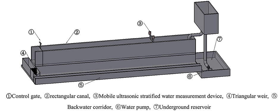
Figure 2. Layout of test device. ① Control gate, ② rectangular canal, ③ mobile ultrasonic stratified water measurement device, ④ triangular weir, ⑤ backwater corridor, ⑥ water pump, ⑦ underground reservoir.

Table 1

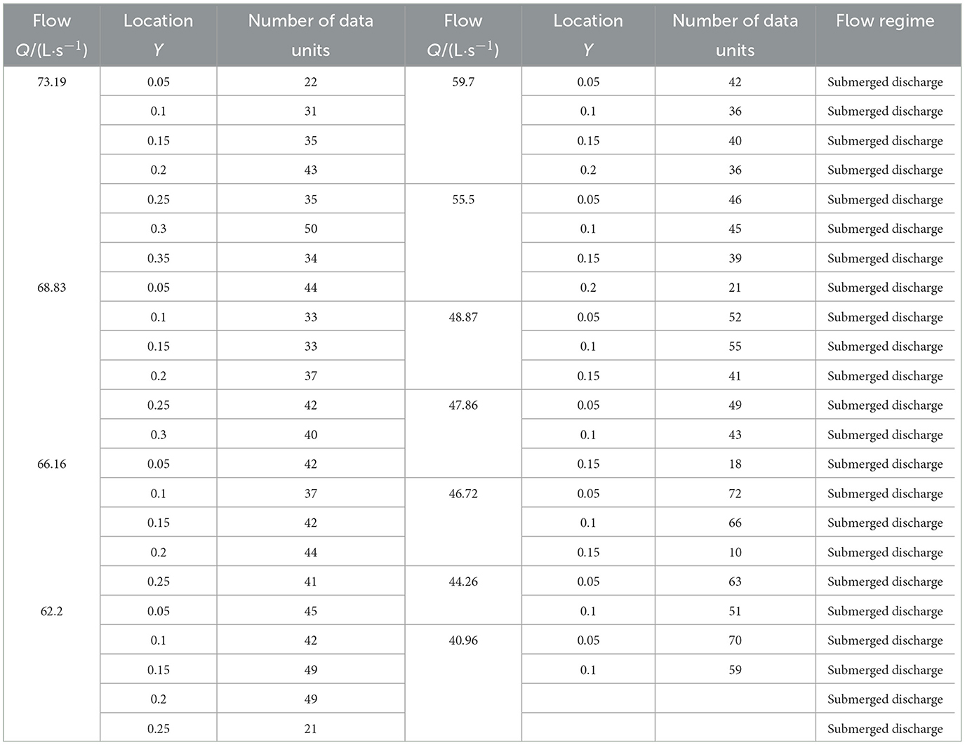
Table 1. Design experience condition table.

To verify the ultrasonic measurement of water flow velocity, five rotor current meters were evenly deployed 10 cm downstream at the same horizontal elevation as the connecting line of a pair of ultrasonic transducers. These current meters were equipped with the LGY-III multifunctional intelligent current meter developed by the Nanjing Hydraulic Research Institute. The equipment, consisting of a terminal, a main unit, and a propeller combination, was utilized to test and collect flow velocity data, with a precision of up to 0.01 cm/s.

2.2 Prediction model description

2.2.1 Ultrasonic transit time method

The principle of the transit time method in ultrasonic flowmeters (Qi et al., 2016) is that ultrasonic signals are transmitted from one transducer and are received by the other transducer after being influenced by the flow field, temperature field, and impurities in the water through multi-physical field coupling. Each transducer emits a wave signal once, and the transit time of the ultrasonic signal is used to extract flow-related information from the sound pressure (pulse) signal. The propagation times of the ultrasonic signal in the downstream and upstream directions are obtained (British Standards Institute Staff, 2017), and the fluid velocity is calculated accordingly. A schematic diagram illustrating the calculation principle of the transit time method in ultrasonic flowmeters is shown in Figure 3, and the calculation formula for the t transit time method is expressed as follows:

$\begin{array}{ll}{\widehat{V}}_i=\frac{(\frac{L}{t_1}-\frac{L}{t_2})}{2cos\theta }& (1)\end{array}$

where: ${\widehat{V}}_i$—The i-th predicted the line velocity of the water across the channel in the direction of flow, in cm·s⁻¹;

L—The path lenth(distance between transducer A and transducer B), in cm;

θ—The angle between the path and direction of flow, in °;

t₁—The transit time from transducer A to B, in μs;

t₂—The transit time from transducer B to A, in μs.

Figure 3

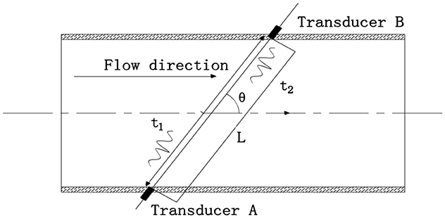
Figure 3. Schematic diagram of working and calculating principle of ultrasonic transit time method.

2.2.2 Machine learning model

2.2.2.1 Decision tree

Decision Tree (DT) regression, as a tree-structured regression model with one root node and several leaf nodes, is used to predict values. The prediction is made by recursively partitioning the input, starting from the root node to determine which leaf node the sample data should belong to. The target value of the training samples within that leaf node is then used as the predicted value. Each path from the root to a leaf node corresponds to a unique test sequence (Jung et al., 2023). In establishing the model for this experiment, the first step involves calculating the information gain index for three features (propagation time in both directions of ultrasonic transit time and speed measurement position), and ranking the feature contributions. The second step includes partitioning the dataset based on the size of the feature contributions to form sub-nodes. The third step repeats the above steps recursively for each sub-node until the stopping condition is met. The mean target value of the training samples within each sub-node, defined as ŷ_m, the calculation formula is expressed as follows:

$\begin{array}{ll}{\widehat{y}}_m=\frac{1}{N_m}{\displaystyle \sum _{i\in D_m}}{y}_i& (2)\end{array}$

Where: ŷ_m—Per leaf node target mean value;

D_m—The set of sample indices within the m-th child node;

N_m—The number of samples within the m-th child node;

y_i—Target value for the training sample associated with the i-th leaf node.

2.2.2.2 Random forest

The Random Forest model (RF), proposed by Breiman (2001) constitutes a machine learning algorithm that amalgamates the Bagging class of supervised ensemble learning algorithms with the random subspace method. It is designed to augment generalization performance through the construction of multiple decision trees and their integration. In the context of this experiment's model establishment, training data are sampled with replacement to generate several distinct datasets. Subsequently, a decision tree is constructed for each dataset, adhering to the process detailed in Section 1.2.2.1. Features are randomly selected for splitting at each leaf node's branching point, rather than considering all possible features. The final prediction value, denoted as Ŷ, is derived by averaging the predictions from each tree, the calculation formula is expressed as follows:

$\begin{array}{ll}\widehat{Y}=\frac{1}{N_{trees}}{\displaystyle \sum _{i=1}^{N_{trees}}}{f}_i(X)& (3)\end{array}$

where: Ŷ—The projected value;

N_trees—Number of trees in the model;

f_i(X)—Predicted values associated with the i-th tree.

2.2.2.3 Gradient boosting decision tree

Gradient Boosting Decision Tree (GBDT) regression is achieved by combining multiple decision trees as weak learners (Lin, 2022). The prediction error of the previous learner is calculated by the next learner, gradually reducing the model's residuals on the training data. GBDT can flexibly handle both continuous and discrete features without requiring feature transformation. During iterative computation, multiple weak learners are combined in a serial manner. For the model construction in this experiment, the first step involves the calculation of the negative gradient, which represents the residual of the current model for the previous sample. In the second step, a new weak learner is learned to fit this residual. In the third step, the learning rate is specified to control the weight of each weak learner, updating the model's predicted values. The final predictive model is the sum of the computed values of the weak learners, denoted as ŷ(x), the calculation formula is expressed as follows:

$\begin{array}{ll}\widehat{y}(x)={\displaystyle \sum _{t=1}^T}\eta h_t(x)& (4)\end{array}$

where: ŷ(x)—Accumulated value of weak learners;

η—Learning rate;

h_t(x)—Weak learners for the t-th tree.

2.2.2.4 Adaptive boosting

The Adaptive Boosting(AdaBoost) model, an ensemble learning method (Meng-ran et al., 2019), is designed to construct a strong regressor by combining multiple weak regressors to accomplish training tasks. Proposed by Yoav Freund and Robert Schapire, it is a type of Boosting algorithm. In the model establishment for this experiment, the first step involves the initialization of weight values, the training of a weak regressor, and the calculation of the error. The second step entails the readjustment of weights based on the previous calculation results, so that samples with larger errors receive more attention in the next round of training, while the weights of samples with smaller errors are reduced. The third step involves the repetition of the above process to continuously alter the weights of the samples in the learning process until the weak regressor achieves zero error. The loss function used in AdaBoost differs from that in gradient boosting tree models. The final prediction model is the cumulative value ĝ(x) calculated by the weak learners, the calculation formula is expressed as follows:

$\begin{array}{ll}\widehat{g}(x)={\displaystyle \sum _{t=1}^T}{\alpha }_t·h_t(x)& (5)\end{array}$

where: a_t—Cumulative value of the weak learner for the t-th tree;

a_t—weighted value.

2.3 Flow velocity prediction

2.3.1 The collection and pre-processing of data

The ultrasonic transit time and flow velocity data used in this experiment were stored in a MySQL database. The ultrasonic transmitter was subjected to errors due to its own track sliding and water flow during operation, necessitating the preprocessing of the raw data.

2.3.2 Outlier handling

To reduce the errors in data caused by environmental and human factors, the 3-sigma rule of normal distribution (Xiuli et al., 2023) was applied to process the propagation times of ultrasonic waves that were traveling with and against the water flow at the same location during a certain period, as shown in Figure 4. The calculation formula is expressed as follows:

$\begin{array}{ll}\mu -3\sigma <t_1,t_2<\mu +3\sigma & (6)\end{array}$

where: μ—The mean value over a certain time period;

σ—The standard deviation value over a certain time period.

Figure 4

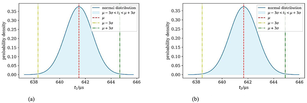
Figure 4. Sigma rule removes noisy data. (a) t₁ values are treated by the 3sigma rule. (b) t₂ values are treated by the 3 sigma rule.

2.3.3 Processing of ultrasonic transit time in the downstream and upstream flows

The ultrasonic upstream and downstream times obtained from the experiment were processed. After the outliers were filtered according to Section 1.3.2, the average propagation time in the ultrasonic upstream and downstream flow at the same location during a certain period was calculated, and the calculation formula is expressed as follows:

$\begin{array}{ll}\overline{t_s}=\frac{1}{N}{\displaystyle \sum _{i=1}^N}{t}_i& (7)\end{array}$

$\begin{array}{ll}\overline{t_n}=\frac{1}{M}{\displaystyle \sum _{i=1}^M}{t}_j& (8)\end{array}$

where: $\overline{t_s}$,$\overline{t_n}$—The average transit time of ultrasonic waves at the same position in the flow of water over a certain period of time for both downstream and upstream currents, in μs;

N,M—The amount of experimental data on the transit time of ultrasonic waves at the same position in the flow of water for both downstream and upstream currents has been collected;

t_i, t_j—The transit time of ultrasonic waves at the same location in the flow of water of the downstream and upstream currents was measured, in μs.

2.3.4 Dimensionless data processing

To eliminate the dimensional differences at measurement points affecting the model's prediction accuracy, the feature range was normalized to the [0,1] interval. In the experiment, the ultrasonic transducer and the stepper motor were fixed on a stainless steel plate for synchronous displacement. To study the flow velocity conditions at different water depths, the initial height was set when the ultrasonic transducer reached its lowest point, which was 8 cm above the channel bottom. The distance between the ultrasonic transducer and the initial position was defined as Y_i, and it was normalized with respect to the maximum displacement value Y_max, i.e. Y = Yi/Y_max. The stepper motor was controlled by a program to move 5 cm each time, and data collection began 2 min after each displacement stop, followed by another 2-min interval before the next displacement and data collection.

To effectively avoid the influence of extreme velocities in the flow field, the average value of the velocity measurements from five flow meters were taken to obtain the final research data for modeling and predicting flow velocities. After processing, 139 sets of experimental data were obtained, each set containing three independent variables (measurement position, ultrasonic transit time in both directions) and one dependent variable (flow velocity measured by the rotor flow meter). A random 70% of the samples were randomly selected with replacement from the dataset for use as the training set, while the remaining 30% of the samples were utilized as the testing set, the distribution characteristics of the data set are shown in Figure 5.

Figure 5

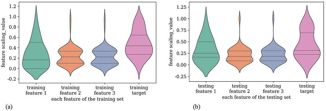
Figure 5. Distribution of feature scaling values for dataset. (a) Visualization of feature scaling values for training set. (b) Visualization of feature scaling values for testing set.

3 Results and discussion

3.1 Modeled flow velocity predictions

Based on the principle of the ultrasonic transit time method, it was determined that the location factor for ultrasonic velocity measurement could be neglected when estimating flow velocity. The flow velocity was calculated using two variables: the propagation times of ultrasound in the downstream and upstream directions. In comparison to the ultrasonic transit time method, the other four types (DT, RF, GBDT, and AdaBoost), which are categorized as machine learning models, required three variables—the propagation times of ultrasound in both downstream and upstream directions and the position of velocity measurement—to estimate the flow velocity. Consequently, this section of the discussion was bifurcated into distinct parts for transit time method predictions and machine learning model forecasts.

3.1.1 The flow velocity prediction by ultrasonic transit time method

Based on the working mechanism of the mobile ultrasonic stratified water measurement device and the principle of the ultrasonic transit time method for calculation, it can be known that after processing the transit time values of ultrasonic waves in the different directions as described in Sections 1.3.2 and 1.3.3, the predicted flow velocity values can be calculated. A linear regression was performed on these predicted values. The relative error δ [δ = |(V_measured − V_predicted )/V_measured|] between the ultrasonic transit time method predicted values and the actual measured flow velocities is shown in Figure 6a. From the figure, it can be seen that in the training set, the proportion of relative errors <5% is 31.96%, and <10% is 64.95%. In the testing set, the proportion of relative errors <5% is 28.57%, and <10% is 47.62%. The comparison between the ultrasonic transit time method predicted values and the actual measured flow velocities is shown in Figure 6b. In the figure, the x-axis represents the predicted values, which are the calculated values using the ultrasonic transit time method, and the y-axis represents the actual measured flow velocities from the flowmeter in the experiment. From the data distribution of the training and testing sets, it can be observed that the prediction effect of the ultrasonic transit time method in measuring flow velocities using the mobile ultrasonic device is not satisfactory.

Figure 6

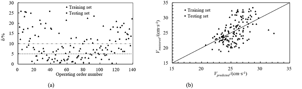
Figure 6. Prediction model of ultrasonic transit time method. (a) Absolute value of relative error. (b) Comparison of predicted and measured values.

3.1.2 Machine learning flow velocity prediction model

Based on the working mechanism of the mobile ultrasonic stratification water measurement device and the principles of machine learning, it was found that the optimal parameters for each machine learning model could be set by using the ultrasonic transit time method in both downstream and upstream flow directions and the position of velocity measurement as independent variables. These optimal parameters were determined for each model using a grid search method (Xianqing et al., 2012), machine learning model learning curves for parameters as shown in Figure 7. The optimal parameter settings for each machine learning model were presented in Table 2.

Figure 7

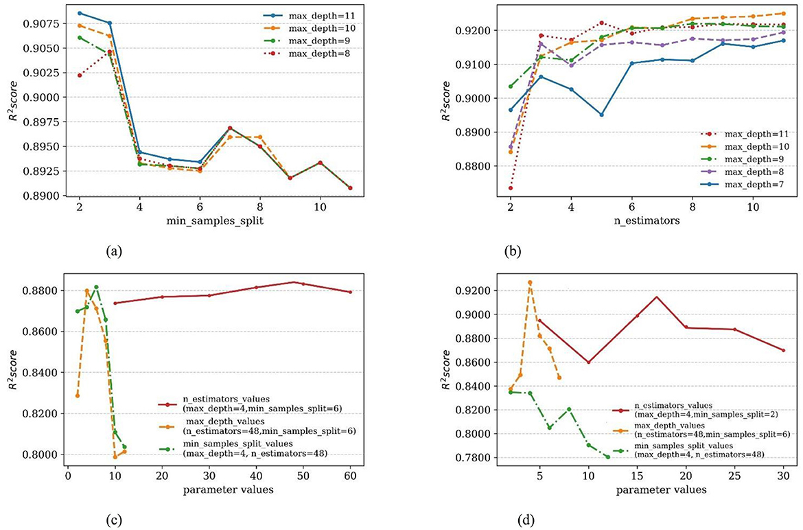
Figure 7. Machine learning model learning curves for parameters. (a) DT Learning curves for parameters. (b) AdaBoost learning curves for parameters. (c) RF learning curves for parameters. (d) GBDT learning curves for parameters.

Table 2

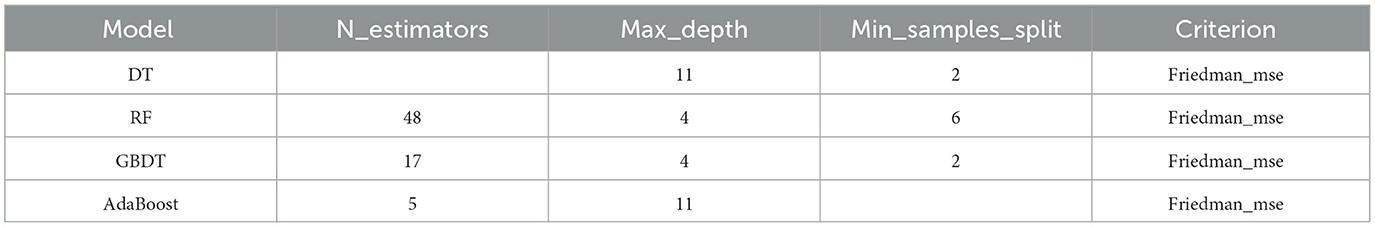
Table 2. Model grid search optimization parameters.

The same sequence dataset as the ultrasonic transit time method was utilized, and machine learning models were employed to predict the training and testing datasets. The DT, RF, GBDT, and AdaBoost prediction models calculated the relative error values. These values are depicted in Figures 8a–11a. From these figures, we can observe that, in the training set, the proportions of relative errors <5% were 100.00% for DT, 92.79% for RF, 100.00% for GBDT, and 100.00% for AdaBoost. The proportions of relative errors <10% were all 100.00% for these models. In the testing set, the proportions of relative errors <5% were 85.71%, 83.33%, 85.71%, and 85.71%, respectively, and the proportions of relative errors <10% were 95.24%, 92.86%, 95.24%, and 95.24%, respectively. The comparisons between the predicted and measured values for the DT, RF, GBDT, and AdaBoost models are shown in Figures 8b–11b. From the distribution of the training and testing datasets, it is evident that the prediction accuracy of the mobile ultrasonic device for flow velocity measurement was significantly improved compared to the ultrasonic transit time method when utilizing the DT, RF, GBDT, and AdaBoost models.

Figure 8

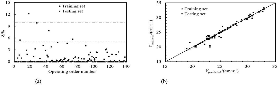
Figure 8. DT prediction model. (a) Absolute value of relative error. (b) Comparison of predicted and measured values.

Figure 9

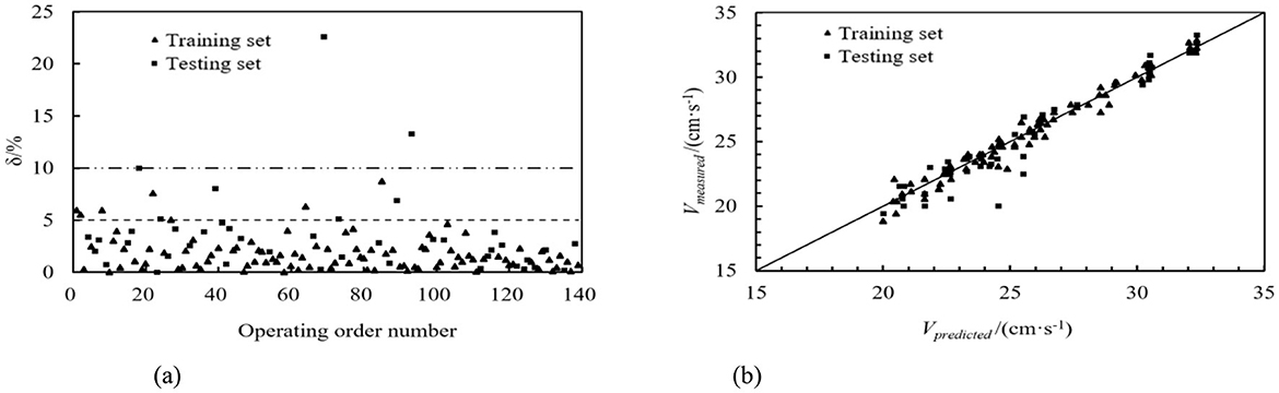
Figure 9. RF prediction model. (a) Absolute value of relative error. (b) Comparison of predicted and measured values.

Figure 10

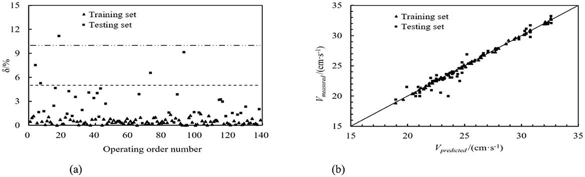
Figure 10. GBDT prediction model. (a) Absolute value of relative error. (b) Comparison of predicted and measured values.

Figure 11

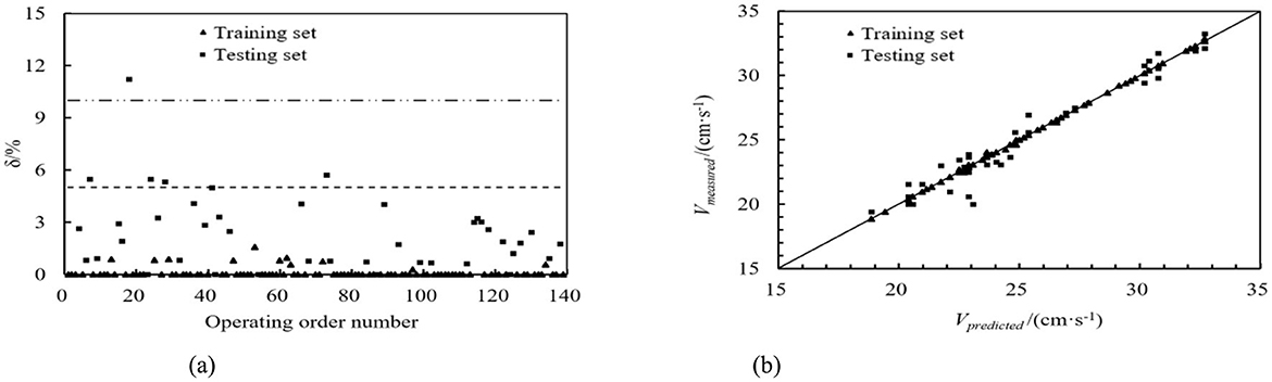
Figure 11. AdaBoost prediction model. (a) Absolute value of relative error. (b) Comparison of predicted and measured values.

3.2 Evaluation of model accuracy

Based on the calculation results presented in Section 2.1, it is found that the mobile ultrasonic transit time method for measuring flow velocity is not ideal. Consequently, this section focuses on further evaluating the machine learning models. Using the training set and testing set defined in Section 1.3.4, models are trained and tested with DT, AdaBoost, RF, and GBDT algorithms to predict flow velocity. The accuracy of the models is compared using four evaluation metrics: mean absolute error (MAE), mean squared error (MSE), root mean squared error (RMSE), and coefficient of determination (R²) (Adnan et al., 2019; Fukami et al., 2020). The best mobile ultrasonic flow velocity prediction model is determined based on these comparisons. Among these metrics, MSE, MAE, and RMSE have a range of [0, +∞], where values closer to 0 indicate better precision and fit of the model, while the R² metric has a range of [0, 1], with values approaching 1 indicating better model fit (Meng et al., 2024). The formulas for calculating each evaluation metric are expressed as shown in Equations 9–12, and the results of each metric are illustrated in Figure 12.

$\begin{array}{ll}MAE=\frac{1}{n}{\displaystyle \sum _{i=1}^n}{\displaystyle |V_i-{\widehat{V}}_i|}& (9)\end{array}$

$\begin{array}{ll}MSE=\frac{1}{n}{\displaystyle \sum _{i=1}^n}{(V_i-{\widehat{V}}_i)}^2& (10)\end{array}$

$\begin{array}{ll}RMSE=\sqrt{MSE}& (11)\end{array}$

$\begin{array}{ll}{R}^2=1-\frac{{\displaystyle {\sum }_{i=1}^n}{(V_i-{\widehat{V}}_i)}^2}{{\displaystyle {\sum }_{i=1}^n}{(V_i-\overline{V})}^2}& (12)\end{array}$

Where: V_i—The flow velocity measure value for the ith, cm·s⁻¹

n—Number of experiment groups

Figure 12

Figure 12. Model prediction evaluation parameters.

The computational results derived from Figure 12 indicated that four machine learning models were found to exhibit good predictive performance, with the R² values of the testing set decreasing in the following order: AdaBoost, DT, GBDT, and RF. The R² value of the AdaBoost model on the training set was 1.0, with an RMSE value of 0.071, an MSE value of 0.005, and an MAE value of 0.023. The R² value of the AdaBoost model on the testing set was 0.951, with an RMSE value of 0.071, an MSE value of 0.795, and an MAE value of 0.654. Compared to other machine learning models on the testing set, the AdaBoost model was found to have the highest R² value and the lowest RMSE, MSE, and MAE values, indicating the best prediction accuracy. Additionally, Taylor diagrams (Figure 13) were used to present the models as individual polar plots (Adnan et al., 2023), summarizing three key statistical indices: RMSE, standard deviation, and correlation coefficient. The model is drawn from training set and testing dataset. The Taylor diagrams of the testing set clearly shows that the correlation coefficient of AdaBoost (0.951) is higher than that of other models.

Figure 13

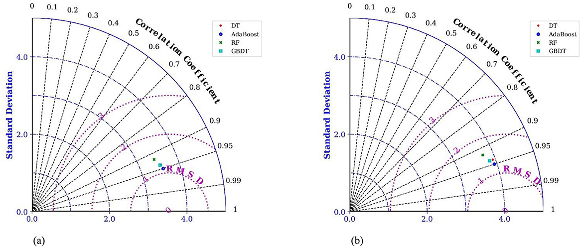
Figure 13. Taylor diagrams of the observed and predicted flow velocity by DT, AdaBoost, RF and GBDT in dataset. (a) Taylor diagram of each model in the training set. (b) Taylor diagram of each model in the testing set.

4 Discussion

This study presented a novel mobile ultrasonic stratified flow velocity measurement device, integrating machine learning algorithms to predict flow velocities in agricultural irrigation channels. The comparison of traditional ultrasonic transit time methods with machine learning-based models revealed several key findings that highlight the advantages and limitations of each approach.

4.1 Effectiveness of the mobile ultrasonic stratified flow velocity measurement device

The experimental results demonstrate that the mobile ultrasonic stratified flow velocity measurement device offers a practical and low-power solution for measuring flow velocities at multiple water depths. This device is characterized by its ability to perform velocity measurements with minimal power consumption and without introducing noise that often affects multi-channel ultrasonic flowmeters. The use of fewer ultrasonic transducers eliminates the need for complex multi-channel configurations, which are not only expensive but also prone to higher energy consumption and noise interference. Therefore, the simplicity of the device's design makes it particularly well-suited for field applications in agricultural irrigation systems, where channel sizes and flow conditions may vary.

However, the traditional ultrasonic transit time method proved to be less effective in estimating flow velocities, with notable inaccuracies in predicting water flow compared to the machine learning models. The relative error analysis showed that, while the ultrasonic transit time method predicted flow velocities with errors below 5% in only 28.57% of cases, machine learning models like AdaBoost achieved significantly better performance, with relative errors under 5% in 85.71% of cases. This suggests that the traditional ultrasonic transit time method struggles to account for the variations in flow dynamics, especially in non-ideal, variable conditions typical of agricultural channels.

4.2 Comparison of machine learning models

When comparing machine learning models (Decision Tree, Random Forest, Gradient Boosting Decision Tree, and AdaBoost), it is evident that machine learning can significantly improve the accuracy of flow velocity prediction. Specifically, AdaBoost emerged as the most effective model, outperforming other algorithms in terms of prediction accuracy and computational efficiency. The R² value for the AdaBoost model in the testing set was 0.951, which is much higher than the values obtained for the other models. Additionally, AdaBoost exhibited the lowest RMSE (0.071) and MSE (0.795), demonstrating a more robust fit and reduced prediction error compared to Decision Tree (DT), Random Forest (RF), and Gradient Boosting Decision Tree (GBDT).

The AdaBoost algorithm's superior performance can be attributed to its ability to combine weak learners to form a strong regressor, allowing it to focus more on difficult-to-predict cases by adjusting weights (Kim et al., 2008). This results in more precise predictions, even in the presence of noisy or incomplete data. Decision Trees, while effective, struggled with overfitting, which is evident from their lower performance in real-world testing scenarios.

4.3 The role of ultrasonic transit time and measurement position

The ultrasonic transit time method relied on measuring the time it takes for the ultrasonic signal to travel downstream and upstream, which is traditionally an effective way to determine flow velocity in ideal conditions (Qi et al., 2016). However, this method fails to account for the dynamic flow variations commonly found in agricultural irrigation systems, where turbulent flows and varying flow profiles can introduce significant measurement errors. Moreover, the measurement position, which varies with water depth, significantly influenced the accuracy of flow velocity predictions. This variability is more challenging to address with traditional ultrasonic methods that do not adapt to the changing environmental conditions.

By contrast, machine learning models such as AdaBoost and Random Forest incorporated additional features like measurement position and propagation times, which enabled them to capture the complexities of flow dynamics more effectively. The ability of these models to leverage multiple features allowed for more robust predictions, even when environmental factors like water turbulence or transducer misalignment introduced errors into the data.

5 Conclusion

This study focused on an experimental investigation of the velocity prediction method for mobile ultrasonic flow measurement equipment. This study comparing only with rotor flow meters, the conclusions of this research could provide a theoretical basis for water measurement applications in agricultural irrigation canals. In practical applications, the water quality in open channels was complex, and many issues remained to be studied regarding the application of measurement equipment in engineering practice. Due to limitations of time and space, the aesthetic upgrades of mobile ultrasonic measurement devices and the flow rate–area relationship will be further investigated in subsequent studies. The key findings are summarized as follows:

(1) The experiment results show that the traditional ultrasonic transit time method was not effective in calculating water flow velocity with mobile ultrasonic transducers. The proportion of predicted flow velocities with a relative error <5% in the test dataset was 28.57%, which did not meet the relevant hydraulic standards.

(2) By using the positions of the ultrasonic transducer measurements and the transit times of ultrasound in both downstream and upstream directions as independent variables, further research was carried out using machine learning models such as DT, RF, GBDT, and AdaBoost. After grid search optimization of the model parameters, these four models were utilized to predict the flow velocity. The machine learning models were found to perform better than the traditional ultrasonic transit time method. Among the four machine learning models, the proportions of predicted flow velocities with a relative error <5% from highest to lowest were: AdaBoost (85.71%), DT (85.71%), GBDT (85.71%), and RF (83.33%).

(3) For the AdaBoost model, the R² value for the training set was reported as 1.0, RMSE was 0.071, MSE was 0.005, and MAE was 0.023; in the testing set, the AdaBoost model had the highest R² value at 0.951 compared to other machine learning models, and the smallest values for the other three evaluation metrics: RMSE was 0.071, MSE was 0.795, and MAE was 0.654. It was evident that the AdaBoost model had higher prediction accuracy and a better fit compared to other machine learning models, making it more suitable for mobile ultrasonic flow measurement equipment.

The study also presents several limitations that require further attention in future research. First, the performance of the device was only validated using the rotor flow meter, and the experimental conditions were somewhat limited, focusing on a specific range of flow velocities and flow conditions. Therefore, future studies should expand the experimental scope to include a wider range of flow velocities, water qualities, and environmental conditions to assess the broader applicability of the model. In terms of algorithms, while AdaBoost showed excellent performance, other advanced machine learning algorithms, such as deep learning models and support vector machines, may offer further improvements in prediction accuracy. Future work should consider a comprehensive comparison of various machine learning algorithms and optimize the current models to improve the overall performance of the device.

In conclusion, while the mobile ultrasonic stratified flow velocity measurement device demonstrated clear advantages in terms of accuracy and low power consumption, challenges remain in real-world applications, particularly in dealing with fluctuating water quality and dynamic flow conditions. Future research will focus on optimizing measurement algorithms, enhancing device performance, and exploring broader applications in agricultural irrigation.

Data availability statement

The datasets presented in this article are not readily available because the data that support the findings of this study are available on request from the corresponding author, Chunliang Cui, upon reasonable request. Requests to access the datasets should be directed to eGpza3lwc3lAMTYzLmNvbQ==.

Author contributions

SP: Funding acquisition, Methodology, Writing – original draft, Writing – review & editing. HL: Methodology, Software, Visualization, Writing – review & editing. YB: Investigation, Visualization, Writing – review & editing. ZC: Data curation, Validation, Writing – review & editing. JY: Data curation, Investigation, Software, Writing – review & editing. CC: Conceptualization, Project administration, Resources, Software, Supervision, Writing – review & editing.

Funding

The author(s) declare that financial support was received for the research and/or publication of this article. This work was supported by the Natural Science Foundation Project of Xinjiang Uygur Autonomous Region (2024D01A99), the National Natural Science Foundation of China (72304245), the Major Science and Technology Project of the Xinjiang Uygur Autonomous Region (2022A02003-5), the Special Program for Hydraulic Science and Technology of Xinjiang Uygur Autonomous Region (XSKJ-2023-25), the Key Talent Training Project “Three Rural Areas” in Xinjiang (2022SNGGGCC008), the “Light of West China” Program of the Chinese Academy of Sciences (Rc924003), and Public Welfare Research Institutes of Xinjiang Uygur Autonomous Region (KY2024082).

Conflict of interest

The authors declare that the research was conducted in the absence of any commercial or financial relationships that could be construed as a potential conflict of interest.

Generative AI statement

The author(s) declare that no Generative AI was used in the creation of this manuscript.

Publisher's note

All claims expressed in this article are solely those of the authors and do not necessarily represent those of their affiliated organizations, or those of the publisher, the editors and the reviewers. Any product that may be evaluated in this article, or claim that may be made by its manufacturer, is not guaranteed or endorsed by the publisher.

References

Adnan, R. M., Liang, Z., Trajkovic, S., Zounemat-Kermani, M., Li, B., and Kisi, O. (2019). Daily streamflow prediction using optimally pruned extreme learning machine. J. Hydrol. 577, 1–11. doi: 10.1016/j.jhydrol.2019.123981

Crossref Full Text | Google Scholar

Adnan, R. M., Mirboluki, A., Mehraein, M., Malik, M., Heddam, S., and Kisi, O. (2023). Improved prediction of monthly streamflow in a mountainous region by Metaheuristic-Enhanced deep learning and machine learning models using hydroclimatic data. Theoret. Appl. Climatol. 155, 205–228. doi: 10.1007/s00704-023-04624-9

Crossref Full Text | Google Scholar

Adnan, R. M., Mostafa, R. R., Wang, M., et al. (2025). Improved random vector functional link network with an enhanced remora optimization algorithm for predicting monthly streamflow. J. Hydrol. 650, 1–24. doi: 10.1016/j.jhydrol.2024.132496

Crossref Full Text | Google Scholar

Afaridegan, E., and Amanian, N. (2025). Enhanced prediction of energy dissipation rate in hydrofoil-crested stepped spillways using novel advanced hybrid machine learning models. Results Eng. 25, 1–23. doi: 10.1016/j.rineng.2025.103985

Crossref Full Text | Google Scholar

Bahrami, S., Alamdari, S., Farajmashaei, M., Behbahani, M., Jamshidi, S., and Bahrami, B. (2024). Application of artificial neural network to multiphase flow metering: a review. Flow Measurem. Instrument. 97, 1–25. doi: 10.1016/j.flowmeasinst.2024.102601

Crossref Full Text | Google Scholar

Breiman, L. (2001). Random forests. Mach. Learn. 45, 5–32. doi: 10.1023/A:1010933404324

Crossref Full Text | Google Scholar

British Standards Institute Staff (2017). Hydrometry-Measurement of Discharge by the Ultrasonic Transit Time (Time of Flight) Method:ISO 6416-2017. London: British Standards Institution (BSI).

Google Scholar

Chapa, J. O., and Rao, R. (2001). Algorithms for designing wavelets to match a specified signal. Trans. Signal Proc. 48, 3395–3406. doi: 10.1109/78.887001

Crossref Full Text | Google Scholar

Chen, J., Zhang, K., Wang, L., and Yang, M. (2020). Design of a high precision ultrasonic gas flowmeter. Sensors 20, 1–15. doi: 10.3390/s20174804

PubMed Abstract | Crossref Full Text | Google Scholar

Fukami, K., Fukagata, K., and Taira, K. J. T. (2020). Assessment of supervised machine learning methods for fluid flows. Theoret. Comput. Fluid Dynam. 34, 497–519. doi: 10.1007/s00162-020-00518-y

Crossref Full Text | Google Scholar

Guolong, Z., Junxi, J., Qiangxue, W., and Shaoqing, N. (2022). Development of all-plastic short tube ultrasonic water meter with adjustable core tube Angle. J. Irrigat. Drain. 41, 51–56. doi: 10.13522/j.cnki.ggps.2022046

Crossref Full Text | Google Scholar

Huang, S. Y., Guo, Y. Q., Zang, X. L., and Xu, Z. (2024). Design of ultrasonic guided wave pipeline non-destructive testing system based on adaptive wavelet threshold denoising. Electronics 13, 1–19. doi: 10.3390/electronics13132536

Crossref Full Text | Google Scholar

Iooss, B., Lhuillier, C., and Jeanneau, H. (2002). Numerical simulation of transit-time ultrasonic flowmeters: uncertainties due to flow profile and fluid turbulence. Ultrasonics 40, 1009–1015. doi: 10.1016/S0041-624X(02)00387-6

PubMed Abstract | Crossref Full Text | Google Scholar

Jackson, G. A., Gibson, J. R., and Holmes, R. A. (1989). three-path ultrasonic flowmeter for small-diameter pipelines. J. Phys. E Sci. Instrum. 22, 645–650. doi: 10.1088/0022-3735/22/8/022

Crossref Full Text | Google Scholar

Jianfei, G., Yuyu, C., and Ya, G. (2023). Research on ultrasonic process fusing tomography for numerical and laboratory imaging in liquid-background two-phase flow. Appl. Acoust. 205, 1–25. doi: 10.1016/j.apacoust.2023.109278

Crossref Full Text | Google Scholar

Jie, S., Jing, Y., Shujie, D., Shaboo, L., and Jianjun, H. (2024). Hyperspectral image classification based on multi-attention mechanism and compiled graph neural network. Trans. Chin. Soc. Agricult. Machine. 55, 183–192+212.

Google Scholar

Jung, W. S., Jo, B. G., and Kim, Y. D. A. (2023). Study on the occurrence characteristics of harmful blue-green algae in stagnant rivers using machine learning. Applied Sci. 13, 2076–3417. doi: 10.3390/app13063699

Crossref Full Text | Google Scholar

Kim, J. H., Kwon, B. G., Kim, J. Y., and Kang, D. J. (2008). “Method to improve the performance of the adaboost algorithmby combining weak classifiers,” in International Workshop on Content-Based Multimedia Indexing, 357–364. doi: 10.1109/CBMI.2008.4564969

Crossref Full Text | Google Scholar

Lee, J., Kim, M., and Park, H. (2021). Single-layer wire-mesh sensor to simultaneously measure the size and rise velocity of micro-to-millimeter sized bubbles in a gas-liquid two-phase flow. Int. J. Multiphase Flow 139, 1–26. doi: 10.1016/j.ijmultiphaseflow.2021.103620

Crossref Full Text | Google Scholar

Lin, L. (2022). Disease Prediction Analysis Based on Optimal Random Forest Mixture Model. Zhengzhou: North China University of Water Resources and Electric Power.

PubMed Abstract | Google Scholar

Ling, C. (2007). Application and development of new flow measuring Instrument. Transdu. Microsyst. 6, 8–11.

Google Scholar

Ling, L., and Fusheng, G. (2005). Numerical Calculation Method. New York, NY: Science Press.

Google Scholar

Longhui, Q. (2016). Intelligent Algorithm for Multi-Channel Ultrasonic Flow Calculation and Flow Field Profile Recognition. Hangzhou: Zhejiang University.

Google Scholar

Luntta, E., and Halttunen, J. (1999). Neural network approach to ultrasonic flow measurements. Flow Measurem. Instrument. 10, 35–43. doi: 10.1016/S0955-5986(98)00035-1

Crossref Full Text | Google Scholar

Meng, L., Yan, Y., Jing, H., Baloch, M. Y. J., Du, S., and Du, S. (2024). Large-scale groundwater pollution risk assessment research based on artificial intelligence technology: a case study of Shenyang City in Northeast China. Ecol. Indic. 169, 1–17. doi: 10.1016/j.ecolind.2024.112915

Crossref Full Text | Google Scholar

Meng-ran, Z., Da-tong, L., Feng, H., Wen-hao, L., Ya, W., and Song, Z. (2019). Research of AdaBoost algorithm in fluorescence spectrum identification of mine water inrush source. Spectrosc. Spectral Analy. 39, 485–490. doi: 10.3964/j.issn.1000-0593(2019)02-0485-06

Crossref Full Text | Google Scholar

Pannell, C. N., Evans, W. A. B., and Jackson, D. A. A. (1990). new integration technique for flowmeters with chordal paths. Flow Measurem. Instrument. 1, 216–224. doi: 10.1016/0955-5986(90)90016-Z

Crossref Full Text | Google Scholar

Pereira, T. S. R., de Carvalho, T. P., Mendes, T. A., and Formiga, K. T. (2022). Evaluation of water level in flowing channels using ultrasonic sensors. Sustainability 14, 1–15. doi: 10.3390/su14095512

Crossref Full Text | Google Scholar

Qi, L., Yongxing, W., Jie, L., and Huayi, C. (2016). Acoustic field analysis and research of ultrasonic wind measurement system based on time-lag method. J. Marine Technol. 35, 68–73. doi: 10.3969/j.issn.1003-2029.2016.01.011

Crossref Full Text | Google Scholar

Rongxiang, H., Yadong, Z., and Shizong, Z. (2018). Research on measurement method of water metering facilities in irrigation district. J. Irrigat. Drain. 37, 13–15. doi: 10.13522/j.cnki.ggps.2017.0638

Crossref Full Text | Google Scholar

Sun, T., and Zhao, K. (2012). A review of domestic and international research on the efficiency evaluation of agricultural irrigation water use. J. Water-saving Irrig. 2012, 67–71.

Google Scholar

Sun, Y., Zhang, T., and Zheng, D. (2018). New analysis scheme of flow-acoustic coupling for gas ultrasonic flowmeter with vortex near the transducer. Sensors 18, 1–22. doi: 10.3390/s18041151

PubMed Abstract | Crossref Full Text | Google Scholar

Tongfu, L., Zhaomin, K., and Xiunan, F. (2013). Numerical Calculation Method. Beijing: Tsinghua University Press.

Google Scholar

Voser, A. (1999). Analyse und Fehleroptimierung der mehrpfadigen akustischen Durchflussmessung in Wasserkraftanlagen. Zurich: ETH Zurich

Google Scholar

Wang, M., Liu, J., Bai, Y., et al. (2023). Flow rate measurement of gas-liquid annular flow through a combined multimodal ultrasonic and differential pressure sensor. Energy 288, 1–17. doi: 10.1016/j.energy.2023.129852

Crossref Full Text | Google Scholar

Xianqing, L., Hongwei, H., Yujun, X., Jishun, L., and Mingde, D. (2012). Grid search algorithm for sphericity error. Trans. Chin. Soc. Agricult. Machine. 43, 222–225. doi: 10.6041/j.issn.1000-1298.2012.05.038

Crossref Full Text | Google Scholar

Xiaoyu, T., Hongjian, Z, Xiang, X., and Hongliang, Z. (2017). Model simulation and experimental study on effect of acoustic plane installation angle on measurement of multi-channel ultrasonic gas flowmeter. J. Central South Univers. 48, 1923–1929. doi: 10.11817/j.issn.1672-7207.2017.07.032

PubMed Abstract | Crossref Full Text | Google Scholar

Xiuli, Z., Na, Q., Dawei, W., and Jinyou, Q. (2023). Prediction of effect of mechanical compaction on soybean yield based on Machine learning. Trans. Chin. Soc. Agricult. Machine. 54, 139–147. doi: 10.13427/j.cnki.njyi.20240018.017

Crossref Full Text | Google Scholar

Xucun, W., Rong, W., and Jiadong, M. (2023). Application of ultrasonic flowmeter in Yanghuang Channel. J. Irrigat. Drain. 42, 90–97. doi: 10.13522/j.cnki.ggps.2022465

Crossref Full Text | Google Scholar

Yuezhong, L. (2010). Research on Key Technologies of Multi-Channel Ultrasonic Gas Flow Measurement. Wuhan: Huazhong University of Science and Technology.

Google Scholar

Zhang, H., Guo, C., and Lin, J. (2019). Effects of velocity profiles on measuring accuracy of transit-time ultrasonic flowmeter. Appl. Sci. 9, 1–11. doi: 10.3390/app9081648

Crossref Full Text | Google Scholar

Zhao, H., Peng, L., Takahashi, T., and Hayashi, T. (2014). Support vector regression-based data integration method for multipath ultrasonic flowmeter. Trans. Instrument. Measurem. 63, 2717–2725. doi: 10.1109/TIM.2014.2326276

Crossref Full Text | Google Scholar

Zhen, W., Haibo, Z., Tao, M., Dupont, P., Roussette, O., Fammery, S., et al. (2013). Experimental study on measurement performance of dual channel ultrasonic flowmeter under choke condition. Indust. Metrol. 23, 33–36. doi: 10.13228/j.boyuan.issn1002-1183.2013.04.016

Crossref Full Text | Google Scholar

Zheng, D., Zhao, D., and Mei, J. (2015). Improved numerical integration method for flowrate of ultrasonic flowmeter based on Gauss quadrature for non-ideal flow fields. Flow Measurem. Instrument. 2015, 28–35. doi: 10.1016/j.flowmeasinst.2014.10.005

Crossref Full Text | Google Scholar