A hybrid statistical-dynamical forecast of seasonal streamflow for a catchment in the Upper Columbia River basin in Canada

We explore a hybrid statistical-dynamical approach as a methodology for potentially improving total seasonal streamflow volume forecasts at a key lake reservoir in the Upper Columbia River basin, a region vital for hydroelectric power generation in British Columbia. Seasonal streamflow forecasts in this basin at early or mid-winter initialization times often exhibit limited skill due to the lack of snowpack information in the initial conditions. Our method integrates temperature and precipitation data from the ECMWF seasonal forecasts (SEAS5) with a Long Short-Term Memory (LSTM) neural network. To our knowledge, this is the first time an LSTM has been used specifically for predicting total seasonal streamflow volume in this basin. When forced with reanalysis data (ERA5), the LSTM model performs substantially better at predicting total seasonal streamflow when trained and applied at a monthly timescale, as compared to the more typical daily timescale used in previous streamflow LSTM applications. In the case study region, when forecasts are initialized on 1 January, only three months of meteorological forecast skill are needed to achieve strong predictive skill of total seasonal streamflow (R² > 0.7), attributed to accurate representation of snowpack build up in the winter months. The hybrid forecast, with the LSTM forced by SEAS5 data, tends to underestimate seasonal volumes in most years, primarily due to biases in the SEAS5 input data. While bias correction of the inputs improves model performance, no skill beyond that of a forecast with average meteorological conditions as input is achieved. The effectiveness of the hybrid approach is constrained by the accuracy of seasonal meteorological forcings, although the methodology shows potential for improved predictions of seasonal streamflow volumes if seasonal meteorological forecasts can be improved.

1 Introduction

On seasonal timescales, forecasting of streamflow is important for planning and water management, particularly in the hydroelectricity sector, where decisions can have great economic and environmental impacts. The Columbia River in British Columbia (BC) generates about a quarter of the province's electricity through hydroelectricity dams in its basin, and also flows in the United States. The first dam along the river, Mica, regulates streamflow into stations downstream, thus forecasting of streamflow entering the Kinbasket Lake Reservoir that feeds into the Mica dam is essential for electricity production in BC. In this work, we develop a novel streamflow forecast method to predict seasonal total streamflow at Mica.

The Columbia River originates in the Rocky Mountains, and the Kinbasket Lake Reservoir and Mica dam are within this mountainous area. For forecasting streamflow in mountainous catchments such as this, studies have highlighted the importance of winter snowpack for spring streamflow levels (Arnal et al., 2018) and glacier melt for summer streamflow levels (Jost et al., 2012). In the Columbia River basin, previous research investigating seasonal forecasting has studied the effects of modes of interannual climate variability (e.g. El Niño Southern Oscillation, ENSO, or the Pacific Decadal Oscillation, PDO) on snowpack (Hsieh and Tang, 2001) and streamflow (Gobena et al., 2013; Hamlet and Lettenmaier, 1999) or combined information about the state of these modes with existing forecast systems (Hamlet et al., 2002). Many studies focus on stations in the portions of the Columbia River basin in southern BC and the United States, tens of kilometers downstream of Mica and not within the Rocky Mountains (e.g. Hamlet and Lettenmaier, 1999; Hsieh et al., 2003).

Most current operational streamflow forecasts, including those at Mica, use dynamical and/or statistical models of the weather, hydrological system, or both (Wood et al., 2019). Dynamical models (also called numerical models) use equations to represent physical processes describing the evolution of a system (weather or hydrological conditions), numerically modeling these processes, and their impacts, over time (Slater et al., 2023). Dynamical weather models aim to predict the evolution of the atmosphere, and sometimes ocean and land surface as well. Dynamical hydrological models typically consist of a land surface hydrological model initialized with observed current conditions and forced by weather data. These weather data can be output from numerical models (Yuan et al., 2015; NOAA, 2016) or historical weather data (Day, 1985; van Dijk et al., 2013). Although dynamical models are representative of physical processes, limitations in their predictive skill remain (Arnal et al., 2018), including representations of atmospheric teleconnections, i.e. the remote impacts of localized changes (Schepen et al., 2016; Strazzo et al., 2019), and parameterization of sub-grid scale processes. Dynamical models often require large amounts of computational resources for running and calibration (Slater et al., 2023; Arheimer et al., 2020). Dynamical forecasts are especially popular for streamflow prediction in snowmelt-dominated mountainous catchments (Araya et al., 2023), as they can incorporate initial hydrological conditions, such as snowpack, that can strongly influence the spring and summer streamflow response. However, the reliance on initial conditions means that it can be difficult for these dynamical models to forecast streamflow from early-winter initialization times when there is little snowpack present (Araya et al., 2023).

In contrast to the dynamical, process-based models described above, statistical, data-driven models require no prior knowledge of the relevant physics—they utilize large amounts of data to find connections between variables. This flexibility can be especially useful when relationships between variables are not entirely understood; however, it can result in challenges when attempting to predict physically plausible extremes not previously observed in the training datasets (Slater et al., 2023; Frame et al., 2022). For applications in modeling streamflow, deep learning-based models have been shown to outperform dynamical models in numerous basins and flow regimes (Kratzert et al., 2019; Lees et al., 2021). In particular, Long Short-Term Memory (LSTM) neural networks have been proven a useful modeling tool for streamflow in different regions, including in the United States (Kratzert et al., 2018, 2019), Europe (Lees et al., 2021), and western Canada (Anderson and Radić, 2022). Applications of LSTM models for forecasting streamflow into the future (beyond one day lead forecasts) typically fall under the category of hybrid forecasting, as they utilize dynamical forecasts of meteorological conditions as well.

Hybrid forecasting, where dynamical and statistical models are combined, is becoming popular to increase predictive skill of hydrological variables. Hybrid forecasts take advantage of the computational power of data-driven methods while retaining the sources of predictability in dynamical methods. Slater et al. (2023) provide a comprehensive review of hybrid forecasting in hydrology, highlighting the current advantages and limitations. Hybrid statistical-dynamical forecasts combine dynamical forecasts of meteorological conditions with data-driven hydrological forecasting methods (Slater et al., 2023). Hybrid forecasts with LSTMs have generally performed well when compared to benchmark dynamical hydrological models, for example by Hunt et al. (2022) in the western United States with five days lead time, and by Hauswirth et al. (2023) in the Netherlands with several months lead time. These studies, however, do not test hybrid forecasts for predicting seasonal total streamflow, a variable that is useful for hydroelectric operations.

In this study, we apply the hybrid statistical-dynamical method with an LSTM to forecast streamflow on seasonal timescales at the Kinbasket Lake Reservoir and Mica dam (referred to as “Mica catchment” from now on), and test its ability to simulate seasonal total January to September streamflow volume (“seasonal volume”) at nine months lead time, i.e. initialized 1 January. We hypothesize that a hybrid statistical-dynamical forecast may have predictive skill at this initialization time by combining the long-term memory retention of the LSTM with meteorological forecasts. There are few studies that address hybrid forecasting with seasonal lead times, and to our knowledge, this is the first study to investigate seasonal volume forecasting using a hybrid LSTM model in this basin.

The paper is structured in the following way: in Section 2, we describe the study region, datasets used, the LSTM architecture and hybrid forecast design; Section 3 presents the results of the LSTM model and the hybrid forecasts; discussion of the results is presented in Section 4; and in Section 5, we present a summary and conclusions.

2 Data and methods

2.1 Study region

The Mica catchment, located in the Rocky Mountains, is snowmelt-dominated and thus its annual streamflow has a very strong seasonal cycle, with little streamflow in the winter months and very high streamflow in late spring to summer due to snowmelt. There is also some glacier contribution that maintains high streamflow levels into the late summer (Jost et al., 2012). Figure 1 presents the annual streamflow at Mica station averaged over 1982–2017 (Figure 1a), the annual temperatures and precipitation in the Mica catchment averaged over 1981–2017 (Figures 1b, c), as well as the location of the basin (Figure 1d).

Figure 1

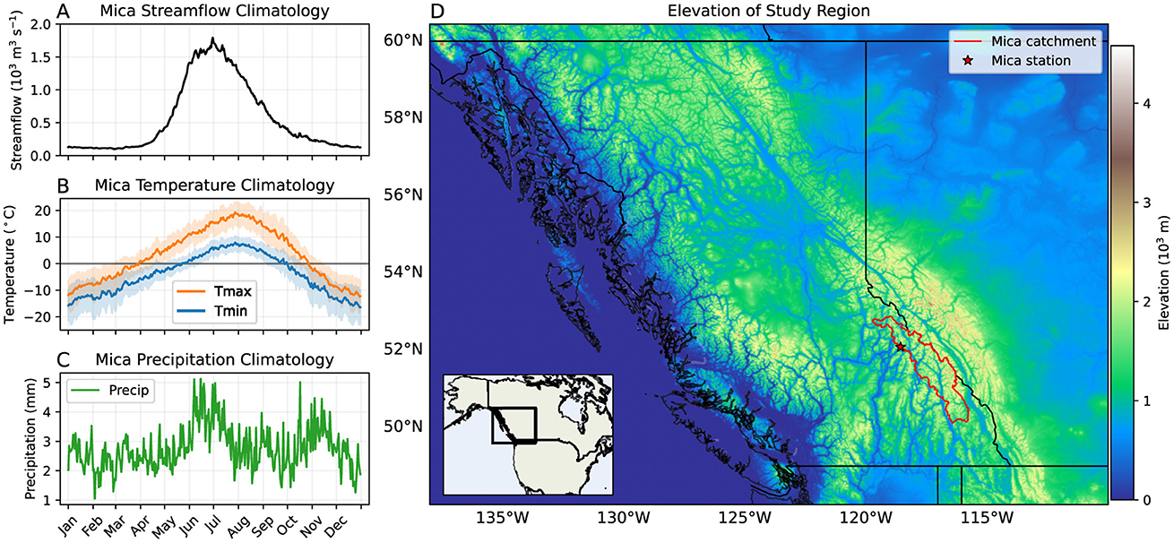
Figure 1. The Mica catchment. (A) The annual modified streamflow measured at Mica station (Dakhlalla et al., 2020), averaged over 1982–2017. (B) The annual daily minimum temperature (Tmin) and maximum temperature (Tmax) from ERA5 (Hersbach et al., 2020), averaged over 1981–2017 and the Mica catchment area. (C) The annual daily precipitation (Precip) from ERA5 (Hersbach et al., 2020), averaged over 1981–2017 and the Mica catchment area. (D) Elevation of the study region from the NOAA ETOPO Global Relief Model (NOAA, 2022). The Mica catchment area is outlined in red, the Mica station location is indicated by a red star. The provincial borders of British Columbia and Alberta are shown in black. The inset shows the study region in the context of North America.

2.2 Streamflow data

We use daily inflow from 1982–2017 at Mica station (118.57°W, 52.08°N) from the Bonneville Power Administration 2020 Level Modified Streamflow dataset (Dakhlalla et al., 2020). In this dataset, the raw observed flow values have been modified to account for current irrigation depletions and river regulations, and therefore the modified values represent streamflow that would have been observed in the past with irrigation and regulations of 2018 (Dakhlalla et al., 2020). This enables these past values to be used to predict the future in which there are regulations like those of 2018. Streamflow observations at Mica were provided to the Bonneville Power Administration by the project owner (BC Hydro), and missing data were estimated using linear regression from nearby stations (Dakhlalla et al., 2020). Irrigation depletions were calculated by Washington State University, with demand calculated through a crop water demand model (Hills et al., 2020), although this was small for the upper Columbia River area, including the Mica catchment, due to little agriculture. Daily inflow values are provided in cubic feet per second, and we convert to cubic meters per second. We convert daily streamflow to monthly streamflow volume by multiplying by the number of seconds in a day (864,400 s) and summing all days in each month.

2.3 Meteorological data

Following Anderson and Radić (2022), who used LSTM models to simulate daily streamflow across western Canada, we assume that temperature and precipitation are sufficient inputs to the LSTM model. For the dynamical forecast part of our hybrid model, we use SEAS5 seasonal hindcasts from ECMWF (Johnson et al., 2019), from 1981 to 2017. SEAS5 is the fifth generation of ECMWF's seasonal forecasting system. The hindcasts (also known as re-forecasts) are initialized every month in 1981–2017 with 25 ensemble members using the same SEAS5 forecasting system as their real-time forecasts, providing hindcasts (the forecast that would have been made at that time, if the forecast model had existed) of meteorological variables that can be compared to historical observations (Johnson et al., 2019). We download minimum temperature (Tmin), maximum temperature (Tmax), and accumulated precipitation (Precip) as monthly values at 1° × 1° spatial resolution. Grid cells within the Mica catchment area (11 grid cells) are averaged together to create one value for each time and each variable. Grid cells are not weighted based on the fraction of area contained within the basin; although we acknowledge this could introduce bias, we expect this bias to be low due to our analysis of different resolutions of data. We select hindcasts initialized 1 January, and download data for January through to June, i.e. with lead times of 1–6 months (with 6 months lead time the maximum available for this hindcast dataset).

The LSTM model is trained on ERA5 reanalysis data (Hersbach et al., 2020). We download hourly surface temperature at 2 m height (“2m temperature”) and precipitation, available at 0.25° horizontal resolution, for the period 1981–2017. The data are aggregated to daily Tmin, Tmax, and Precip. In addition, we calculate monthly mean Tmin and Tmax by taking the mean of daily Tmin and Tmax over all days in each month, and monthly accumulated Precip by summing the precipitation in all days of each month. We choose to use mean daily Tmin and Tmax over each month rather than the minimum and maximum of daily temperature values in each month to represent average temperature in the catchment for each month. The ERA5 data are regridded to the 1° × 1° spatial resolution of the SEAS5 hindcasts using Climate Data Operators (Schulzweida, 2023). Tmin and Tmax are regridded bilinearly and conservative mapping is used for Precip. Similarly to SEAS5, the grid cells within the Mica catchment (11 grid cells) are averaged together to produce one value for each day/month and each variable.

2.4 Long Short-Term Memory (LSTM) neural network

Here we briefly describe the LSTM model architecture (additional details can be found in Kratzert et al. (2018)), followed by the model set-up, training and evaluation. In general, neural network models aim to approximate functions that connect input data (e.g. meteorological data), represented by input neurons, to output or target data (e.g. streamflow data), represented by output neurons, through a series of hidden layers, each containing hidden neurons. The training of these models, i.e. the tuning of model parameters in the functions interconnecting each layer, aims to minimize the distance between model output and observed target data. The LSTM network is a type of recurrent neural network (RNN), where information between input and output layers flows in both directions through cycles and loops so that the model can learn long-term dependencies in sequential data. This is done through a second cell state that stores memory of the network, in addition to the internal hidden state in a typical RNN. The input x is a vector of the last n consecutive timesteps of meteorological forcings, x = [x₁, ..., x_n], where each x_i is itself a vector of length equal to the number of forcings (three in this study: Tmin, Tmax, Precip). For each time step t (1 ≤ t ≤ n), a series of gates update both the cell and internal states, controlling the information flow. These include the forget gate, potential cell update, input gate, and output gate. The cell state (“long-term memory”) is updated from the results of the forget gate, potential update vector, input gate, and cell state of the previous time step, while the hidden state (“short-term memory”) is updated from the cell state and the results of the output gate. Finally, the output from the final hidden state at the last time step is passed through a dense layer, where it is linearly transformed into a value of normalized streamflow (output data).

Following Anderson and Radić (2022), the model is designed to include one LSTM layer followed by one dense layer, with hidden and cell state vector lengths of 80 units, a mean squared error loss function, Adam optimization (Kingma and Ba, 2017), a learning rate of 10⁻⁴, and batch size of 64. The coding was done in Python (Van Rossum and Drake, 2009) using the Keras (Chollet, 2015) and TensorFlow (Abadi et al., 2015) libraries. The impact of the addition of a second LSTM layer into the model was also investigated (see Section 3.1 for further discussion), although further modifications to LSTM model architecture are outside the scope of this work.

Initially the model was set to predict daily streamflow using daily input data from the previous n (365) days, to predict streamflow at the day n+1. However, as we are interested in seasonal streamflow and not daily variations, we also design an LSTM model that is forced with monthly input data, using n previous months, to predict the monthly streamflow volume at the month n+1. For the monthly LSTM model, we also explore the sensitivity of the modeled streamflow to the choice of n, i.e. n = 12, 24, and 36 months. Thus, our daily LSTM model has input size of 365 × 3 neurons, and our monthly model has input size of n×3, where n = 12, 24, or 36. The training, validation, and testing data are normalized (subtracted mean and divided by standard deviation) relative to the selected training data, for each variable separately.

For each model (daily and monthly), we train five different ensemble members, each initialized with different random weights, but trained, validated, and tested on the same data. We calculate the ensemble average and standard deviation of the outputs across these five ensemble members. To maximize the available testing data within our relatively short data availability period, we use a leave-1-year-out testing method. Each year in the input data, from 1982 to 2017, is taken in turn as the test year, with training and validation years chosen randomly from the remaining years (28 for training and 7 for validation). This method ensures the largest possible number of years to evaluate the ability of this LSTM to predict seasonal volumes, as we have 36 different test years.

The predicted total volume from the beginning of January to the end of the water year at the end of September (“seasonal volume”) is calculated from the denormalized LSTM model outputs for each test year. For the daily LSTM model, this is calculated by summing daily streamflow values (in m³) over all days from 1 January to 30 September. For the monthly LSTM model, this is calculated by summing all predicted monthly volumes (in m³) from January to September. These predicted seasonal volumes are then compared to observed seasonal volumes.

To evaluate the sensitivity of results to the random selection of training and validation years in each model, model training and testing is repeated five times. In each case, testing is performed on the same test years (1982–2017), but the random training and validation years chosen from the remaining years may differ in selection and order.

Both the daily and monthly LSTM models were trained and tested using ERA5 data. Once the monthly LSTM model was trained, it was also driven by the dynamical seasonal meteorological forecast data. Given the known biases between the seasonal forecast and ERA5 (see Section 3.3), we also tested the model using bias-corrected seasonal forecasts. Two commonly used bias correction methods were selected for this purpose (von Storch and Zwiers, 1999): a linear mean shift of the SEAS5 hindcasts to align with the mean of ERA5 and a quantile–quantile bias correction to map the cumulative distribution function of the SEAS5 hindcasts onto that of ERA5 (White and Toumi, 2013). For the linear shift bias correction, the SEAS5 hindcast temperature or precipitation for each month was adjusted linearly to match the corresponding mean of ERA5. In the quantile–quantile bias correction, for each month and each variable, the SEAS5 hindcasts and ERA5 reanalysis data from 1981 to 2017 were ranked. The SEAS5 values were then replaced with those of the same rank from ERA5, creating a bias-corrected dataset that retains the predictive skill of the SEAS5 model while aligning the climatology with ERA5.

2.5 Model evaluation

To evaluate how well the model predicts daily and monthly streamflow for the testing dataset, we use the Nash-Sutcliffe efficiency (NSE; Nash and Sutcliffe, 1970). The NSE is defined as follows:

$\begin{array}{ll}\text{NSE}=1-\frac{{\displaystyle {\sum }_{t=1}^{t=T}}{(Q_m^t-Q_o^t)}^2}{{\displaystyle {\sum }_{t=1}^{t=T}}{(Q_o^t-\overline{Q_o})}^2}& (1)\end{array}$

where T is the total number of time steps in the test year (365 for the daily LSTM model, 12 for the monthly LSTM model), $Q_m^t$ is the modeled streamflow at that time step, $Q_o^t$ is the observed streamflow at that time step, and $\overline{Q_o}$ is the annual mean observed streamflow over the test year. We calculate the NSE on the ensemble mean LSTM output. The NSE uses mean flow as a benchmark, thus NSE < 0 indicates the model performs worse than if the mean flow (in our case, annual mean) were used as the prediction for each day or month (Knoben et al., 2019). A NSE = 1 indicates the modeled streamflow is exactly equal to the observed streamflow. We choose to evaluate the NSE over the entire test year (January–December) rather than over the water year (January–September) to better compare with previous studies.

To evaluate how well the model is able to predict total January-September seasonal volume (hereafter “total seasonal volume”), we use two metrics: the coefficient of determination (denoted R²) and the Pearson correlation coefficient (denoted r). The coefficient of determination, R² is calculated as:

$\begin{array}{ll}{R}^2=1-\frac{{\displaystyle {\sum }_{i=1}^{i=N}}{(V_m^i-V_o^i)}^2}{{\displaystyle {\sum }_{i=1}^{i=N}}{(V_o^i-\overline{V_o})}^2}& (2)\end{array}$

where N is the total number of test years (=36) for which seasonal volumes are calculated, $V_m^i$ is the modeled seasonal volume of the i^th test year, $V_o^i$ is the observed seasonal volume of the i^th test year, and $\overline{V_o}$ is the mean observed seasonal volume over all test years. An R² = 1 indicates the modeled seasonal volumes are exactly equal to the observed seasonal volumes, that is, all points lie along the line y = x. An R² < 0 indicates the model performs worse than if the climatological mean seasonal volume were used as the prediction for the seasonal volume of each year. Whilst the equations for R² and NSE are identical formulations, they differ in the time period over which they are evaluated. The NSE is evaluated on daily or monthly streamflow over individual years, and is thus a measure of how well the model captures intra-annual variability in streamflow; conversely, R² is evaluated on seasonal streamflow volume, and is thus a measure of how well the model captures interannual variability in seasonal volumes.

The Pearson correlation coefficient, r, measures how linear the relationship between observed and modeled volumes is. It is important to note that the Pearson correlation coefficient squared is not equal to the coefficient of determination (i.e. r²≠R²). Statistical significance in the linear relationship is achieved when p-values are < 0.05 (indicating 95% confidence of statistical significance).

3 Results

3.1 LSTM model

We first evaluate the skill of our LSTM models, both daily and monthly, to reproduce observed streamflow when forced with observed (ERA5) meteorological forcing. Figure 2 presents the observed and LSTM-predicted ensemble average streamflow from the daily model (Figure 2a) and monthly model with n = 12 (Figure 2b) for an example test year (2014). It is clear that both models can reproduce the seasonal cycle well. Over all 36 test years, the 5-member ensemble mean NSE for the daily (monthly with n = 12) model is 0.90 (0.93), with standard deviation 0.08 (0.05), indicating good model performance. The monthly models with n = 24 and n = 36 both have mean NSE 0.94 with standard deviation 0.04 (not shown).

Figure 2

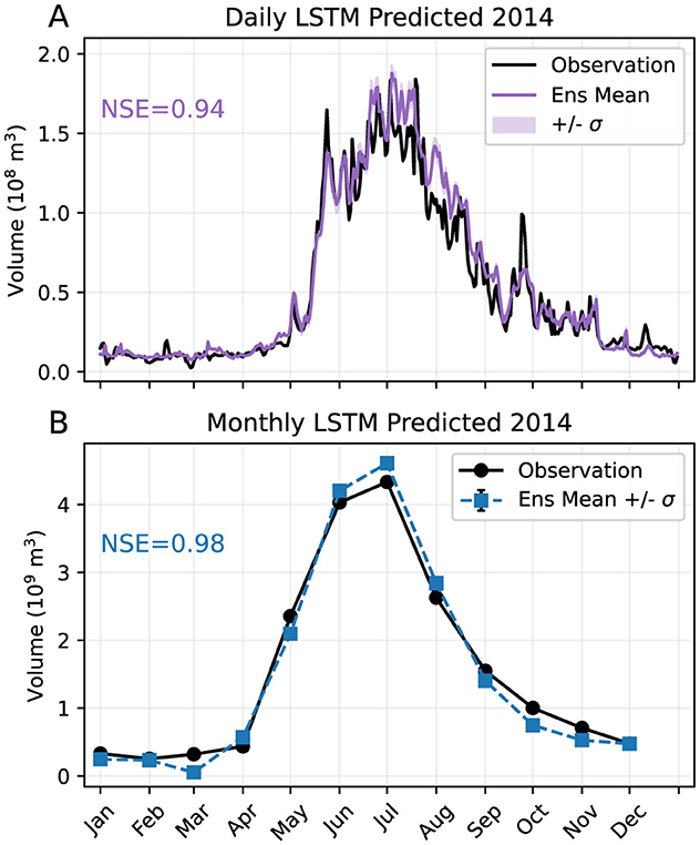
Figure 2. Observed and predicted streamflow for an example test year (2014) from (A) the daily LSTM model and (B) the monthly LSTM model with n = 12 months. The ensemble mean (Ens Mean) is the mean across the five models. Plus/minus one standard deviation (+/– σ) across the ensemble models is indicated by shading in (A) and error bars in (B). Note that standard deviations are small and not visible in (B). Observed streamflow is indicated by the black curves. The NSE values of the ensemble means are printed in each plot area.

The total seasonal volumes calculated from the daily and monthly LSTM outputs are compared to observed total seasonal volumes (Figure 3). For the daily model (Figure 3a), some test years have large standard deviations across the ensemble members, shown in the error bars. The model overestimates seasonal volumes in all years with low volumes (< 1.5 × 10¹⁰ m³) and underestimates seasonal volumes in all years with high volumes (>1.8 × 10¹⁰ m³). This results in a negative R² of –0.56 and a r almost zero (1.7 × 10⁻³) with p>0.05, reflecting the model's poor ability to capture interannual variability in seasonal volumes.

Figure 3

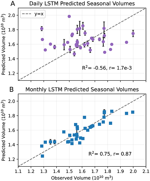
Figure 3. Predicted total seasonal (January to September) volumes with (A) the daily LSTM model and (B) the monthly LSTM model with n = 12 months, vs. observed seasonal volumes for test years in the range 1982–2017. Each point indicates the volume of the ensemble mean, and error bars indicate plus/minus one standard deviation across the ensemble models. R² and r values are printed in the plot areas. The dashed gray line indicates y = x.

The monthly model with n = 12 months (Figure 3b) captures the interannual variability in seasonal volumes more accurately than the daily model. The variance across the ensemble members is also lower, with standard deviation error bars visible only for a few years. The R² of 0.75 and r of 0.87 with p < 0.05 indicating statistical significance reflects much better predictive skill of total seasonal streamflow anomalies (i.e. relative to the climatology) compared to the daily model. The results for the model runs with n = 24 and 36 are similar to those of n = 12, with R² of 0.70 and r of 0.85 for n = 24, and R² of 0.71 and r of 0.86 for n = 36 (not shown). Completing five sets of n = 12 model runs, where each set differs only in the random order of training and validation years, gives mean R² and r of 0.74 and 0.86, with standard deviations 0.02 and 0.01, respectively (Table 1). This suggests that the high skill seen with the n = 12 model is robust to changes in the order of training and validation data. All further analysis is thus completed with the 12-month model.

Table 1

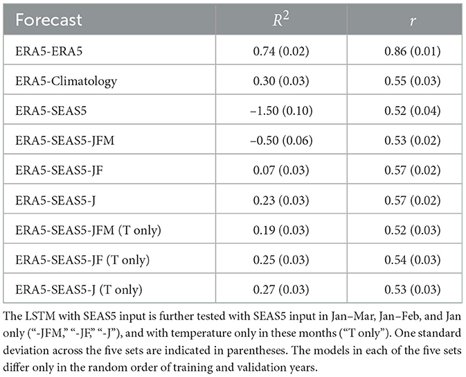
Table 1. Mean R² and r across five sets of 36 models testing on 36 test years for the LSTM trained on ERA5 with ERA5 input (“ERA5-ERA5”), with ERA5 climatology input (“ERA5-Climatology”) and with SEAS5 input (“ERA5-SEAS5”).

Previous studies have found that models with multiple LSTM layers perform better than those with a single LSTM layer, with many studies choosing two-layer LSTM models (Kratzert et al., 2018; Hauswirth et al., 2021; Zheng et al., 2024). To test whether this is the case for the Mica catchment, an additional LSTM layer is added into our model. A dropout layer is inserted between the two LSTM layers, following Kratzert et al. (2018), to prevent overfitting. This two-layer LSTM model does not perform better than the single-layer model reported above, in fact it obtains lower R² and r values of 0.41 and 0.70, respectively. This indicates that adding an additional LSTM layer to the model does not increase model performance. The single-layer LSTM model is used in all further analysis.

We compare our results to those calculated from the LSTM models applied to multiple streamflow stations across Western Canada (Anderson and Radić, 2022) and the United States (Kratzert et al., 2019) in Figure 4. Anderson and Radić (2022) employ a convolutional neural network (CNN) combined with an LSTM to predict daily streamflow of 226 stations across British Columbia and Alberta. We use their published model outputs to generate streamflow curves and calculate total seasonal volumes for their five test years (2011–2015) for comparison to our simulation. Kratzert et al. (2019) develop a daily LSTM to predict streamflow at 531 stations across the United States. We use the published results from one of their models without static catchment attributes to calculate seasonal volumes of their ten test years (1990–1999). We select their stations with NSE >0 and R²>−1.0 to better visualize the results (43 stations from Anderson and Radić, 2022 and 472 stations from Kratzert et al., 2019). The evaluation metrics calculated for our station are not outliers from the distribution of values from these two studies, although our station's NSE is among the stations with highest NSE, and the daily model is unusual in having such a low r with such a high NSE. Our daily model has the lowest r but not the lowest R² and our monthly model does not have the highest R² or r. The high NSE of our basin is likely related to the strong seasonality of the streamflow.

Figure 4

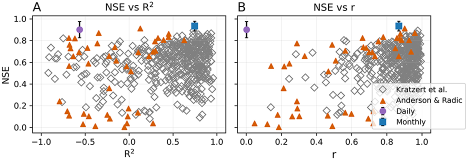
Figure 4. Performance of our daily and 12-month LSTM models compared to those of Kratzert et al. (2019) and Anderson and Radić (2022). For each station modeled by Kratzert et al. (2019) and Anderson and Radić (2022), the NSE calculated across their test years (10 and 5 years, respectively) is plotted against (A) R² and (B) r calculated from the seasonal volumes of their test years. Only stations with NSE >0 and R²>−1.0 are plotted (472 and 43 stations, respectively). The mean NSE across five sets of model runs for our daily and monthly models are plotted against the mean R² and r across all five sets of model runs. Error bars indicate plus/minus one standard deviation across the five sets of model runs.

The higher temporal resolution with the daily model allows the user to identify local daily extremes in streamflow, which is lost with the monthly timescale; however, the monthly model is better able to predict interannual variability in seasonal volume, which is the focus of the current study. The monthly LSTM model is therefore used for all further analysis.

Previous studies on catchments in the United States have shown that LSTM models trained on multiple catchments can perform better than those trained on a single catchment (Kratzert et al., 2018, 2019, 2024). These studies suggest a larger training dataset that spans multiple catchment types of streamflow responses enables the LSTM model to ‘fine tune' the learning of relationships between forcings and streamflow. To test the impact of this for our study, we repeat our analysis on an LSTM model trained on 265 stations across British Columbia and Alberta from Environment and Climate Change Canada's Historical Hydrometric Data website (similar to Anderson and Radić, 2022), and fine-tuned on the Mica catchment. This multi-basin method gave similar results for the monthly LSTM model, with R² of 0.60 and r of 0.80 for n = 12 (not shown), suggesting there is no advantage to training on multiple catchments when predicting seasonal volumes for the Mica catchment.

3.2 Seasonal streamflow sensitivity to meteorological lead time skill

Having established that the monthly LSTM model predicts interannual streamflow variability with good skill using observed (ERA5) meteorological data, we explore how much lead time in meteorological forecast skill is needed for an accurate total seasonal streamflow forecast. We use a combination of ERA5 reanalysis (i.e. “perfect” meteorological skill) and climatology (i.e. no meteorological skill) data to simulate different levels of forecast skill for each test year.

Since we are using the 12-month model, the first 12 minus i months use ERA5 data (past year), while the remaining i months use either ERA5 or climatology data to represent varying meteorological forecast skill. For example, to test for the importance of meteorological skill in January and February of the forecast year, ERA5 data are used for the first two months of the year, and climatological values are used for the remaining months. Figure 5 presents a schematic of the inputs used in this example.

Figure 5

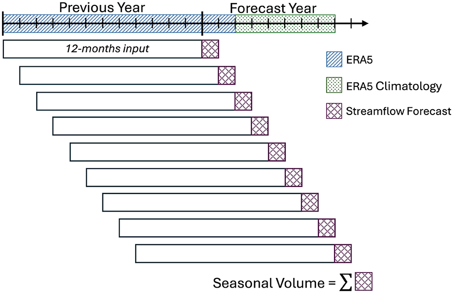
Figure 5. Schematic showing forcings input into the pre-trained LSTM model for a simulation of meteorological skill in January and February of the forecast year only. ERA5 reanalysis is used in months with meteorological skill and ERA5 climatology is used in months with no meteorological skill.

Nine simulations of different levels of meteorological skill are completed (Figure 6). The results show that good streamflow skill (R² = 0.73) is achievable with meteorological skill extending just three months into the forecast year (Jan–Mar). Note that although the simulation with meteorological skill in Jan-Apr achieves a slightly higher R² than the simulation with meteorological skill in all months (“All” in Figure 6), the means are not significantly different (p>0.1 in a Student's t-test), and thus we cannot reject the null hypothesis that the two means are equal. Extending forecast skill beyond this period adds minimal improvement, indicating that accurate seasonal forecasts mainly depend on meteorological data up to three months into the forecast year. Conversely, when meteorological skill is applied only in late spring and summer (May–Aug), no significant improvement in streamflow forecasting is observed, highlighting the critical importance of winter snowpack accumulation for seasonal streamflow volume in this basin.

Figure 6

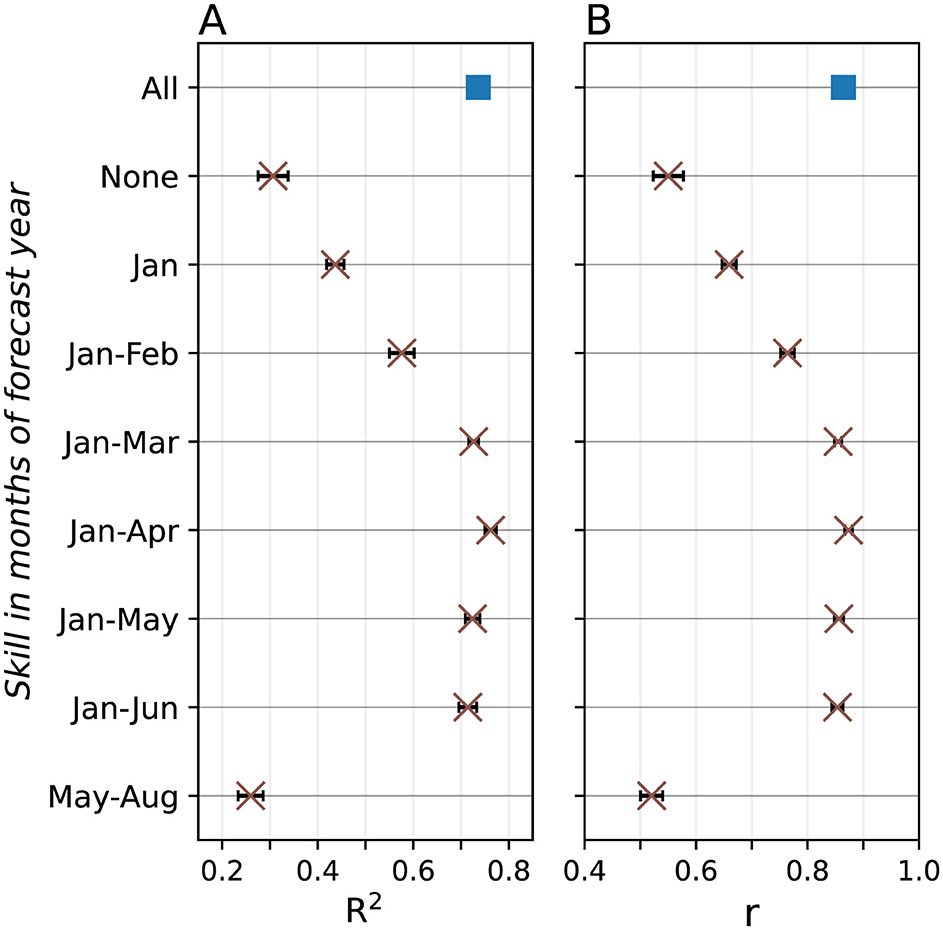
Figure 6. The (A) R² and (B) r calculated from the seasonal volumes of nine simulations of various levels of skill in input forcings. Error bars indicate plus/minus one standard deviation across five sets of model runs. Months of the forecast year with meteorological skill use ERA5 reanalysis forcings, while months without meteorological skill use monthly ERA5 climatological forcings.

3.3 Hybrid streamflow forecasts

Our hybrid streamflow forecasts use SEAS5 hindcast data as meteorological input for the “future” months. To first understand the meteorological skill, and any biases, of the SEAS5 dataset, values of Tmin, Tmax, and Precip averaged over the Mica catchment area are compared to ERA5 for lead times 1–3 months (Figure 7). The hindcasts underestimate Tmin relative to ERA5 in almost all years at all three lead times. Tmax is underestimated in almost all years for lead time 1 month, and in just over half of years for lead times 2 and 3 months. However, the hindcasts exhibit significant linear relationships with ERA5 (p < 0.05) out to 3 months lead for Tmin and 5 months lead (not shown) for Tmax. As expected, precipitation hindcasts do not perform as well, with a significant linear relationship (p < 0.05) only for 1 month lead. Precipitation is underestimated in many years, particularly at 3 months lead time. The results of Section 3.2 suggest that skill in the input meteorological forcings is required only out to ~3 months lead time for a skillful seasonal volume forecast. Thus, we judge that the significant skill in the SEAS5 hindcasts in these initial months, particularly in temperature, may be sufficient to provide some skill in the hybrid statistical-dynamical seasonal volume forecast.

Figure 7

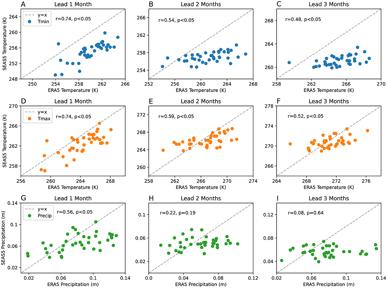
Figure 7. SEAS5 hindcasts of (A–C) minimum temperature (Tmin), (D–F) maximum temperature (Tmax), and (G–I) precipitation (Precip) vs. ERA5 reanalysis of 1981–2017. The hindcasts are initialized 1 January and lead times 1, 2, and 3 months are presented, showing forecasts for January, February, and March, respectively. Pearson correlation r-values and p-values are printed in each plot area. The dashed gray lines indicate y = x.

Similar to the method of Section 3.2, the first 12 minus i months of the hybrid forecast inputs use ERA5 forcings (past year). The following i months in the forecast year use SEAS5 hindcast data. As SEAS5 hindcasts extend to only 6 months lead time, we can only use SEAS5 hindcast data for January to June. For forecasts of August and September streamflow, the remaining months of forcings (July and August) use ERA5 climatology. Figure 8 presents a schematic of the inputs used to predict seasonal volume of one test year. We refer to this hybrid forecast as ERA5-SEAS5, using the naming convention of the training dataset (ERA5) followed by the input dataset (SEAS5); we use the same naming convention for all hybrid forecasts.

Figure 8

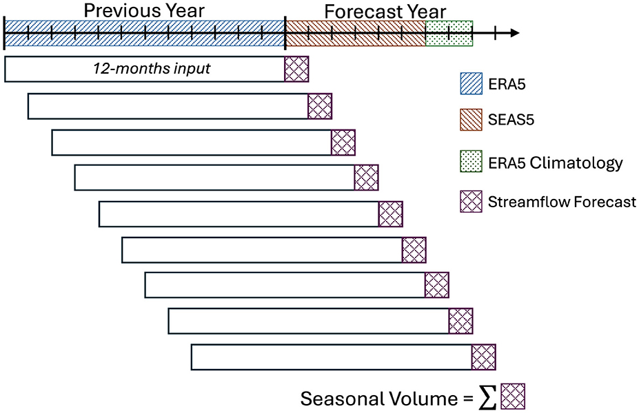
Figure 8. Schematic showing forcings input into the pre-trained LSTM model for the hybrid ERA5-SEAS5 streamflow forecast.

The hybrid ERA5-SEAS5 streamflow forecast for one test year (2014) is presented in Figure 9a, with observed monthly volumes and the results of the LSTM with ERA5 input (denoted “ERA5-ERA5,” also shown in Figure 2b). The hybrid ERA5-SEAS5 forecast predicts lower monthly volumes than the ERA5-ERA5 forecast for all months January to September. This translates into a lower seasonal volume prediction. The ERA5-SEAS5 forecast underestimates seasonal volumes for almost all of the 36 test years (Figure 9b). This is reflected in the negative R² of –1.53. However, the r of 0.48 indicates there is a linear relationship between the hybrid-forecasted volumes and observed seasonal volumes, and the ERA5-SEAS5 forecast correctly predicts some of the interannual variability in seasonal volumes. A bias correction step in post-processing of the forecast results could correct the climatological volume underestimation. Repeating four additional sets of model runs, where each run differs only in the order of training and validation data, yields a mean R² and r of −1.50 and 0.52 with standard deviations 0.10 and 0.04, respectively (Table 1). The high standard deviation of the R² indicates there is some disagreement among model runs, however the r values are more consistent.

Figure 9

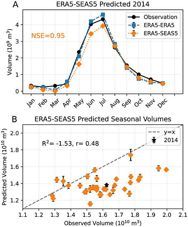
Figure 9. (A) Observed and modeled monthly volumes for one example test year (2014) with predicted volumes from the ERA5-SEAS5 forecast (orange diamonds), predicted volumes from the LSTM with ERA5 input (“ERA5-ERA5”; blue squares), and observed volumes (black circles). The NSE value of the ERA5-SEAS5 forecast is printed in the plot area. (B) Seasonal (Jan–Sep) volumes predicted by the ERA5-SEAS5 forecast vs. observed seasonal volumes for the test years 1982–2017. The R² and r values are printed in the plot area. The seasonal volume of 2014 is plotted as a black star, and the dashed gray line indicates y = x. Both monthly volumes (A) and seasonal volumes (B) shown are ensemble means of five models, and error bars indicate plus/minus one standard deviation across the ensemble models.

The seasonal volume underestimation by the hybrid ERA5-SEAS5 forecast is physically consistent with an average underestimation of winter precipitation seen in Figures 7g–i, and of the underestimation of Tmin and Tmax during the summer (similar to winter/early spring shown in Figure 7). The lower hindcast Precip values in January, February, and March translate to less snowpack buildup, and the lower Tmin and Tmax values in April, May, and June result in less glacier and/or snowmelt.

Critically, the hybrid ERA5-SEAS5 streamflow forecast does not perform better than a forecast that uses meteorological climatology as input in all months of the forecast year, as seen in Section 3.2 (Figure 6, simulation labeled “None”). The forecast with climatology as input in all months, hereafter referred to as ERA5-Climatology to follow our naming convention, achieves a mean R² of 0.30 and mean r of 0.55, higher than the R² of the ERA5-SEAS5 forecast (–1.50), and not statistically different from the r value (0.52). This suggests that the underestimation of meteorological conditions in the SEAS5 hindcasts is critical in limiting the ability of the hybrid streamflow forecast to simulate the absolute streamflow volumes—using climatological meteorological conditions in the forecast year produces a forecast better able to capture the annual seasonal volume. Whilst the SEAS5 forecast can predict some of the interannual variability (as measured by r) of temperature with lead times of 1–3 months (as seen in Figure 7), this does not translate into any improved skill in predicting seasonal streamflow interannual variability.

The results of Section 3.2 suggest that, in this basin, only meteorological skill in the first three months of the forecast year is necessary to achieve skill in a seasonal volume forecast (when meteorological climatology are used for the remaining months). The skill of the SEAS5 hindcasts diminishes rapidly with lead time, and thus we investigate whether only using SEAS5 hindcast data in the early months of the forecast (with meteorological climatology in the latter months) improves the skill of the hybrid forecast. Table 1 presents mean R² and r achieved in a hybrid forecast with SEAS5 hindcasts used as input in Jan–Mar only and meteorological climatology used for the remaining months of the forecast year (“ERA5-SEAS5-JFM”), compared with mean R² and r of ERA5-ERA5, ERA5-Climatology, and ERA5-SEAS5. The R² of ERA5-SEAS5-JFM forecast is still negative, however there has been a significant improvement compared to ERA5-SEAS5. Replacing another month with meteorological climatology input (SEAS5 input Jan–Feb only; “ERA5-SEAS5-JF”) further improves the R² values, and slightly improves the r value (from 0.53 to 0.57). A forecast with SEAS5 input in January only (“ERA5-SEAS5-J”) achieves the highest R² of 0.23, however this is still significantly lower than the ERA5-Climatology forecast, and the highest r is within the uncertainty range of the r value of the ERA5-Climatology forecast. This suggests that there is no added skill in using SEAS5 hindcasts of Tmin, Tmax, and Precip as input for future months in a hybrid forecast, relative to using climatological values for the future months.

Lastly, we investigate the roles of precipitation and temperature separately. As seen in Figure 7, SEAS5 Precip hindcasts exhibit a significant linear relationship with ERA5 only for a lead time of 1 month. Including SEAS5 Precip in the ERA5-SEAS5-JFM and ERA5-SEAS5-JF forecasts likely introduces bias and uncertainty that translates into errors in the streamflow forecast. Using climatological values for Precip in all months, whilst still using SEAS5 hindcasts for Tmin and Tmax in Jan–Mar (with climatology for the remaining months), improves the mean R² from –0.50 to 0.19 (“ERA5-SEAS5-JFM (T only)” in Table 1), illustrating the important role of precipitation biases and uncertainty in forecast error. These results, summarized in Table 1, indicate that the inclusion of SEAS5 Precip does not contribute any significant skill to the streamflow forecast. Forecasts with SEAS5 data in January only (whether including Precip or not), and climatology for the remaining months in the forecast year (“ERA5-SEAS5-J” and “ERA5-SEAS5-J (T only)”) achieve the highest skill when considering both R² and r. Neither of these forecasts provide any statistically significant improvement from a forecast using climatological meteorology in the forecast year.

In the next section, we test methods of bias correcting the SEAS5 inputs to determine whether this can reduce the bias in seasonal streamflow of the hybrid forecast, and provide any additional skill.

3.3.1 Streamflow forecast with bias-corrected input data

Our first bias correction method linearly shifts the SEAS5 hindcasts to obtain the same mean as ERA5 in each month. These linearly shifted hindcasts (SEAS5-LS) are then used as forecast year input to the LSTM trained on ERA5, similar to the ERA5-SEAS5 input in Figure 8. We denote this linearly shifted hybrid forecast ERA5-SEAS5-LS. Figure 10a presents the hybrid ERA5-SEAS5-LS predicted streamflow forecast for one test year (2014), with observed monthly volumes and ERA5-ERA5 results. The ERA5-SEAS5-LS forecast predicts higher volumes for the first seven months compared to the ERA5-SEAS5 forecast in Figure 9a, thus a higher seasonal volume for 2014 is predicted (Figure 10b), although the seasonal volume is still underestimated by a small amount. Overall, the underestimation of seasonal volumes is reduced in ERA5-SEAS5-LS (Figure 10b) compared to the ERA5-SEAS5 forecast (Figure 9b), leading to a positive R² of 0.28. The r of 0.56 is also higher than that of the ERA5-SEAS5 forecast (0.48), indicating there is an improvement in predicting interannual variability of seasonal volumes with the linearly shifted SEAS5 inputs. Completing five sets of model runs gives mean R² and r of 0.24 and 0.54, with standard deviations 0.04 and 0.03, respectively (summarized in Table 2).

Figure 10

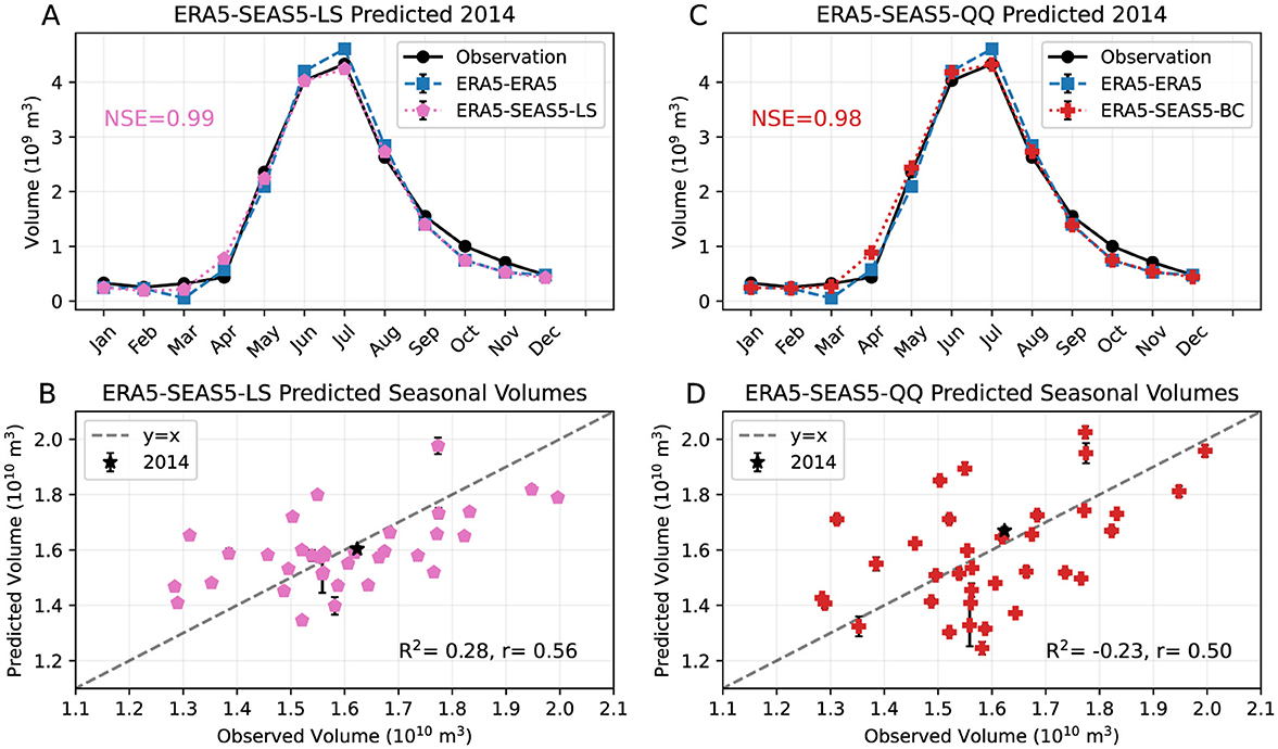
Figure 10. (A) Observed and modeled monthly volumes for one example test year (2014) with predicted volumes from ERA5-SEAS5-LS (pink pentagons), predicted volumes ERA5-ERA5 (blue squares), and observed volumes (black circles). The NSE value of the ERA5-SEAS5-LS forecast is printed in the plot area. (B) Seasonal (Jan–Sep) volumes predicted by the ERA5-SEAS5-LS forecast vs. observed seasonal volumes for the test years 1982–2017. The R² and r values are printed in the plot area. The seasonal volume of 2014 is plotted as a black star, and the dashed gray line indicates y = x. (C) As (A) but for predicted volumes from ERA5-SEAS5-QQ (red crosses). (D) As (B) but for seasonal volumes predicted by the ERA5-SEAS5-QQ forecast. Both monthly volumes (A, C) and seasonal volumes (B, D) shown are ensemble means of five models, and error bars indicate plus/minus one standard deviation across the ensemble models.

Table 2

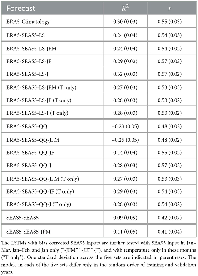
Table 2. Mean R² and r across five sets of 36 models testing on 36 test years for the LSTM trained on ERA5 with ERA5 climatology input (“ERA5-Climatology,” as in Table 1), with shifted SEAS5 input (“ERA5-SEAS5-LS”), with quantile–quantile bias corrected SEAS5 input (“ERA5-SEAS5-QQ”), and the LSTM trained on SEAS5 with 6 months of SEAS5 input (“SEAS5-SEAS5”) and 3 months of SEAS5 input (“SEAS5-SEAS5-JFM”).

The ERA5-SEAS5-LS forecast still does not provide any significant improvement on the forecast with meteorological climatology input in all months of the forecast year, ERA5-Climatology, with R² and r of 0.30 and 0.55 respectively. Table 2 presents mean R² and r values from forecasts that use SEAS5-LS as input in Jan–Mar only (“ERA5-SEAS5-LS-JFM”), Jan–Feb only (“ERA5-SEAS5-LS-JF”), and January only (“ERA5-SEAS5-LS-J”) in the forecast year, with meteorological climatology used in the remaining months. Whilst the mean R² improves with only using SEAS5-LS in January of the forecast year, which was also seen in the previous section with the forecasts without bias-correction on the input data (see Table 1), it is still not significantly different from the ERA5-Climatology forecast. This is also true for a hybrid forecast using linearly shifted SEAS5 data of temperature only, with climatological Precip—see data for ERA5-SEAS5-LS-JFM, -JF, and -J (T only) in Table 2.

We next use a quantile–quantile (QQ) bias correction method to allow for correction of non-linear biases (e.g. if high values are underestimated more than low values, as seen for lead months 2 and 3 in Figure 7). These bias corrected hindcasts (SEAS5-QQ) are then used as forecast year input to the LSTM trained on ERA5, and we denote this bias corrected hybrid forecast ERA5-SEAS5-QQ. Note that for this method to be applicable in operational settings, a formula to apply the quantile–quantile bias correction to future years would need to be derived. The monthly volumes predicted by the ERA5-SEAS5-QQ forecast for one test year (2014) are presented in Figure 10c, with observed monthly volumes and the ERA5-ERA5 results. Compared to the ERA5-SEAS5 forecast in Figure 9a, the ERA5-SEAS5-QQ forecast gives a higher prediction of seasonal volume for 2014 (Figure 10d), slightly over the observed seasonal volume of that year. The average bias in streamflow over all years is small (Figure 10d) compared to the ERA5-SEAS5 forecast (Figure 9b). Completing five sets of model runs results in a mean R² of –0.23, and r of 0.48, higher than the uncorrected ERA5-SEAS5 model, but lower than the ERA5-SEAS5-LS forecast and the ERA5-Climatology (Table 2).

As with the previous bias correction method, we investigate the impact of using SEAS5-QQ hindcasts as input in Jan–Mar, Jan–Feb, and Jan only in the forecast year, and of using climatological Precip in all months. These results are summarized in Table 2, denoted “ERA5-SEAS5-QQ-JFM” etc. Similar to the results for the LS bias correction method, reducing the number of months (and thus the lead time) of the SEAS5 forecast data increases the R² and r values, but overall the skill in the QQ forecasts is typically lower than that of the corresponding LS method, and no configuration significantly improves on the ERA5-Climatology forecast.

3.3.2 Streamflow forecast with re-trained LSTM model

As shown in the previous section, bias correcting the seasonal meteorological forecast data input into the hybrid forecast yields little to no improvement to the model's ability to predict the interannual variations in seasonal streamflow, as measured by r, and no hybrid forecast was able to improve upon a forecast that uses meteorological climatology in all months of the forecast year. Here, we investigate whether the model skill can be improved if the LSTM model is trained on the seasonal meteorological forecasts in the forecast year instead of ERA5 (ERA5 is still used in the past year). In this way, the model can indirectly learn and “correct” for the biases present in the seasonal forecast. For every forecast year within the training, validation, and testing datasets, we apply the same set-up for the 12 months of forcings as in the ERA5-SEAS5 forecast in Figure 8, i.e. ERA5 in the previous year, SEAS5 in the first 6 months in the forecast year, and meteorological climatology in the remaining months in the forecast year; this forecast is denoted SEAS5-SEAS5.

The monthly streamflow volumes predicted by the SEAS5-SEAS5 forecast for one test year (2014) are presented in Figure 11a, with observed monthly volumes and the ERA5-ERA5 results. This SEAS5-SEAS5 forecast generally predicts higher volumes than the ERA5-SEAS5 forecast (Figure 9a), indicating the model is able to correct for the low temperature and precipitation bias present in the hindcasts. The seasonal volume prediction for this year is still underestimated compared to observations (Figure 11b), but by less than the ERA5-SEAS5 forecast in Figure 9b. Overall, the underestimation bias seen in ERA5-SEAS5 is reduced, with the SEAS5-SEAS5 achieving an R² of 0.17 (Figure 11b). Completing five sets of model runs gives a mean R² of 0.09, and a mean r of 0.42 (Table 2), similar to the ERA5-SEAS5 and ERA5-SEAS5-QQ mean r values, and lower than both the ERA5-SEAS5-LS forecast, and the ERA5-Climatology.

Figure 11

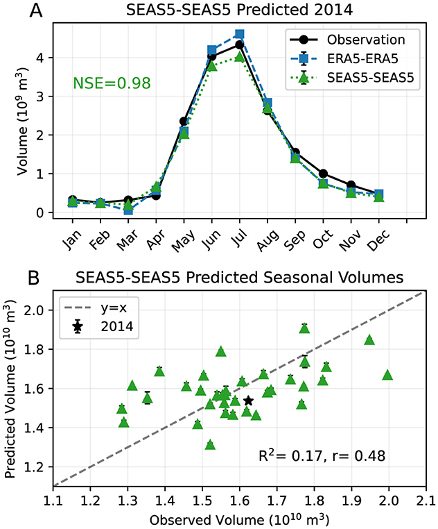
Figure 11. (A) Observed and modeled monthly volumes for one example test year (2014) with predicted volumes from SEAS5-SEAS5 (green triangles), predicted volumes ERA5-ERA5 (blue squares), and observed volumes (black circles). The NSE value of the SEAS5-SEAS5 forecast is printed in the plot area. (B) Seasonal (Jan–Sep) volumes predicted by the SEAS5-SEAS5 forecast vs. observed seasonal volumes for the test years 1982–2017. The R² and r values are printed in the plot area. The seasonal volume of 2014 is plotted as a black star, and the dashed gray line indicates y = x. Both monthly volumes (A) and seasonal volumes (B) shown are ensemble means of five models, and error bars indicate plus/minus one standard deviation across the ensemble models.

Following from the results of Section 3.3, where the hybrid forecasts perform worse when SEAS5 hindcasts are included as input beyond three months of the forecast year, we train an LSTM model on SEAS5 hindcasts in Jan–Mar and ERA5 for the remaining months. This trained model, denoted SEAS5-SEAS5-JFM is then tested with SEAS5 data in Jan–Mar in the forecast year and meteorological climatology for the remaining months. This SEAS5-SEAS5-JFM forecast performs about the same as SEAS5-SEAS5, with mean R² of 0.11 and mean r of 0.41, both within one standard deviation of the means of SEAS5-SEAS5. Thus, training the LSTM on fewer months of SEAS5 hindcasts does not result in any improvement in skill. Both the SEAS5-SEAS5 and SEAS5-SEAS5-JFM forecasts have mean R² significantly lower than the ERA5-Climatology forecast, indicating these forecasts do not improve upon using meteorological climatology input into the LSTM trained on ERA5 for all months in the forecast year.

4 Discussion

Out of the four hybrid forecast types we test in this work, ERA5-SEAS5, ERA5-SEAS5-LS, ERA5-SEAS5-QQ, and SEAS5-SEAS5, the ERA5-SEAS5-LS forecast obtains the highest mean R² value (0.24) across five sets of model runs (see Table 2), indicating that the linear bias correction method provides the greatest skill in predicting climatological mean seasonal volumes. The SEAS5-SEAS5 forecast obtains a positive R² value, but significantly lower than that of the ERA5-SEAS5-LS forecast, indicating it is more effective to input bias-corrected data to the LSTM model rather than train the LSTM model on the SEAS5 hindcasts.

The ERA5-SEAS5-LS forecast also obtains the highest r value (mean 0.54); however, this is not a large improvement on the other hybrid forecasts ERA5-SEAS5 and ERA5-SEAS5-QQ, each with similar mean r values (0.48–0.52). Thus, bias correction of the meteorology SEAS5 inputs does not substantially improve the skill in predicting interannual variability in seasonal volumes. The SEAS5-SEAS5 forecast has a lower mean r value (0.42). Thus, attempting to correct for systematic biases in the SEAS5 by training forecasts on the SEAS5 hindcasts is not as effective at improving the skill as applying a simple linear shift correction to SEAS5 data prior to using it as input. Whilst the SEAS5-SEAS5 model does likely learn to correct for systematic biases in the SEAS5 hindcasts, it is probable that the uncertainty in the SEAS5 hindcasts prevent the model from learning the true relationships between temperature, precipitation and seasonal mean streamflow.

Of note, none of our hybrid forecasts exhibit significantly higher skill than a forecast that uses meteorological climatological inputs to the LSTM model for each month in the forecast year (ERA5-Climatology). The ERA5-Climatology forecast derives its skill from the previous year's meteorological conditions. This is consistent with physical knowledge of this basin, in which snowpack is known to be a key factor in subsequent streamflow. Using fewer months of SEAS5 input (i.e. only forecasts with shorter lead times) and replacing longer lead time input with meteorological climatology improves forecasts trained on ERA5 data, with the ERA5-SEAS5-LS-JF, ERA5-SEAS5-LS-J, and the ERA5-SEAS5-QQ-J forecasts giving the highest mean R² and r values of the hybrid SEAS5 forecasts. This indicates that skill can be improved by limiting the use of SEAS5 data to shorter lead times, even when using bias correction techniques. While these models all have slightly higher mean r (0.57) relative to the ERA5-Climatology forecast (0.55), the difference is very small—there is thus still little to no added skill in using SEAS5 input rather than meteorological climatology. This suggests that the skill of the SEAS5 meteorological forecasts in lead months 1–3 is insufficient to translate to any substantial increase in skill in the hybrid seasonal streamflow forecasts.

Since precipitation hindcasts exhibit more biases and less correlation with ERA5, using only SEAS5 temperature hindcasts and climatological precipitation further improve the forecasts. Both the ERA5-SEAS5-LS-JFM and ERA5-SEAS5-QQ-JFM forecasts with SEAS5 temperature in Jan–Mar only and climatological precipitation in all months obtain mean R² values within one standard deviation of the ERA5-Climatology forecast, an improvement upon their equivalents that use SEAS5 precipitation in Jan–Mar. There is no improvement in further reducing the number of months that use SEAS5 temperature input; the forecasts with SEAS5 temperature input in Jan–Mar, Jan–Feb, and Jan only for both bias correction techniques all obtain R² values within 0.01 of each other.

The SEAS5 hindcasts will likely continue to improve in the future as advances are made to the forecast model. These future changes may improve upon the bias and uncertainty in the meteorological variables in the Mica catchment area. It will be necessary to continue to evaluate whether hybrid forecasts can improve on forecasts with ERA5 climatology in the forecast year for this region. Other methods to obtain meteorological forecasts at least three months into the future, such as statistical techniques, may also be useful, rather than relying on numerical forecasts. Hsieh et al. (2003) use multiple linear regression (MLR) to predict seasonal April–August streamflow further downstream in the Columbia River basin using modes of climate variability indices. They find a range of r values from 0.47–0.70 for various predictor combinations. The hybrid forecasts in our study perform similarly to this MLR based on r values, suggesting that using a statistical technique such as MLR may be able to provide improved streamflow forecasts, and this is worth investigating in future work.

The forecasts developed in this study use a simple LSTM model with one layer. Increasing the number of LSTM layers from one to two did not improve results, however there are other parameters of the LSTM model that can be varied and may improve model performance, such as the length of the hidden and cell state vectors and the loss function used. Kratzert et al. (2019) found the inclusion of static catchment attributes, including area, mean elevation, and fraction of snow, improved LSTM model performance. As the Mica catchment is in a mountainous area, the model may benefit from a snowpack measure that facilitates the relationship between temperature, precipitation, and snowmelt. Other studies, such as Tang et al. (2024), suggest that segmenting training data into dry and wet periods and training separate models for each characteristic may improve model performance; the strong seasonal streamflow variations in our basin indicate this technique may be useful. Modifications to the LSTM model architecture, such as those suggested above, could improve the benchmark performance of the LSTM model, i.e. with ERA5 input (ERA5-ERA5). LSTM forecasts would likely also improve; however, this may not lead to any improvement of the hybrid forecasts relative to ERA5-Climatology. Future studies will need to assess whether there is substantial improvement to the hybrid forecasts with LSTM architecture modification beyond that of ERA5-Climatology.

Due to the limitations from meteorological input on the hybrid forecast skill, other types of forecast model may show improvement beyond that of the hybrid statistical-dynamical forecast, for example, combining LSTM models with other deep learning methods or streamflow forecasts. Zheng et al. (2024) use a Bayesian deep learning approach with an LSTM to improve quantification of uncertainty, and Modi et al. (2025) combine an LSTM with a probabilistic ensemble streamflow prediction forecast. In addition, Modi et al. (2025) found their models that included past snow accumulation performed better than those without, further highlighting that a snowpack measure may be useful.

We note that our results are for a snowmelt-dominated catchment with low streamflow levels in the winter and high levels in the spring and summer, and this likely has a strong impact on some of our conclusions, particularly on the forecast skill that can be acquired with only Jan–Mar meteorological data (see Figure 6), as the snowmelt accumulated during September to March plays a substantial role in summer streamflow. Further work is required to understand which of our results can be generalized to other basins.

5 Summary and conclusions

This study develops and analyzes the performance of a hybrid statistical-dynamical streamflow model for seasonal forecasting of total January to September inflow volume at 9 months lead time, i.e. at the beginning of January. We focus on a single catchment that flows into the Kinbasket Lake Reservoir and Mica Dam in southeast British Columbia, a snowmelt-dominated catchment with low streamflow levels in the winter and high levels in the spring and summer. The hybrid forecast uses dynamical seasonal meteorological hindcasts from ECMWF SEAS5 as input into an LSTM model trained on meteorological forcings and streamflow observations. We use a leave-1-year-out cross validation methodology, performing 36 model runs in total, each tested on a different year in 1982–2017 and trained and validated on a random selection of the remaining 35 years. We summarize the major findings of this study as follows:

1. The monthly LSTM model, which uses the previous 12 months of meteorological data, outperforms the daily model (using the previous 365 days) in capturing seasonal volumes and their interannual variability, achieving an R²>0.7, while the daily model fails to capture this variability effectively (R² < 0).

2. For this catchment, only 3 months of accurate meteorological input (January–March) are needed to achieve high predictive skill for seasonal streamflow, with little to no added value from meteorological skill in the summer months (May–August).

3. The hybrid forecast (ERA5-SEAS5) tends to underestimate streamflow volumes due to biases in the SEAS5 hindcasts. Despite this, the model captures over half of the interannual variability (r≈0.52).

4. Applying linear and quantile–quantile bias corrections to the SEAS5 hindcasts improves the accuracy of seasonal volume predictions but does not significantly enhance the model's ability to predict interannual variability.

5. Training the LSTM model directly on SEAS5 data enables better volume predictions but slightly reduces the model's skill in capturing interannual variability (r≈0.42).

6. Reducing the number of months of SEAS5 hindcasts input improves the forecasts, as the hindcast data with significant biases relative to ERA5 are removed.

7. No hybrid forecast is able to substantially improve upon a forecast with meteorological climatology input in all months of the forecast year (mean R² = 0.30, r = 0.55), indicating that there is currently little to no added value in using SEAS5 forecast input.

The results presented demonstrate that although it is possible to use a hybrid statistical-dynamical LSTM forecast to predict seasonal volumes with 9 months lead time, there is no added skill in using SEAS5 hindcast data as input to the LSTM model for the forecast year compared to using meteorological climatology. However, some hybrid forecasts are able to reproduce the same skill level as the forecast with meteorological climatology input, and thus, as improvements are made to seasonal meteorological forecasts, there is the potential that these hybrid forecasts will provide improved predictions of seasonal volumes.

As our hybrid models use ERA5 reanalysis and ECMWF SEAS5 seasonal forecasts, both of which are available as global gridded datasets, our model framework could be applied to other catchments with streamflow observations available. Many of our results, particularly on the meteorological forecast months required for accurate seasonal streamflow predictions, are likely unique to snowmelt-dominated catchments; however, this framework is modifiable to use different predictor variables as input to better reflect streamflow processes in other regions.

Data availability statement

Publicly available datasets were analyzed in this study. ERA5 reanalysis data is available from the European Centre for Medium-Range Weather Forecasts (ECMWF) (Hersbach et al., 2020; https://cds.climate.copernicus.eu/datasets/reanalysis-era5-single-levels?tab=overviewECMWF). SEAS5 data is available from ECMWF (Johnson et al., 2019; https://cds.climate.copernicus.eu/datasets/seasonal-monthly-single-levels?tab=overview). Streamflow data is available from the Bonneville Power Administration (Dakhlalla et al., 2020; https://www.bpa.gov/energy-and-services/power/historical-streamflow-data). Code to reproduce all figures and results is available on Github (Swift-LaPointe, 2025; https://doi.org/10.5281/zenodo.15483232).

Author contributions

TS-L: Conceptualization, Formal analysis, Methodology, Visualization, Writing – original draft, Writing – review & editing. RW: Conceptualization, Methodology, Supervision, Writing – original draft, Writing – review & editing. VR: Conceptualization, Methodology, Supervision, Writing – original draft, Writing – review & editing.

Funding

The author(s) declare that financial support was received for the research and/or publication of this article. TS-L has been supported by a Natural Sciences and Engineering Research Council of Canada (NSERC) Discovery Grant (RGPIN-2020-05783), and a Mitacs Accelerate grant partnered with BC Hydro.

Acknowledgments

We wish to thank Greg West and Adam Gobena for their support and feedback throughout the project, and the anonymous reviewers for their comments that improved the work. We additionally wish to acknowledge that this work was completed through the use of computing resources at the University of British Columbia and Google Colab.

Conflict of interest

The authors declare that the research was conducted in the absence of any commercial or financial relationships that could be construed as a potential conflict of interest.

Generative AI statement

The author(s) declare that no Gen AI was used in the creation of this manuscript.

Publisher's note

All claims expressed in this article are solely those of the authors and do not necessarily represent those of their affiliated organizations, or those of the publisher, the editors and the reviewers. Any product that may be evaluated in this article, or claim that may be made by its manufacturer, is not guaranteed or endorsed by the publisher.

References

Abadi, M., Agarwal, A., Barham, P., Brevdo, E., Chen, Z., Citro, C., et al. (2015). TensorFlow: Large-scale Machine Learning on Heterogeneous Systems. Available online at: https://www.tensorflow.org/ (accessed July 3, 2024).

Google Scholar

Anderson, S., and Radić, V. (2022). Evaluation and interpretation of convolutional long short-term memory networks for regional hydrological modelling. Hydrol. Earth Syst. Sci. 26, 795–825. doi: 10.5194/hess-26-795-2022

Crossref Full Text | Google Scholar

Araya, D., Mendoza, P. A., noz Castro, E. M., and McPhee, J. (2023). Towards robust seasonal streamflow forecasts in mountainous catchments: impact of calibration metric selection in hydrological modeling. Hydrol. Earth Syst. Sci 27, 4385–4408. doi: 10.5194/hess-27-4385-2023

Crossref Full Text | Google Scholar

Arheimer, B., Pimentel, R., Isberg, K., Crochemore, L., Andersson, J. C. M., Hasan, A., et al. (2020). Global catchment modelling using World-Wide HYPE (WWH), open data, and stepwise parameter estimation. Hydrol. Earth Syst. Sci. 24, 535–559. doi: 10.5194/hess-24-535-2020

Crossref Full Text | Google Scholar

Arnal, L., Cloke, H. L., Stephens, E., Wetterhall, F., Prudhomme, C., Neumann, J., et al. (2018). Skilful seasonal forecasts of streamflow over Europe? Hydrol. Earth Syst. Sci. 22, 2057–2072. doi: 10.5194/hess-22-2057-2018

Crossref Full Text | Google Scholar

Chollet, F. (2015). Keras Github. Available online at: https://github.com/fchollet/keras (accessed July 3, 2024).

Google Scholar

Dakhlalla, A., Hughes, S., McManamon, A., Pytlak, E., Roth, T. R., van der Zweep, R., et al. (2020). 2020 Level Modified Streamflow: 1928-2018. Portland, OR: Bonneville Power Administration, Department of Energy.

Google Scholar

Day, G. N. (1985). Extended streamflow forecasting using NWSRFS. J. Water Resour. Plan. Manage. 111, 157–170. doi: 10.1061/(ASCE)0733-9496(1985)111:2(157)

Crossref Full Text | Google Scholar

Frame, J. M., Kratzert, F., Klotz, D., Gauch, M., Shalev, G., Gilon, O., et al. (2022). Deep learning rainfall–runoff predictions of extreme events. Hydrol. Earth Syst. Sci. 26, 3377–3392. doi: 10.5194/hess-26-3377-2022

Crossref Full Text | Google Scholar

Gobena, A. K., Weber, F. A., and Fleming, S. W. (2013). The role of large-scale climate modes in regional streamflow variability and implications for water supply forecasting: a case study of the Canadian Columbia river basin. Atmos. Ocean 51, 380–391. doi: 10.1080/07055900.2012.759899

Crossref Full Text | Google Scholar

Hamlet, A. F., Huppert, D., and Lettenmaier, D. P. (2002). Economic value of long-lead streamflow forecasts for Columbia River hydropower. J. Water Resour. Plan. Manage. 128, 91–101. doi: 10.1061/(ASCE)0733-9496(2002)128:2(91)

Crossref Full Text | Google Scholar

Hamlet, A. F., and Lettenmaier, D. P. (1999). Columbia River streamflow forecasting based on ENSO and PDO climate signals. J. Water Resour. Plan. Manage. 125, 333–341. doi: 10.1061/(ASCE)0733-9496(1999)125:6(333)

Crossref Full Text | Google Scholar

Hauswirth, S. M., Bierkens, M. F. P., Beijk, V., and Wanders, N. (2021). The potential of data driven approaches for quantifying hydrological extremes. Adv. Water Resour. 155:104017. doi: 10.1016/j.advwatres.2021.104017

PubMed Abstract | Crossref Full Text | Google Scholar

Hauswirth, S. M., Bierkens, M. F. P., Beijk, V., and Wanders, N. (2023). The suitability of a seasonal ensemble hybrid framework including data-driven approaches for hydrological forecasting. Hydrol. Earth Syst. Sci. 27, 501–517. doi: 10.5194/hess-27-501-2023

Crossref Full Text | Google Scholar

Hersbach, H., Bell, B., Berrisford, P., Hirahara, S., Horányi, A., noz-Sabater, J. M., et al. (2020). The ERA5 global reanalysis. Q. J. R. Meteorol. Soc. 146, 1999–2049. doi: 10.1002/qj.3803

Crossref Full Text | Google Scholar

Hills, K., Pruett, M., Rajagopalan, K., Adam, J., Liu, M., Nelson, R., et al. (2020). Calculation of 2020 irrigation depletions for 2020 Level Modified Streamflows. Washington, DC: Washington State University.

Google Scholar

Hsieh, W. W., and Tang, B. (2001). Interannual variability of accumulated snow in the Columbia Basin, British Columbia. Water Resour. Res. 37, 1753–1759. doi: 10.1029/2000WR900410

Crossref Full Text | Google Scholar

Hsieh, W. W., Yuval, J., Shabbar, A., and Smith, S. (2003). Seasonal prediction with error estimation of Columbia River streamflow in British Columbia. J. Water Resour. Plan. Manage. 129, 146–149. doi: 10.1061/(ASCE)0733-9496(2003)129:2(146)

Crossref Full Text | Google Scholar

Hunt, K. M. R., Matthews, G. R., Pappenberger, F., and Prudhomme, C. (2022). Using a long short-term memory (LSTM) neural network to boost river streamflow forecasts over the western United States. Hydrol. Earth Syst. Sci. 26, 5449–5472. doi: 10.5194/hess-26-5449-2022

Crossref Full Text | Google Scholar

Johnson, S. J., Stockdale, T. N., Ferranti, L., Balmaseda, M. A., Molteni, F., Magnusson, L., et al. (2019). SEAS5: the new ECMWF seasonal forecast system. Geosci. Model Dev. 12, 1087–1117. doi: 10.5194/gmd-12-1087-2019

Crossref Full Text | Google Scholar

Jost, G., Moore, R. D., Menounos, B., and Wheate, R. (2012). Quantifying the contribution of glacier runoff to streamflow in the upper Columbia River Basin, Canada. Hydrol. Earth Syst. Sci. 16, 849–860. doi: 10.5194/hess-16-849-2012

Crossref Full Text | Google Scholar

Kingma, D., and Ba, J. (2017). “Adam: a method for stochastic optimization,” in Published as a conference paper at 3rd International Conference for Learning Representations (San Diego, CA).

Google Scholar

Knoben, W. J. M., Freer, J. E., and Woods, R. A. (2019). Technical note: inherent benchmark or not? Comparing Nash–Sutcliffe and Kling–Gupta efficiency scores. Hydrol. Earth Syst. Sci. 23, 4323–4331. doi: 10.5194/hess-23-4323-2019

Crossref Full Text | Google Scholar

Kratzert, F., Gauch, M., Klotz, D., and Nearing, G. (2024). Hess opinions: never train an LSTM on a single basin. Hydrol. Earth Syst. Sci. 28, 4187–4201. doi: 10.5194/hess-28-4187-2024

Crossref Full Text | Google Scholar

Kratzert, F., Klotz, D., Brenner, C., Schulz, K., and Herrnegger, M. (2018). Rainfall–runoff modelling using Long Short-Term memory (LSTM) networks. Hydrol. Earth Syst. Sci. 22, 6005–6022. doi: 10.5194/hess-22-6005-2018

Crossref Full Text | Google Scholar

Kratzert, F., Klotz, D., Shalev, G., Klambauer, G., Hochreiter, S., Nearing, G., et al. (2019). Towards learning universal, regional, and local hydrological behaviors via machine learning applied to large-sample datasets. Hydrol. Earth Syst. Sci. 23, 5089–5110. doi: 10.5194/hess-23-5089-2019

Crossref Full Text | Google Scholar

Lees, T., Buechel, M., Anderson, B., Slater, L., Reece, S., Coxon, G., et al. (2021). Benchmarking data-driven rainfall–runoff models in Great Britain: a comparison of long short-term memory (LSTM)-based models with four lumped conceptual models. Hydrol. Earth Syst. Sci. 25, 5517–5534. doi: 10.5194/hess-25-5517-2021

Crossref Full Text | Google Scholar

Modi, P., Jennings, K., Kasprzyk, J., Small, E., Wobus, C., Livneh, B., et al. (2025). Using deep learning in ensemble streamflow forecasting: exploring the predictive value of explicit snowpack information. J. Adv. Model. Earth Syst. 17:e2024MS004582. doi: 10.1029/2024MS004582

Crossref Full Text | Google Scholar

Nash, J., and Sutcliffe, J. (1970). River flow forecasting through conceptual models part I—a discussion of principles. J. Hydrol. 10, 282–290. doi: 10.1016/0022-1694(70)90255-6

Crossref Full Text | Google Scholar

NOAA (2016). NOAA: National Water Model: Improving NOAA's water prediction services. Available online at: https://water.noaa.gov/assets/styles/public/images/wrn-national-water-model.pdf (accessed July 8, 2024).

PubMed Abstract | Google Scholar

NOAA (2022). National Centers for Environmental Information: ETOPO 2022 15 arc-second global relief model. doi: 10.25921/fd45-gt74

PubMed Abstract | Crossref Full Text | Google Scholar

Schepen, A., Wang, Q. J., and Everingham, Y. (2016). Calibration, bridging, and merging to improve GCM seasonal temperature forecasts in Australia. Mon. Weather Rev. 144, 2421–2441. doi: 10.1175/MWR-D-15-0384.1

PubMed Abstract | Crossref Full Text | Google Scholar

Schulzweida, U. (2023). CDO User Guide (2.3.0). Zenodo. doi: 10.5281/zenodo.10020800

Crossref Full Text | Google Scholar

Slater, L. J., Arnal, L., Boucher, M.-A., Chang, A. Y.-Y., Moulds, S., Murphy, C., et al. (2023). Hybrid forecasting: blending climate predictions with AI models. Hydrol. Earth Syst. Sci. 27, 1865–1889. doi: 10.5194/hess-27-1865-2023

Crossref Full Text | Google Scholar

Strazzo, S., Collins, D. C., Schepen, A., Wang, Q. J., Becker, E., Jia, L., et al. (2019). Application of a hybrid statistical–dynamical system to seasonal prediction of North American temperature and precipitation. Mon. Weather Rev. 147, 607–625. doi: 10.1175/MWR-D-18-0156.1

PubMed Abstract | Crossref Full Text | Google Scholar

Swift-LaPointe, T. (2025). tswiftlapointe/Hybrid_LSTM: First Release (v1.0.0). Zenodo. doi: 10.5281/zenodo.15483232

Crossref Full Text | Google Scholar

Tang, Z., Zhang, J., Hu, M., Ning, Z., Shi, J., Zhai, R., et al. (2024). Improving streamflow forecasting in semi-arid basins by combining data segmentation and attention-based deep learning. J. Hydrol. 643:131923. doi: 10.1016/j.jhydrol.2024.131923

Crossref Full Text | Google Scholar

van Dijk, A. I. J. M., Peña-Arancibia, J. L., Wood, E. F., Sheffield, J., and Beck, H. E. (2013). Global analysis of seasonal streamflow predictability using an ensemble prediction system and observations from 6192 small catchments worldwide. Water Resour. Res. 49, 2729–2746. doi: 10.1002/wrcr.20251

Crossref Full Text | Google Scholar

Van Rossum, G., and Drake, F. (2009). Python 3 Reference Manual. Scotts Valley, CA: CreateSpace.

Google Scholar

von Storch, H., and Zwiers, F. (1999). Statistical Analysis in Climate Research. Cambridge, MA: Cambridge University Press. doi: 10.1007/978-3-662-03744-7_2

Crossref Full Text | Google Scholar

White, R. H., and Toumi, R. (2013). The limitations of bias correcting regional climate model inputs. Geophys. Res. Lett. 40, 2907–2912. doi: 10.1002/grl.50612

Crossref Full Text | Google Scholar

Wood, A., Sankarasubramanian, A., and Mendoza, P. (2019). “Seasonal ensemble forecast post-processing,” in Handbook of Hydrometeorological Ensemble Forecasting, eds. Q. Duan, F. Pappenberger, A. Wood, H. Cloke, and J. Schaake (Berlin: Springer), 819–845. doi: 10.1007/978-3-642-39925-1_37

Crossref Full Text | Google Scholar

Yuan, X., Wood, E. F., and Ma, Z. (2015). A review on climate-model-based seasonal hydrologic forecasting: physical understanding and system development. WIREs Water 2, 523–536. doi: 10.1002/wat2.1088

Crossref Full Text | Google Scholar

Zheng, F., Yin, H., Zhang, J., Duan, H.-F., and Gupta, H. (2024). A Bayesian deep learning approach for video-based estimation and uncertainty quantification of urban rainfall intensity. J. Hydrol. 640:131706. doi: 10.1016/j.jhydrol.2024.131706

Crossref Full Text | Google Scholar