Abstract
Groundwater-levels are essential for aquifer management and policy-making, yet national monitoring networks often contain substantial missing data. Imputing these gaps is especially challenging in systems with scarce and irregular measurements. This study evaluates groundwater-level imputation in the Grombalia shallow aquifer using five methods: Auto-Regressive Integrated Moving Average (ARIMA), Multivariate Imputation by Chained Equations (MICE), Random Forest (RF), Extreme Gradient Boosting (XGBoost), and Long Short-Term Memory neural networks (LSTM). Both single-well and multi-well strategies are assessed within a feasibility framework integrating standard error metrics, wavelet-based multi-resolution analysis, and visual inspection to classify model performance from Excellent to Unacceptable and ensure physically realistic reconstructed trajectories. In the single-well case, 58% of wells meet feasibility criteria. XGBoost provides the most reliable performance, capturing full frequency dynamics. LSTM performs competitively but cannot reconstruct early-series values due to lag-window requirements. RF tends to oversmooth fluctuations, MICE preserves broad trends but misses higher-frequency dynamics, and ARIMA performs poorly across most wells. Multi-well modeling improves accuracy and enables reconstruction of early-period gaps, increasing the proportion of feasible wells to 67%. Feature selection based on Self-Organizing Map (SOM) clustering generally outperforms Pearson and Spearman correlations, although no single technique is optimal for all wells. While relying solely on groundwater monitoring networks offers practical advantages and no external data requirements more than 30% of wells remain infeasible. Further improvements requires integrating additional physical drivers, such as precipitation, evapotranspiration, or remote-sensing indicators, and exploring hybrid modeling strategies.
1 Introduction
Groundwater is a vital resource that supports ecosystems, agriculture, and drinking water supply for more than two billion people worldwide, especially in regions suffering from water stress such as Tunisia, where surface water is highly irregular (Wada et al., 2010; Gleeson et al., 2012). Its level is influenced by multiple natural and anthropogenic factors such as recharge, pumping, irrigation returns, drainage systems, or exchanges with surface water bodies. These interactions, combined with aquifer characteristics such as permeability and lithological conditions, make groundwater dynamics complex and difficult to predict, highlighting the need for regular and continuous monitoring. Understanding these dynamics and quantifying aquifer responses to climatic and human pressures require long-term observations of groundwater-levels (GWL), which are indispensable for groundwater modeling and sustainable management (Alley et al., 1999; Rajmohan et al., 2007; Zhang et al., 2009; Feng et al., 2024; Chang et al., 2025; Mahbuby and Eshagh, 2025; Sharma et al., 2025b; Wu et al., 2025).
GWL data are generally collected manually or by automatic sensors, producing long-term time series. Such data provide insights into aquifer status, evaluate the impacts of pressures, and enable integrated water resource management (Dwivedi et al., 2022; Ramirez et al., 2022, 2023). However, these series are often affected by gaps caused by equipment failures, logistical constraints, environmental disturbances, or budget limitations (Asgharinia and Petroselli, 2020). These missing values, described as “missingness mechanisms” (Little and Rubin, 2002; Sharma et al., 2025a), can severely affect hydrological interpretation and reduce model reliability (Bikše et al., 2023; Sharma et al., 2025a). Consequently, filling missing values is a crucial step for reliable hydrogeological analysis.
Historically, simple statistical methods (such as median and mean), interpolation models (such as linear and spline) and approaches like Last Observation Carried Forward have been largely used to fill these gaps (Engels, 2003; Pratama et al., 2016; Asgharinia and Petroselli, 2020; Ribeiro and Freitas, 2021). These approaches are easy to implement but generally fail to capture the complex dynamics of groundwater.
To overcome these limitations, stochastic methods such as the AutoRegressive Integrated Moving Average (ARIMA) model have been used. These methods exploit temporal dependencies and can predict missing values based on past observations (Box et al., 2015). They are efficient for stationary time series with strong autocorrelation and have been widely applied in hydrological and hydrogeological contexts (Papacharalampous et al., 2019; Zounemat-Kermani et al., 2021). However, they assume linearity, which is not always realistic for hydrological processes, and require careful parameter tuning (Junninen et al., 2004).
Multiple Imputation by Chained Equations (MICE) is another option offering a framework that can model multivariate relationships by iteratively imputing missing values using a series of conditional regression models. While not inherently designed for time series, MICE can be adapted by incorporating lagged variables and time indices as predictors to capture temporal structure (White et al., 2011; Deng et al., 2016; Astuti and Govindaraju, 2026). Yet, it may struggle with highly nonlinear dynamics of the data.
Nonlinear models, particularly those from machine learning (ML) and deep learning, offer new perspectives for imputing and forecasting groundwater-levels (Breiman, 2001; Zounemat-Kermani et al., 2021). Their main advantage is their ability to capture complex, nonlinear, and multivariate relationships (Thakur et al., 2024). Among the most commonly used, Random Forest (RF), Extreme Gradient Boosting (XGBoost) and Long Short-Term Memory (LSTM) networks have shown significant potential.
RF and XGBoost are ensemble methods based on decision trees, suitable for handling multiple variables of different types. They have been successfully applied in various hydrogeological studies (Chen and Guestrin, 2016; Rahmati et al., 2016; Wang et al., 2018; Papacharalampous et al., 2019; Shwartz-Ziv and Armon, 2021; Bikše et al., 2023; Madani and Niyazi, 2023; Morgan et al., 2023). RF is generally more robust to overfitting on smaller datasets and XGBoost incorporates explicit regularization to mitigate this issue (Breiman, 2001; Díaz-Uriarte and Alvarez de Andrés, 2006; Chen and Guestrin, 2016; Probst et al., 2019; Shwartz-Ziv and Armon, 2021). However, they do not explicitly consider temporal dependence, which limits their performance for strictly time-dependent data.
LSTM networks, a type of recurrent neural network designed to capture long-term temporal dependencies, have demonstrated strong performance in imputing and forecasting complex hydrological series (Dandapat et al., 2025; Song et al., 2025; Lin et al., 2026). However, their implementation requires large training datasets and significant computational resources, which may hinder their application in data-scarce environments such as Tunisia (Tilley and Martinez-Hernandez, 2024; Baste et al., 2025; Kumari and Singh, 2025).
The application of such advanced methods strongly depends on data availability and quality. One approach to overcome these exigences, when data is scarce, is to group groundwater-level time series from multiple wells within the same aquifer that exhibit similar behaviors. Evans (2020) reported that wells from a common aquifer often display comparable trends. This strategy increases data density and improves the performance of ML models. Hosseini and Moeini (2025) successfully applied clustering methods such as K-means, Fuzzy C-means, and Self-Organizing Maps before training ML and hybrid models, achieving better results in imputing long gaps.
This study evaluates five representative groundwater-level imputation methods spanning different modeling paradigms and responding differently to data availability. Two approaches are considered: a univariate strategy based solely on the target well, and a multivariate strategy incorporating auxiliary wells selected through inter-well similarity analysis. The methods include ARIMA and MICE as classical statistical models, RF and XGBoost as ensemble machine-learning models, and LSTM as a deep learning model. The objective is to assess their performance under severe data limitations and quantify the benefits of incorporating auxiliary-well information, providing practical guidance for operational groundwater monitoring networks.
The methods are applied to the Grombalia shallow aquifer in northeastern Tunisia, characterized by biannual measurements, irregular gaps, extended temporal discontinuities, high lithological heterogeneity, anthropogenic pressures, and meteorological variability. Such conditions are common in groundwater systems worldwide. Improving imputation accuracy under these constraints enhances the value of existing monitoring networks, strengthens groundwater modeling and management tools, and demonstrates the transferability of the proposed framework to other Tunisian aquifers and comparable semi-arid environments.
2 Methodology
The workflow illustrated in Figure 1 summarizes the groundwater-level missing-data imputation procedure. After collecting the monitoring data from the relevant institutions, the dataset is first organized and preprocessed to remove outliers, correct inconsistencies, and produce a clean structure suitable for analysis in Python. Next, missing values are examined to quantify their extent, classify wells into two categories: low missingness and high missingness and identify temporal patterns using Hierarchical Cluster Analysis (HCA). Descriptive statistics and normality checks are performed to characterize the distribution of available data for each well.
Figure 1

Methodology workflow.
Two inter-well similarity methods are carried out: cross-correlation (Pearson and Spearman) and Self-Organizing Map (SOM) clustering. These techniques are used to identify and select auxiliary wells that serve as feature sets in the multivariate analysis.
Then, two modeling strategies are employed for GWL missing data imputation: a univariate (single-well) and a multivariate (multi-well) approach. The univariate analysis is applied to all wells using ARIMA, RF, XGBoost, and LSTM networks. The multivariate analysis is applied only to wells with high levels of missing data, using MICE, RF, XGBoost, and LSTM, with auxiliary wells serving as the input features.
Finally, model evaluation integrates three components: (i) error metrics (R2, RRMSE, MAPE), (ii) wavelet-based variance loss across decomposition levels, and (iii) visual inspection to ensure realistic form and amplitude, especially during extended gaps. A feasibility framework is then developed to classify wells according to reliability, identify the best-performing method for each well, and quantify improvements achieved when transitioning from the univariate to the multivariate approach.
2.1 Case study and groundwater-level datasets
The Grombalia shallow aquifer covers 372 km2 in northeastern Tunisia and is bounded by the Gulf of Tunis, Djebel Reba El Aïn, the Djebel Abd Errahmen anticline, and the Tunisian Dorsal (Figure 2). The region has a Mediterranean semi-arid climate with strong intra- and interannual rainfall variability, receiving on average 480 mm/year but ranging from below 270 mm to more than 1,000 mm (DGRE, 2019). The aquifer occupies the NW–SE Grombalia Trough, a 500 m-thick Quaternary sedimentary fill overlying Eocene to Miocene formations (Schoeller, 1939 in Gaaloul et al., 2014). Its lithological heterogeneity, ranging from alluvium and sands to sandy clays, produces hydraulic conductivities from 5.4 × 10⁻⁶ to 6.5 × 10⁻³ m·s−1 and specific yields between 0.01 and 0.46 (Gaaloul et al., 2014). The aquifer reaches depths of about 50 m and is separated from deeper systems by a 15 m clay layer (Mhamdi et al., 2023).
Figure 2

Grombalia shallow aquifer location.
Several ephemeral wadis, notably Wadi El Bey, contribute to indirect recharge (Gaaloul et al., 2014; BICHE, 2020). Wadi El Bey receives wastewater and industrial effluents, which are conveyed downstream to the sea (Ben-Salem et al., 2019). The area supports intensive irrigated agriculture and industrial activity (Sejine and Anane, 2025), with water supplied by both public irrigation districts and private groundwater extraction (Mhamdi et al., 2023). Long-term overexploitation has caused significant stress on the aquifer, prompting artificial recharge between 1992 and 2015, though effectiveness has since declined due to infrastructure deterioration (Mhamdi et al., 2023). Conversely, irrigation return flow in some districts caused groundwater rise and soil degradation, necessitating drainage works after 2014 (BICHE, 2020).
The aquifer is monitored at 90 points (wells, piezometers, and bores), though only a subset is equipped with automatic sensors. Measurements are taken twice yearly at seasonal highs and lows (DGRE, 2005). For this study, 19 wells with comparable data-generation characteristics were selected from 1972 to 2020 (96 time steps). As with many national datasets, they contain substantial missing values due to access issues, well abandonment, equipment failure, and operational interruptions.
2.2 Exploration and preprocessing of time series datasets
A process of data preprocessing was carried out including outliers’ detections and missing data handling and analysis.
2.2.1 Outliers’ identification
Outliers are data points that differ significantly from the rest of the dataset and may not follow the same trend or pattern. Four types of outliers exist the first and the most common is the additive outlier, which affect a given observation that appears as an spike over time series data, corresponding to isolated points that deviate significantly from the overall trend (Peterson et al., 2018). The three other kinds of outliers are (1) innovational outliers where one outlier affect all the subsequent observations, (2) level shifts is the same as innovational outliers but by step-change and (3) temporary changes is the same as innovational outliers but the impact decay with time (Peterson et al., 2018). The outliers result from measurement errors caused by faulty equipment, human mistakes during data entry, or non-natural fluctuations in groundwater-levels influenced by exogenous factors such as recent extraction or artificial recharge events prior to measurement. These anomalies can distort statistical analyses, including the calculation of means and standard deviations, and thus must be carefully identified and addressed to maintain the integrity of the data analysis.
In this study, in addition to use officially published data, which underwent quality verification, internal datasets are also considered so that an outlier analysis detection was carried out before imputing missing data. Since the measurements in the available dataset is manually recorded, only additive outliers could be expected. Three methods were applied for outliers detection which are: the Pauta Criterion, Interquartile Range (IQR) and Simple Moving Average combined with Standard Deviation (SMA/SD). A brief description of each method is provided below.
The Pauta Criterion, also known as the 3-Sigma Rule, is a statistical method used to identify outliers, specifically values that lie more than three standard deviations from the mean. While it is typically applied under the assumption of a normal distribution, strict normality is not a prerequisite. According to Li et al. (2016), the Pauta Criterion can reliably identify anomalies in groundwater monitoring datasets. However, as noted by Wei et al. (2019), its effectiveness may be limited in datasets characterized by large fluctuations, where some outliers may go undetected.
IQR identifies outliers as data points under the lower quartile (Q1) or above the upper quartile (Q3) by more than 1.5 times (Jeong et al., 2017). This test is non-parametric so it can be used whatever the distribution of data (Jeong et al., 2017).
SMA/SD starts with applying SMA to smooth out the data and detect trends, followed by SD to flag points that are unusually far from the smoothed trend and deviate significantly from the mean. This method performs better when the data is normally distributed and with symmetrically distributed measurements (Yaro et al., 2023). In this study we fixed the SD to 3 varying the window size from 10 to 40.
The results of the three methods were then compared through visual inspection by overlaying the identified outliers for each monitoring well onto the groundwater-level time series plots. Although visual inspection is inherently subjective, it remains a valuable tool when carried out by an expert with thorough knowledge of the region’s physical characteristics, socio-environmental context, groundwater dynamics and process and tools used for monitoring. Based on this expert judgment, the outliers identified by the most reliable method were removed from the time series datasets.
2.2.2 Missing data exploration
Before performing data imputation, an exploratory analysis was conducted to identify and characterize patterns of missing data across the 19 wells under study. These patterns were defined based on three key criteria: (1) the proportion of missing values, (2) the continuity of missing values (isolated values or continuous gaps), and (3) their temporal location within the study period (beginning, middle, or end).
The pattern identification process involved two steps. First, a binary mask was applied to the dataset, assigning a value of 1 to missing entries and 0 to observed values. Second, the binary representations for each well were then clustered. Clustering implies partitioning data into clusters based on patterns of similarity whilst minimizing intra-cluster variations. Clustering use unsupervised classification approach. The methods of clustering used to group wells exhibiting similar missing data patterns is HCA. HCA is a clustering technique that organizes data points into a hierarchical tree structure known as a dendrogram (Daughney et al., 2012). Two main types of HCA exist: agglomerative and divisive (Mogaraju, 2022). The agglomerative method, which is more commonly used in literature (Belkhiri et al., 2010; Bouteraa et al., 2019) was applied in this study, begins with each observation as a separate cluster and iteratively merges the closest pairs based on a similarity metric. Euclidean distance was employed as the similarity metric, while Ward’s linkage criterion was used to guide the merging process. Ward’s method minimizes the variance within clusters and maximizes the variance between them. Using Euclidean distance with Ward’s linkage is particularly suitable for detecting compact and well-separated clusters (Güler et al., 2002). The dendrogram provides a visual representation of the clustering process and serves as a tool for determining the appropriate number of clusters by selecting a suitable cut-off level.
2.2.3 Descriptive statistics and normality check
Descriptive statistics, including the mean, standard deviation, min and max, were calculated for each time series, excluding missing values. As well, the Shapiro–Wilk test was applied to assess the distributional characteristics of the data. This test yields a W statistic and an associated p-value; a p-value below 0.05 suggests that the data are likely not normally distributed.
2.3 Methods used for imputation
2.3.1 ARIMA model
One of the most widely used models for time series imputation and prediction is ARIMA (El Garouani et al., 2022), originally introduced by Box and Jenkins in 1976 (Box et al., 2015). ARIMA is an extension of three foundational models: Autoregressive (AR), Moving Average (MA), and Autoregressive Moving Average (ARMA). It also includes an Integrated (I) component, which distinguishes ARIMA from its predecessors. An ARIMA model is expressed as a combination of autoregressive, integrated and moving average polynomials applied to differenced time series data (Equation S1). The AR component models the relationship between a current observation and a specified number of past observations, with the number of lags denoted by p. The I component refers to the number of times the data has been differenced to achieve stationarity, and is denoted by d. The MA component captures the relationship between the current observation and past forecast errors, with the order of the moving average process denoted by q. A detailed description of the ARIMA model and its theoretical foundations can be found in Box et al. (2015).
Two procedures are commonly adopted for identifying ARIMA model parameters. The first, originally proposed by Box and Jenkins (1976), relies on visual inspection of the autocorrelation function (ACF) and partial autocorrelation function (PACF) plots. While intuitive, this method can be imprecise and may result in suboptimal model performance (Chan, 1999). An alternative and more systematic approach involves fitting the model with multiple combinations of the parameters p, d, and q, and selecting the best model using evaluation criteria such as the Akaike Information Criterion (AIC) (Shibata, 1976) and the Bayesian Information Criterion (BIC) (Schwarz, 1978). However, relying solely on AIC or BIC can be misleading, particularly when models with large p and q values are selected, as they may overfit and fail to generalize well.
In this study, both approaches were employed. Initially, the grid search method was implemented, where a Python script was developed to automate the selection process. The search space covered p and q values from 0 to 12, and d values from 0 to 2. The interval of this latter is consistent with the practical recommendations by Box et al. (2015), who noted that d typically lies between 0 and 2. The model with the lowest AIC was initially chosen as the best candidate. Next, the adequacy of the differencing order d was verified using the Augmented Dickey-Fuller (ADF) test, while the appropriateness of p and q values was reassessed using ACF and PACF plots.
It is to mention that the grid search method was applied as well to select the model with the highest R2. This approach is considered for metrics performance comparison with the other two ML methods carried out.
It is important to note that the ARIMA modeling process was preceded by applying a mask to identify and ignore missing values, ensuring that the model was trained only on valid, observed data.
To validate the ARIMA model and ensure that it adequately captures the underlying structure of the time series data, confirming the uncorrelated and normally distributed residuals, two statistical tests were performed: the Ljung–Box test and the Jarque–Bera test. The former assesses whether the residuals are independently distributed. A high p-value (greater than 0.05) indicates the absence of significant autocorrelation in the residuals, suggesting that the model has effectively captured the time-dependent structure, and the residuals behave as white noise. The latter evaluates the normality of residuals; a high p-value indicates that the residuals follow a normal distribution.
It is worth noting that the Seasonal ARIMA (SARIMA) model was also tested to account for potential seasonality, particularly between the low-water and high-water seasons. However, the results indicated that SARIMA did not provide any substantial improvement over the standard ARIMA model. Therefore, for the sake of conciseness, SARIMA results are not further discussed in this manuscript.
All modeling procedures were implemented using the statsmodels library in Python.
2.3.2 MICE
MICE (Van Buuren, 2007) iteratively generates multiple plausible imputations for missing data by modeling each variable conditionally on the others. It forms a sequence of regression models as a Markov chain that converges to the joint distribution (Van Buuren and Groothuis-Oudshoorn, 2011). Missing values are updated in each iteration using appropriate regression model with optimized hyperparameters, and final predictions combine all plausible imputations via their posterior distributions. MICE has proven effective for groundwater-level imputation, handling complex missingness, multicollinearity, and nonlinear relationships while often outperforming single-imputation methods (White et al., 2011; Jaxa-Rozen and Kwakkel, 2018). The corresponding equation is reported in the Supplementary material (Equation S2).
In this study, missing values were identified and iteratively updated using Bayesian Ridge regression. Model assessment followed an 80/20 train–test split of complete cases, selected randomly. Imputation was formulated as a multivariate regression problem in which target wells were predicted from combinations of feature wells. A strategic hyperparameter search comprising 20 configurations (6 structured baselines and 14 diverse random combinations) was conducted (Supplementary Figures S1, S2), with the optimal set selected using the highest R2 score.
Implementation used the IterativeImputer and BayesianRidge classes from scikit-learn (sklearn.impute and sklearn.linear_model), supplemented by a custom parameter-optimization framework.
2.3.3 RF
RF an ensemble learning model proposed by Breiman (2001). This category of machine learning methods generates multiple classifiers/regressors and aggregate their results. RF specifically builds successive decision trees using a bootstrap sample of the information set. The replacement allows an observation to appear multiple times within a sample, while others may not be selected at all. Each tree is independently built and does not depend on previous trees (Liaw and Wiener, 2002). At each node, a random subset of features is considered when making a split. The final prediction is a majority voting or averaging of all the individual decision trees predictions. RF has shown strong potential for predicting groundwater-levels (Kenda et al., 2018; Yi et al., 2024), demonstrating robustness against outliers and redundant data (Rodriguez-Galiano et al., 2014). It is relatively efficient in terms of computational resources compared to other machine learning and deep learning methods. More detailed description of RF and its theoretical background could be found in Breiman (2001). The corresponding equation is reported in the Supplementary material (Equation S3).
In this study, the application of the RF model began with masking missing data, allowing the model to be trained solely on observed values. RF handles missing data by replacing NaNs with a zero placeholder and adding a binary mask as an additional feature. The model then treats this mask as a regular input, allowing it to learn patterns related to missingness during tree construction. The dataset was split into training and testing subsets, with 80% of the data used for training and 20% for testing, selected randomly. The forecasting problem was treated as a time series task, where past observations were transformed into lag features to predict future values. A grid search over a predefined set of hyperparameters was conducted, as detailed in Supplementary Table S3. The optimal hyperparameter combination was selected based on the highest R2 score, which served as the primary evaluation metric.
The class RandomForestRegressor of the library sklearn.ensemble in Python was used to run RF and GridSearch library to hyperparameters optimization.
2.3.4 XGBoost
XGBoost is a gradient boosting framework designed to build an ensemble of regression trees in a sequential, additive manner (Chen and Guestrin, 2016). In this approach, each successive tree is trained to correct the residual errors of the previous ensemble by optimizing a regularized objective function. XGBoost extends classical gradient boosting through techniques such as L2 regularization, shrinkage, column subsampling, weighted node splitting, and an effective handling of missing values (Equation S4), making it particularly suitable for nonlinear, noisy, and small-to-medium sized datasets while providing high predictive accuracy and strong generalization capability (Chen and Guestrin, 2016).
In this study, the application of the XGBoost model leveraged its native missing value handling capability, allowing the model to learn directly from datasets containing missing values without external imputation. XGBoost treats missing values as a special category during tree construction. Unlike approaches that mask missingness as separate features, XGBoost internalizes this process, learning optimal handling of missingness directly within its tree-building algorithm.
The dataset was split randomly into training and testing subsets, with 80% of the data used for training and 20% for testing. The forecasting problem was treated as a time series task, where sequences of past observations were transformed into lagged feature vectors to predict future groundwater-levels. A comprehensive grid search over a predefined set of hyperparameters was conducted, as detailed in Supplementary Table S4. The optimal hyperparameter combination was selected based on the highest R2 score on the test set, which served as the primary evaluation metric.
The XGBRegressor from the Python XGBoost library was used with missing = np.nan to handle missing values natively, and hyperparameters were optimized using scikit-learn’s ParameterGrid.
2.3.5 LSTM
LSTM model is a derivative of RNN established by Hochreiter and Schmidhuber (1997), to address the vanishing gradient problem inherent in traditional RNNs (Mienye et al., 2024). LSTM networks are particularly well-suited for time series forecasting due to their ability to model sequential data and capture both short- and long-term historical dependencies (Wilbrand et al., 2023; Deng et al., 2024).
The standard LSTM architecture consists of a cell state, a hidden state, and three types of gates: input, forget, and output gates (Staudemeyer and Morris, 2019). The cell state acts as the memory of the network, carrying information across time steps to retain relevant long-term dependencies. The hidden state represents the output of the cell at each time step and is used for making predictions. The gates regulate the flow of information through the network: the forget gate decides which information to discard, the input gate determines which new information to store, and the output gate controls what information is passed to the next time step (Staudemeyer and Morris, 2019). This architecture allows the LSTM to selectively retain or discard information over time, making it highly effective for modeling complex temporal patterns. More detailed description of LSTM and its theoretical background could be found in Kim and Oh (2023) and the equations in the Supplementary material (Equations S8–S13).
In this study, PyTorch library was used to train LSTM. Prior to training, the missing data was masked and ignored, allowing the model to be trained solely on observed values. LSTM replaces NaNs with zeros, applies a binary mask to the inputs, and dynamically gates out missing values, enabling the model to learn temporal patterns using only the available data at each timestep. Once mask is created, the time series data were normalized using Min-Max Scaling. The dataset was split into training and testing subsets, with 80% of the data used for training and 20% for testing, selected randomly. A grid search over a predefined set of hyperparameters was conducted, as detailed in Supplementary Table S5. As RF, the optimal hyperparameter combination was selected based on the highest R2 score, which served as the primary evaluation metric.
Adam optimizer, introduced by Kingma and Ba (2017), was used for optimization. The required parameters for Adam are kept by default in Pytorch, except an adaptative, dynamically adjusted learning rate were tested (Supplementary Table S5), instead of the recommended values by the inventors (Kingma and Ba, 2017; Solgi et al., 2021). The activation functions used are sigmoid for the forget and input gates and tanh for cell state update and output gate.
2.4 Uni-well versus multi-well analysis
Two approaches were used for prediction and imputation of missing values: univariate and multivariate. In the univariate approach, only the time series data from the target well were used. Four methods were applied which are ARIMA, RF, XGBoost and LSTM, Since the MICE method does not support natively univariate analysis.
In contrast, the multivariate approach refers to the incorporation of series data from the target well along with data from one or more additional wells, considered as feature for model processing. The multi-well analysis focused exclusively on wells with a high percentage of missing data. The methods compared are MICE, RF, XGBoost and LSTM, Since the ARIMA method does not support multivariate analysis.
The selection of the most suitable well(s) for imputing the missing values of a specific target well was guided by cross-correlation and clustering techniques. Cross-correlation between wells was assessed using both Pearson and Spearman tests, while clustering was performed using SOM model.
Three different sets of wells were considered for prediction and imputation. The first set included the single well that showed the highest cross-correlation with the target well, based on Pearson and Spearman correlation tests. The second set comprised all wells clustered with the target well using the SOM model. The third set was a combination of the first two sets, integrating both the most correlated well and the SOM clustered wells. All the sets are compared based on R2, RRMSE and MAPE error metrics (Section 2.5).
2.4.1 Cross-correlation Pearson and Spearman tests of time series datasets
Pearson and Spearman tests with their p significance value were applied and compared to assess the cross-correlation of GWL time series data between pairwise wells. The first test measures the linear relationship between data and is recommended for linear and normal distributed data. The latter is a non-parametric statistic and measures the monotonic relationship of the data, comparing the rank of the data rather than the data values themselves (Equations S14, S15). The range of both tests vary between −1 and 1. Coefficients closer to −1 or 1 means strong inverse or straight correlation, and closer to 0 reflects low correlation or no relationship between pairwise wells. Meanwhile p-value near 0 indicates there is strong evidence that the time series data of the two compared wells are significantly correlated. A strong and significant cross-correlation between a pair of wells indicates that their groundwater-level time series exhibit similar trends. This similarity enables the prediction of missing values in one well based on the observed data from the correlated well, theoretically enhancing the accuracy of predictions and the quality of imputed data when using a multivariate approach. The Pearson/Spearman coefficients and p-value matrix are calculated for each pairwise correlation. That’s mean that missing data is dropped only for the compared pairwise wells. This approach maximizes data usage and preserves more temporal coverage. The Python library used to apply Pearson and Spearman tests is Pandas built-in correlation and the library used for p-value is scipy.stats.
2.4.2 SOM clustering
SOM, developed by Kohonen (1982), is a deep learning neural network method trained using competitive learning. It has been extensively applied in clustering and exploratory analysis of datasets across various scientific and technical fields (Kohonen, 2013). SOM reduces the datasets dimensionality into 2 dimensions map. The map is made by nodes arranged in rectangular or hexagonal network. The number and form of the nodes are specified as hyperparameters according to the aim of the work and data exploratory. A weight vector is assigned to each node representing its location in the input space. An iterative process is initialized on the weights allowing them to approach progressively to the input data by computing commonly the Euclidean distance (Vesanto and Alhoniemi, 2000; Kohonen, 2013; Ma et al., 2020). The move of one weight engenders the move of all the other weights of the nodes. The extent of move depends on the distance between the weights, and the process stops when the map approximates the data distribution. More detailed description of SOM could be found in Kohonen (2013) and Clark et al. (2020) and the equation in the Supplementary material (Equations S16).
In this study, SOM was used to cluster the wells based on the similarity of their behavior and trends in time series data. MiniSom algorithm was applied in Python to implement SOM. GridSearchCV library was used for hyperparameters optimization such as grid size (shape and size of the neuron grid), learning rate for training (rate at which neuron weights are updated), neighborhood size (size of the area around the best matching unit (BMU) defined by Sigma), number of training epochs, seed for random initialization, etc. The hyperparameters ranges of values used for initialization are presented in Supplementary Table S6. The number of folders determined for cross-validation were 3.
Additionally, the distance to prototype (the weight vector for the winning neuron) was calculated for each well using Euclidean distance to evaluate how well it matched its assigned cluster. Smaller distances indicate a stronger fit, meaning the well’s behavior is closely aligned with the cluster’s representative pattern.
This clustering and distance-based evaluation allows for more informed selection of auxiliary wells for groundwater-level imputation, providing a principled way to identify features that are most likely to enhance model performance and reduce noise.
2.5 Methods evaluation
2.5.1 Errors metrics
The imputation of missing data and the prediction performance of the tested methods (ARIMA, MICE, RF, XGBoost and LSTM) on uni-well and multi-well time series datasets were evaluated using three error metrics: the coefficient of determination (R2), the root mean square error (RMSE), and the mean absolute percentage error (MAPE). These metrics are among the most commonly used for evaluating time series performance (Plevris et al., 2022; Shanmugavalli and Ignatia, 2025). Each metric has its own strengths and limitations, and using them together provides a more comprehensive assessment of model performance (Plevris et al., 2022). R2 measures the goodness of fit between predicted and observed values, indicating how well a model explains the variability in the data; the closer to 1, the better. RMSE, which is the square root of the mean of squared residuals, shares the same unit as the original data, making it easy to interpret. However, by squaring the errors, RMSE penalizes larger errors more heavily, which is useful when large deviations are particularly undesirable (Chai and Draxler, 2014). A lower RMSE indicates better performance. MAPE calculates the absolute percentage difference between actual and predicted values. Lower MAPE values indicate better predictive accuracy. As a scale-independent metric, MAPE is particularly useful for comparing model performance across datasets with varying magnitudes (Agwu et al., 2020). However, MAPE can be distorted when actual values are near zero (Hyndman and Koehler, 2006; Papacharalampous et al., 2019). These metrics were computed from testing data once the available time series set is divided randomly into 80% for training and 20% for testing.
2.5.2 Wavelet transformation variance loss
To evaluate the performance of imputation methods beyond conventional metrics, we conducted a multi-level discrete wavelet transform (DWT) analysis using the Daubechies-4 (db4) wavelet (Kio et al., 2024; Li et al., 2025; Xu et al., 2026). This approach decomposes time series into multiple temporal scales (Fleet, 2019; Boualoulou et al., 2022; Massoli, 2025; Nazari et al., 2025), allowing assessment of how well each method preserves signal components ranging from long-term trends to short-term fluctuations. The variance loss between original and imputed signals was calculated at each decomposition level, providing a comprehensive evaluation of signal preservation fidelity. The Total Variance Loss was computed as the aggregate error across all decomposition levels.
3 Results
3.1 Outlier identification and processing
The three outlier detection methods (Pauta criterion, IQR, and SMA/SD), identify differing numbers of outliers ranging from 0.3 to 1.5% of the 1,374 dataset values. Pauta Criterion flags 8 outliers, while IQR detects 20; these same 8 along with an additional 12. The SMA/SD method detects a variable number depending on the window size: 4 (window = 15), 9 (window = 20), 11 (window = 35), and 12 (windows = 25, 30, and 40). Only two outliers are consistently detected across all five SMA/SD windows, as well as by both Pauta and IQR. They are located at W4 and W11. In general, closer windows sizes identify similar outliers. For example, all outliers identified with window 35 are also flagged using window 40.
Visual comparison of the outlier locations across the plots suggests that the Pauta Criterion provides the most plausible and consistent results, making it the preferred method for outlier removal. All outliers identified by this method correspond to sharp drops in groundwater-level. The difference in groundwater-levels between the outliers and their adjacent measurements ranges from less than two meters to over nine meters, indicative of abnormally low groundwater heads likely caused by measurements taken shortly after groundwater pumping events causing measurement distortions rather than natural variability. In contrast, the IQR method identifies three outliers that reflect a rise in groundwater head and four others whose classification as outliers is ambiguous. The SMA/SD method, regardless of window size, flags several outliers that visually appear consistent with the normal range for the corresponding well, raising concerns about false positives.
Given these observations, the Pauta Criterion is considered more reliable and all outliers flagged by this method are removed from the datasets. Pauta has also been applied successfully in similar contexts for detecting groundwater-level anomalies (Li et al., 2016). The outliers identified by Pauta criterion for each well is presented in Supplementary Figure S1.
Three of the eight outliers removed belong to W4 time series dataset, two to W19, and one to W5, W6, and W11 (Supplementary Figure S1). This small number of outliers accounts for less than 0.6% of the total 1,374 observations, underscoring the high quality of the data provided by the responsible institutions. It is important to note that all identified outliers are detected within internally accessed records; none of them appear in the official data published in the DGRE yearbooks.
The total number of available observations per well ranges from 36 for W14 to 93 for W6 and W7, posing a significant challenge for machine learning methods, particularly for data-demanding deep learning models.
3.2 Missing data exploration
None of the 19 wells has time series data that continuously spans the entire study period (Figure 3). The extent of missing data varies significantly, ranging from 5 missing values in wells W5 and W6 (representing 5% of the total observations) to 62 missing values in W14 (representing 63% of the total observations). Additionally, there are three specific time points corresponding to autumn 1978, spring 1979, and autumn 2006, at which all wells simultaneously lack data (Figure 4). The missing values reflects three main behaviors along the datasets: (1) long-term gaps spanning over 15 consecutive years, typically occurring at the beginning of the observation period from 1972 to 1996 due to a late start in time series measurements; (2) medium-term gaps lasting three to 8 years; and (3) isolated missing values (no more than three consecutive). Medium-term gaps and isolated missing values are generally caused by temporary factors such as site inaccessibility, logistical constraints, or data issues that hindered collection or publication during specific periods. If occurred at the end medium-term gaps may result from well abandonment, dryness, or data release delays. According to HCA cluster analysis, five distinct patterns are identified based on the missing data behaviors (Supplementary Figure S2):
Figure 3

Number of available and missing values per well across the 19 monitored wells over the 48-year period in the Grombalia shallow aquifer.
Figure 4

Heatmap of groundwater-level measurements; black cells indicate missing data.
-
Pattern 1 is characterized by isolated missing values scattered throughout the entire observation period, with no continuous gaps. This pattern includes wells W5, W6, W7, W15, and W17.
-
Pattern 2 also features isolated missing values throughout the period, except for a continuous gap of five to eight lags occurring at the end. It includes wells W4, W8, W9, W10, and W16.
-
Pattern 3 is defined by a continuous gap with interruptions at the beginning of the period, followed by isolated missing values in the remainder of the time series. This pattern comprises wells W1, W3, W11, W12, and W19.
-
Pattern 4 shows a continuous gap at the beginning without interruption, a second continuous gap of four to five lags at the end, and isolated missing data in the middle. Wells in this pattern are W13, W14, and W18.
-
Pattern 5 is characterized by a continuous gap with interruptions at the beginning, a continuous gap of eight lags at the end, and isolated missing data in between. This pattern includes only well W2.
3.3 Descriptive statistics of monitored wells
The mean groundwater-level ranges between 3 and 13 meters, except for two wells, W1 and W13, which show deeper levels of approximately 25 meters (Supplementary Figure S3a). This variation is primarily influenced by land surface elevation, groundwater abstraction, and localized aquifer rise, particularly in the Boucharray area, where irrigation return flow contributes to elevated levels. Notably, W13, which exhibits the highest mean groundwater-level, is located at the westernmost edge of the study area at a relatively high elevation.
The standard deviation of groundwater-level values varies between 0.5 and 3.6 meters, with the exception of W10, which exceeds 6 meters. This high variability highlights the influence of site-specific stressors on groundwater-level dynamics and the heterogeneous response of individual wells to these factors. In the case of W10, the pronounced variability is linked to a dramatic reduction in the thickness of the vadose zone, which decreased from 24 meters in 1985 to only 3 meters in 2012.
The descriptive statistics are not biased by the pattern of missing data. For example, W4 and W10 belong to the same cluster, yet W4 has the lowest standard deviation, while W10 has the highest.
Out of the 19 monitored wells, 11 exhibit a normal distribution in their groundwater-level time series: W1, W4, W5, W8, W11, W12, W13, W15, W16, W17, and W19 (Supplementary Figure S3b). The pattern of missing values does not influence the normality of the data distribution. In fact, each cluster containing multiple wells includes both wells with normally distributed data and wells without normal distribution.
3.4 Inter-well similarity analysis: cross-correlation and clustering approaches
3.4.1 Cross-correlation
Both Pearson and Spearman tests yield very similar results; therefore, only the Pearson results are presented below. Figure 5 displays the pairwise Pearson cross-correlations of the groundwater-level time series data along with their corresponding p-values.
Figure 5
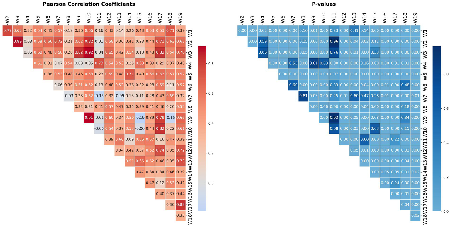
Cross-correlation of groundwater-level time series data between pairwise wells using Pearson test.
The Pearson correlation coefficients between pairwise wells range from −0.19 to 0.92, indicating varying degrees of linear association. Out of 171 well pairs, 163 display positive correlations, while only 8 have negative coefficients. As the absolute value of the correlation increases, a stronger relationship is observed, particularly in positively correlated wells. A total of 95 correlations (56%) are statistically significant (p-value < 0.05). The negative correlations range from −0.19 to −0.01, with none being statistically significant (p-value > 0.05), indicating no meaningful negative correlation among the groundwater-level wells. In contrast, positive correlations range from 0.01 to 0.92. The highest correlation coefficients are found in the subsequent well pairs: W10: W3 (0.92), W10: W9 (0.91), and W2: W3 (0.89). The lowest absolute correlation values are observed in pairs such as W9: W11 (0.01), W2: W11 (−0.01), W4: W9 (0.03), and W7: W8 (−0.03).
It important to mention that all wells with a high number of missing values (W1 W2 W3 W18 W13 W11 W19 W12 W14) exhibit strong to very strong cross-correlation with at least one well that has a low number of missing values (W16 W7 W10 W6 W17W9 W4 W8 W5 W15), except for W18. The highest correlation of this latter is observed with W7 with a Pearson coefficient of 0.57. Pearson and Spearman tests outcome evidence the interest of multivariate analysis use to impute the missing data of a given well, considering as features the time series values of other correlated wells.
3.4.2 SOM clustering
The dataset used for SOM consists of 25-time steps across 19 wells. Eighty rows are discarded, as each contains at least one missing value. Hyperparameter optimization results show that all tested combinations yield test scores ranging between −3.5 and −2.9. These scores indicate that the SOM model operates within a reasonable range and is suitable for assigning wells to clusters for subsequent multivariate analysis aimed at imputing missing groundwater-level (GWL) data.
Despite minimal variation in test scores across different SOM hyperparameter configurations, the resulting clustering structures vary substantially. Notably, the number of singleton clusters ranges from 2 to 19 depending on the parameter settings. This highlights that similar model performance does not necessarily translate into consistent or meaningful cluster groupings.
Since the goal of clustering is to identify groups of wells with similar time series behavior to support cross-well imputation, priority is given to minimizing singleton clusters and maximizing the size of multi-well clusters. The analysis shows that lower epoch values are associated with a higher number of multi-well clusters, suggesting improved grouping cohesion under shorter training durations. Conversely, sigma values greater than 0.5 tend to increase the number of singleton clusters, likely due to the broader neighborhood influence causing cluster dispersion. A lower learning rate generally leads to fewer singleton clusters. Based on these findings, the most favorable hyperparameter combination for balancing clustering relevance and reducing singleton clusters includes a grid size of 5, sigma of 1, learning rate of 0.3, 100 training epochs, and a random seed of 60.
Among the 25 neurons of the 5 × 5 SOM grid, only 9 clusters are occupied, specifically Cluster-0-1, Cluster-1-0, Cluster-1-1, Cluster-1-2, Cluster-1-3, Cluster-2-3, Cluster-3-3, Cluster-4-3, and Cluster-4-4. The most populated cluster is Cluster-1-2, which contains four wells (W2, W3, W10, and W18), followed by Cluster-3-3 with three wells (W6, W12, and W17) (Table 1). Clusters 0–2, 2–1, and 4–4 each contain two wells. Only two wells are isolated in their respective clusters: W8 in Cluster-4-4 and W16 in Cluster-2-3. None of the wells with a high number of missing data belong to singleton clusters. Furthermore, in all clusters where high-missing-data wells are present, they are consistently grouped with at least one well exhibiting low levels of missingness. This co-location enables the use of wells with more complete records as input features for imputing missing values in wells with higher data gaps, enhancing the practical utility of the clustering results for imputation tasks.
Table 1
| SOM cluster | Well | Distance to prototype | Missing data |
|---|---|---|---|
| Cluster-0-1 | W5 | 2.33 | Low |
| W14 | 2.62 | High | |
| W15 | 2.91 | Low | |
| Cluster-1-0 | W6 | 1.95 | Low |
| W12 | 1.87 | High | |
| Cluster-1-1 | W9 | 1.99 | Low |
| W17 | 1.90 | Low | |
| Cluster-1-2 | W2 | 1.20 | High |
| W3 | 1.31 | High | |
| W10 | 1.45 | Low | |
| W18 | 1.23 | High | |
| Cluster-1-3 | W1 | 1.65 | High |
| W7 | 1.74 | Low | |
| Cluster-2-3 | W16 | 2.08 | Low |
| Cluster-4-3 | W4 | 2.84 | Low |
| W11 | 2.39 | High | |
| W13 | 2.82 | High | |
| W19 | 2.18 | High | |
| Cluster-4-4 | W8 | 2.30 | Low |
SOM clustered wells displaying their distance to prototype and missingness data.
The median and standard deviation of the groundwater-level time series dataset are 1.48 and 0.56, respectively. According to criteria established in previous literature (Vesanto and Alhoniemi, 2000; Kohonen, 2013), the quality of fit between a well and its assigned SOM cluster (i.e., the distance to the prototype or neuron weight vector) can be classified into three categories: a good fit corresponds to a distance less than the median (<1.48), a moderate fit is defined as a distance between the median and one standard deviation above the median (1.48–2.04), and a poor fit is indicated by a distance greater than 2.04. Accordingly, a good fit is observed for wells W2, W18, W3, and W10, all of which have distances to their corresponding neuron prototype between 1.20 and 1.45. These wells are assigned to the same cluster (Cluster 1–2), indicating a high degree of internal consistency in their time series patterns. In contrast, W1 and W7, which form Cluster 1–3, exhibit higher distances to the prototype (1.65 and 1.74, respectively), placing them in the moderate fit category. Similarly, moderate fits are observed in Cluster 1–0 and Cluster 1–1, where W12 (1.87), W6 (1.95), W17 (1.90), and W9 (1.99) are located. The remaining wells are relatively distant from their respective cluster centers, indicating weaker associations. Among these, W15 displays the poorest fit, with the highest distance to prototype at 2.91. Supplementary Figure S4 illustrates the temporal patterns of selected wells.
Supplementary Figure S4 reveals that wells that belong to the same cluster exhibit broadly similar time series trajectories, often running in parallel. This parallelism reflects shared socio-environmental drivers such as recharge patterns, extraction pressures, and hydrogeological characteristics. These findings support the approach of imputing missing data in a given well using the complete time series data from other wells within the same cluster.
3.5 Groundwater-level missing values imputation
3.5.1 Uni-well approach
This section evaluates the performance of the models used, ARIMA, RF XGSBoost, and LSTM, for imputing missing groundwater-level data using only the time-series data of the target well. The analysis across 19 monitoring wells employs three error metrics: R2, RRMSE and MAPE and wavelet transformation for variance loss estimation through multi-scale resolution. In addition, a visual inspection is achieved in order to check the reliability of the trajectory.
3.5.1.1 Error metrics model performance analysis
Descriptive statistics of the four models are shown in Figure 6. ARIMA presents the weakest performance, with median scores of R2 = 0.22, RRMSE = 0.33, and MAPE = 15%, with presence of negative R2 values indicators of poor fit. RF shows a moderate but significant improvement over ARIMA, with median values of R2 = 0.54, RRMSE = 0.15, and MAPE = 14%. Both LSTM and XGBoost outperformed the linear and parallel tree-based benchmarks. XGBoost achieves superior median scores of R2 = 0.59, RRMSE = 0.13, and MAPE = 0.11%. LSTM presents the highest R2 median with 0.75 but lower RRMSE (0.14) and MAPE (12%) than XGBoost.
Figure 6
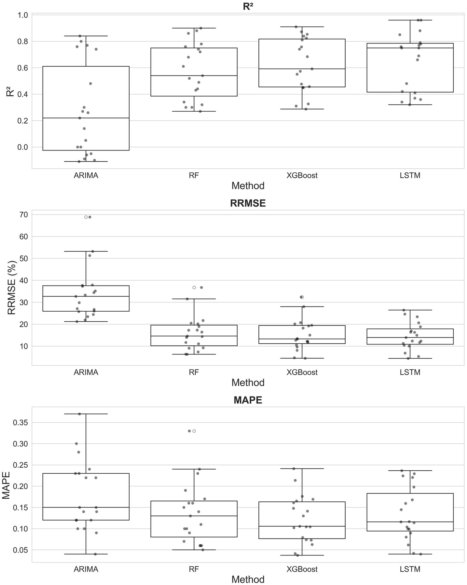
Boxplots of R2, RMSE, and MAPE for univariate groundwater-level predictions of 19 wells using ARIMA, RF, and LSTM.
Figure 7

Original and univariate-predicted time series for wells W7, W8, W12, and W13 using ARIMA, RF, XGBoost, and LSTM.
A well-by-well analysis (Supplementary Figure S5) shows that LSTM achieves the highest R2 in 8 wells, followed by XGBoost in 7, RF in 3, and ARIMA in 1. In terms of error, XGBoost attains the lowest RRMSE in 9 wells and leads in MAPE across 9 wells, followed by LSTM (6 and 4 wells, respectively) and RF (4 and 5 wells), while ARIMA leads in only 1 well for MAPE.
Regarding multi-metric dominance, XGBoost achieves a “clean sweep” across all three metrics in 5 wells and near-dominance in 1; LSTM achieves a clean sweep in 4 wells and dominance in 1. RF does not achieve any clean sweep and dominates only one well, and ARIMA achieves neither.
3.5.1.2 Wavelet-based multi-scale performance analysis
The Total Variance Loss metric provides a multi-scale assessment of each model’s ability to preserve signal structure.
XGBoost achieves the best variance preservation in 11 of 19 wells. Eight wells exhibit near-zero variance loss (0.01–1.1%), and five remain below 15%. However, the model fails in three wells, including two extreme cases (66 and 81% loss). This pattern persists across decomposition levels, with a single small negative loss (−0.82%) appearing at Level 3.
LSTM performs best in 7 wells and maintains moderate, stable variance loss (4–30%) for most wells, with three wells reaching 53% loss. One near-zero negative value (−0.3%) appears. This behavior remains consistent across all levels.
RF leads in 3 wells and exhibits variance loss between 9 and 58%. Across all levels it shows high, relatively stable variance loss (typically 30–67%), indicating oversmoothing.
ARIMA performs best in 4 wells but generates extreme negative variance-loss values across levels (as low as −209% at Level 3), indicating artificial signal creation, and extreme positive values up to 81%, indicating failure to capture underlying components.
3.5.1.3 Visual analysis of the performance across missing data patterns
The visual analysis is carried out by jointly plotting the historical (original) time series and the model-predicted series for each well. In this section, the interpretation is structured according to the missing-data patterns identified through HCA (Section 2.2). Each pattern is illustrated using a representative well.
Pattern 1: Isolated missing values – Representative well: W7
This pattern includes five wells. The smooth temporal dynamics and low density of missing values allow all four models to achieve high accuracy. In general, the predicted trajectories closely follow the original series, with absolute deviations generally limited to a few centimeters. The main discrepancies arise when the original time series exhibits abrupt, spike-like deviations from its local neighborhood. In these instances, XGBoost most accurately reproduces the sharp variations, while RF and MICE generate slightly smoother responses, and LSTM tends to produce more abrupt reactions.
Pattern 2: Isolated values with a terminal Gap – Representative well: W8.
This pattern also contains five wells and behaves similarly to Pattern 1, though model differences become more pronounced during abrupt fluctuations.
Differences become more pronounced around sharp spikes: RF and ARIMA tend to smooth these variations, and XGBoost and LSTM follow the original trajectory more accurately, with XGBoost clearly outperforming the others. In the terminal gap, the two tree-based models produce similar estimates, LSTM diverges, and MICE fails to provide any imputation. At the start of the series, LSTM does not generate predictions because its internal state is initialized without meaningful context, resulting in no early outputs until sufficient sequential information is accumulated.
Pattern 3: Initial gap with isolated values – Representative wells W3
The pattern includes five wells. Pattern five is presented here because both exhibit similar behaviors.
During the initial gap, ARIMA, RF, and XGBoost generally produce an almost constant imputed value across the missing segment, with RF and XGBoost generating similar outputs. In contrast, LSTM captures the overall trend but introduces suspicious spikes that exceed the original data range, due to insufficient information for state initialization. Outside the gap, XGBoost and LSTM more accurately reproduce the dynamics of the original series, followed by RF, while ARIMA performs considerably worse.
Pattern 4: Initial and terminal gaps – Representative well: W13
Four wells fall into this category. Visual inspection highlights a major limitation: in the absence of any initial target values, RF, XGBoost, and LSTM default to imputing nearly constant values, while ARIMA fails to produce meaningful predictions. This illustrates a fundamental constraint of univariate imputation when no historical data are available to initialize the model. At the end of the series, where another gap occurs, model responses vary markedly—differences may exceed five meters. LSTM shows the largest deviations, often producing pronounced spikes. When observed data are available, XGBoost consistently provides the closest match to the original series.
Visual assessment across all patterns highlights method-specific behaviors: RF exhibits systematic oversmoothing, ARIMA produces unstable and often erratic estimates, XGBoost consistently reproduces the original series with high fidelity, and LSTM performs well in low-variability segments but loses reliability in the presence of frequent or pronounced spikes. As the magnitude and frequency of local fluctuations increase, discrepancies among the four methods become more pronounced, reflecting their differential sensitivity to sharp temporal variations and their limitations in handling large gaps or extensive missing-data patterns.
3.5.2 Multi-well approach
To address wells with high rates of missing data, a multivariate approach was implemented. This method imputes missing values in a target well by leveraging time series from other wells with similar hydrological behavior, using them as auxiliary features. RF, XGBoost and LSTM models were applied in this phase. ARIMA was excluded due to its previously demonstrated lower performance and inherent inability to incorporate external variables and replaced by MICE with BaysianRidge model which is a multivariate method for imputing missing data.
3.5.2.1 Auxiliary well selection
Multivariate imputation is performed only for wells with a high proportion of missing values (W1, W2, W3, W11, W12, W13, W14, W18, and W19). The workflow begins with Pearson and Spearman cross-correlation analyses, along with SOM clustering applied to the full set of wells in order to identify, for each target well, the wells with which it is most strongly related. The selected wells are then incorporated as auxiliary features in the MICE, Random Forest, XGBoost, and LSTM models to impute the missing values in the target well’s time series.
Auxiliary features are chosen using two criteria:
-
The well whose time series exhibits the highest Pearson/Spearman cross-correlation with the target well.
-
The wells that fall within the same SOM cluster as the target well.
Based on these criteria, three feature combinations are constructed (Table 2). The first includes only the single most highly correlated well. The second includes all wells assigned to the same SOM cluster as the target well. The third combines both sources: the most correlated well together with the SOM-clustered wells. In every case, the available observations from the target well itself are included as part of the input to the imputation models.
Table 2
| Target well | Multivariate features | ||
|---|---|---|---|
| Best cross-correlated (Pearson/Spearman) | Cluster (SOM) | Pearson/Spearman + SOM | |
| W1 | W10 | W7 | W7, W10 |
| W2 | W10 | W3, W10, W18 | |
| W3 | W10 | W2, W10, W18 | |
| W11 | W4 | W4, W13, W19 | |
| W12 | W17 | W6 | W6, W17 |
| W13 | W15 | W4, W11, W19 | W4, W11, W15, W19 |
| W14 | W5 | W5, W15 | |
| W18 | W7 | W2, W3, W10 | W2, W3, W7, W10 |
| W19 | W17 | W4, W11, W13 | W4, W11, W13, W17 |
Combinations of features used for multi-well analysis.
According to Table 2 the multi-well prediction of groundwater-level for wells W2, W3, W11, and W14 is performed comparing two-feature0 combinations, while for wells W1, W12, W13, W18, and W19 is modeled comparing three-feature combinations. In the former group, the most strongly Pearson cross-correlated well belongs to the same SOM cluster as the target well, whereas in the latter group, it lies outside the target well’s SOM cluster.
3.5.2.2 Overall model performance in the multivariate setting
Descriptive statistics for R2, RRMSE, and MAPE, along with their distributions (Figure 8), indicate that among the tested methods, MICE performs the weakest (median R2 = 0.39, RRMSE = 0.16, MAPE = 12%), followed by Random Forest (R2 = 0.45, RRMSE = 0.11, MAPE = 10%). XGBoost and LSTM provide the strongest benchmarks, with median R2 of 0.50 and 0.52, RRMSE of 0.12 and 0.14, and MAPE of 10 and 11%, respectively.
Figure 8

Boxplots of R2, RMSE, and MAPE for multivariate groundwater-level predictions of 9 wells using MICE, RF, XGBoost, and LSTM.
A well-by-well evaluation using the three error metrics shows XGBoost as the top-performing model, ranking first in 6 of 9 wells based on R2 (including W2: 0.91, W3: 0.88, W18: 0.93), in 5 wells for RRMSE, and 4 wells for MAPE. LSTM ranks second, matching or outperforming other methods in 2 wells for R2, 3 wells for RRMSE, and 2 wells for MAPE. MICE_Bayesian follows (2, 1, 1 wells), while RF ranks last (0, 1, 1 wells). MICE exhibits extreme negative R2 values in some wells (e.g., W18: –3.79, W14: −1.15), indicating complete failure. Detailed well-level metrics are provided in Supplementary Figure S6.
A “clean sweep” analysis shows XGBoost dominates all three metrics in 5 wells, LSTM and MICE achieve a clean sweep in 1 well each, and RF dominates only 1 well.
3.5.2.3 Comparative effectiveness of auxiliary wells selection methods
SOM-based or combined feature sets achieve higher R2 than Pearson correlation by using multiple auxiliary wells to reduce noise and enhance trends, despite relying on fewer data due to the need for a complete, gap-free dataset, whereas Pearson typically selects a single feature, is more noise-sensitive, but can exploit all pairwise time series.
Using SOM-based feature selection, R2 improves from univariate to multivariate models as the distance between an auxiliary well and its SOM prototype decreases, reflecting higher informational relevance. XGBoost shows the largest R2 gain, with performance deteriorating beyond a prototype distance of ~2.18, indicating detrimental noise. Sensitivity thresholds are lower for LSTM (1.65) and RF (1.31), with maximum R2 improvements of 0.29 (XGBoost), 0.18 (RF), and 0.04 (LSTM).
Across other metrics and variance-loss levels, no consistent relationship or method preference is observed, suggesting that performance is primarily governed by the intrinsic structure of the auxiliary data and localized hydrological or anthropogenic influences.
3.5.2.4 Wavelet-based multi-scale performance analysis
A multi-resolution wavelet analysis assesses each method’s ability to preserve variance across temporal scales:
XGBoost: Total variance loss ranges from −0.6 to 78.9% (median 23.7%). Excellent preservation (<10% loss) occurs in 4 cases, good-to-acceptable (10–30%) in 11, and high-loss (>30%) in 8 wells. Low-frequency Level 0 shows improved performance with 4 excellent and 13 good-to-acceptable cases, though Levels 1–2 deteriorate, with 15 high-loss cases, and Level 3 recovers with over half the cases in excellent-to-acceptable range.
LSTM: Loss ranges from −6.3 to 32.9% (median 7.7%), showing balanced performance with 9 excellent (<10%) and 6 good (10–20%) cases; only 1 case exceeds 30% loss. Negative losses occur in 4 wells, increasing to 7 at Level 0. Levels 1–3 show gradual performance decrease, with up to 9 high-loss cases and negative losses from 5 to 9%.
RF: Loss ranges from 16.7 to 71.4% (median 52.8%), exhibiting poor preservation. No excellent cases exist, and 17 exceed 30% loss. Level 0 shows minimal improvement (2 excellent cases, 12 high-loss), deteriorating at higher levels where all cases exceed 30% loss. No negative values are observed.
MICE: Loss ranges from 4.4 to 28.8% (median 18.2%), with 4 excellent and 19 good-to-acceptable cases. High-loss failures are absent. Level 0 maintains stability (5 excellent, 14 good), Level 1 shows increased variability with 5 negative cases, Level 2 shows 12 negative cases, and Level 3 recovers with 6 negative cases and only 3 high-loss failures.
3.5.2.5 Performance across missing data patterns
The visual analysis is performed by plotting the historical time series alongside model-predicted series for each well across the three auxiliary feature sets. Two representative wells, W12 and W13, illustrate the observed behaviors (Figures 9, 10).
Figure 9
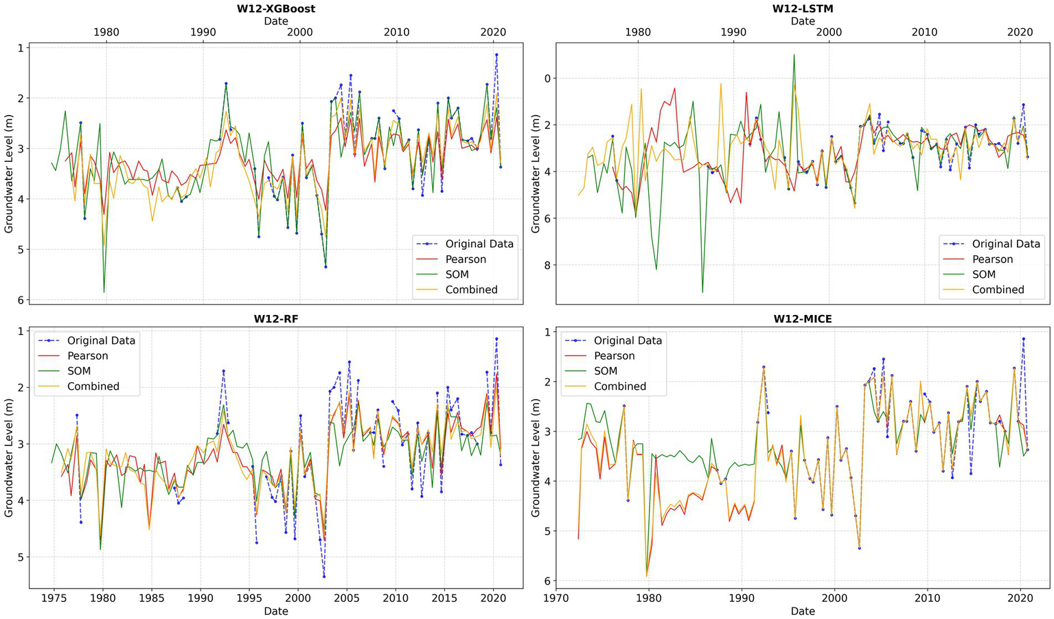
Original and multivariate-predicted time series for W12 using MICE, RF, XGBoost, and LSTM with different auxiliary feature sets.
Figure 10

Original and multivariate-predicted time series for W13 using MICE, RF, XGBoost, and LSTM with different auxiliary feature sets.
Visual inspection reveals that gaps in univariate predictions, often filled with constant values, are replaced by more realistic estimates when auxiliary feature sets are incorporated, capturing the seasonal dynamics of groundwater-level variations. Leveraging sufficient information from auxiliary wells, LSTM overcomes its typical limitation in predicting initial sequence values, enabling forecasts across the entire early period.
The analysis also highlights sensitivity to auxiliary feature selection, which standard metrics do not capture. RF exhibits the lowest sensitivity, followed by XGBoost, while MICE shows greater variability. LSTM is the most sensitive, with minor perturbations in input features occasionally producing divergent forecasts and physically unrealistic trajectories that, in some cases, exceed genuine groundwater-level ranges, reflecting amplification of noise rather than underlying data patterns.
4 Discussion
4.1 Uni-well
The evaluation of LSTM, RF, XGBoost, and ARIMA models for univariate imputation of missing groundwater-level (GWL) data in the Grombalia shallow aquifer reveals a fundamental trade-off between statistical fidelity, point prediction accuracy and visual inspection.
XGBoost shows the strongest overall performance, achieving an effective balance between accurate point predictions and preservation of statistical characteristics. It maintains near-perfect variance across frequency components and reliably captures multi-scale temporal dependencies. This low variance loss is consistent across wells, suggesting an inherent strength of the method rather than a site-dependent artifact. Visual inspection confirms its ability to reproduce abrupt, step-like seasonal shifts without distortion, maintaining realistic trajectories. These advantages stem from XGBoost’s sequential boosting and regularization, which reduce error propagation and ensure stability even in the presence of missing data. This combination of reliability and fidelity positions XGBoost as the most robust univariate imputation approach.
LSTM exhibits a different performance profile, offering high point prediction accuracy but moderate statistical fidelity. It captures temporal dependencies across scales, although less effectively than XGBoost. Visual inspection shows that LSTM predictions generally follow the original data, but trajectories can deviate and sometimes exceed the natural dynamic range of GWL fluctuations. Additionally, the model often leaves the initial portion of the series unimputed because it requires a minimum sequence length to initiate forecasting, a limitation not shared by XGBoost, which uses lagged features directly.
RF performs considerably worse, combining moderate prediction accuracy with substantial variance loss across all frequency components. This reflects systematic over-smoothing in the majority of wells. Visual inspection confirms that RF fails to capture abrupt seasonal spikes, producing flattened trajectories that underrepresent the full dynamic range of GWL fluctuations. These limitations arise from the model’s lack of temporal memory, which restricts its ability to capture long-term dependencies. Although flexible and distribution-agnostic, RF consistently smooths high-frequency variability, limiting its ability to preserve chronological structure.
ARIMA displays the weakest and least consistent performance. Its assumptions of linearity and stationarity are frequently violated in groundwater systems influenced by seasonal recharge, pumping, and land-use changes. As a result, ARIMA often produces low prediction accuracy, unstable variance preservation, and occasionally even negative R2 values. Visual inspection highlights its tendency to generate linear, interval-like trends that fail to capture the variability characteristic of GWL time series. These outcomes indicate that ARIMA is fundamentally unsuited for imputing missing groundwater data in nonlinear, seasonally driven systems.
Across the complete performance spectrum, XGBoost remains the strongest univariate model for GWL imputation. However, it still struggles to capture nonlinear dynamics in a subset of wells, likely due to noisy site-specific data or intrinsic limitations in representing certain data signals. In a few isolated cases, even the generally weakest models may outperform it.
A common limitation across all methods is their behavior during extended data gaps. When gaps occur at the beginning of the series, XGBoost, LSTM, and RF often default to imputing near-constant values, while ARIMA may fail outright. When gaps appear in the middle of the record, almost none of the models successfully reconstruct the underlying trend. This shared univariate limitation underscores the need for multivariate imputation strategies that incorporate auxiliary information, such as data from cross-correlated wells, to meaningfully improve reconstruction accuracy.
4.2 Muli-well
XGBoost exhibits consistently high point-prediction accuracy and strong statistical fidelity, particularly at low-frequency levels, demonstrating a robust ability to capture large-scale groundwater trends. While a subset of wells displays elevated loss values indicative of oversmoothing, XGBoost remains the best-performing model at higher-frequency levels, where variance preservation is most critical for imputation. Even though some wells still experience substantial variance loss, the method most reliably retains the intrinsic high-frequency signal structure.
The LSTM model achieves point-prediction accuracy comparable to XGBoost and shows similar overall variance preservation. However, it exhibits a higher incidence of negative values, suggesting that its recurrent architecture may artificially inflate variance and introduce spurious high-frequency fluctuations in certain wells. These distortions highlight the model’s sensitivity to both data quality and feature configuration.
Random Forest demonstrates moderate to low point-prediction accuracy and consistently poor variance preservation across most wells. The model systematically oversmooths the data—particularly at high-frequency levels, where variance loss exceeds 40% for all cases. While RF can approximate long-term trends and produce reasonable point estimates, its lack of temporal memory introduces a structural bias that suppresses inherent high-frequency variability. This limitation reflects a fundamental inability to capture short-term dynamics and the hierarchical temporal structure characteristic of groundwater systems.
MICE shows the lowest point-prediction accuracy but performs exceptionally well at preserving variance at the coarsest frequency decomposition (Level 0). At deeper decompositions, however, it deteriorates sharply, exhibiting frequent negative-value occurrences and numerous high-loss cases. This behavior is inherent to MICE: although it reliably preserves low-frequency, broad-scale relationships between variables, it cannot reconstruct fine-scale stochastic components of the time series. The uncertainty introduced through Bayesian Ridge Regression parameters and residual noise does not translate into realistic variance preservation at higher frequencies.
Visual inspection of trajectory curves further reveals discrepancies not captured by standard metrics. XGBoost, Random Forest, and MICE generally produce smooth, physically plausible trajectories during gap-filling, whereas LSTM frequently generates distorted shapes and unrealistic amplitudes. These failure modes stem from known limitations of deep recurrent models under data scarcity: cold-start instability, where uninformative initial states corrupt early predictions, and feature-sensitivity instability, where small perturbations in auxiliary wells produce disproportionately large deviations in reconstructed trajectories. Together, these issues reflect the inherently high variance of recurrent architectures when trained on sparse hydrological datasets.
In contrast, XGBoost’s robustness arises from its inductive biases: the absence of temporal state prevents error accumulation, and its strong regularization mechanisms promote low-variance, stable predictions across different feature subsets. These characteristics make XGBoost particularly well suited for groundwater-level imputation in data-limited environments such as the Grombalia shallow aquifer.
Overall, the performance hierarchy places XGBoost as the leading model, with LSTM showing competitive aggregate metrics but yielding unrealistic trajectories in several cases, and Random Forest and MICE emerging as weaker alternatives. However, this hierarchy is not absolute. XGBoost occasionally oversmooths individual wells, and the other models produce competent results under specific conditions. This variability underscores the need for well-specific validation.
Finally, predictive accuracy depends critically on feature selection. While incorporating multiple auxiliary wells can reduce noise and better capture trends than single-well correlation-based selection, this is not universally true. The usefulness of an auxiliary well decreases with its dissimilarity to the target series, highlighting the need for careful, well-specific feature choice. Optimal imputation therefore requires jointly considering model architecture and feature selection rather than relying on a single, universal approach.
4.3 Optimal prediction method for each well: univariate versus multivariate analysis
To determine the optimal prediction method for each well under univariate and multivariate scenarios, a feasibility framework was developed. The framework combines standard error metrics with wavelet-based multi-resolution analysis and classifies performance into five categories based on thresholds for accuracy and temporal-structure preservation (Table 3). It is applied to 19 wells using four univariate methods and to 9 wells using three multivariate feature sets. Visual inspection is used to break ties between methods and to verify whether statistically acceptable models generate realistic trajectories, especially across gap periods. This analysis quantifies the proportion of wells for which prediction is feasible and clarifies how performance changes when moving from univariate to multivariate modeling.
Table 3
| Category | R2 | RRMSE (%) | MAPE | Total variance loss (%) |
|---|---|---|---|---|
| Excellent | > 0.85 | < 11 | < 0.11 | < 10 |
| Very good | 0.85–0.74 | 11–16 | 0.11–0.16 | 10–15 |
| Good | 0.74–0.65 | 16–19 | 0.16–0.19 | 15–25 |
| Acceptable | 0.65–0.60 | 19–25 | 0.19–0.25 | 25–35 |
| Unacceptable | < 0.60 | > 25 | > 0.25 | > 35 |
Feasibility framework for groundwater-level missing data imputation.
Statistical results show that 58% of wells (9/19) achieve Very Good to Acceptable performance in the univariate case, increasing to 67% (5/9) in the multivariate case. After visual inspection, the number of reliable univariate predictions decreases considerably, as most univariate models fail to reconstruct plausible trajectories over long gaps. This underscores the advantage of multivariate modeling for both prediction and imputation. Exceptions exist, for example well W3, where univariate and multivariate trajectories are similarly realistic despite lower univariate metrics. Figure 11 illustrates typical improvements (W13, W18, W1) and an example of similar performance (W3).
Figure 11

Examples of multivariate improvements compared to univariate predictions and a case of similar performance.
Overall, multivariate models generally improve or maintain predictive skill and offer a key operational advantage which is the ability to impute extensive gaps, including early missing segments, with XGBoost performing particularly well. Implementing a multi-well analysis framework, however, does entail higher computational demands than single-well approaches, which may pose challenges in low-resource operational settings. Yet, recent advances in high-performance, cost-efficient computing have greatly mitigated these constraints, enabling agencies to more readily incorporate auxiliary well information to enhance imputation accuracy. This is further facilitated by the fact that GWL monitoring networks are typically managed by a single authority, with all well and piezometer time series stored in a unified database that supports integrated processing and model coupling. As a result, the main practical limitation is less a matter of computational capacity and more the identification and optimization of appropriate auxiliary wells, along with the correct implementation of the analytical methodology for each target well. Notably, the optimal feature-set complexity is well-dependent, reflecting both localized and network-scale hydrogeological interactions. Instances of poor performance highlight the need to incorporate additional physical drivers, such as precipitation, evapotranspiration, and groundwater extraction, and/or to employ alternative or hybrid modeling approaches better suited to the specific groundwater-level dynamics of individual wells.
5 Conclusion
GWL imputation and forecasting are conducted under challenging hydrogeological and data-limited conditions using both uni-well and multi-well time-series analyses. Five models representing distinct methodological families are applied: classical statistical approaches (ARIMA, MICE), ensemble-based machine learning (RF, XGBoost), and sequential deep learning (LSTM). Model performance is assessed within a feasibility framework that integrates standard error metrics (R2, RMSE, MAPE), wavelet-based multi-resolution analysis, and visual inspection, allowing consistent classification from Excellent to Unacceptable imputation and ensuring the physical realism of reconstructed trajectories, particularly across long gaps.
The study focuses on the Grombalia shallow aquifer, a hydrologically complex Mediterranean semi-arid system influenced by multiple interacting drivers, including diverse irrigation sources, artificial and natural recharge, drainage infrastructure, ephemeral and perennial wadis, licit and illicit groundwater abstraction, and pronounced intra- and interannual rainfall variability. The GWL dataset, measured only twice a year, is sparse, irregular, and sensitive to climate anomalies, posing significant challenges for imputation.
In the univariate setting, only 58% of wells achieve Very Good to Acceptable performance, and visual inspection further reduces the number of credible predictions due to unrealistic behavior across long gaps. XGBoost consistently delivers the strongest performance, preserving both low- and high-frequency dynamics and maintaining stable behavior across wells with varying data characteristics and degrees of missingness. LSTM performs competitively but cannot predict at the beginning of the series due to lag-window requirements. RF performs moderately but oversmooths high-frequency fluctuations, while ARIMA struggles to capture nonlinear and irregular groundwater dynamics. All uni-well approaches exhibit limitations in imputing extended early-series gaps.
Multivariate modeling substantially improves imputation, particularly for early-period gaps that uni-well methods fail to reconstruct. Overall metrics improve, increasing the proportion of wells with feasible predictions to 67%. XGBoost maintains robust performance and clearly outperforms other methods. LSTM often produces exaggerated trajectories under sparse or fragmented auxiliary data, RF continues to oversmooth, and MICE captures broad trends but fails to reproduce fine-scale variability. Feature selection using SOM-based clustering generally outperforms correlation-based methods, though no single approach is optimal for all wells. In some cases, combining clustering and correlation provides the most reliable solution.
Despite these improvements, extended gaps and sparse monitoring continue to challenge all approaches, and more than 30% of wells remain infeasible when relying solely on GWL data. Nonetheless, relying only on groundwater monitoring networks offers practical advantages, including no exogenous data needed, automated processing, reduced computational demands, and simplified operational implementation. Enhancing performance further requires incorporating additional physical drivers, such as precipitation, evapotranspiration, and remote-sensing indicators, and exploring hybrid or well-specific modeling strategies. Advanced temporal architectures, including Temporal Convolutional Networks and attention-based models (e.g., Transformers), may also be explored, as they can capture long-range dependencies and reduce error propagation, although they remain computationally intensive and uncertain under sparse, biannual, or irregular time-series data.
Statements
Data availability statement
The original contributions presented in the study are included in the article/Supplementary material, further inquiries can be directed to the corresponding author.
Author contributions
HS: Formal analysis, Visualization, Data curation, Writing – original draft, Validation, Investigation, Software. AO: Conceptualization, Validation, Writing – review & editing, Funding acquisition. SP: Validation, Conceptualization, Writing – review & editing. MA: Funding acquisition, Writing – original draft, Supervision, Writing – review & editing, Software, Methodology, Conceptualization, Validation.
Funding
The author(s) declared that financial support was received for this work and/or its publication. This research was supported by the Ministry of High Education and Scientific Research of Tunisia (MESRS) in the framework of the Contrat-Programme and by the University of Montpellier.
Conflict of interest
The author(s) declared that this work was conducted in the absence of any commercial or financial relationships that could be construed as a potential conflict of interest.
Generative AI statement
The author(s) declared that Generative AI was not used in the creation of this manuscript.
Any alternative text (alt text) provided alongside figures in this article has been generated by Frontiers with the support of artificial intelligence and reasonable efforts have been made to ensure accuracy, including review by the authors wherever possible. If you identify any issues, please contact us.
Publisher’s note
All claims expressed in this article are solely those of the authors and do not necessarily represent those of their affiliated organizations, or those of the publisher, the editors and the reviewers. Any product that may be evaluated in this article, or claim that may be made by its manufacturer, is not guaranteed or endorsed by the publisher.
Supplementary material
The Supplementary material for this article can be found online at: https://www.frontiersin.org/articles/10.3389/frwa.2025.1726853/full#supplementary-material
References
1
Agwu O. E. Akpabio J. U. Dosunmu A. (2020). Artificial neural network model for predicting the density of oil-based muds in high-temperature, high-pressure wells. J. Pet. Explor. Prod. Technol.10, 1081–1095. doi: 10.1007/s13202-019-00802-6
2
Alley W. M. Reilly T. E. Franke O. L. (1999). Sustainability of ground-water resources. Denver, CO: U.S. Dept. of the Interior.
3
Asgharinia S. Petroselli A. (2020). A comparison of statistical methods for evaluating missing data of monitoring wells in the Kazeroun plain, Fars Province, Iran. Groundw. Sustain. Dev.10:100294. doi: 10.1016/j.gsd.2019.100294
4
Astuti W. Govindaraju R. (2026). Effect of data gaps on harmful algal bloom prediction models for inland lakes. J. Hydrol. Eng.31:04025045. doi: 10.1061/JHYEFF.HEENG-6544
5
Baste S. Klotz D. Acuña Espinoza E. Bardossy A. Loritz R. (2025). Unveiling the limits of deep learning models in hydrological extrapolation tasks. Hydrol. Earth Syst. Sci.29, 5871–5891. doi: 10.5194/hess-29-5871-2025
6
Belkhiri L. Boudoukha A. Mouni L. Baouz T. (2010). Application of multivariate statistical methods and inverse geochemical modeling for characterization of groundwater — a case study: Ain Azel plain (Algeria). Geoderma159, 390–398. doi: 10.1016/j.geoderma.2010.08.016
7
Ben-Salem N. Anane M. Jomaa S. Jellali S. (2019). Hydrolink 2019/3. Impact of anthropogenic activities on physiochemical properties of wadi el bey (northeast of Tunisia). Madrid: International Association for Hydro-Environment Engineering and Research (IAHR). S. 70–73.
8
BICHE . (2020). Projet d’intensification de l’agriculture irriguée en Tunisie (P.I.A.I.T). Plan de Gestion Environnementale et Sociale (PGES) du projet d’assainissement et de drainage dans les ppi de grombalia – béni khalled - menzel bouzelfa et soliman. Rapport définitif modifié. Available online at: http://www.agriculture.tn/wp-content/uploads/2020/07/PGES-drainage-Nabeul-DEF-modifie%CC%81-Juin-2020-_RevMC-2.pdf (accessed December 30 2025).
9
Bikše J. Retike I. Haaf E. Kalvāns A. (2023). Assessing automated gap imputation of regional scale groundwater level data sets with typical gap patterns. J. Hydrol.620:129424. doi: 10.1016/j.jhydrol.2023.129424
10
Boualoulou N. Belhoussine Drissi T. Nsiri B. (2022). An intelligent approach based on the combination of the discrete wavelet transform, delta delta MFCC for Parkinson’s disease diagnosis. Int. J. Adv. Comput. Sci. Appl.13:466. doi: 10.14569/IJACSA.2022.0130466
11
Bouteraa O. Mebarki A. Bouaicha F. Nouaceur Z. Laignel B. (2019). Groundwater quality assessment using multivariate analysis, geostatistical modeling, and water quality index (WQI): a case of study in the boumerzoug-el khroub valley of Northeast Algeria. Acta Geochim.38, 796–814. doi: 10.1007/s11631-019-00329-x
12
Box G. E. P. Jenkins G. M. (1976). Time series analysis: Forecasting and control. Revised Edn. San Francisco, California: Holden Day.
13
Box G. E. Jenkins G. M. Reinsel G. C. Ljung G. M. (2015). Time series analysis: Forecasting and control. 5th Edn. New Jersey: Wiley.
14
Breiman L. (2001). Random Forest. Mach. Learn.45, 5–32. doi: 10.1023/A:1010933404324
15
Chai T. Draxler R. R. (2014). Root mean square error (RMSE) or mean absolute error (MAE)? -arguments against avoiding RMSE in the literature. Geosci. Model Dev.7, 1247–1250. doi: 10.5194/gmd-7-1247-2014
16
Chan W.-S. (1999). A comparison of some of pattern identification methods for order determination of mixed ARMA models. Stat. Probab. Lett.42, 69–79. doi: 10.1016/S0167-7152(98)00195-3
17
Chang Y.-W. Sun W. Kow P.-Y. Lee M.-H. Chang L.-C. Chang F.-J. (2025). Advanced groundwater level forecasting with hybrid deep learning model: tackling water challenges in Taiwan’s largest alluvial fan. J. Hydrol.655:132887. doi: 10.1016/j.jhydrol.2025.132887
18
Chen T. Guestrin C. (2016) XGBoost: a scalable tree boosting system., in Proceedings of the 22nd ACM SIGKDD international conference on knowledge discovery and data mining, (San Francisco California: ACM), 785–794.
19
Clark S. Hyndman R. J. Pagendam D. Ryan L. M. (2020). Modern strategies for time series regression. Int. Stat. Rev.88, S179–S204. doi: 10.1111/insr.12432
20
Dandapat A. K. Panda P. K. Sankalp S. Kisi O. Kraiem H. Kucher O. D. et al . (2025). Ensemble deep learning framework for groundwater storage forecasting under hydrological variability. Acta Geophys.74:1. doi: 10.1007/s11600-025-01735-x
21
Daughney C. J. Raiber M. Moreau-Fournier M. Morgenstern U. Van Der Raaij R. (2012). Use of hierarchical cluster analysis to assess the representativeness of a baseline groundwater quality monitoring network: comparison of New Zealand’s national and regional groundwater monitoring programs. Hydrogeol. J.20, 185–200. doi: 10.1007/s10040-011-0786-2
22
Deng Y. Chang C. Ido M. S. Long Q. (2016). Multiple imputation for general missing data patterns in the presence of high-dimensional data. Sci. Rep.6:21689. doi: 10.1038/srep21689,
23
Deng J. Couasnon A. Dahm R. Hrachowitz M. Van Heeringen K.-J. Korving H. et al . (2024). Operational low-flow forecasting using LSTMs. Front. Water5:1332678. doi: 10.3389/frwa.2023.1332678
24
DGRE (2005) Annuaire piézométrique de la Tunisie 2005. Tunis. Tunisia: DGRE.
25
DGRE (2019) Annuaire de l’exploitation des nappes souterraines de l’année 1979–2019. Tunis. Tunisia: DGRE.
26
Díaz-Uriarte R. Alvarez de Andrés S. (2006). Gene selection and classification of microarray data using random forest. BMC Bioinform.7:3. doi: 10.1186/1471-2105-7-3,
27
Dwivedi D. Mital U. Faybishenko B. Dafflon B. Varadharajan C. Agarwal D. et al . (2022). Imputation of contiguous gaps and extremes of subhourly groundwater time series using random forests. J. Mach. Learn. Model. Comput.3, 1–22. doi: 10.1615/JMachLearnModelComput.2021038774
28
El Garouani M. Radoine H. Lahrach A. Jarar Oulidi H. (2022). Spatiotemporal analysis of groundwater resources in the Saïss aquifer, Morocco. Water15:105. doi: 10.3390/w15010105
29
Engels J. (2003). Imputation of missing longitudinal data: a comparison of methods. J. Clin. Epidemiol.56, 968–976. doi: 10.1016/S0895-4356(03)00170-7,
30
Evans S. W. (2020). Groundwater level mapping tool: an open source web application for assessing groundwater sustainability. Environ. Model. Softw.131:104782. doi: 10.1016/j.envsoft.2020.104782
31
Feng F. Ghorbani H. Radwan A. E. (2024). Predicting groundwater level using traditional and deep machine learning algorithms. Front. Environ. Sci.12:1291327. doi: 10.3389/fenvs.2024.1291327
32
Fleet P. J. V. (2019). Discrete wavelet transformations: An elementary approach with applications. 2nd Edn. University of St. Thomas: Wiley.
33
Gaaloul N. Candela L. Chebil A. Soussi A. Tamoh K. (2014). Groundwater flow simulation at the Grombalia phreatic aquifer (cap bon, northeastern Tunisia). Desalin. Water Treat.52, 1997–2008. doi: 10.1080/19443994.2013.821026
34
Gleeson T. Wada Y. Bierkens M. F. P. van Beek L. P. H. (2012). Water balance of global aquifers revealed by groundwater footprint. Nature488, 197–200. doi: 10.1038/nature11295,
35
Güler C. Thyne G. D. McCray J. E. Turner K. A. (2002). Evaluation of graphical and multivariate statistical methods for classification of water chemistry data. Hydrogeol. J.10, 455–474. doi: 10.1007/s10040-002-0196-6
36
Hochreiter S. Schmidhuber J. (1997). Long short-term memory. Neural Comput.9, 1735–1780. doi: 10.1162/neco.1997.9.8.1735,
37
Hosseini S. H. Moeini R. (2025). Correlation–based reliability index equipped with machine learning methods to complete the groundwater level gaps. Results Eng.25:104146. doi: 10.1016/j.rineng.2025.104146
38
Hyndman R. J. Koehler A. B. (2006). Another look at measures of forecast accuracy. Int. J. Forecast.22, 679–688. doi: 10.1016/j.ijforecast.2006.03.001
39
Jaxa-Rozen M. Kwakkel J. (2018). Tree-based ensemble methods for sensitivity analysis of environmental models: a performance comparison with Sobol and Morris techniques. Environ. Model. Softw.107, 245–266. doi: 10.1016/j.envsoft.2018.06.011
40
Jeong J. Park E. Han W. S. Kim K. Choung S. Chung I. M. (2017). Identifying outliers of non-Gaussian groundwater state data based on ensemble estimation for long-term trends. J. Hydrol.548, 135–144. doi: 10.1016/j.jhydrol.2017.02.058
41
Junninen H. Niska H. Tuppurainen K. Ruuskanen J. Kolehmainen M. (2004). Methods for imputation of missing values in air quality data sets. Atmos. Environ.38, 2895–2907. doi: 10.1016/j.atmosenv.2004.02.026
42
Kenda K. Čerin M. Bogataj M. Senožetnik M. Klemen K. Pergar P. et al . (2018). “Groundwater modeling with machine learning techniques: Ljubljana Polje aquifer” in Proceedings, vol. 2, 697. doi: 10.3390/proceedings2110697
43
Kim J.-Y. Oh J.-S. (2023). Multiple feature extraction Long short-term memory using skip connections for ship electricity forecasting. J Mar Sci Eng11:1690. doi: 10.3390/jmse11091690
44
Kingma D. P. Ba J. (2017). Adam: a method for stochastic optimization. arXiv [Preprint] doi: 10.48550/arXiv.1412.6980
45
Kio A. E. Xu J. Gautam N. Ding Y. (2024). Wavelet decomposition and neural networks: a potent combination for short term wind speed and power forecasting. Front. Energy Res.12:1277464. doi: 10.3389/fenrg.2024.1277464
46
Kohonen T. (1982). Self-organized formation of topologically correct feature maps. Biol. Cybern.43, 59–69. doi: 10.1007/BF00337288
47
Kohonen T. (2013). Essentials of the self-organizing map. Neural Netw.37, 52–65. doi: 10.1016/j.neunet.2012.09.018,
48
Kumari S. Singh S. K. (2025). “An artificial bee colony optimized LSTM model to multivariate prediction of sdg 8 indicators” in AI technologies for information systems and management science. eds. GargL.KesswaniN.BriguiI. (Cham: Springer Nature Switzerland), 420–433.
49
Li L. Wen Z. Wang Z. (2016). Outlier detection and correction during the process of groundwater lever monitoring base on pauta criterion with self-learning and smooth processing. Commun. Comput. Inf. Sci.643, 497–503. doi: 10.1007/978-981-10-2663-8_51
50
Li R. Zhang X. Wang T. Hao W. (2025). Optimized wavelet transform based fault ranging of transmission line in substation. J. Comput. Methods Sci. Eng.2025:519. doi: 10.1177/14727978251361519,
51
Liaw A. Wiener M. (2002) Classification and regression by random Forest. R News, 2, 18–22. Available online at: http://CRAN.R-project.org/doc/Rnews/
52
Lin P. Peng X. Huang B. Sun H. Wang M. (2026). Characterization of groundwater and prediction of water temperature for tunnel face based on IR-YOLO and IR-LSTM. Tunnell. Underground Space Technol.167:107040. doi: 10.1016/j.tust.2025.107040
53
Little R. J. A. Rubin D. B. (2002). Statistical analysis with missing data. 2nd Edn. Newy York: Wiley-Interscience.
54
Ma X. Kirby M. Peterson C. Scharf L. (2020). Self-organizing mappings on the Grassmannian with applications to data analysis in high dimensions. Neural Comput. Applic.32, 18243–18254. doi: 10.1007/s00521-019-04444-x
55
Madani A. Niyazi B. (2023). Groundwater potential mapping using remote sensing and random forest machine learning model: a case study from lower part of Wadi Yalamlam, Western Saudi Arabia. Sustainability15:2772. doi: 10.3390/su15032772
56
Mahbuby H. Eshagh M. (2025). Assimilation of in-situ groundwater level data into the obtained groundwater storage from GRACE and GLDAS for spatial downscaling. J. Hydrol.661:133604. doi: 10.1016/j.jhydrol.2025.133604
57
Massoli P. (2025). A wavelet-based approach for similar pattern detection in time series. J Math Techniques Comput Math4, 01–09.
58
Mhamdi R. Jarray F. Ben Abdallah M. A. Mechergui M. Bilal E. (2023). Spatio-temporal analysis of the Grombalia aquifer dynamics-northern east of Tunisia. Carpathian J. Earth Environ. Sci.18, 323–332. doi: 10.26471/cjees/2023/018/262
59
Mienye I. D. Swart T. G. Obaido G. Mienye I. D. Swart T. G. Obaido G. (2024). Recurrent neural networks: a comprehensive review of architectures, variants, and applications. Information15:517. doi: 10.3390/info15090517
60
Mogaraju J. K. (2022). Agglomerative and divisive hierarchical cluster analysis of groundwater quality variables using opensource tools over YSR district, AP, India. J. Sci. Res.66, 15–20. doi: 10.37398/JSR.2022.660403
61
Morgan H. Madani A. Hussien H. M. Nassar T. (2023). Using an ensemble machine learning model to delineate groundwater potential zones in desert fringes of east Esna-Idfu area, Nile valley, upper Egypt. Geosci. Lett.10:9. doi: 10.1186/s40562-023-00261-2
62
Nazari A. Jamshidi M. Roozbahani A. Golparvar B. (2025). Groundwater level forecasting using empirical mode decomposition and wavelet-based long short-term memory (LSTM) neural networks. Groundw. Sustain. Dev.28:101397. doi: 10.1016/j.gsd.2024.101397
63
Papacharalampous G. Tyralis H. Koutsoyiannis D. (2019). Comparison of stochastic and machine learning methods for multi-step ahead forecasting of hydrological processes. Stoch. Environ. Res. Risk Assess.33, 481–514. doi: 10.1007/s00477-018-1638-6
64
Peterson T. J. Western A. W. Cheng X. (2018). The good, the bad and the outliers: automated detection of errors and outliers from groundwater hydrographs. Hydrogeol. J.26, 371–380. doi: 10.1007/s10040-017-1660-7
65
Plevris V. Solorzano G. Bakas N. P. Ben Seghier M. E. A. (2022) Investigation of performance metrics in regression analysis and machine learning-based prediction models. The 8th European Congress on Computational Methods in Applied Sciences and Engineering ECCOMAS Congress: 5 – 9 June 2022, Oslo, Norway.
66
Pratama I. Permanasari A. E. Ardiyanto I. Indrayani R. (2016). “A review of missing values handling methods on time-series data” in 2016 international conference on information technology systems and innovation (ICITSI) (Bandung - Bali, Indonesia: IEEE), 1–6. doi: 10.1109/ICITSI.2016.7858189
67
Probst P. Wright M. N. Boulesteix A.-L. (2019). Hyperparameters and tuning strategies for random forest. WIREs Data Min. Knowl. Discov.9:e1301. doi: 10.1002/widm.1301
68
Rahmati O. Pourghasemi H. R. Melesse A. M. (2016). Application of GIS-based data driven random forest and maximum entropy models for groundwater potential mapping: a case study at Mehran region, Iran. Catena137, 360–372. doi: 10.1016/j.catena.2015.10.010
69
Rajmohan N. Al-Futaisi A. Jamrah A. (2007). Evaluation of long-term groundwater level data in regular monitoring wells, Barka, Sultanate of Oman. Hydrol. Process.21, 3367–3379. doi: 10.1002/hyp.6543
70
Ramirez S. G. Williams G. P. Jones N. L. (2022). Groundwater level data imputation using machine learning and remote earth observations using inductive bias. Remote Sens14:5509. doi: 10.3390/rs14215509
71
Ramirez S. G. Williams G. P. Jones N. L. Ames D. P. Radebaugh J. (2023). Improving groundwater imputation through iterative refinement using spatial and temporal correlations from in situ data with machine learning. Water15:1236. doi: 10.3390/w15061236
72
Ribeiro C. Freitas A. A. (2021). A data-driven missing value imputation approach for longitudinal datasets. Artif. Intell. Rev.54, 6277–6307. doi: 10.1007/s10462-021-09963-5
73
Rodriguez-Galiano V. Mendes M. P. Garcia-Soldado M. J. Chica-Olmo M. Ribeiro L. (2014). Predictive modeling of groundwater nitrate pollution using random Forest and multisource variables related to intrinsic and specific vulnerability: a case study in an agricultural setting (southern Spain). Sci. Total Environ.476-477, 189–206. doi: 10.1016/j.scitotenv.2014.01.001,
74
Schoeller H. (1939). Le quaternaire du golfe ancien de Grombalia, Tunisie. Acts Linn. Soc. Bordx.91, 14–32.
75
Schwarz G. (1978). Estimating the dimension of a model. Ann. Stat.6, 461–464. doi: 10.1214/aos/1176344136
76
Sejine H. Anane M. (2025). Remote sensing and GIS-based WetSpass-S model for estimating actual evapotranspiration in Grombalia region, Northeast Tunisia: comparison with ETLook WaPOR model. Euro-Mediterr. J. Environ. Integr.10, 949–964. doi: 10.1007/s41207-024-00628-7
77
Shanmugavalli M. Ignatia K. M. J. (2025). Comparative study among MAPE, RMSE and R square over the treatment techniques undergone for PCOS influenced women. Recent Patents Eng.19:435. doi: 10.2174/0118722121269786231120122435
78
Sharma Y. K. Kim S. Tayerani Charmchi A. S. Kang D. Batelaan O. (2025a). Strategic imputation of groundwater data using machine learning: insights from diverse aquifers in the Chao-Phraya River basin. Groundw. Sustain. Dev.28:101394. doi: 10.1016/j.gsd.2024.101394
79
Sharma Y. K. Mohanasundaram S. Kim S. Shrestha S. Babel M. S. Loc H. H. (2025b). Enhancing aquifer reliability and resilience assessment in data-scarce regions using satellite data: application to the Chao Phraya River basin. Remote Sens17:1731. doi: 10.3390/rs17101731
80
Shibata R. (1976). Selection of the order of an autoregressive model by Akaike’s information criterion. Biometrika63, 117–126. doi: 10.1093/biomet/63.1.117
81
Shwartz-Ziv R. Armon A. (2021). Tabular data: deep learning is not all you need. doi: 10.48550/arXiv.2106.03253
82
Solgi R. Loáiciga H. A. Kram M. (2021). Long short-term memory neural network (LSTM-NN) for aquifer level time series forecasting using in-situ piezometric observations. J. Hydrol.601:126800. doi: 10.1016/j.jhydrol.2021.126800
83
Song X. Xiong R. He Z. Luo D. Li S. Wang Y. et al . (2025). Groundwater level prediction in urban karst regions: the comparison of ensemble learning and deep learning models by considering climate conditions. Urban Clim.64:102687. doi: 10.1016/j.uclim.2025.102687
84
Staudemeyer R. C. Morris E. R. (2019). Understanding LSTM -- a tutorial into long short-term memory recurrent neural networks. arXiv [Preprint] doi: 10.48550/arXiv.1909.09586
85
Thakur A. Chandel A. Shankar V. (2024). Prediction of groundwater levels using a long short-term memory (LSTM) technique. J. Hydroinf.27, 51–68. doi: 10.2166/hydro.2024.239
86
Tilley D. J. Martinez-Hernandez U. (2024). Hierarchical deep learning for human activity recognition integrating postural transitions. IEEE Sensors J.24, 40305–40312. doi: 10.1109/JSEN.2024.3491352
87
Van Buuren S. (2007). Multiple imputation of discrete and continuous data by fully conditional specification. Stat. Methods Med. Res.16, 219–242. doi: 10.1177/0962280206074463,
88
Van Buuren S. Groothuis-Oudshoorn K. (2011). Mice: multivariate imputation by chained equations in R. J. Stat. Softw.45:3. doi: 10.18637/jss.v045.i03
89
Vesanto J. Alhoniemi E. (2000). Clustering of the self-organizing map. IEEE Trans. Neural Netw.11, 586–600. doi: 10.1109/72.846731,
90
Wada Y. van Beek L. P. H. Kempen C. M. Reckman J. W. T. M. Vasak S. Bierkens M. F. P. (2010). Global depletion of groundwater resources. Geophys. Res. Lett.37:571. doi: 10.1029/2010GL044571
91
Wang X. Liu T. Zheng X. Peng H. Xin J. Zhang B. (2018). Short-term prediction of groundwater level using improved random forest regression with a combination of random features. Appl Water Sci8:125. doi: 10.1007/s13201-018-0742-6
92
Wei X. Wanyuan N. Zhenyu W. Zhihong L. (2019) Identification and processing of outliers in data based on improved quantile method. IEEE 3rd Advanced Information Management, Communicates, Electronic and Automation Control Conference. 11-13 October 2019, Chongqing, China.
93
White I. R. Royston P. Wood A. M. (2011). Multiple imputation using chained equations: issues and guidance for practice. Stat. Med.30, 377–399. doi: 10.1002/sim.4067,
94
Wilbrand K. Taormina R. Ten Veldhuis M.-C. Visser M. Hrachowitz M. Nuttall J. et al . (2023). Predicting streamflow with LSTM networks using global datasets. Front. Water5:1166124. doi: 10.3389/frwa.2023.1166124
95
Wu Y. Mei G. Shao K. Xu N. Peng J. (2025). Forecasting groundwater level by characterizing multiple spatial dependencies of environmental factors using graph-based deep learning. J. Geophys. Res.2:e2024JH000520. doi: 10.1029/2024JH000520
96
Xu W. Wang R. Zhang Y. Wang J. Wang Z. Wu X. et al . (2026). A power quality disturbance classification method using a hybrid transformer and discrete wavelet transform model. Electr. Power Syst. Res.253:112547. doi: 10.1016/j.epsr.2025.112547
97
Yaro A. S. Maly F. Prazak P. (2023). Outlier detection in time-series receive signal strength observation using Z-score method with Sn scale estimator for indoor localization. Appl. Sci.13:3900. doi: 10.3390/app13063900
98
Yi S. Kondolf G. M. Sandoval Solis S. Dale L. (2024). Groundwater level forecasting using machine learning: a case study of the baekje weir in four major rivers project. Water Resour. Res.60:e2022WR032779. doi: 10.1029/2022WR032779
99
Zhang H. Wang C. Shanzhen Y. Jiang Q. (2009). Geostatistical analysis of spatial and temporal variations of groundwater depth in in Shule River., in 2009 WASE International Conference on Information Engineering, 453–457.
100
Zounemat-Kermani M. Mahdavi-Meymand A. Hinkelmann R. (2021). A comprehensive survey on conventional and modern neural networks: application to river flow forecasting. Earth Sci. Inform.14, 893–911. doi: 10.1007/s12145-021-00599-1
Summary
Keywords
Auto-Regressive Integrated Moving Average (ARIMA), ensemble ML, Grombalia, groundwater-level missing values imputation, Long Short-Term Memory neural networks (LSTM), Multiple Imputation by Chained Equations (MICE), Self-Organizing Map (SOM)
Citation
Sejine H, Ouali A, Pistre S and Anane M (2026) Bridging gaps in sparse groundwater data: classical, ensemble, and deep learning approaches for single- and multi-well imputation. Front. Water 7:1726853. doi: 10.3389/frwa.2025.1726853
Received
16 October 2025
Revised
23 December 2025
Accepted
24 December 2025
Published
14 January 2026
Volume
7 - 2025
Edited by
Jiangjiang Zhang, Hohai University, China
Reviewed by
Rose-Mary Owusuaa Mensah Gyening, Kwame Nkrumah University of Science and Technology, Ghana
Yaggesh Sharma, Kyung Hee University, Global Campus, Republic of Korea
Updates
Copyright
© 2026 Sejine, Ouali, Pistre and Anane.
This is an open-access article distributed under the terms of the Creative Commons Attribution License (CC BY). The use, distribution or reproduction in other forums is permitted, provided the original author(s) and the copyright owner(s) are credited and that the original publication in this journal is cited, in accordance with accepted academic practice. No use, distribution or reproduction is permitted which does not comply with these terms.
*Correspondence: Prof. Makram Anane, makram.anane@certe.rnrt.tn
Disclaimer
All claims expressed in this article are solely those of the authors and do not necessarily represent those of their affiliated organizations, or those of the publisher, the editors and the reviewers. Any product that may be evaluated in this article or claim that may be made by its manufacturer is not guaranteed or endorsed by the publisher.