 Geir Evensen
 Patrick N. Raanes
 Andreas S. Stordal
 Joakim Hove3
- 1NORCE (Norwegian Research Center), Bergen, Norway
- 2Nansen Environmental and Remote Sensing Center, Bergen, Norway
- 3Datagr, Oslo, Norway
Raanes et al. [1] revised the iterative ensemble smoother of Chen and Oliver [2, 3], denoted Ensemble Randomized Maximum Likelihood (EnRML), using the property that the EnRML solution is contained in the ensemble subspace. They analyzed EnRML and demonstrated how to implement the method without the use of expensive pseudo inversions of the low-rank state covariance matrix or the ensemble-anomaly matrix. The new algorithm produces the same result, realization by realization, as the original EnRML method. However, the new formulation is simpler to implement, numerically stable, and computationally more efficient. The purpose of this document is to present a simple derivation of the new algorithm and demonstrate its practical implementation and use for reservoir history matching. An additional focus is to customize the algorithm to be suitable for big-data assimilation of measurements with correlated errors. The computational cost of the resulting “ensemble sub-space” algorithm is linear in both the dimension of the state space and the number of measurements, also when the measurements have correlated errors. The final algorithm is implemented in the Ensemble Reservoir Tool (ERT) for running and conditioning ensembles of reservoir models. Several verification experiments are presented.
1. History-Matching Problem
Evensen [4] discussed the formulation of the history-matching problem for the strong-constraint case where all model errors are associated with the uncertain model parameters. Evensen [5] extended the strong-constraint formulation to the weak-constraint case to consistently account for additional unknown model errors. These two papers discussed properties of iterative ensemble smoothers like EnRML by Chen and Oliver [2, 3] and ESMDA by Emerick and Reynolds [6]. These methods are designed to solve the high-dimensional and non-linear inverse problems that typically arise in oil-reservoir history matching. The use of iterative ensemble smoothers is attractive for solving such “weakly non-linear” and high-dimensional inverse problems since they efficiently find approximate solutions of them.
Suppose we have a deterministic forward model where the prediction y only depends on the input model parameterization x,
In a reservoir history-matching problem, the model operator is typically the reservoir simulation model, which, given the input forcing and a parameterization, which defines the model, simulates the produced fluid rates. Some recent applications use a full Fast-Model-Update workflow [7, 8] where the model workflow can also contain, e.g., a geological forward model, a reservoir simulation model, and a seismic forward model, which, given the inputs to the geological description, predicts the production of oil, water, gas, and the seismic response from the reservoir.
Given a set of input parameters, x, the prediction of y is precisely determined by the model in Equation (1). Also, we have measurements, d, of the real value of y given as:
From evaluating the model operator g(x), given a realization of the uncertain model parameters x ∈ ℜn, we uniquely determine a prediction y ∈ ℜm (corresponding to the real measurements d ∈ ℜm). Here n is the number of parameters, and m is the number of measurements. We wish to use the observations of y to find better estimates of the input parameters x. The measurements are assumed to contain random errors e ∈ ℜm. Typical values for the number of state variables is n ~ 105−108, and for the number of observations we have m ~ 102 − 106, and most often m ≪ n.
In history matching, it is common to define a prior distribution for the uncertain parameters since we usually will have more degrees of freedom in the input parameters than we have independent information in the measurements. Bayes' theorem with a perfect model gives the joint posterior pdf for x and y as:
In the absence of model errors, i.e., stochastic errors in the model that are not represented by the uncertain parameters in x, the transition density f(y|x) becomes the Dirac delta function, and we can write:
Evensen [5] showed that if additional model errors are present, they can be augmented to the state vector x and Equation (4) still applies. We are interested in the marginal pdf for x, which we obtain by integrating Equation (4) over y, giving:
We now introduce the normal priors:
where xf ∈ ℜn is the prior estimate of x with error-covariance matrix , and is the error-covariance matrix for the measurements. We can then write Equation (5) as:
Note that the posterior pdf in Equation (8) is non-Gaussian due to the non-linear model g(x). Maximizing f(x|d) is equivalent to minimizing the cost function:
Most methods for history matching assume a perfect model and Gaussian priors, and they either attempt to sample the posterior pdf in Equation (8) or to minimize the cost function in Equation (9).
Evensen [4] explained how Equation (8) could be approximately sampled using both an iterative and a standard Ensemble Smoother. The methods can be derived as minimizing solutions of an ensemble of cost functions written for each realization as:
Here and are realizations of the parameters and measurements sampled from their prior distributions.
This approach relates to the Randomized Maximum Likelihood (RML) method discussed by Oliver et al. [9]; Kitanidis [10]. Note that the minimizing solutions will not precisely sample the posterior non-Gaussian distribution, but only provides an approximate sampling of the posterior distribution.
In the following sections, we will derive a version of the ensemble-subspace formulation of the EnRML as introduced by Raanes et al. [1], discuss its practical implementation, and show examples where it is used for reservoir model conditioning.
2. Searching for the Solution in the Ensemble Subspace
2.1. Definition of Ensemble Matrices
We start by defining the prior ensemble of N model realizations:
and we define the zero-mean (i.e., centered) anomaly matrix as:
where 1 ∈ ℜN is defined as a vector with all elements equal to 1, IN is the N-dimensional identity matrix, and the projection subtracts the mean from the ensemble. Thus, the ensemble covariance is:
Correspondingly, we can define an ensemble of perturbed measurements, D ∈ ℜm×N, when given the real measurement vector, d ∈ ℜm, as:
where E ∈ ℜm×N is the centered measurement-perturbation matrix whose columns are sampled from and divided by . Thus, we define the ensemble covariance matrix for the measurement perturbations as:
2.2. Cost Function in the Ensemble Subspace
It is easy to show that the EnRML solution is confined to the space spanned by the prior ensemble since the leftmost matrix in the gradient is the ensemble anomaly matrix. Thus, we will search for the solution in the ensemble subspace spanned by the prior ensemble by assuming that an updated ensemble realization, , is equal to the prior realization, , plus a linear combination of the ensemble anomalies,
This equation differs from the one used by Raanes et al. [1] where the prior was replaced by the ensemble mean. However, the general algorithm will be rather similar. In matrix form Equation (16) can be rewritten as:
where column j of W ∈ ℜN×N is just wj from Equation (16).
Following Hunt et al. [11] we write the following cost function for wj,
Minimizing the cost functions in Equation (18) implies solving for the minima of the original cost functions in Equation (10), but restricted to the ensemble subspace and with in place of Cxx, as explained by Bocquet et al. [12]. The ensemble of cost functions in Equation (18), does not refer to the high-dimensional state-covariance matrix, Cxx. The original problem, where the solution was searched for in the state space, is now reduced to a much simpler problem where we search for the solution in the ensemble space. Thus, we solve for the N vectors , one for each realization.
2.3. Iterative Solution in the Ensemble Subspace
We will formulate a Gauss-Newton method for minimizing the cost function in Equation (18). The Jacobian (gradient) of the cost function is:
and an approximate Hessian (gradient of the Jacobian) becomes:
We have defined the tangent linear model:
and in the Hessian we have neglected the second order derivatives.
The iterative Gauss-Newton scheme for minimization of the cost function in Equation (18) is:
where γ ∈ (0, 1] is introduced as a step-length parameter, and we have the tangent linear operator evaluated for realization j at the current iteration i as:
Now using the following two identities that can be derived from the Woodbury matrix lemma,
we can write the Gauss-Newton iteration in Equation (22) as:
where we compute the inversion in the observation space.
2.4. The Expression
We need to evaluate for each realization at the local iterate, while A is the matrix containing the initial ensemble anomalies. The evaluation of requires the existence of the tangent linear operator of the non-linear forward model, which is generally not available. Therefore, we will replace by an average sensitivity matrix [1, Theorem 1], estimated from the ensemble by linear regression as . We then write:
Here we define Yi as the predicted ensemble anomalies normalized by , i.e.,
To get to Equation (28) we need a relation between the ensemble anomalies Ai at iteration step i and the prior ensemble anomalies A. This connection is derived as follows:
and we define Ωi as:
It is convenient that Ωi is of full rank and we have:
In the non-linear case, when n ≤ N−1, we solve for the projection operator , which is a trivial computation, and we use Equation (28) instead of Equation (29). The final expressions in Equation (29) obtained for three different cases are explained next.
2.4.1. Case When n ≥ N − 1
When n ≥ N − 1 and rank(A) = N − 1 the right singular vector corresponding to the zero singular value will be a vector with all elements equal to as explained in the Appendix of Sakov et al. [13] and we can write:
and
This result is valid for both a linear and non-linear dynamical model and measurement operator, and is given by the definition of Yi in Equation (30).
2.4.2. Case of Linear Operators
With a combined linear model and measurement operator G ∈ ℜm×n we can write:
We used the definition of Yi in Equation (30) but with the non-linear model replaced by G. The result in Equation (36) is valid for all values of n and N.
2.4.3. Case When n < N − 1 and Non-linear Operators
For n < N − 1 and non-linear operators we do not have the same simplification and we need to retain the projection in (28). However, the projection is easily computed, using a singular value decomposition, , and we get:
Here, V has dimension equal to the ensemble size N, and we only need to solve for the first n < N rows (right singular vectors) of V.
2.5. Numerical Solution for
From Equation (29) we define:
where Yi is replaced by the projected version in the non-linear case with n < N − 1. We can solve this system of linear equations using LU factorization if we rewrite it as follows:
The LU factorization of can be computed once at the cost of 2N3/3 operations followed by 2m back substitutions at a total cost of 4mN2 [14, section 3.2.8].
2.6. “Innovation Term”
In Equation (26) the innovation term is:
When introducing the average sensitivity, , for , and using Equations (29) and (38), we can write Equation (40) in vector form as:
Here D is the ensemble of perturbed measurements defined in Equation (14) and column j of H ∈ ℜm×N represents hj. The matrix multiplication SiWi is mN2 operations.
2.7. Final Equation for Wi
We can now write Equation (26) in matrix form as:
where S is defined from Equation (38) and H is defined in Equation (41).
2.8. Final Update
Finally, we note that, from Equation (17),
Thus, the final update is computed at the cost of nN2 operations and the updated ensemble is a linear combination of the prior ensemble.
Here we have used that . This property of Wi is seen from Equation (42), the definition of Si in Equation (39), and the definition of Ωi in Equation (32). Multiplying ΩT from the left with 1T gives:
Thus, multiplying Equation (39) from the left with 1T gives:
which proves that S is centered from Yi being centered by its definition in Equation (30).
Now starting from W0 = 0 in Equation (42), we get with S0 = Y0. Here the leftmost matrix is , and from Equation (45). From Equation (42) all subsequent iterates of Wi will consist if a sum of terms where the left-most matrix is one of Sj, for j = 0, …, i−1. Thus, .
3. Inversion Algorithms
In the general case with a non-diagonal measurement error-covariance matrix Cdd the inversion in Equation (42),
requires operations but for large data sets we need to introduce approximate and more efficient solvers.
3.1. Direct Inversion
The direct inversion requires the formation of the full matrix:
at a cost of m2N operations. Then, a numerically stable approach for computing this inverse is to compute the eigenvalue decomposition:
at a cost proportional to operations. The eigenvalue factorization is used to accommodate cases where C has poor condition or low rank, which often is the case with redundancy in the measurements (e.g., linearly dependent measurements) or large number of measurements compared to the number of realizations. The pseudo inverse is then defined as:
Even using efficient numerical methods, the inversion of C requires operations. We will below introduce approximate methods that are linear in the number of measurements m.
3.2. Exact Inversion
With the use of the Woodbury corollary in Equation (25), we can write the iteration in Equation (42) as:
where the inversion is computed in the ensemble space (see also Equation 22). In the case where either or the square root is known we can compute the product at a cost of 2m2N operations, and the inverse is computed at a cost of operations.
For the case of a diagonal error covariance matrix Cdd = Im, Equation (50) reduces to:
The case with Cdd ≡ Im occurs if Cdd is diagonal and we scale the equations with the square root of the measurement error variance (a scaling of the equations should always be done to ensure a well-conditioned inversion).
In the numerical solution algorithm we will solve for the singular value definition (SVD) of , at a cost of , which leads to:
From the SVD decomposition we only need V ∈ ℜN×N and the N singular values. Thus, for this commonly used case, the inversion scales linearly with the number of measurements and the algorithm can then be used with big data sets as long as the use of a diagonal measurement error-covariance matrix is valid.
3.3. Ensemble Subspace Inversion Using Full Cdd
The sub-space algorithm of Evensen [15] and [16, Chap. 14] can be used to compute an approximate pseudo inversion to a cost of when a full-rank Cdd is used. A central question is: Why invert an m × m-dimensional matrix when solving for only N × N coefficients with N ≪ m? With this question in mind and observing that, in Equation (50), the product projects onto the ensemble subspace, we devise the following algorithm where the inversion is reduced from an m-dimensional problem to a N-dimensional one, (we have dropped the subscript i in the derivation):
Thus, we start by introducing an approximation in Equation (54) where we project the measurement error-covariance matrix, Cdd, onto the subspace defined by the predicted and “deconditioned” ensemble anomalies, S. The singular value decomposition (SVD) of S is defined as:
and we insert it in the expressions SST and SS+ in Equation (54). In the pseudo inversion, S+ = VΣ+UT, we retain a maximum of N − 1 significant singular values. Note that we define the diagonal Σ ∈ ℜm×N and Σ+ ∈ ℜN×m. To obtain (56) we compute the matrix product in Equation (55) followed by its eigenvalue decomposition:
The product results in a matrix of size ℜN×N and the cost of forming it is m2N operations. Then the eigenvalue decomposition requires operations. We can then use the orthogonal property of Z to move it outside the parentheses, and we obtain the final expression in Equation (57). The dominant cost is the matrix multiplication in Equation (55), i.e., the product on the left-hand side of Equation (59), of m2N operations.
Finally, the inversion is computed from:
where the matrix to invert is square and diagonal of dimension N.
3.4. Ensemble Subspace Inversion Using Low-Rank Cdd
We now introduce a low-rank representation of Cdd which reduces the computational cost of the inversion to as explained by Evensen [15] and [16, Chap. 14]. We approximate the measurement error-covariance matrix by:
where E contains the measurement perturbations defined from:
In this algorithm we follow the same procedure as in the derivation (53–57) but we do not form Cdd and instead we work directly with E:
We notice that in Equation (65) we have now replaced the costly m2N product with a much simpler mN2 computation UTE, and we define the following eigenvalue decomposition, to be compared to Equation (59),
The product on the left side in Equation (68) results in a matrix of size ℜN×N and the cost of forming it is . Finally, the inversion is computed from:
Thus, we now have an inversion algorithm that is suitable for big-data assimilation. Also, the specification of cross-correlation of measurement errors is easier when working directly with the perturbations than with a full rank error covariance matrix. It is then possible to simulate correlated measurement perturbations directly, rather than specifying all the elements of a full covariance matrix.
Evensen [16, Chap. 14] examined the impact of the approximations made when the measurement error covariance matrix is represented by the perturbations and additionally projected onto the ensemble subspace of predicted measurements. He could not find any significant impact of these approximations and recommended this last algorithm for practical use. Note also that, to reduce sampling errors, it is possible to increase the number of columns in E when used in (63).
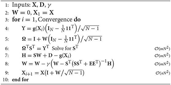
Algorithm 1. Ensemble subspace EnRML (SIES).
4. Final Algorithm
The final Subspace Iterative Ensemble Smoother (SIES) is illustrated in Algorithm 1 for the case where we represent the measurement error-covariance matrix using the ensemble of measurement perturbations. In this algorithm, the input ensembles of model states, X, and measurements D, contain all the prior information. We start by setting the initial W = 0 meaning that the input ensemble, X, is the first guess.
The most expensive computation is usually the evaluation of the forward model for the current iterate of each ensemble member to compute the predicted measurements g(Xi). This computation is at a minimum of per time step. In line 4 we subtract the mean from the predicted measurements and scale the measurement anomaly matrix by .
In line 5 we evaluate the transition matrix for the ensemble anomalies Ω, which is factorized by an LU decomposition to solve for S in line 6 to a cost 4mN2.
The “innovation” matrix H is then evaluated in line 7, where we need to compute the matrix multiplication SW at a cost mN2, and we again use the model prediction g(Xi).
We compute the next estimate of W using the iteration in line 8, where we can compute the inversion using any of the schemes discussed in section 3. However, the most efficient scheme for the case with correlated measurement errors is the one described in section 3.4.
With the updated W from line 8 we can compute the new estimate for Xi+1 in line 9 at a cost of nN2.
Algorithm 1 is truly linear in the number of measurements as well as the dimension of the state vector and provides a mean for efficient big-data model conditioning. We also note that there are no required SVDs or pseudo inversions of the ensemble anomaly matrix for the state vector. The update algorithm is also independent of X and A. The convergence only depends on the non-linearity of the forward model, possibly the ensemble size, the amount of independent information in the measurements, and of course the step-length γ.
4.1. Localization
It is possible to implement a scheme for local analysis, although we have not implemented this functionality yet. In reservoir models, a consistent localization is difficult because there are long-range correlations and pressure transients in the reservoir. Thus, a purely spatial localization can normally not be used. However, a localization scheme can be implemented where the state vector is split into segments, and each segment is updated based on a selected subset of measurements. In this case, we need to run several parallel updates, one for each segment and each having a different coefficient matrix Wi. These local Wi matrices will also have a column sum equal to zero. Localization allows for the overall solution to depart from the ensemble subspace, but the solution is still confined to the ensemble subspace for each localization segment.
4.2. Step Size
In the Gauss-linear case, a step length of one will give the global minimum in one iteration. However, we are solving N non-linear minimization problems, one for each realization, and we are using the same approximate model sensitivity matrix for all ensemble members. It is therefore likely that for some realizations a step length of one may lead to unphysical updates or updates giving an increased value of the cost function. We observe numerical problems in this case, and it seems to be a better strategy to use a shorter, more conservative step length for non-linear problems. We choose to use a step length that leads to a reduction of the averaged cost function and where most of the realizations will have a lower value of their respective cost function after each iteration. We have so far used a strategy where we start with a conservative value for the step length, typically γi = 0.6. If we begin with a too-long step length, which may lead to instabilities, the iterations would be restarted from the prior with a smaller step length. The step length is likely to depend on the particular case and ensemble size. Thus, the recommendation is to increase or decrease the initial guess of γi = 0.6 with increments of 0.1, until the iterations converge for all realizations.
The termination of the iterations can be based on a truncation value of the gradient, or one can use the relative change of the cost functions from one iteration to the next. For real reservoir applications, the time required per iteration can vary from hours to days, and one will always be limited in the number of iterations that can be run. Thus, a practical procedure is to manually stop the iterations when one sees that the cost functions for the realizations are “almost” identical from one iteration to the next.
4.3. Computational Cost
We have presented algorithms where the computational cost is proportional to mN2 and nN2, where N is the ensemble size, m is the number of measurements, and n is the state size. Thus, the algorithm is linear in the state size n and number of measurements m, and we typically have N ≪ m ≪ n.
Chen and Oliver [3] also introduced an approximate form of EnRML where the updates from the model mismatch term were neglected to eliminate the expensive SVD of A needed to compute A+. In SIES we have already eliminated this SVD without introducing any approximations. As such the approximate form of EnRML solves a different problem but it is not likely to be more computationally efficient than SIES, per iteration.
Each iteration in SIES and each update step in ESMDA can be computed at the same cost given that the same approximations and numerical schemes are used. Note that the SIES scheme can also be used in ESMDA, if we set the step length equal to 1.0, resample measurement perturbations in each step, and we correctly inflate Cdd and the measurement perturbations. On the other hand, ESMDA may require many more steps to converge than the number of iterations required by SIES [4].
Localization is often used to reduce the computational cost of the update steps. This will be the case with large number of measurements in schemes where the Kalman-gain matrix is explicitly computed to a cost proportional to m2. Localization will in SIES lead to an increase in the computational cost when we use the exact inversion with a diagonal Cdd, or when we use the approximate subspace inversion where Cdd is represented by measurement perturbations. In these two cases, the inversion is linear in the number of measurements, and solving many small problems becomes more expensive than solving one large problem. Also, the algorithm is independent of the state size except for in the final update equation, and the cost of the final update equation is the same with or without localization.
5. Verification Experiments
We will now show results from three vastly different experiments to verify the robustness of the new subspace EnRML scheme. The first model is a non-linear scalar case with one unknown and one measurement where we can compute the theoretical solution of Bayes theorem. Then, using a vast ensemble size, we can examine the convergence of the probability density functions in the limit of infinite ensemble size. For this case, we used a separate and more straightforward implementation of the algorithm.
The second case is slightly more complicated than the scalar case with a state size of three and five measurements, and using the full implementation in the Ensemble Reservoir Tool (ERT). This model resembles polynomial curve fitting, and we currently use it for extensive testing of the ERT code. Finally, we run ERT for a full history-matching case with a synthetic reservoir model.
In the following, we will use the notation ES for Ensemble Smoother and IES for the iterative ensemble smoothers where we compute the gradient of the cost function with respect to the state vector. For the subspace implementation of IES, we use SIES. Additionally, we refer to one case where we run the ensemble smoother with multiple data assimilation (ESMDA).
5.1. Scalar Case With Large Ensemble Size
A first experiment is the scalar case of Evensen [4] where we use an immense ensemble size to examine the convergence of the SIES scheme in the limit of infinite ensemble size. The scalar model is:
where, in the linear case β = 0.0 and in the non-linear case β = 0.2. We sample the prior ensemble for x from and we define the likelihood for the measurement d of the prediction y as . Thus, we run a case with state dimension equal to one and condition on a single measurement. The ensemble size is 40,000 realizations for both the SIES and the original IES methods, and the initial ensembles are identical in both cases. The IES scheme used a Gauss-Newton iteration as given in Evensen [5, section 5.2] but with model errors set to zero. Additionally, we ran an original IES case where we used 107 realizations to examine the limiting behavior of the IES scheme with practically zero sampling errors. Note that, we have designed the SIES for efficiency in the case with an ensemble size smaller than the state size, and the required storage of W ∈ ℜN×N poses a constraint for large ensemble sizes.
Since we are running both ES and IES, it is useful to see the difference between the methods in how they attempt to minimize the ensemble of cost functions in Equation (10). In the upper plot of Figure 1, we show the cost functions of five realizations in a linear scalar case. The full line shows the ES step from the prior estimate to the global minimum while the dashed lines are the corresponding IES iterative solution. In this linear case, both ES and IES converge to the same result. In the lower plot, we use a non-linear model and observe that in this case, ES is giving a poorer estimate of the global minimum than we get from the IES. Note also that IES does not solve for the exact minimum since we introduced the averaged model sensitivity instead of using the exact tangent-linear model in Equation (23).
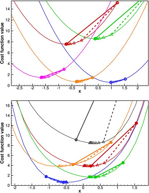
Figure 1. Examples of IES cost functions in the linear (upper plot) and non-linear (lower plot) cases. The full straight lines are the ES updates from the prior value to the estimated solution for each realization. The dashed lines show the IES steps. The ES and IES solutions are identical in the linear case and finds the global minimum. In the non-linear case IES gives an approximate estimate for the minimum that outperforms ES.
The results are shown in Figure 2 for the linear and non-linear scalar cases. In both the linear and non-linear cases, the IES and SIES results are identical, realization per realization. In the linear case, the IES with 107 realizations converges to the Bayesian posterior and so would SIES if we could run with a large enough ensemble size. In the non-linear case, IES and the SIES with equal initial ensemble and ensemble size again converge precisely to the same distribution. However, the methods do not correctly sample the posterior in the non-linear case as was pointed out by Oliver et al. [9], but see also the more recent discussions in Bardsley et al. [17], Liu et al. [18], and Evensen [4]. The minimization of the ensemble of cost functions, even if solved correctly does not accurately sample the posterior Bayes'. There is also an additional approximation introduced by using an ensemble-averaged model sensitivity. These results prove the consistency of the SIES formulation and that it exactly replicates the solution of the original IES method.
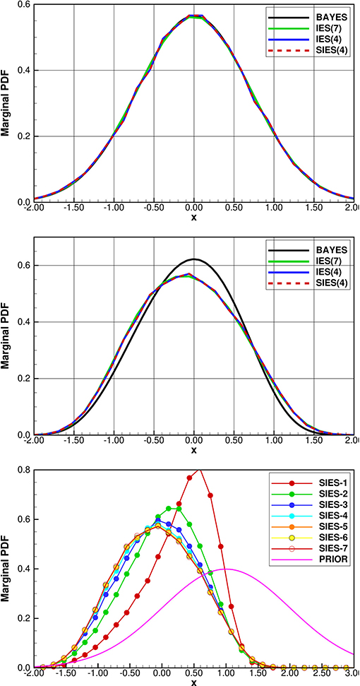
Figure 2. Scalar model: IES and SIES solutions in the linear case (upper plot) and non-linear case (middle plot). The same random seed is used in all experiments. The black pdf is the theoretical solution defined by Bayes'. The green pdf, denoted IES(7) is the converged IES solution using 107 realizations. The blue pdf denoted IES(4) is the IES solution using with 40,000 realizations, and it is exactly equal to the red dashed pdf denoted SIES(4), which is the SIES with 40,000 realizations. The lower plot shows SIES iterations in the non-linear case using 40,000 realizations. After 6 iterations the pdfs are indistinguisable.
In the bottom plot in Figure 2, we show the convergence per iteration for the scalar example. After about six iterations it is practically not possible to distinguish the distributions from one iteration to the next.
As will be illustrated below, for the SIES method, we can extrapolate this convergence rate to higher-dimensional problems since the algorithm does not depend on the state dimension. The only factors that influence the convergence of the SIES algorithm are the non-linearity of the model, the ensemble size, possibly the measurement configuration, and the step-length scheme. The code used for these examples is available from Github at https://github.com/geirev/scalar.
5.2. Verification on ERT Poly Case
We have implemented the SIES method for operational history matching where we condition reservoir models on various dynamic data. The implementation is written in C and is available from the libres library at Github https://github.com/equinor/libres, used in the Ensemble Reservoir Tool https://github.com/equinor/ert. The implementation is configured to handle the conditioning on big-data with correlated errors, and the potential loss of observations or realizations from one iteration to the next. The handling of big data is becoming increasingly important since reservoir models are now being conditioned on big seismic data sets with correlated errors, and there is a need for algorithms that scale linearly in the number of measurements (such as the ensemble-subspace algorithm discussed in section 3.4).
A loss of observations from one iteration to the next might arise because there is a filter operating on the measurements in each iteration to exclude outlier observations. This algorithm depends on the standard deviation of the ensemble, which changes in each iteration. This issue is relatively easy to handle, by keeping track of which observations are lost from one iteration to the next, and by removing the corresponding rows in the matrices.
A loss of ensemble members might typically happen because of unstable computational clusters where some nodes may crash, or a model realization may have an unstable configuration that leads to divergence and the model crashes. The approach for handling the loss of realizations is to keep track of which realizations are active and to remove the rows and columns in the W matrix corresponding to inactive realizations. The algorithm is configured to converge to the ES solution with the same active realizations in a Gauss-linear case.
The implementation in libres follows a test-based implementation, where several tests are implemented to check the consistency of the code. Several tests are run using a simple example with the following “linear” model:
Here the coefficients a, b, and c are random variables, while y(x) is evaluated at x = 0, 2, 4, 6, 8, to create the predicted measurements d1 = y(0), d2 = y(2), d3 = y(4), d4 = y(6) and d5 = y(8). Thus, we are computing polynomial curve fitting to the 5 data points. In the case with a, b, and c sampled from a normal distribution, this model comprises a Gauss-linear problem which is solved correctly by the ES, and where the ES and SIES solution becomes identical. If we sample a, b, and c from a non-normal distribution, ERT handles this by defining underlying normal distributions that through a non-linear transformation results in the specified non-normal distribution (e.g., starting from a Gaussian sample the inverse Box-Muller transformation will result in uniform samples). Thus, the same polynomial case can be made non-linear by using, e.g., uniformly distributed ensembles for a, b, and c.
We show an example of the estimated parameters of a, b, and c, in the upper, middle, and lower plots in Figure 3. The blue circles (case INI) are the prior ensembles for a, b, and c, the green circles (ES) are estimated values using the original Ensemble Smoother scheme in ERT, the red circles (SIES1.0) are estimated values from the SIES scheme using one iteration with step length one, and finally, we show the seven first iterations using SIES with a step length of 0.5. From these plots, the different schemes seem to provide the same solution as is expected, and the convergence of the SIES iterations is quite fast.
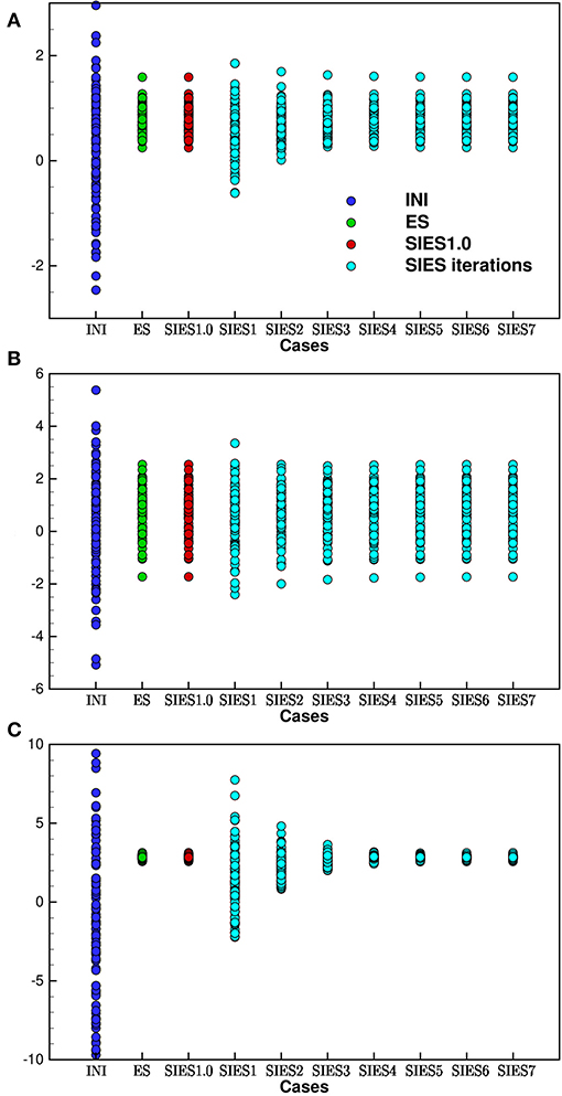
Figure 3. Coefficients a, b, and c for the polynomial Gauss-linear case: The solution using ES and SIES in the Gauss-linear case should all be identical realization per realization. The dark blue circles are the realizations of the initial ensemble. The green circles are the original ES in ERT, which are identical to the SIES scheme with a single iteration of step-length equal to 1.0 (denoted SIES1.0) shown as the red circles. The cyan circles denote iteration steps using SIES with a step length of 0.5, which also converges exactly to the ES solution.
In Figure 4, where we cross plot the estimated coefficients a and b in the upper plot and a and c in the lower plot, for the ES and SIES. It is clear that the results from SIES, the original ES scheme, and SIES with a step length of one and one single iteration (SIES1.0) all give identical results realization per realization. Also, in this linear case, we can continue iterating the IES scheme with step length one, and the solution is unchanged. This experiment is a first verification test of the new algorithm showing that the results are the same to within numerical truncation errors.
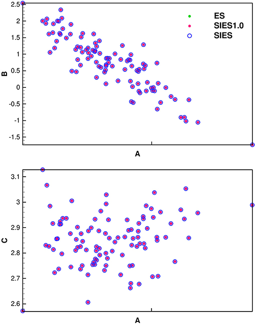
Figure 4. SIES verification using cross plots of coefficients a, b, and c for the polynomial Gauss-linear case. The solution using Ensemble Smoother (ES) and SIES with step length 1.0 (SIES1.0) are identical for each realization. The SIES converges to the ES solution as well (the result is shown after 12 iterations).
In Figure 5, we repeat the plots in Figure 4 but for ESMDA. ESMDA will lead to different results than SIES if we compare individual realizations. However, ESMDA should in the Gauss-linear case converge to the same mean and standard deviation as ES over many repeated experiments. From the plots, it appears that the ESMDA gives a result that is statistically consistent with the ES solution.
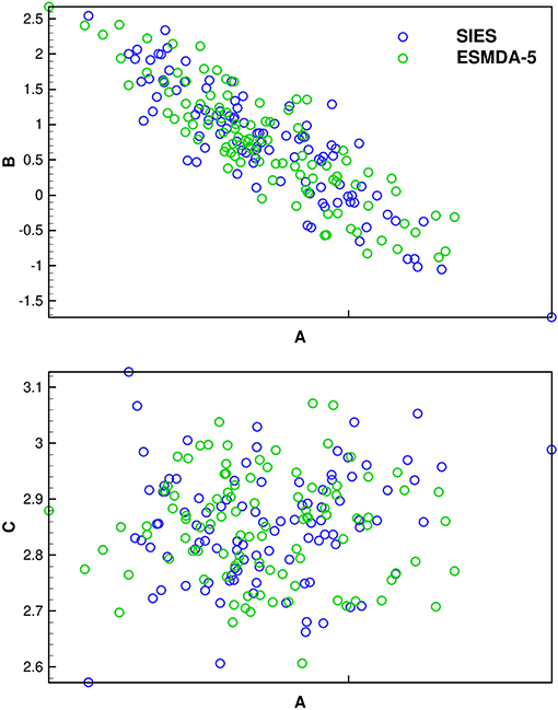
Figure 5. Cross plots of coefficients a, b, and c for the polynomial Gauss-linear case: The solution using ESMDA (here with 5 steps) differs from the SIES for each realization due to resampling of measurement errors in each ESMDA step, but the methods sample the same posterior in the Gauss-linear case.
It is difficult to verify the numerical implementation of advanced methods in applications with full reservoir models where we do not know the correct result. One would observe that different methods give different results but it is impossible to know which one is correct. These examples demonstrates the usefulness of introducing simple tests for verification of the algorithms.
5.3. Verification on a Reservoir Case
The next verification considers a relatively simple synthetic reservoir model with 27755 active grid cells on a 40-times-64 grid with 14 layers. The uncertain parameters include the three-dimensional porosity field and six fault multipliers F2–F7. There are five producing wells, OP1–OP5 and three injectors I1–I3. As the model is a simplification of a real reservoir model, it provides a reasonably realistic reservoir case. We will not describe the model at length here but rather focus on the properties of the SIES when used for parameter estimation in a reservoir case. In these cases we used a step-length scheme where for the three first iterations the step length is 0.6, then for the next three iterations it is reduced to 0.3, for subsequent iterations it is further reduced to 0.15.
In Figure 6 we show in the upper plot, the ensemble of cost functions for the experiment with exact inversion using Equation (51). We see that the first iteration significantly reduces all cost functions from their initial values. The second iteration reduces most of the cost functions, but a few also increase. However, in the subsequent iterations, all cost functions reduce their value. We decided to use a long step length while ensuring that almost all cost functions reduce their values after each update. The algorithm converges quickly, and for engineering applications, about five to six iterations should suffice to reach acceptable convergence.
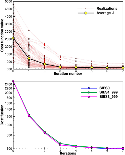
Figure 6. The upper plot shows the values of the individual cost functions for each ensemble member as a function of iterations. The lower plot shows three average cost functions (averaged over the ensemble of cost functions) for the three versions of the inversion schemes. See section 5.3 for explanation of the different cases. The subspace schemes used a truncation at 99.9% of the variance.
In the lower plot in Figure 6 we used three different inversion schemes to compute the update. We used the exact inversion from Equation (51) where it is implicitly assumed that Cdd = I (denoted as SIES0), the subspace inversion from section 3.3 with Cdd = I exactly prescribed (denoted by SIES1) and finally the subspace inversion scheme from section 3.4 with (denoted by SIES3) which introduces an approximation due to the limited ensemble size of 100 members. In both the subspace schemes, we used a truncation where we retained 99.9% of the spectrum when computing the singular value decomposition of S. From the plot we see that SIES0 and SIES1 give almost identical results, the only difference is due to the use of the truncation of some singular values, since with a diagonal Cdd the subspace scheme does not introduce any additional approximation. The approximation in the SIES3, where we represent Cdd by the measurement perturbations E, results in a small but visible difference in the cost function.
In Figure 7, we plot the ensembles of fault multipliers for the six faults in the model, as computed by the three schemes SIES0, SIES1, and SIES3. All three inversion schemes give similar results, and there would be no reason to prefer one particular approach based on these results. We see that the faults F2 and F7 retains a more substantial variance while we should probably close the faults F3 to F6.
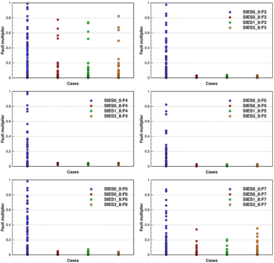
Figure 7. Reservoir case: the plots show the initial and estimated fault multipliers (after 8 iterations) for the six faults F2–F7, using the three different inversion schemes (for the plot of F2, we conveniently removed the figure legend). These plots show consistency between the different inversion schemes. The results are slightly different but qualitatively the same. See section 5.3 for explanation of the three different inversion schemes used.
In Figure 8 we show the ensembles of prior and posterior oil rates for two wells OP3 and OP5, where we used the exact inversion SIES0 and the subspace inversion SIES3 in the upper and lower plots, respectively. The results indicate that the estimation of parameters leads to a posterior ensemble that matches the observations well, without under-estimating the variance. Note, also that there is almost no visual difference between the results in the upper and lower plots.
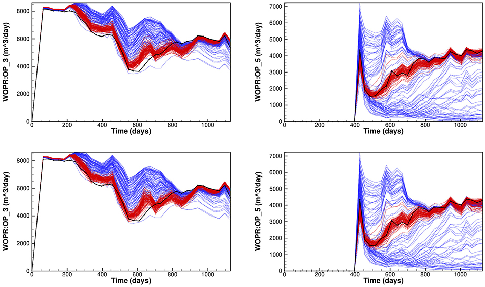
Figure 8. Reservoir case: The plots show oilrates from two different wells OP3 (left plots) and OP5 (right plots) using the exact inversion (upper plots) and the subspace inversion with .
These experiments serve as a first verification of the subspace schemes when history matching a non-linear reservoir model. The current experiments use a diagonal measurement error-covariance matrix, and we could not examine the schemes with correlated measurement errors. We will carry out more extensive such comparisons in a future publication, where the focus is on the impact of assimilating data with correlated errors. For now, Evensen [16] compared the inversion schemes for data assimilation in a linear advection equation, with correlated measurement errors, and in those cases, the results were consistent and similar using the different inversion schemes.
A final note is that the number of significant singular values in the subspace schemes decreased from 38 in the first iteration to 15 in iteration eight when we used a truncation of 0.999. In experiments with a truncation of 0.99, the corresponding decrease went from 15 to 5 significant singular values. The number of active observations was 452. This result is a clear indication of substantial redundancy in the rate data, as was discussed in more detail in Evensen and Eikrem [19].
6. Summary
We have discussed the derivation and implementation of the recently proposed subspace EnRML method by Raanes et al. [1] for practical use in reservoir history matching. We have tried to provide a complete and easy to follow sequential derivation from the fundamental Bayesian formulation to the final implemented algorithm. We include discussions on practical choices of numerical methods that lead to an efficient implementation capable of handling big datasets. In particular, the use of subspace inversion methods allows for processing of extensive data sets also in the case with correlated measurement errors. We have used a test-driven development strategy and present several examples where the numerical algorithms are run on simple examples with known solutions to verify both the theoretical fundament of the methods and the actual coding of the algorithm. Finally, we have tested our implementation in publically available software for ensemble modeling and history matching of reservoir models, Ensemble Reservoir Tool (ERT). All in all, this paper should serve as a useful guide for anyone implementing an iterative ensemble data-assimilation algorithm for operational use.
Data Availability Statement
The datasets generated for this study are available on request to the corresponding author.
Author Contributions
GE has performed most of the implementation work, including much of the programming, running of cases, and the writing of the manuscript. PR and AS have worked together with Geir Evensen on the formulation of the iterative smoother Raanes et al. [1] and contributed with theoretical discussions during the implementation and applications on the presented examples. JH was the leading developer of ERT and has contributed with advice and support, in addition to customization of ERT to accommodate the new iterative smoother method, during the practical implementation. He has also developed most of the tests, and the poly example used.
Funding
This work was supported by the Research Council of Norway and the companies AkerBP, Wintershall–DEA, Vår Energy, Petrobras, Equinor, Lundin and Neptune Energy, through the Petromaks–2 project DIGIRES (280473) (http://digires.no) and additionally by Equinor in a separate project.
Conflict of Interest Statement
JH was self-employed by company Datagr http://datagr.no.
The remaining authors declare that the research was conducted in the absence of any commercial or financial relationships that could be construed as a potential conflict of interest.
The handling editor declared a past collaboration with one of the authors PR and GE.
References
1. Raanes PN, Stordal AS, Evensen G. Revising the stochastic iterative ensemble smoother. Nonlinear Process Geophys Discuss. (2019) 2019:1–22. doi: 10.5194/npg-2019-10
2. Chen Y, Oliver DS. Ensemble randomized maximum likelihood method as an iterative ensemble smoother. Math Geosci. (2012) 44:1–26. doi: 10.1007/s11004-011-9376-z
3. Chen Y, Oliver DS. Levenberg-Marquardt forms of the iterative ensemble smoother for efficient history matching and uncertainty quantification. Computat Geosci. (2013) 17:689–703. doi: 10.1007/s10596-013-9351-5
4. Evensen G. Analysis of iterative ensemble smoothers for solving inverse problems. Computat Geosci. (2018) 22:885–908. doi: 10.1007/s10596-018-9731-y
5. Evensen G. Accounting for model errors in iterative ensemble smoothers. Computat Geosci. (2019) 23:761–75. doi: 10.1007/s10596-019-9819-z
6. Emerick AA, Reynolds AC. Ensemble smoother with multiple data assimilation. Comput Geosci. (2013) 55:3–15. doi: 10.1016/j.cageo.2012.03.011
7. Skjervheim JA, Hanea R, Evensen G. Fast model update coupled to an ensemble based closed loop reservoir management. EAGE Petrol Geostat. (2015) 5:7–11. doi: 10.3997/2214-4609.201413629
8. Hanea R, Evensen G, Hustoft L, Ek T, Chitu A, Wilschut F. Reservoir management under geological uncertainty using fast model update. In: SPE Reservoir Simulation Symposium. Houston, TX: Society of Petroleum Engineers (2015). p. 12. doi: 10.2118/173305-MS
9. Oliver DS, He N, Reynolds AC. Conditioning permeability fields to pressure data. In: ECMOR V-5th European Conference on the Mathematics of Oil Recovery. Leoben (1996). p. 11. doi: 10.3997/2214-4609.201406884
10. Kitanidis PK. Quasi-linear geostatistical therory for inversing. Water Resources Res. (1995) 31:2411–9.
11. Hunt BR, Kostelich EJ, Szunyogh I. Efficient data assimilation for spatiotemporal chaos: a local ensemble transform Kalman filter. Physica D. (2007) 230:112–26. doi: 10.1016/j.physd.2006.11.008
12. Bocquet M, Raanes PN, Hannart A. Expanding the validity of the ensemble Kalman filter without the intrinsic need for inflation. Nonlinear Process Geophys. (2015) 22:645–62. doi: 10.5194/npg-22-645-2015
13. Sakov P, Oliver DS, Bertino L. An iterative EnKF for strongly nonlinear systems. Mon Weather Rev. (2012) 140:1988–2004. doi: 10.1175/MWR-D-11-00176.1
14. Golub GH, Van Loan CF. Matrix Computations. Johns Hopkins Studies in the Mathematical Sciences, 4th Edn. Baltimore, MD: Johns Hopkins University Press (2013).
15. Evensen G. Sampling strategies and square root analysis schemes for the EnKF. Ocean Dynamics. (2004) 54:539–60. doi: 10.1007/s10236-004-0099-2
16. Evensen G. Data Assimilation: The Ensemble Kalman Filter. 2nd Edn. Berlin; Heidelberg: Springer-Verlag (2009). p. 320.
17. Bardsley J, Solonen A, Haario H, Laine M. Randomize-then-optimize: a method for sampling from posterior distributions in nonlinear inverse problems. SIAM J Sci Comput. (2014) 36:1895–910. doi: 10.1137/140964023
18. Liu Y, Haussaire J, Bocquet M, Roustan Y, Saunier O, Mathieu A. Uncertainty quantification of pollutant source retrieval: comparison of bayesian methods with application to the chernobyl and fukushima daiichi accidental releases of radionuclides. Quat J R Meteorol Soc. (2014) 143:2886–901. doi: 10.1002/qj.3138
Keywords: EnRML, iterative ensemble smoother, history matching, data assimilation, inverse methods, parameter estimation
Citation: Evensen G, Raanes PN, Stordal AS and Hove J (2019) Efficient Implementation of an Iterative Ensemble Smoother for Data Assimilation and Reservoir History Matching. Front. Appl. Math. Stat. 5:47. doi: 10.3389/fams.2019.00047
Received: 01 July 2019; Accepted: 10 September 2019;
Published: 04 October 2019.
Edited by:
Marc Bocquet, École des ponts ParisTech (ENPC), FranceCopyright © 2019 Evensen, Raanes, Stordal and Hove. This is an open-access article distributed under the terms of the Creative Commons Attribution License (CC BY). The use, distribution or reproduction in other forums is permitted, provided the original author(s) and the copyright owner(s) are credited and that the original publication in this journal is cited, in accordance with accepted academic practice. No use, distribution or reproduction is permitted which does not comply with these terms.
*Correspondence: Geir Evensen, geev@norceresearch.no