Climate Risk Assessment under Uncertainty: An Application to Main European Coastal Cities

Introduction

Sea-level rise (SLR) is a major threat to coastal areas across the world as a much of the world's population and socio-economic infrastructures are concentrated precisely in those areas (Revi et al., 2014). Low elevation coastal zones (LECZ) comprise the strip with elevations lower than 10 m above sea level. Such areas account for only 2% of the world's land, but they contain 10% of the global population. About two thirds of mega-cities with populations above 5 million people are located in low lying coastal areas and the population at risk from 100-year-return-period coastal extreme events has increased by 95% in the last 40 years (McGranahan et al., 2007). As a result, global damage associated with coastal flooding is expected to increase, not only due to the global rise in sea level, but also due to the increase in the number and the value of assets at risk (Wong et al., 2014). Urban areas can therefore be considered one of the main “hotspots of coastal vulnerability” (Newton and Weichselgartner, 2014, p. 125).

Being so vulnerable to the impacts of climate change, coastal cities have a major role in adapting to them. In this effort, one important way to enhance resilience and reduce vulnerability is to integrate the concept of risk (and therefore risk management) into regional and local decision-making processes (Newton and Weichselgartner, 2014).

The literature on disaster risk management that assesses the impacts of extreme events is vast, and can provide relevant information to local policy and decision-makers. However, when addressing climate change related issues, uncertainty is one of the main difficulties that need to be dealt with. The traditional framework for estimating flood risk damage is most commonly based on providing annual average losses obtained in a deterministic way, and of course not accounting for uncertainty. Innovative decision support tools that can help deal with uncertainty are thus required (Watkiss et al., 2015). There are other studies that have taken uncertainty into account: For example Boettle et al. (2013, 2016) use Extreme Value Theory (EVT) to assess coastal extremes in two Danish cities -Copenhagen and Kalundborg.

In this paper we propose two methods for incorporating uncertainty in the context of adaptation to climate change. The first consists of defining a stochastic process for estimating changes in sea level, in this case for the worst case emission scenario posited by the Intergovernmental Panel on Climate Change (IPPC), i.e., representative concentration pathway (RCP) 8.5, from 2010 to the end of the century. Uncertainty is also accounted for by including volatility in the probability distribution of SLR. We apply this development to data on 19 European major coastal cities for which relative SLR distributions were available (Kopp et al., 2014).

The second method consists of estimating two risk measures, namely Value-at-Risk (VaR) and Expected Shortfall (ES). Risk measure approaches have long been used in economics to effectively account for uncertainty in many variables (such as prices) by adding stochastic behavior to deterministic formulations. The VaR and ES are well-established measures in financial economics (Wilmott, 2000; Hull, 2012). This approach, used in other fields (Abadie and Chamorro, 2013; Abadie and Galarraga, 2015), is adapted and applied to the field of climate change economics in this paper. It is only recently that this approach has begun to be used in the assessment of climate risk, though both measures are very suitable in the field of the economics of adaptation, where they can provide new ways to deal with so-called tail events, i.e., low-probability, high-impact events.

Hence, the objectives of this paper are as follows: (i) to apply a method that enables uncertainty to be accounted for in future SLR outcomes for each European city under analysis; and (ii) to estimate the risk of damage for each city under the most extreme SLR scenario (RCP8.5) for different time periods. This information can be used for instance, to define acceptable levels of risk for each city. Awareness of the magnitude and timing of risk is a key element for defining how much adaptation is needed and by when it needs to be put into practice.

The main contribution of our study is the calibration of a stochastic diffusion model with regionalized SLR for each city. We obtain the expected damage for every year from the baseline to 2100 as well as two risk measures, namely the VaR and the ES, with the latter being especially important. We believe that this study can provide guidance for coastal managers and policy makers in dealing better with coastal extreme events (“tail events”; Hinkel et al., 2015).

Methods

This paper has two main parts: first it calibrates a stochastic diffusion model using regionalized IPCC data. That calibration provides a probability distribution of SLR at any time between the baseline and the end of the period considered (2100). As the aim of this study is not to measure expected damage but the impact of the worst 5% of cases, secondly we measure risk through two methodologies: the first is the value at risk (VaR), which reveals that only in 5% of cases will a certain level of damage be exceeded. The VaR therefore shows when the tail of the worst cases starts, but it does not tell us any more about that tail. In spite of its widespread use, the VaR does not have the best properties for assessing risk (see for example, Hull, 2012). This is why we also use the Expected Shortfall (ES) as a more relevant risk measure. The ES represents the average damage in the worst cases (in our study, the worst 5%). Although we consider ES a much more appropriate risk measure, we also consider the VaR as it is a standard measure which is widely used in financial economics.

Future Projections of Sea-Level Rise at City Level

Global sea-level has risen by more than 20 cm since 1980 (Hardy and Nuse, 2016) and the rate of SLR during the twentieth century is estimated to have been 1.7 ± 0.3 mm year⁻¹ (Church and White, 2006, p. 2). However, recent estimates measured via satellite altimetry show an acceleration range of 2.6–2.9 ± 0.4 mm year⁻¹ for the period between 1993 and mid-2014 (Watson et al., 2015).

Deciding on how much adaptation to climate change is needed at local scale and when to implement it requires detailed information on future risks. The latest IPCC projections of mean global sea-level changes (Church et al., 2013), the so-called Representative Concentration Pathways (RCPs), do not provide the level of information required for local and regional policies. There is clear evidence of global SLR as a result of climate change (Church et al., 2013) but the relative sea level varies widely on a local and regional basis (Stammer et al., 2013). Relative sea level represents the actual relationship between the ocean surface and the land, and it depends on several factors: (i) eustatic determinants, i.e., absolute changes in sea level as a result, for example, of thermal expansion or ice melting (Lambeck et al., 2010); (ii) static equilibrium effects, defined as “perturbations in the Earth's gravitational field and crustal height associated with the redistribution of mass between the cryosphere and the ocean” (Kopp et al., 2014: 383); (iii) glacial isostatic adjustment, which causes the uplift of land in the areas affected by ice-caps during the last glaciation (Simon et al., 2016); (iv) vertical land uplift resulting from other local processes such as tectonism or subsidence due to groundwater depletion or sediment compaction (Miller et al., 2013; Kopp et al., 2014).

A comprehensive dataset of local sea-level projections was developed by Kopp et al. (2014) for a worldwide network of tide-gage sites. The projections in that dataset consider the following factors that contribute to changes in sea level: (i) three ice-sheet components; (ii) glacier and ice caps; (iii) surface mass balance; (iv) oceanographic processes; (v) land water storage; and (vi) other long-term local non-climatic factors such as glacial isostasy, tectonics, and sediment compaction.

Another limitation of the IPCC projections is that only likely probability ranges are given (i.e., 66–100% probability ranges), so low-probability, high-damage events are left out. Of course, this makes it very difficult to assess tail events.

However, for coastal cities Kopp et al. (2014) provide the full probability distribution for each site, which enables us to focus on the worst cases and estimate the risk for the major coastal cities in Europe. We use the 2030, 2050 and 2100 medians and the 95 percentile in 2100 from Kopp et al. (2014) for 19 European cities (see Table 1) to calibrate a stochastic diffusion model that enables us to estimate the change in sea-level for each city at any given point in time up to the year 2100.

TABLE 1

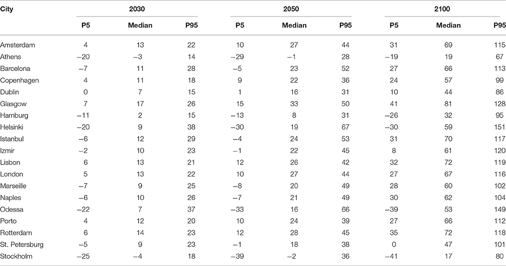
Table 1. Future sea-level rise projections for each city under RCP8.5, measured in cm. Source: Kopp et al. (2014).

Note that the concept of risk used in this paper focuses on the probability of occurrence of the worst cases, so we are only considering the most extreme SLR scenario (RCP8.5), which is a business as usual scenario (Grinsted et al., 2015)¹.

A Continuous Stochastic Diffusion Model for Local Sea-Level Rise

We now apply the Geometric Brownian Motion stochastic process (GBM) (Wilmott, 2000; Hull, 2012; Abadie and Chamorro, 2013) to estimate the changes in sea level for each city k, as defined in Equation (1):

$\begin{array}{ll}d{V}_t^k={\alpha }^k{V}_t^{k}dt+{\sigma }^k{V}_t^{k}d{W}_t^k& (1)\end{array}$

where $V_t^k$ represents the SLR of city k at time t, plus an initial value $V_0^k$. This current value grows at rate α^k; the term σ^k is the instantaneous volatility, and $d{W}_t^k$ denotes the increment to a standard Wiener process. The initial value $V_0^k$ is used to ensure a better fit of the modeling of the RCP8.5 scenario of each city. This is only a scale change.

Equation (1) represents a standard Brownian motion model in which a change in a variable V of city k at time t occurs as a result of two elements (two addends):

1. A determinist addend in which α^k represents the exponential tendency of the expected value (see Equation 2).

2. A stochastic addend where the volatility σ^k determines the level of uncertainty.

Geometric Brownian motion is a standard stochastic diffusion model in financial economics and has well-known properties. As we are applying a stochastic diffusion model to represent SLR uncertainty, we selected this model for its simplicity, the small number of parameters that is uses, and its characteristics. One of its main features is that its value grows exponentially, which adapts to IPCC scenarios, where the value is expected to behave in this way. This makes for a better calibration².

One of the characteristics of this model is that it does not generate negative values, so $V_t^k>0$ at all times. For this reason, the initial value $V_0^k$ must be different from zero, otherwise we would always obtain $d{V}_t^k=0$. This limitation can be solved by using a base level $V_0^k$ placed below current sea level whose value is calculated optimally. Thus, the effective SLR at time t $S_t^k$ is estimated as the difference between $V_t^k$ and $V_0^k$. $S_t^k=V_t^k-V_0^k$.

At a time t this distribution process generates a log-normal distribution where the first moment (mean) is defined by Equation (2):

$\begin{array}{rc}E(V_t^k)=V_0^k{e}^{{\alpha }^{k}t}& (2)\end{array}$

And the median is defined by Equation (3):

$\begin{array}{ll}median(V_t^k)=V_0^k{e}^{(({\alpha }^k-{({\sigma }^k)}^2)t}& (3)\end{array}$

The variance is expressed by Equation (4):

$\begin{array}{rc}Var(V_t^k)={(V_0^k)}^2{e}^{2{\alpha }^{k}t}\left(e^{{({\sigma }^k)}^{2}t}-1\right)& (4)\end{array}$

If we now define $X_t^k=ln{V}_t^k$ then $X_t^k$ follows a normal distribution with the moments defined by Equations (5)–(7):

$\begin{array}{rc}E(X_t^k)=X_0^k+\left({\alpha }^k-\frac{{\sigma }_V^2}{2}\right)t& (5)\end{array}$

$\begin{array}{rc}Var(X_t)={({\sigma }^k)}^{2}t& (6)\end{array}$

$\begin{array}{rc}ln(V_t)~\varphi [ln(V_0)+({\alpha }^k-\frac{{({\sigma }^k)}^2}{2})t,{\sigma }_V^{2}t]& (7)\end{array}$

As mentioned, the model is calibrated using the median SLR data for 2030, 2050, and 2100 and the 95% upper percentile in 2100 presented in Table 1. The results of the calibration process are shown in Table 2.

TABLE 2

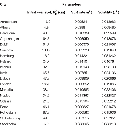
Table 2. Estimated values obtained for the different parameters in the calibration process.

These values are calculated as follows: first we obtain the value of SLR ($V_0^k$) in each city k and ${\alpha }^k-\frac{{({\sigma }^k)}^2}{2}$ in a way that meets Equation (8):

$\begin{array}{l}median(V_t^k)=V_0^k{e}^{(({\alpha }^k-{({\sigma }^k)}^2)t}=V_0^k+median(S_t^k)fort\\ =23,43,93& (8)\end{array}$

where the initial year is 2007 and thus t = 23,43,93 correspond to 2030, 2050, and 2100 respectively.

The 95% percentile calibration process is based in the following lognormal property:

$\begin{array}{rc}{\sigma }^k\sqrt{t}=\frac{\text{ln}(E{F}_t^K)}{1.645}& (9)\end{array}$

where $E{F}_t^K$ is the error factor, defined as:

$\begin{array}{rc}E{F}_t^K=\frac{95thpercentile(V_t^K)}{median(V_t^K)}& (10)\end{array}$

Equations (9) and (10) enable us to calculate the volatility σ^k of each city k. And with the volatility σ^k and the value of ${\alpha }^k-\frac{{({\sigma }^k)}^2}{2}$ calculated previously we can obtain the expected sea-level-rise growth rate α^k for each city.

Using this model, we obtain a probability distribution of SLR for each city that changes over time. Figure 1 illustrates this trend in probability for London. Observe that average values shift toward higher sea levels, but the shape of the distribution also changes.

FIGURE 1

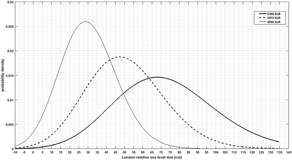
Figure 1. Probability distribution for scenario RCP 8.5 over time for London.

Estimating Risk Measures

As previously stated, the use of risk indicators such as the VaR (α) and ES (α) enables uncertainty to be accounted for by focusing on tail events. VaR (α) is the value of the loss corresponding to an SLR in the (α) percentile while ES (α) refers to the mean expected loss when the VaR is exceed. A full description of the risk measures can be found in Artzner et al. (1999) and in the Supplementary Material to this paper. In this case we have selected the 95% percentile to represent the very low-probability but high-damage events that are attracting increasing attention in the literature of climate change economics (Weitzman, 2009, 2013; Nordhaus, 2011). The rationale behind assessing these events is the huge scale of the potential damage, despite their low probability of occurrence (Pindyck, 2011).

The GBM stochastic model defined by Equation (1) is now used to generate a large number of scenarios using Monte Carlo simulation methods that enable us to calculate the risk of damage caused by SLR using the VaR (α) and the ES (α).

The first step in this process is to find a discretization algorithm which is both exact and simple, i.e., with which the differential equation can be integrated exactly; the result is as follows:

$\begin{array}{rc}{S}_t=S_0{e}^{(\alpha -\frac{{\sigma }^2}{2})t+\sigma {\displaystyle {\int }_0^t}dW}& (11)\end{array}$

Equation (11) is the solution to stochastic differential Equation (1) (see Kloeden and Platen, 1999).

Now, over a time step Δt we have:

$\begin{array}{rc}{S}_{t+\Delta t}=S_t+\Delta S=S_t{e}^{(\alpha -\frac{{\sigma }^2}{2})\Delta t+\sigma \sqrt{\Delta t}\epsilon }& (12)\end{array}$

where ΔS denotes the change in S over Δt, and ε stands for a random sample from a N(0,1) distribution. This calculation follows the method presented in Abadie and Chamorro (2013), where a Monte Carlo method is applied together with stochastic diffusion models. Equation (12) corresponds to the use of a numerical method (in this case Monte Carlo) for resolving (Equation 11).

Note that (Equation 12) does not depend on the size of Δt. Therefore, Δt need not be small. Indeed, if there is just one risk value which depends only on the terminal value of the asset then the latter can be simulated in a great leap using a time step of length T. However, there is still a minor error that can arise from using a finite number of random numbers (Abadie and Chamorro, 2013). The geometric Brownian motion has this property: formula (12) can be used for Δt = 1 and also for Δt = 20 years. In our case, using Monte Carlos simulations for Δt = 93 years and applying Equation (12), we obtain the probability distribution of SLR in 2100 for each city. Equation (12) is a property of the GBM stochastic model. In other types of stochastic process each Monte Carlo realization must usually be carried out step by step for small Δt values.

In this case we use 5,000,000 Monte Carlo simulations for the RCP8.5 scenario of each city's sea-level rise. The large number of simulations enables us to approximate almost exactly the theoretical distribution of $S_t^k$ at time t. This can be proven by finding the median and the 95th percentile of the simulated values and comparing them with the theoretical values. Using the 95th percentile we have 250,000 simulated values for the most unfavorable situations, which enables us to obtain highly accurate values of VaR (95%) and ES (95%). Any value of confidence level could be used. As stated above, in this case we consider a confidence level of 95%, which corresponds to the worst 5% of cases. Table 3 shows our simulated values for 2100 compared to those estimated by Kopp et al. (2014). Because we focus on the worst cases, the model is calibrated using the 95th percentile in 2100 and the median in 2030, 2050, and 2100. Thus, the simulated values obtained are exactly the same as those obtained by Kopp et al. (2014) for this percentile and the median, but differ slightly for the 5th percentile. With our calibration, we now have a stochastic diffusion model for each city and we can do risk calculations for any given date. The calibrated stochastic diffusion model could also be used to calculate real options.

TABLE 3

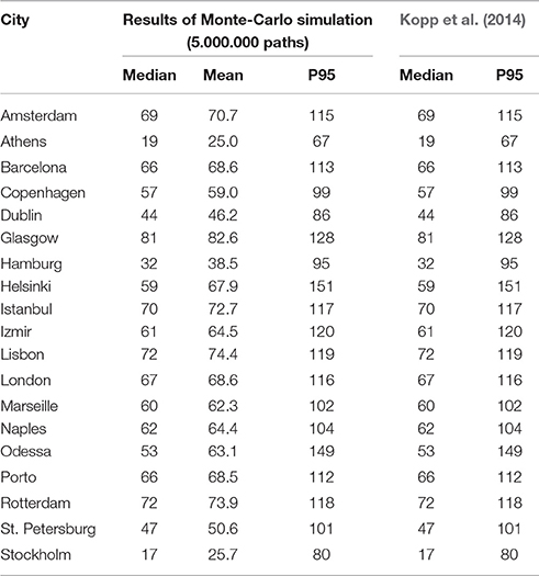
Table 3. Theoretical and simulated values of sea-level rise in 2100 (cm).

The Economic Damage Function

Once the probability distribution of SLR is obtained, the objective is now to calculate the economic losses in each city. To that end, the damage function for each city k at each time t is defined as follows:

$\begin{array}{rc}{D}^{k,t}=f(S_t^k,t)& (13)\end{array}$

At time t the function presents the following form:

$\begin{array}{rc}{D}^{k,t}=f^1(S_t^k)+f^2(t)& (14)\end{array}$

where $f^1(S_t^k)$ represents the impact of SLR at time t, while $f^2(S_t^k)$ shows the socioeconomic impacts in the absence of SLR. The additive damage specification of Equation (14) is a limitation that arises from the data available: on the one hand, we have the exposure of assets and population at risk. This exposure changes over time due to socioeconomic development. On the other hand, for each city we have an area at risk of coastal flooding that will increase due to sea-level rise. We thus assume that damage consists of the sum of the socioeconomic effect plus the damage caused by sea-level rise.

The city-specific damage function has three main components:

(i) The local SLR $S_t^k$ at time t in each city, estimated using the stochastic GBM model as described in Section Future Projections of SLR at City Level

(ii) The damage based on the population and assets at risk of coastal flooding together with the socio-economic development of each city in the future from Hallegatte et al. (2013)³. Note that as a result damage also varies in a deterministic way following future socio-economic development.

(iii) The probability of different extreme flood levels in each city. This information was obtained from our stochastic model together with the damage function from Hallegatte et al. (2013), which incorporates results from the DIVA model (Vafeidis et al., 2008) on the probability of extreme events. The effect of coastal extreme events is added to the expected SLR. Consequently, losses can happen even when flood defenses are sufficient to cope with the (mean) relative sea-level rise.

In areas where there are coastal defenses, we assume that they fail to provide any protection once they are overcome, i.e., once sea level exceeds the height of the defense infrastructure.

In this way we calibrate a continuous damage function for each city using discontinuous data. The main factor that increases damage is found to be SLR, but both factors obviously contribute to increases in risk over time.

Results and Discussion

Stochastically estimated annual average losses for main European coastal cities are shown in Table 4. Note that overall values range from US$1.2 billion in 2030 up to US$40.8 billion by the end of the century. The ranking of cities that can expect the greatest losses changes depending on the reference year. In 2030 it is led by Rotterdam, followed by Istanbul and Izmir. No loss is expected for Athens and Stockholm in 2030 because eustatic SLR is offset by other local processes. In 2050 losses in Istanbul can be expected to increase 7-fold and the Turkish city replaces Rotterdam at the head of the ranking. Losses increase significantly for all cities with respect to 2030, but the top five cities remain the same throughout the period. By the end of the century Istanbul remains as the city with the biggest losses, followed by Odessa, Izmir, and Rotterdam. For the top five cities damage is expected to increase between 4-fold and more than 7-fold with respect to 2050. Athens and Stockholm show negative expected sea-level rises in 2030, but we do not assume any benefit in this initial behavior. These values are comparable to other values in the relevant literature.

TABLE 4

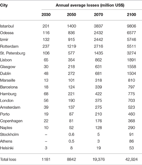
Table 4. European cities ranked by annual average losses (AAL) in 2100.

Using Monte Carlo simulations enables us to go one step further and obtain the distribution of damage for each city. For illustrative purposes, Figures 2, 3 present this damage distribution for the top 8 cities in the ranking in 2100. Observe that the horizontal axis is different in each figure and the vertical axis changes for each city.

FIGURE 2

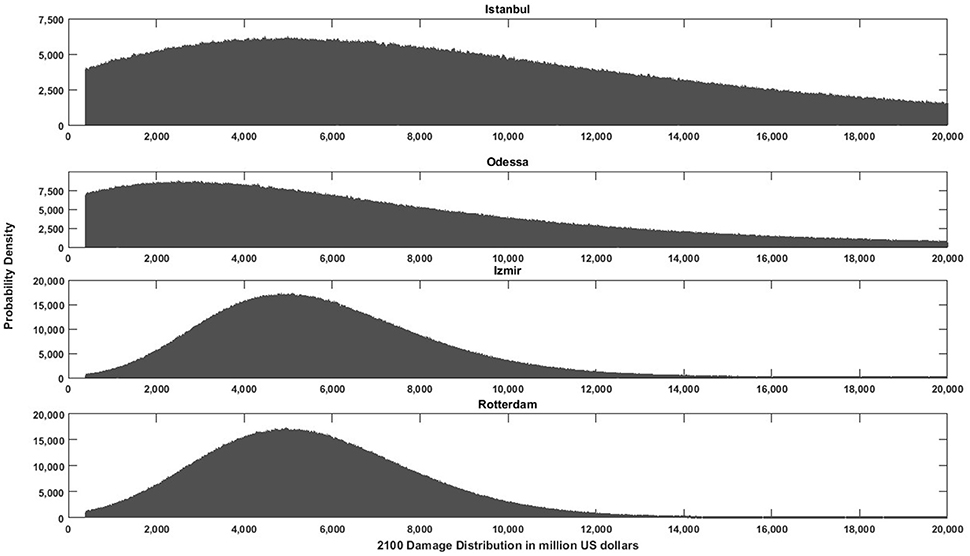
Figure 2. Damage distribution in 2100 and uncertainty distributions for the top 4 European cities under RCP8.5. Note that the vertical scale differs depending on the city.

FIGURE 3

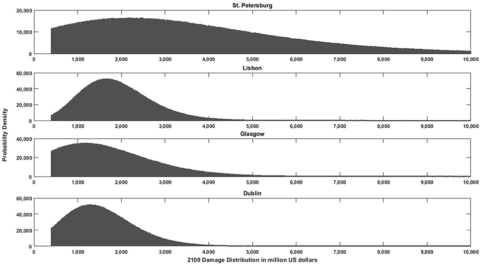
Figure 3. Damage distribution in 2100 and uncertainty distributions under RCP8.5 for the European cities ranked 4–8 in Table 4. Note that the vertical scale differs depending on the city.

Having the probability distribution of losses for different years enables us to measure risk for tail events. When attention is focused on low-probability but highly negative events through the estimation of risk measures, the results are dramatically higher than those in Table 4 (see Figure 4).

FIGURE 4

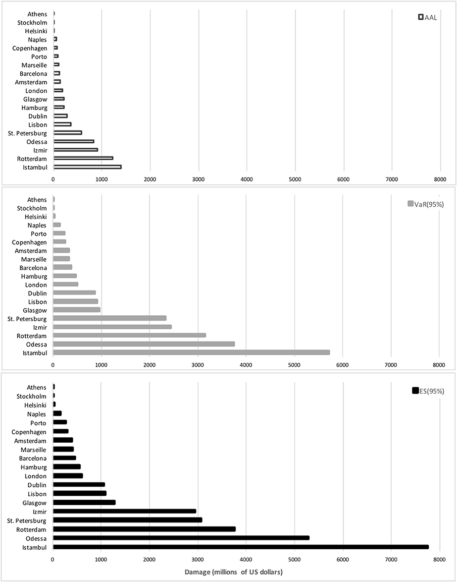
Figure 4. Risk for main European coastal cities ranked by Expected Shortfall (ES) in 2050, under RCP8.5. Damage is measured in millions of US dollars.

The VaR (95%) and ES (95%) estimated for the nineteen European cities show aggregate values of US$ 4.8 and 8.2 billion in 2030, respectively. These aggregate losses increase to US$ 92.4 and 114.8 billion in 2100⁴. The top five cities in the ranking of damage do not change when risk measures arfe considered, although the 5% of worst cases for losses in 2100 are more than double the annual average losses. The results of the VaR (95%) and ES (95%) for each city are shown in Table 5. Further results are provided in the Supplementary Material.

TABLE 5

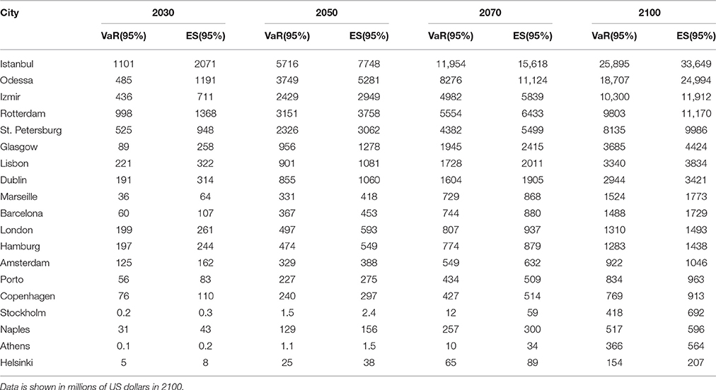
Table 5. Risk for main European coastal cities ranked by Expected Shortfall (ES).

The top five cities are the same as when the analysis focusses on annual average values but the order changes. In 2030 Istanbul is the city most at risk according to ES (95%) –that is, the mean damage for those worst 5% of cases— followed by Rotterdam and St. Petersburg. By 2050 the ranking is still led by Istanbul, but now followed by Odessa, Rotterdam, and Izmir. The Expected Shortfall in 2050 for the top cities is 4–5 times higher than in 2030. By 2100, ES (95%) is three to 7-fold the figure for 2050. By the end of the century Izmir has moved up to third place.

A comparison of the damage in the worst 5% [(i.e., ES (95%)] with the trend in each city's GDP reveals that in 2030 every city except Istanbul and London has a projected GDP lower than US$ 220 billion while ES (95%) remains below US$1.4 billion. London and Istanbul both have higher city GDPs than the rest, but the latter presents the highest risk: in excess of US$ 2 billion (Figure 5). By 2070 the relationship between risk and GDP varies: Istanbul shows the highest city GDP at over US$1200 billion, but also the highest risk at almost US$16 billion. London's GDP doubles to more than US900 billion; risk increases 3-fold but remains below US$900 billion. Risk increases 10-fold in the case of Odessa, from US$1.2 billion in 2030 to more than US$11 billion by 2070, while the city's GDP remains below US$72 billion. Following the ranking of cities with highest risk. Izmir. Rotterdam and St. Petersburg show significant increases in ES (95%) in relation to city GDP.

FIGURE 5

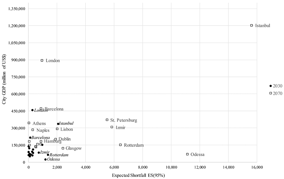
Figure 5. GDP of European cities in 2030 and 2070 vs. ES (95%). under RCP8.5.

Results under Different Probabilities for RCP8.5

The results presented so far are for RCP8.5 only, i.e., they assume a 100% probability of occurrence for this scenario. Our reason for not considering other scenarios is that we are only focusing our attention on the worst 5% of cases and most of them are found within the probability distribution of damage in the RCP8.5 scenario. In this case we perform a sensitivity analysis to see how the results change if RCP8.5 is allocated a lower-than-100% probability. Table 6 shows the results for 25% and 50% probabilities of RCP8.5 in 2050⁵. Reducing the probability of RCP8.5 lowers the risk for all cities. The top five cities in the ranking remain the same.

TABLE 6

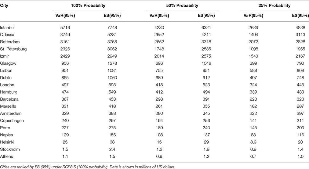
Table 6. Losses in European cities for different probabilities of occurrence of RCP8.5 in 2050.

If the same process is followed for 2100 similar results emerge: the top five in the ranking are the same, but Izmir is now third and Rotterdam drops to fourth. For Istanbul and Odessa, the risk is reduced approximately by one third (31% and 34%, respectively) when the probability of RCP8.5 is 25%. The reduction is lower for the rest of cases (see Table 7).

TABLE 7

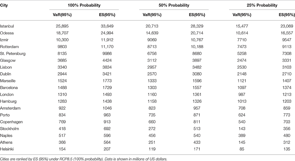
Table 7. Losses in European cities for different probabilities of occurrence of RCP8.5 in 2100.

Conclusions

In the light of potential climate damage, the economics of adaptation are currently receiving great attention, particularly those studies that can offer reliable estimates that are useful for decision making. In this paper we estimate economic losses related to SLR in coastal cities. But we do so while paying special attention to one highly relevant factor: uncertainty. This factor needs to be carefully considered when calculating economic damage but most previous studies fail to properly account for it.

We incorporate three major innovations with respect to previous studies assessing expected economic losses from coastal extreme events. The first is the use of local relative SLR projections for each city which incorporate not only eustatic sea-level but also other processes identified at each site, including site-specific probability distribution parameters as defined by Kopp et al. (2014).

The second innovation is that instead of approaching SLR deterministically we model it stochastically using a stochastic diffusion model. This modeling approach enables us to account for uncertainty and provides a diffusion model that can be used for many other calculations and at any given point in time.

The third innovation is a city-specific assessment of risk, drawn up by calculating two risk measures: (i) the VAR (95%), which represents the economic losses corresponding to the 95th percentile of the distribution of damage; and (ii) the ES (95%), which gives the average damage of the worst 5% of cases.

We believe this information to be highly relevant for decision making as it helps provide a much precise, deeper understanding of the risk faced. We acknowledge that dealing with many different sources of uncertainty is a challenging task, so innovative economic decision-support tools such as those identified by Newton and Weichselgartner (2014) and Watkiss et al. (2015) among others, are very necessary.

In this paper we have adapted methods for dealing with uncertainty that are well-known in other fields of economics (such as financial economics) and have successfully applied them to climate change adaptation in 19 European coastal cities. These methods enable us to turn our attention to so-called tail events. Our results show that despite their low probability of occurrence, the huge scale of the damage from them in comparison to annual average ones requires that they be very carefully considered in coastal vulnerability analysis. Local, regional, and national policy-makers should not settle for traditional approaches but should seek to introduce risk assessments under uncertainty into their decision-making processes. This would enable them, for instance, to define some kind of acceptable level of risk according to the actual situation of each city and the risk aversion of decision makers, which would be a key input for effectively implementing adaptation to climate change. Finally, experience shows that “disasters are improbable but they do happen,” so policy makers need to consider them (Newton and Weichselgartner, 2014, p. 131).

Risk is an important variable for policymakers who need to deal with coastal extreme events in a context of rising sea-levels and especially for risk-adverse coastal management (Hinkel et al., 2015). This paper can serve as a guide to help regional, national, and supranational policymakers in Europe deal with low-probability, high-risk coastal extreme events. Our approach reveals not only the damage under the worst 5% of cases but also the trend in damage according to the RCP 8.5 emission scenario. In line with the level of risk in each coastal city and the risk aversion of decision-makers, adaptation measures will need to be implemented in the near future in order to avoid critical damage. These decisions should take into account the time needed to adapt, i.e., investment in adaptation will have to be designed and planned long enough beforehand to avoid major losses.

Author Contributions

All authors listed, have made substantial, direct and intellectual contribution to the work, and approved it for publication.

Funding

The authors gratefully acknowledge funding from the European Union's Seventh Framework Programme for research, technological development and demonstration under grant agreement No. 603906 (Project: ECONADAPT). LMA and IG are grateful for financial support received from the Basque Government via project GIC12/177-IT-399-13. This work has also received funding from the European Union's Horizon 2020 Research and Innovation Programme under grant agreement No. H2020-DRS-9-2014 (Project: RESIN). LMA thanks the financial support from the Spanish Ministry of Science and Innovation (ECO2015-68023).

Conflict of Interest Statement

The authors declare that the research was conducted in the absence of any commercial or financial relationships that could be construed as a potential conflict of interest.

Supplementary Material

The Supplementary Material for this article can be found online at: https://www.frontiersin.org/article/10.3389/fmars.2016.00265/full#supplementary-material

Footnotes

1. ^Similarly, other RCP scenarios could be modeled but are not so interesting from the point of view of extreme events.

2. ^Other, more sophisticated stochastic models such as mean-reverting models do not show this behavior.

3. ^Two possible socio-economic scenarios are developed by Hallegatte et al. (2013): in the first the population of every city in a country grows at the same rate, and in the second scenario population growth is limited to 35 million inhabitants. The data from the second scenario is used here.

4. ^Of course, this is the case of perfect positive correlation between sea-level rise in every city. For the sake of simplicity when describing the results, we assume that if the worst scenario happens in one city it also does so in the rest.

5. ^Further results are included in the Supplementary Material.

References

Abadie, L. M., and Chamorro, J. M. (2013). Investment in Energy Assets under Uncertainty: Numerical Methods in Theory and Practice, 1st Edn. London: Springer.

Abadie, L. M., and Galarraga, I. (2015). Managing Energy Price Risk in Compendium of Energy Science and Technology, Vol 12. Houston, TX: Studium Press LLC.

Artzner, P., Delbaen, F., Eber, J.-M., and Heath, D. (1999). Coherent measures of risk. Math. Finance 9, 203–228. doi: 10.1111/1467-9965.00068

CrossRef Full Text | Google Scholar

Boettle, M., Rybski, D., and Kropp, J. P. (2013). “Adaptation to sea level rise: calculating costs and benefits for the case study Kalundborg, Denmark,” in Climate Change Adaptation in Practice: From Strategy Development to Implementation, eds P. Schmidt-Thomé and J. Klein (Chichester: John Wiley & Sons Inc), 25–34.

Boettle, M., Rybski, D., and Kropp, J. P. (2016). Quantifying the effect of sea level rise and flood defence – a point process perspective on coastal flood damage. Nat. Hazards Earth Syst. Sci. 16, 559–576. doi: 10.5194/nhess-16-559-2016

CrossRef Full Text | Google Scholar

Church, J. A., Clark, P. U., Cazenave, A., Gregory, J. M., Jevrejeva, S., Levermann, A., et al. (2013). “Sea level change,” in Climate Change 2013: The Physical Science Basis. Contribution of Working Group I to the Fifth Assessment Report of the Intergovernmental Panel on Climate Change, eds T. F. Stocker, D. Qin, G. K. Plattner, M. Tignor, S. K. Allen, J. Boschung, A. Nauels, Y. Xia, V. Bex, and P. M. Midgley (Cambridge: Cambridge University Press), 1137–1216.

Church, J. A., and White, N. J. (2006). A 20th century acceleration in global sea-level rise. Geophys. Res. Lett. 33:L01602. doi: 10.1029/2005GL024826

CrossRef Full Text | Google Scholar

Grinsted, A., Jevrejeva, S., Riva, R., and Dahl-Jensen, D. (2015). Sea level rise projections for northern Europe under RCP8.5. Clim. Res. 64, 15–23. doi: 10.3354/cr01309

CrossRef Full Text | Google Scholar

Hallegatte, S., Green, C., Nicholls, R. J., and Corfee-Morlot, J. (2013). Future flood losses in major coastal cities. Nat. Clim. Change 3, 802–806. doi: 10.1038/nclimate1979

CrossRef Full Text | Google Scholar

Hardy, R. D., and Nuse, B. L. (2016). Global sea-level rise: weighing country responsibility and risk. Clim. Change 137, 333–345. doi: 10.1007/s10584-016-1703-4

CrossRef Full Text | Google Scholar

Hinkel, J., Jaeger, C., Nicholls, R. J., Lowe, J., Renn, O., and Peijun, S. (2015). Sea-level rise scenarios and coastal risk management. Nat. Clim. Change 5, 188–190. doi: 10.1038/nclimate2505

CrossRef Full Text | Google Scholar

Hull, J. (2012). Options, Futures, and Other Derivatives, 8th Edn. Harlow: Pearson/Prentice Hall.

Kloeden, P. E., and Platen, E. (1999). Numerical Solution of Stochastic Differential Equation. Berlin: Springer.

Kopp, R. E., Horton, R. M., Little, C. M., Mitrovica, J. X., Oppenheimer, M., Rasmussen, D. J., et al. (2014). Probabilistic 21st and 22nd century sea-level projections at a global network of tide-gauge sites: KOPP ET AL. Earths Future 2, 383–406. doi: 10.1002/2014EF000239

CrossRef Full Text | Google Scholar

Lambeck, K., Woodroffe, C. D., Antonioli, F., Anzidei, M., Gehrels, W. R., Laborel, J., et al. (2010). “Paleoenvironmental records, geophysical modeling, and reconstruction of sea-level trends and variability on centennial to longer timescales,” in Understanding Sea-Level Rise and Variability, eds J. A. Church, P. L. Woodworth, T. Aarup, and S. Wilson (Chichester: Wiley-Blackwell), 61–121.

McGranahan, G., Balk, D., and Anderson, B. (2007). The rising tide: assessing the risks of climate change and human settlements in low elevation coastal zones. Environ. Urban. 19, 17–37. doi: 10.1177/0956247807076960

CrossRef Full Text | Google Scholar

Miller, K. G., Kopp, R. E., Horton, B. P., Browning, J. V., and Kemp, A. C. (2013). A geological perspective on sea-level rise and its impacts along the U.S. mid-Atlantic coast. Earths Future 1, 3–18. doi: 10.1002/2013EF000135

CrossRef Full Text | Google Scholar

Newton, A., and Weichselgartner, J. (2014). Hotspots of coastal vulnerability: A DPSIR analysis to find societal pathways and responses. Estuar. Coast. Shelf Sci. 140, 123–133. doi: 10.1016/j.ecss.2013.10.010

CrossRef Full Text | Google Scholar

Nordhaus, W. D. (2011). The economics of tail events with an application to climate change. Rev. Environ. Econ. Policy 5, 240–257. doi: 10.1093/reep/rer004

CrossRef Full Text | Google Scholar

Pindyck, R. S. (2011). Fat tails, thin tails, and climate change policy. Rev. Environ. Econ. Policy 5, 258–274. doi: 10.1093/reep/rer005

CrossRef Full Text | Google Scholar

Revi, A., Satterthwhite, D. E., Aragón-Durand, F., Corfee-Morlot, J., Kiunsi, R. B. R., Pelling, M., et al. (2014). “Urban areas,” in Climate Change 2014: Impacts, Adaptation, and Vulnerability. Part A: Global and Sectoral Aspects. Contribution of Working Group II to the Fifth Assessment Report of the Intergovernmental Panel on Climate Change, eds C. B. Field, V. R. Barros, D. J. Dokken, K. J. Mach, M. D. Mastrandrea T. E. Bilir, M. Chatterjee, K. L. Ebi, Y. O. Estrada, R. C. Genova, B. Girma, E. S. Kissel, A. N. Levy, S. MacCracken, P. R. Mastrandea, and L. L. White (Cambridge: Cambridge University Press, Cambridge) 535–612.

Simon, K. M., James, T. S., Henton, J. A., and Dyke, A. S. (2016). A glacial isostatic adjustment model for the central and northern Laurentide Ice Sheet based on relative sea level and GPS measurements. Geophys. J. Int. 205, 1618–1636. doi: 10.1093/gji/ggw103

CrossRef Full Text | Google Scholar

Stammer, D., Cazenave, A., Ponte, R. M., and Tamisiea, M. E. (2013). Causes for contemporary regional sea level changes. Annu. Rev. Mar. Sci. 5, 21–46. doi: 10.1146/annurev-marine-121211-172406

PubMed Abstract | CrossRef Full Text | Google Scholar

Vafeidis, A. T., Nicholls, R. J., McFadden, L., Tol, R. S. J., Hinkel, J., Spencer, T., et al. (2008). A new global coastal database for impact and vulnerability analysis to sea-level rise. J. Coast. Res. 917–924. doi: 10.2112/06-0725.1

CrossRef Full Text | Google Scholar

Watkiss, P., Hunt, A., Blyth, W., and Dyszynski, J. (2015). The use of new economic decision support tools for adaptation assessment: A review of methods and applications, towards guidance on applicability. Clim. Change 132, 401–416. doi: 10.1007/s10584-014-1250-9

CrossRef Full Text | Google Scholar

Watson, C. S., White, N. J., Church, J. A., King, M. A., Burgette, R. J., and Legresy, B. (2015). Unabated global mean sea-level rise over the satellite altimeter era. Nat. Clim. Change 5, 565–568. doi: 10.1038/nclimate2635

CrossRef Full Text | Google Scholar

Weitzman, M. L. (2009). On modeling and interpreting the economics of catastrophic climate change. Rev. Econ. Stat. 91, 1–19. doi: 10.1162/rest.91.1.1

CrossRef Full Text | Google Scholar

Weitzman, M. L. (2013). A precautionary tale of uncertain tail fattening. Environ. Resour. Econ. 55, 159–173. doi: 10.1007/s10640-013-9646-y

CrossRef Full Text | Google Scholar

Wilmott, P. (2000). Paul Wilmott on quantitative finance. Chichester: Wiley.

Google Scholar

Wong, P. P., Losada, I. J., Gattuso, J. P., Hinkel, J., Khattabi, A., McInnes, K. L., et al. (2014). “Coastal systems and low-lying areas,” in: Climate Change 2014: Impacts, Adaptation, and Vulnerability. Part A: Global and Sectoral Aspects. Contribution of Working Group II to the Fifth Assessment Report of the Intergovernmental Panel on Climate Change, eds C. B. Field, V. R. Barros, D. J. Dokken, K. J. Mach, M. D. Mastrandrea, T. E. Bilir, M. Chatterjee, K. L. Ebi, Y. O. Estrada, R. C. Genova, B. Girma, E. S. Kissel, A. N. Levy, S. MacCracken, P. R. Mastrandea, and L. L. White (Cambridge: Cambridge University Press), 361–409.